Machine learning for improved size estimation of complex marine particles from noisy holographic images

Size estimation of particles and plankton is key to understanding energy flows in the marine ecosystem. A useful tool to determine particle and plankton size - besides abundance and taxonomy - is in situ imaging, with digital holography being particularly useful for micro-scale (e.g., 25 – 2,500 µm) marine particles. However, most standard algorithms fail to accurately size objects in reconstructed holograms owing to the high background noise. Here we develop a machine-learning-based method for determining the size of natural objects recorded in digital holograms. A structured-forests-based edge detector is trained and refined for detecting the particle (soft) edges. A set of pixel-wise morphology operators are then used to extract particle regions (masks) from their edge images. Lastly, the size information of particles is calculated based on these extract masks. Our results show that the proposed strategy of training the model on synthetic and real holographic data improves the model’s performance on edge detection in holographic images. Compared with another ten methods, our method has the best performance and is capable of rapidly and accurately extracting particles’ regions on a group of synthetic and real holograms (natural oceanic particles), respectively (mean IoU: 0.81 and 0.76; standard-deviation IoU: 0.18 and 0.15).

1 Introduction

Size is a critical parameter for the analysis of plankton and particles in aquatic systems, as it influences their role in the ecosystem, such the role of organisms in the marine food web (Serra-Pompei et al., 2022) and the role of particles in ocean carbon storage (Laurenceau-Cornec et al., 2020; Serra-Pompei et al., 2022; Omand et al., 2020). Recent advances in imaging technologies and underwater camera systems enable broad-scale in situ monitoring of plankton and particles, such as their abundances and sizes (Lombard et al., 2019; Giering et al., 2020a, 2022). However, while the technical ability to image particles and plankton has advanced rapidly, the analysis of these images is still relatively slow, leading to often long delays (up to years) between image collection and interpretation. In addition, correctly determining the size of a particle in an image remains a challenge (Giering et al., 2020b).

An imaging technique that helps to estimate size effectively, compared to conventional photography, is lensless digital in-line holography (DIH) (Schnars et al., 2015), as it provides the true sizes of the particles irrespective of their position in the imaging volume. Inline holography records the interference pattern between light waves scattered by a microscopic object and a reference wave along the same axis. This recorded pattern can then be digitally reconstructed to create an image of the object at a known distance from the sensor. Inline holography has been used widely to image microscale (typically micrometer to millimeter scale) marine particles (Aditya et al., 2021; Liu et al., 2023a) owing to its high resolution [typically several micrometers (Liu et al., 2023a)], large depth-of-field [tens of centimeters in DIH (Schnars et al., 2015; Sun et al., 2008)], and large sampling volume [typically in the scale of milliliters (Liu et al., 2023a)]. The latter provides a significant advantage over other imaging techniques, such as photography, which relies on high-magnification lenses that reduce the depth-of-field and, consequently, the sampling volume. Furthermore, when recording particles using an imaging system with a short depth-of-field (e.g., conventional photography), particle size bias can be introduced from blurred particles that are out of the depth-of-field along the optical axis (z-axis) (i.e., ‘out of focus’). Because of its large depth-of-field, lensless DIH has the capability of resolving this issue, as particles at different z-positions can (theoretically) be recorded on one hologram and later clearly reconstructed (Schnars et al., 2015; Graham and Nimmo-Smith, 2010).

A key challenge to estimating the size of natural particles captured by holographic camera systems is accurate particle region extraction from the reconstructed holograms. In DIH, the edge of an object is one of the most important features because it defines the boundaries where light waves are scattered (especially for opaque particles), creating a strong contrast in the interference pattern (Liu et al., 2023a; Schnars et al., 2015). The edges of a particle’s silhouette hence provide critical information for accurately reconstructing the shape of the object, whereas its “inner” (e.g., texture) information in the image is less reliable (Burns and Watson, 2014). The edges in reconstructed holograms are therefore typically more distinct compared to those in conventional photography images. As a consequence, segmentation of the reconstructed holograms should be more reliable when using edge detection algorithms than region-based approaches. Yet, due to high background noise and often complex particle shapes, traditional image processing methods (including edge detection algorithms) typically struggle to distinguish particles from the background in reconstructed holograms.

Recent works show that an efficient approach for image segmentation in images with a noisy background is machine learning (Hassen Mohammed et al., 2023; Mahdaviara et al., 2023; Yu et al., 2020). However, machine learning normally requires many human pixel-wise annotations for training, which is time consuming. To generate accurate training data, humans typically have to carefully trace objects of interest to ensure that all target pixels are included. Since good training data generally requires hundreds of images (Martin et al., 2001), such workflows can be impractical. An alternative to human-generated training data is the use of synthetic training data. Synthetic training data refers to artificially generated data created to simulate real-world scenarios (Jordon et al., 2022); in our case, holograms of marine particles.

Here, we explore whether (a) a machine-learning-based approach outperforms traditional algorithms in the segmentation of reconstructed holograms, and (b) whether synthetic holograms are a useful alternative to human-annotated training data for this approach.

For machine-learning-based particle segmentation, we use a state-of-the-art edge detection method based on structured forests (Dollár and Zitnick, 2015), owing to its high accuracy, good generalization, fast speed and no requirement on the input image dimension. We produce a big synthetic holographic dataset of marine particles. Using this synthetic data, a 2-step training strategy is applied: the structured forest model with the original weights is trained on a big synthetic holographic dataset, and then fine-tuned on a small group of real, pixel-wise annotated holographic data. Based on the trained structured forest model, we develop a pipeline (named HoloSForests) for extracting the size information of marine particles from holograms recorded by a holographic camera. We also compare our method’s performance against 10 traditional segmentation methods.

2 Materials

2.1 Real data collection and processing

A real holographic dataset of natural oceanic particles was collected during an ocean research expedition near South Georgia [part of the UK Controls over Ocean Mesopelagic Interior Carbon Storage program (Sanders et al., 2016)] using a commercial submersible digital holographic camera (LISST-HOLO, Sequoia, USA) in Nov/Dec 2017. The camera’s optical and configuration parameters¹ are given in Table 1. It records high-resolution inline holograms of microscale particles using a collimated laser beam from a 658 nm laser. The recording distance range from the sensor is 28 – 78 mm in the air. The sensor (hologram) dimension is 1600 × 1200 pixels, and its pixel pitch size is 4.4 μm. It has also been evaluated as having the capability of imaging particles in their original size (Graham and Nimmo-Smith, 2010). The camera was mounted on a purpose-built frame (the Red Camera Frame) and deployed vertically to ~230 m, recording a hologram with a volume of 1.86 mL every 1.2 – 2.5 m. In total, 5,047 holograms from 11 vertical profiles were used in this work.

Table 1

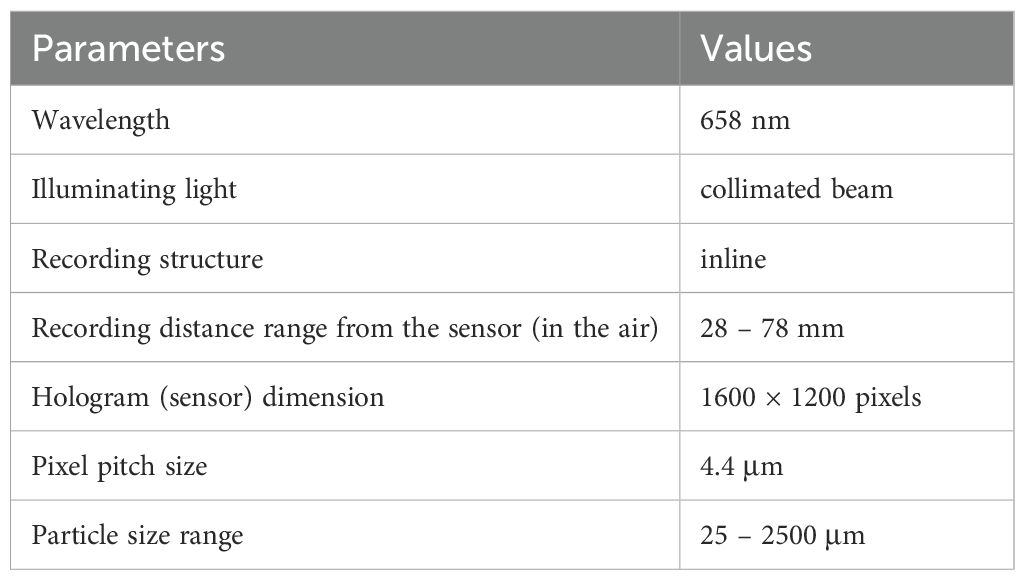
Table 1. Optical and configuration parameters of LISST-HOLO.

To visualize the recorded particles in digital holograms, holograms need to be first reconstructed numerically using a reconstruction algorithm on a computer. Additionally, a focus measure (Liu et al., 2023a) is needed to detect focused images of recorded particles. For this task, we used the particle image extraction suite, FastScan (Thevar et al., 2023), which can rapidly reconstruct and auto-focus inline digital holograms recorded using collimated laser beams, and output the vignettes of imaged particles. FastScan uses the Angular Spectrum algorithm to reconstruct holograms (Liu et al., 2023a; Schnars et al., 2015), and a contour-gradient-based auto-focus algorithm to extract recorded particles from the reconstructed holograms (Burns and Watson, 2014). These algorithms are implemented using parallel computation on a powerful Field Programmable Gate Array resulting in high processing speeds [838 Mp/s (Thevar et al., 2023)].

A total of 20,328 particle vignettes were extracted from the dataset. These vignettes were classified and manually verified using Ecotaxa². Noise/background particle vignettes were removed, and the remaining vignettes were sorted into 40 taxonomic classes. The 20 most representative classes (in terms of abundance and morphological diversity) were selected, yielding 8,902 vignettes. Examples of the extracted particle vignettes are shown in Figure 1.

Figure 1

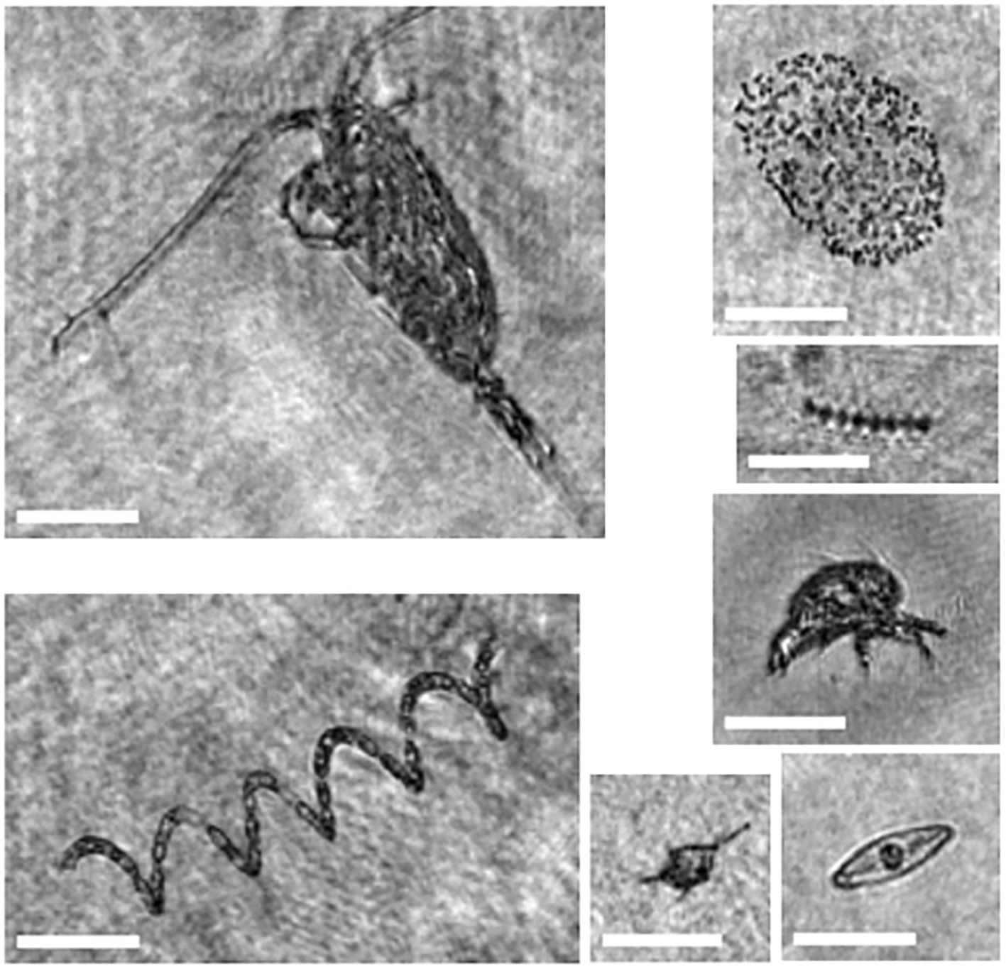
Figure 1. Sample particle vignettes extracted by FastScan in the dataset of natural particles recorded in situ. Each white bar indicates 100 μm.

2.2 Synthetic data simulation and processing

A synthetic holographic dataset, including reconstructed particle vignettes and their ground-truth edge images, was created (Figure 2). Each synthetic hologram was simulated based on the parameters of LISST-HOLO (Table 1). To simulate holograms, we used images of natural marine particles (zooplankton) imaged using ZooScan (Giering et al., 2019) due to their noiseless background and similar shape, complexity and resolution to objects imaged by LISST-HOLO. 877 ZooScan vignettes were binarized and used as the target pool. To simulate a synthetic hologram, up to 10 particles (vignettes) were randomly selected from the pool and randomly placed within the system’s recording optical path (28 to 78 mm depth from the camera sensor in the air). Each vignette was positioned at least 50 pixels away from each edge of the hologram. Details of each vignette in its synthetic hologram (location, size, and recording distance from the sensor) were stored. The dimension of each full-size synthetic hologram was the same as the holograms recorded by LISST-HOLO (1600 × 1200 pixels). Holograms were simulated using the Angular Spectrum method (Liu et al., 2023a; Schnars et al., 2015). Noise was added to the simulated holograms by taking real holograms without any targets and superimposing them as background noise in the simulated holograms. Specifically, the background hologram was first normalized with the maximum pixel value equal to the mean intensity of the simulated hologram (Liu et al., 2023a; Schnars et al., 2015); two holograms were then added together; and the intensity of the final hologram was lastly normalized into 0 – 255. The ‘recorded’ particles can be reconstructed from these simulated holograms based on the stored simulation information, and the ‘true’ edges can be extracted from the corresponding binarized ZooScan images.

Figure 2

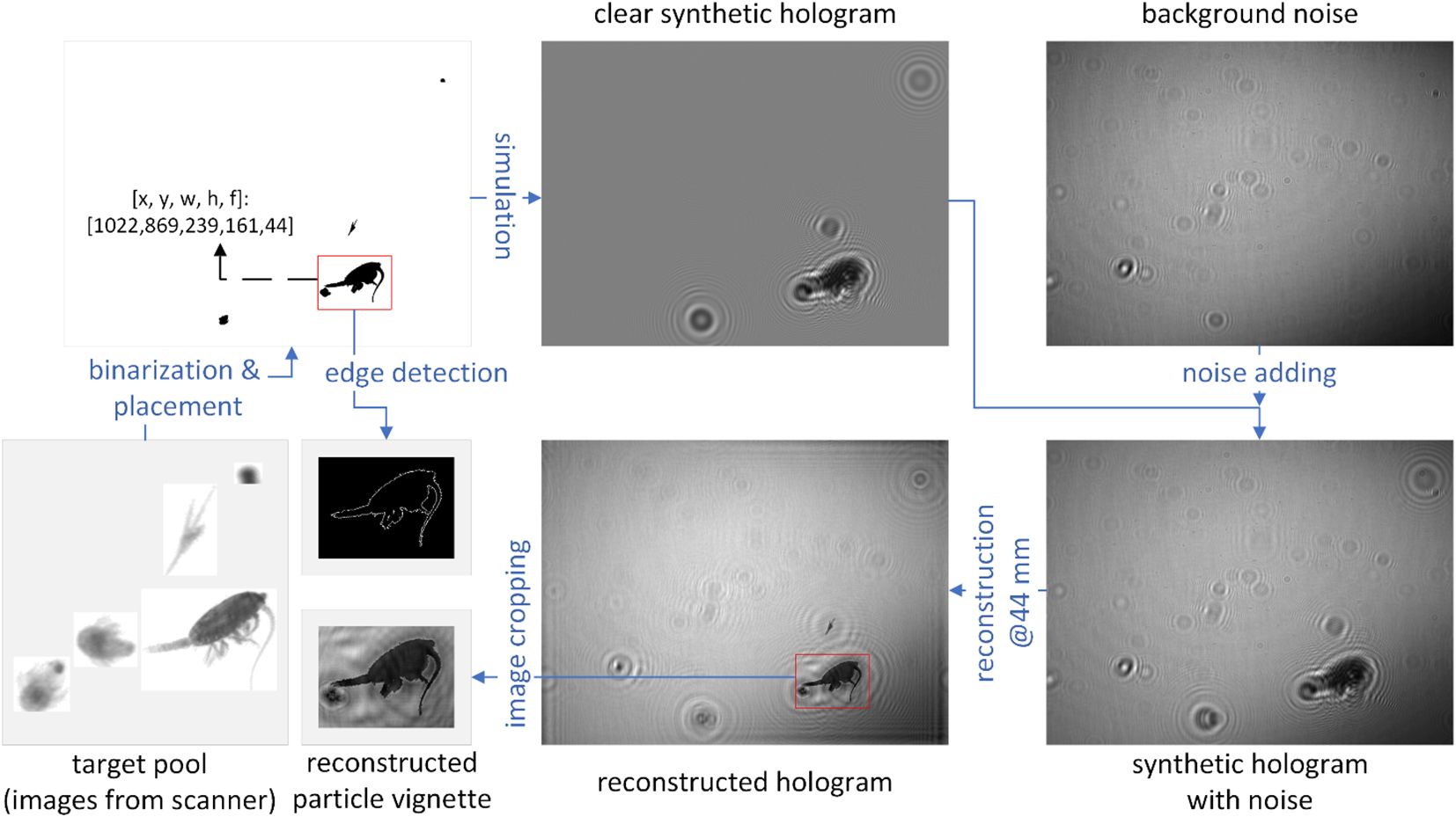
Figure 2. Workflow of data simulation. [x, y, w, h, f] indicates the details of the vignette in the synthetic hologram, including the top-left location in the hologram [x, y], vignette size [w, h], and recording distance from the sensor [f]. Each image size is adjusted for layout.

3 Methods

3.1 Methodology in HoloSForests

Our pipeline - HoloSForests, consists of three steps for estimating particles’ sizes (Figure 3). (1) An edge-detection model (structured forests) was trained twice using two different datasets: the model was first trained using the synthetic training dataset, and then fine-tuned using a small number of real, pixel-wise annotated holographic data from the natural oceanic dataset. (2) The trained model was used to extract particles’ edges in real holograms, and a set of morphological operations were then carried out in the extracted edge images to obtain their region masks. (3) Lastly, particles’ size information was estimated based on the calculated convex-hull region masks from the extracted region masks.

Figure 3

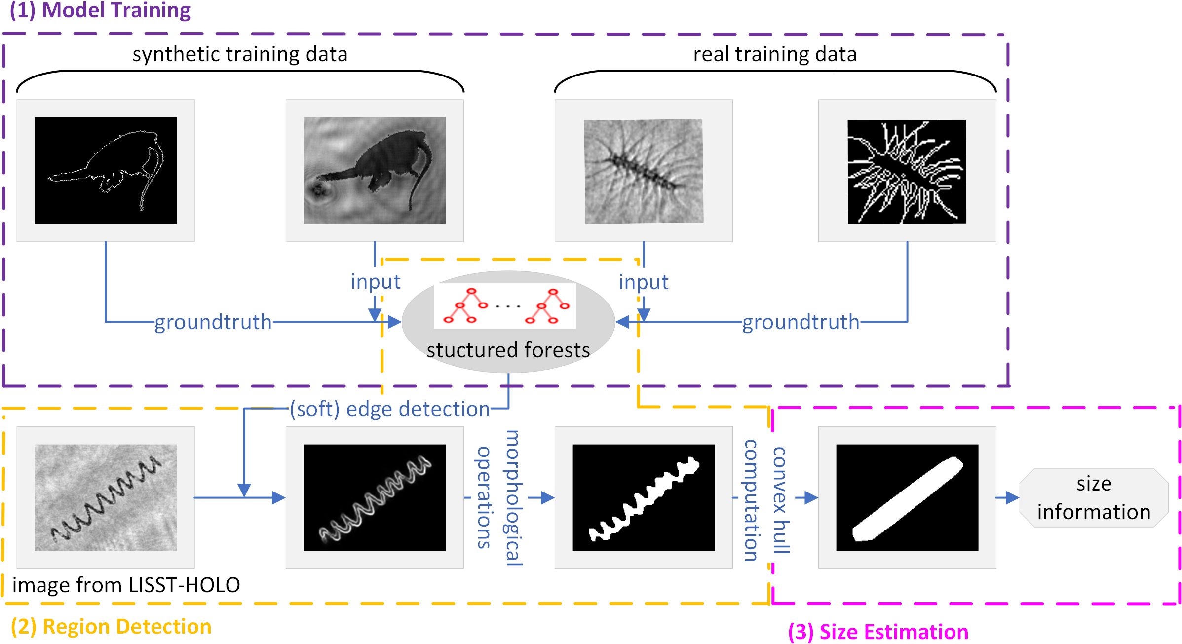
Figure 3. Workflow of HoloSForests to estimate the size information of particles in the particle vignettes. Three steps are contained in this workflow: (1) model training in the purple box, (2) edge-based region detection in the orange box, and (3) size estimation in the magenta box.

All the algorithms in HoloSForests were conducted on MATLAB (licence: 980953), and then ran on a computer with a processor of 12^th Gen Intel(R) Core(TM) i7-12700 and RAM of 16 GB.

3.1.1 Model training

We used the structured-forests-based model (referred to as structuredForests) by Dollár and Zitnick (2015) for the edge detection. The model consists of eight decision trees. In each tree, the maximum depth is 64, and the number of each of the positive and negative patches is 5 × 10⁵. To increase the diversity of the trees and edge-detection accuracy, the trees are trained independently, and the features and splits are randomly subsampled when training each node in each tree. Structured learning was used to map the edges between the input and output images in each tree. The eight trees are combined as a random forest to achieve robust outputs, and the overlapping edge maps are averaged to obtain a soft edge response. The ensemble model predicts a structured 16 × 16 segmentation mask (output) from a larger 32 × 32 image patch (input), thus with 16 × 16 output patches, each pixel receives 256 predictions. The score of each pixel in the output edge map is averaged over these 256 votes. A descriptive structure graph of the model is shown in Supplementary Figure 1 in Supplementary Material. The model codes are available from GitHub³.

The original weights of the model from the training on the Berkeley Segmentation Data Set 500 (BSDS, 500 natural images with annotated boundaries) (Martin et al., 2001) were used, since they provided good generalization on detecting the edges in natural images. The model (with original weights) was trained on our synthetic training data. To improve its performance on real holographic data, the trained model was further fine-tuned on our real holographic data based on the technique of transfer learning (Hosna et al., 2022; Pan and Yang, 2010).

3.1.2 Region extraction

structuredForests produces soft edge images, where each pixel value ranges from 0 to 1. In these images, higher pixel values indicate a higher probability of the pixel being located at an edge (second image of the bottom row in Figure 3). Therefore, the output edge images require further processing to extract particle size information.

A series of pixel-wise morphological operators were used on the output edge images (Figure 4). Since each edge image has high contrast between the particle edges and the background (second image of the bottom row in Figure 3), the thresholding algorithm Otsu [a fast binarization method based on the intra-class variance between the foreground and background (Otsu, 1979)] was used to determine the edge pixels in each edge image. The detected edges by the structured forest model are wide (Figure 3), resulting in an estimated particle area that is slightly bigger than the original. Therefore, if there were more than three pixels in the width direction of the edges, the edges in a binary edge image were thinned by removing one pixel from their two sides, respectively. To obtain the particle mask, the operation of hole filling was then used to fill the holes surrounded by edges in the binarized edge image. Subsequently, two steps were implemented to remove regions that were too small: morphological opening using a disk-shaped structure element with a diameter of 6 pixels and removing the regions that are smaller than 25 pixels. In the last step, regions within a 6-pixel distance from each other were merged in the mask image. The criteria of 6 and 25 pixels was chosen based on the minimum concentrated particle size (25 µm) and pixel size (4.4 µm) of LISST-Holo, as: $\frac{25 \mu \text{m}}{4.4 \mu \text{m}}\approx 6$ and $\frac{\pi {(\frac{25 \mu \text{m}}{2})}^2}{{(4.4 \mu \text{m})}^2}\approx 25$.

Figure 4

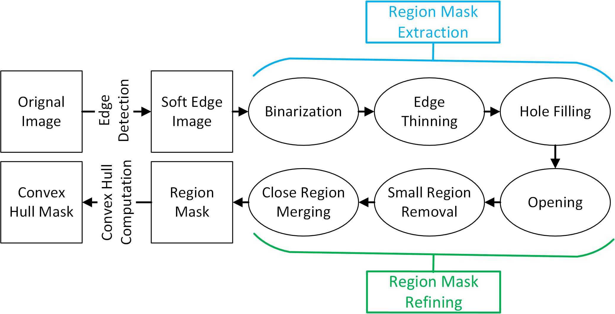
Figure 4. Flow chart of pixel-wise morphological operations for extracting the region masks from the edge image output from structuredForests.

3.1.3 Particle size estimation

Since hole filling is applied in the workflow, an extracted region by the proposed method might not be the actual region for a particle, particularly when a string-shape particle forms a circular pattern in the image. Therefore, the size information of particles obtained using the proposed method is expected to have less bias to such particles, if it is calculated in terms of the convex hull region.

Three concepts were used to describe particle size based on the extracted convex hull region: (1) major-axis length (the Euclidean distance of the two furthest points in a region boundary), (2) minor-axis length (the Euclidean distance of the two closest points in a region boundary), and (3) equivalent spherical diameter (ESD) (Giering et al., 2020b). ESD describes the size of an irregularly shaped object using the diameter of a sphere which has the same area as the object. It is calculated as Equation 1:

$\begin{array}{ll}\text{ESD}=2\sqrt{\frac{A_{conhull}}{\pi }}& (1)\end{array}$

where $A_{conhull}$ is the convex hull area of a particle which is calculated as $A_{conhull}=\sum i,j{R}_{conhull}(i,j)\times {(4.4 \text{μm})}^2$ with $R_{conhull}$ indicating a binary convex hull mask of the particle, and 4.4 µm indicating the pixel pitch size of LISST-HOLO. Since LISST-HOLO can only detect particles whose ESDs are in the range from 25 to 2500 µm, those particles whose ESDs are not in this range are omitted when estimating particle size.

Note that hull-based size estimates are higher compared to the pixel-based size estimates for natural particles with highly irregular, concave or porous shapes. Yet, this metric is useful as an upper bound for drag estimation, assessing particle morphology [e.g., ‘solidity’ and ‘roundness’ (Giering et al., 2020b)], and the space taken up by particles.

3.2 Datasets for model training and evaluation

A total of three datasets were created for model training and evaluation: a synthetic holographic dataset and two real holographic datasets. One real holographic dataset of standardized basalt spheres for model evaluation is described in Section 5 of Supplementary Material.

3.2.1 Synthetic holographic data (SHD)

One thousand synthetic holograms containing a total of 7,000 marine particles were created using the method described in Section 2.2. Each simulated hologram was reconstructed at the z-distances where the ZooScan vignettes had been placed, and the reconstructed particles were extracted and saved. 3,000 of the 7,000 reconstructed particle images were randomly selected to create the training dataset. These reconstructed images and the edge images from their original vignettes were used, respectively, as the input and ground-truth images for training the model (Figure 2). We chose this number because the performance of trained models on edge detection did not obviously change when more than 3,000 particles were used (Section 2 in Supplementary Material). An additional 1,000 pairs of reconstructed particle images and original edge images were randomly selected from the rest of the synthetic dataset as the testing data. This SHD dataset was used to test the edge detection performance of structuredForests, as well as the region extraction performance of HoloSForests.

3.2.2 Real holographic data - cruise (RHD-Cruise)

We compiled a training/testing dataset with natural and complex marine particles. For this, we selected 5 representative particle vignettes from each of the 20 taxonomic classes (Table 2), yielding a dataset with 100 particle vignettes (Supplementary Figure 3 in Supplementary Material). Three people manually labelled the particle regions pixel by pixel in each vignette, and a pixel was designated as a part of the region if at least two people labelled it as a region pixel. The edges of the particle(s) in each region mask (Table 2) are detected used the method proposed by Liu et al. (2018). This dataset was used for two parts of work: (1) when evaluating HoloSForests’ performance across the entire data, 3 particle vignettes from each class were randomly selected for training, and the remaining 2 vignettes were used for testing (i.e., 60 real holographic vignettes as the training data and 40 vignettes as the test data); (2) when evaluating the capability of HoloSForests for estimating the size of particles for different taxonomic classes, 5-fold cross validation (King et al., 2021) was adopted. For this, 1 vignette in each class was used as test data, and the remaining 4 vignettes were used as train data, and the process was iterated until every vignette in each class was used as test data.

Table 2

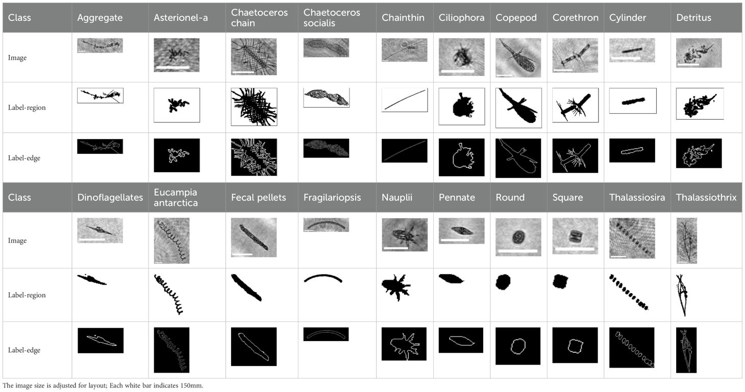
Table 2. One example for each taxonomic class, and its labelled particle region and edges.

3.3 Evaluation metrics

Two metrics were adopted to evaluate the accuracy performance of HoloSForests in terms of edge detection and region extraction. Furthermore, the time efficiency (i.e., running time) was also evaluated.

3.3.1 Structural similarity index measure (SSIM)

SSIM (Wang et al., 2004) was selected to evaluate the accuracy performance of edge detection. It measures the similarity between two images based on three features: luminance, contrast, and structure. As a result, it provides a better evaluation of image similarity compared to measures that rely solely on the intensity of corresponding pixels in the two images. SSIM = 1 indicates that the two images are the same; the smaller the value is, the more different the two images are. SSIM is calculated as Equation 2:

$\begin{array}{ll}\text{SSIM}(r,gt)=\frac{(2{\mu }_r{\mu }_{gt}+C_1)(2{\sigma }_{r,gt}+C_2)}{({\mu }_r^2+{\mu }_{gt}^2+C_1)({\sigma }_r^2+{\sigma }_{gt}^2+C_2)}& (2)\end{array}$

where $\mu$ and $\sigma$ indicate the mean value and standard deviation of an image, ${\sigma }_{r,gt}$ is the covariance of two images; $C_1$ and $C_2$ are two small constants to stabilise the division with a weak denominator that are calculated by $C_1={(K_{1}L)}^2$ and $C_2={(K_{2}L)}^2$ where $K_1=0.01$, $K_2=0.03$, and $L=255$ for 8 bits/pixel images.

3.3.2 Intersection over union (IoU)

The accuracy of region extraction was evaluated using IoU (Rezatofighi et al., 2019). It is a key metric to measure the accuracy of region extraction based on binary images and is computed as the ratio of the overlap of the predicted region ($r$) and ground truth $gt$) as Equation 3:

$\begin{array}{ll}\text{IoU}(r,gt)=\frac{\text{TP}}{\text{TP}+\text{FP}+\text{FN}}& (3)\end{array}$

where $\text{TP}$ is the intersected area between $r$ and $gt$ ($\text{TP}=r\cap gt$), $\text{FP}$ is the area that is predicted to be part of the region but is not actually part of the ground truth ($\text{FP}=r\cup gt-gt)$, and $\text{FN}$ is the area that is part of the ground truth but is not predicted as part of the region ($\text{FN}=r\cup gt-r$). A perfect overlap of the predicted region and ground truth region has an IoU value of 1 ($r=gt)$.

3.4 Evaluation and validation

3.4.1 Optimization of edge detection capabilities of structuredForests using synthetic data

Since the original structuredForests trained on the BSDS data demonstrates good generalization in the original work, we investigated how different training strategies performed in detecting particle edges in holographic images. For this, five models were generated by training on five different dataset combinations: Model 1 was trained on BSDS (n = 500), Model 2 was trained on BSDS and RHD-Cruise (n = 500 + 60, respectively), Model 3 was trained on BSDS and SHD60 (n = 500 + 60, respectively; with 60 training images randomly selected from the 3,000 training images in SHD), Model 4 was trained on BSDS and SHD (n = 500 + 3,000, respectively), and Model 5 was trained on BSDS, SHD and RHD-Cruise (n = 500 + 3000 + 60, respectively). The five models were then used to predict particle edges in the test images from the SHD and RHD-Cruise datasets (1,000 and 40 test images, respectively). Since the models produce the soft edges for an input image, SSIM-related measures - including its mean (mSSIM, reflecting the overall accuracy) and standard deviation (stdSSIM, reflecting the robustness) - were used to evaluate the five models.

3.4.2 Comparison of HoloSForests with other region extraction methods

HoloSForests was compared with ten other methods (Liu et al., 2023b), including four edge-based methods (cannyEdge, sobelEdge, prewittEdge, and robertsEdge), four region-based methods (activeContour, regionGrowing, SRegionMerging, and Watershed), a thresholding-based method (OtsuThresholding), and a clustering-based method (KMeans). In the four edge-based methods, the same morphological operations (excluding binarization and edge thinning) were used to extract the region masks from their output edge images. In the other six methods, the operations for Region Mask Refining (Figure 4) were used to refine the extracted region masks. Additionally, we evaluated the capability of HoloSForests in region extraction for particles from different taxonomic classes (20 classes in RHD-Cruise) using the 5-fold cross validation (Section 3.2). Since extracted region masks are binary, IoU-related measures - including its mean (mIoU, reflecting the overall accuracy) and standard deviation (stdIoU, reflecting the robustness) - were used to evaluate these eleven methods.

3.4.3 Real-word application

HoloSForests was used to analyze the vertical distribution of particle size in two depth profiles (Event 034 and Event 098) recorded during the ocean research expedition. Due to the high noise levels in particle images from the surface to 4 m depth (Giering et al., 2020b), the size distribution was assessed below this depth.

4 Results and discussion

Here we present and evaluate the performance of HoloSForests in terms of edge detection, region extraction, and size estimation.

4.1 Optimization of edge detection capabilities of structuredForests using synthetic data

First, we assessed the effectiveness of structuredForests in detecting particle edges in reconstructed holograms, using both synthetic and real datasets (Table 3). As expected, even though the original model shows good generalisation (Model 1), training on holographic images (Model 2-5) improves both metrics (mSSIM and stdSSIM): Model 1 is least accurate (smallest mSSIM) and least robust (largest stdSSIM) on both test datasets. Therefore, the model should be trained on holographic data to detect particle edges in holographic images. The results of Model 2 and Model 3 shows that training with few holographic images (n = 60) improves the model performance in accuracy and robustness, however, the output is domain-specific, particularly regarding accuracy: training on synthetic data improves performance on both synthetic and real data, but more on synthetic, while training on real data enhances both, with greater gains on real data. This domain specificity becomes weak when the model is trained on a large synthetic dataset (n = 3,000): compared to Model 1, increasing of mSSIM in Model 4 by 25.0% on the synthetic data and 23.7% on the real data, respectively. Although our most comprehensively trained model (Model 5, trained on both real and synthetic data) performs similarly on the synthetic test data compared to Model 4, its performance is slightly better on the real test data. We conclude that training on synthetic data is an effective way to improve edge detection in holographic images; the addition of even a small number of real images (2%) improves the model’s edge detection accuracy and robustness on real holographic data.

Table 3

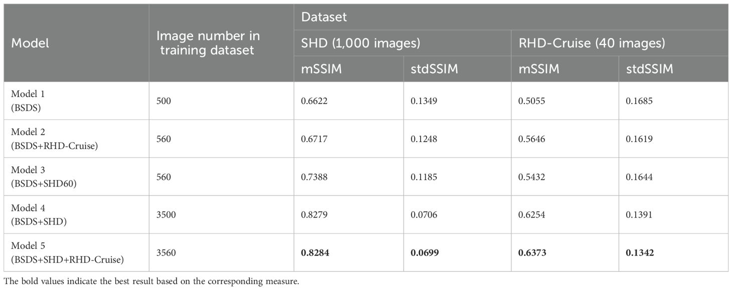
Table 3. Performance evaluation of structuredForests on edge detection on the synthetic and real holographic datasets in terms of accuracy (mSSIM and stdSSIM) after it is trained on the five different datasets.

The results from the performance evaluation (Table 3) are supported by visual inspection of the predicted edges of three example images from both the synthetic and real holographic datasets (Figure 5). For both synthetic and real holographic example images, we can see that the edge images output from the extensively trained models (Models 4 and 5) have clean backgrounds and clear edges (the pixel values along edges are higher), while the corresponding images from the base model (Model 1) and low-level trained models (Models 2 and 3) show more fake edges (noise) around the particles or across the entire image. This visual inspection also demonstrates that the predicted edges are wider than the labelled edges in ground truth images, likely as a result of the soft detection scheme in the models. This widening could cause a slight overestimate on a particle’s area compared to its actual area. For this reason, we employed the operation of edge thinning as a part of the morphological operations (Figure 4).

Figure 5

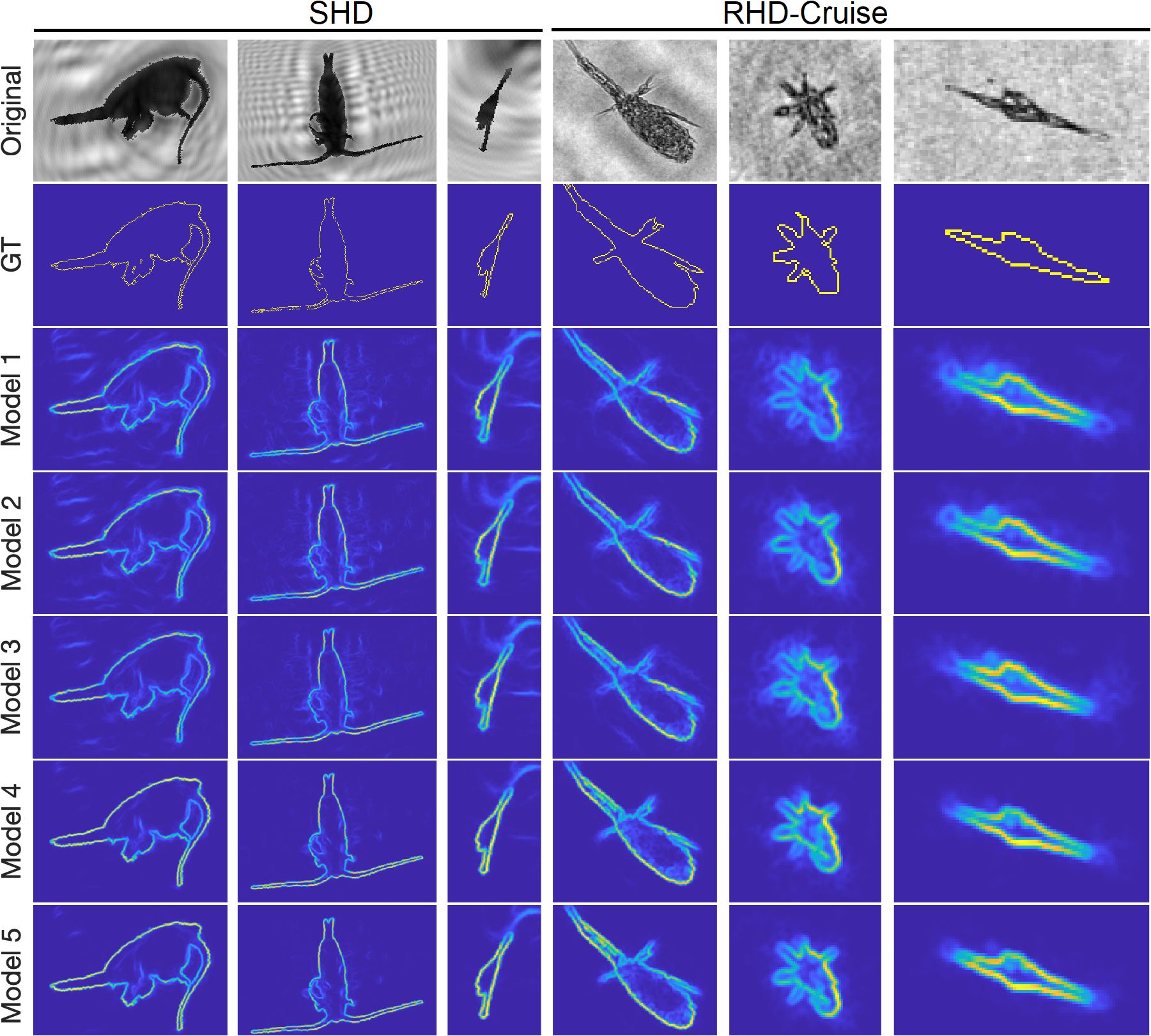
Figure 5. Edge images of the synthetic and real holographic image examples output from the five models described above. GT – ground-truth images. The pixel value scale is converted into [0, 255] from [0, 1] in the edge images for displaying them.

Overall, our Model 5, which is trained on both the synthetic and real holographic datasets, performs best in terms of accuracy and robustness. We therefore used this model to detect particle edges in the rest of our experiments (unless stated otherwise).

4.2 Comparison with other region extraction methods

4.2.1 Performance on entire data

The proposed series of pixel-wise morphological operations by HoloSForests (Figure 4) for extracting the region mask and the convex hull from the reconstructed images are effective in defining the area of even complex particles, like large colonial diatoms whose ‘inner texture’ is similar to the background noise (Figure 6).

Figure 6

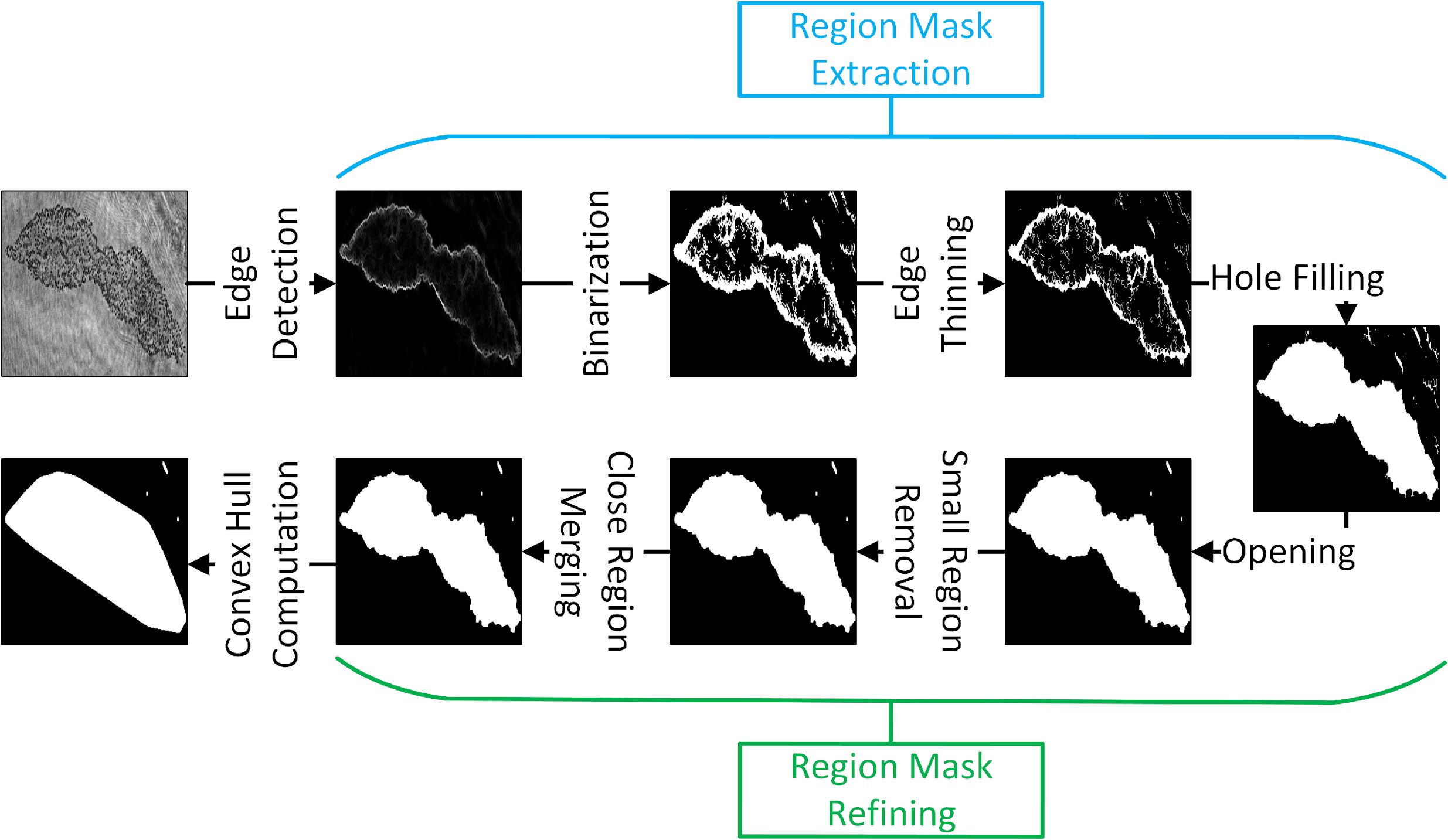
Figure 6. Resultant output of each step in HoloSForests when processing one image example. The image size is adjusted for layout.

Regarding accuracy and robustness, HoloSForests outperforms the ten other region extraction algorithms (Table 4). On the synthetic data, it markedly outperforms the other 4 edge-based methods in terms of accuracy (mIoU: 0.81 vs 0.38 – 0.58, respectively) and robustness (stdIoU: 0.18 vs 0.19 – 0.38, respectively). SRegionMerging is the best region-based method, yet it is slightly less accurate (mIoU: 0.79) than HoloSForests. Moreover, its robustness is lower compared with HoloSForests (stIoU: 0.23 vs 0.18, respectively). Similarly, the accuracy of KMeans (mIoU: 0.78) is close to the one of HoloSForests, but it is less robust (stdIoU: 0.20). OtsuThresholding is the fourth best method with mIoU of 0.71. Another region-based method - regionGrowing, is the least accurate method (mIoU: 0.32) amongst all the 11 methods.

Table 4

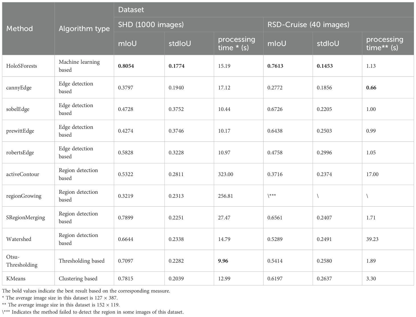
Table 4. Performance of the methods on region extraction on the synthetic and real holographic datasets in terms of the efficiency of accuracy (mIoU and stdIoU) and time.

On the real holographic data, the accuracy of 9 of the 11 algorithms decreases relative to their performance on the synthetic data (Table 4). regionGrowing even fails to detect the regions in some images. Surprisingly, sobelEdge and prewittEdge are more accurate and robust on the real data than on the synthetic data, improving accuracy by ~0.20 and robustness by ~0.12. HoloSForests remains the best method with only slight changes in accuracy (a decrease of 0.04) and robustness (a decrease of 0.03), which shows good generalization for both synthetic and real holographic images. SRegionMerging becomes the third most-accurate method (0.66), as sobelEdge takes the second place (0.67). Amongst the 5 methods with reasonable accuracy (mIoU > 0.6), KMeans performs the worst. With an accuracy of < 0.5, cannyEdge, robertsEdge, and activeContour are not suitable for detecting particle regions in the real holographic test data.

Regarding the processing time, with the exception of activeContour and regionGrowing, we are able to process the 1,000 synthetic holographic images within 30 seconds with all methods. In contrast, both activeContour and regionGrowing take more than 4 minutes. OtsuThresholding has the shortest processing time of ~10 seconds. Although HoloSForests takes ~15 seconds to process 1,000 images, this speed still enables it to instantly generate an output once it receives an input image [real-time processing (Dougherty and Laplante, 1995)]. To detect the regions in the 40 real holographic images, most methods take < 4 seconds, apart from activeContour (~17 seconds), Watershed (~39 seconds) and regionGrowing (stuck in detecting the regions in some images). Although cannyEdge is the fastest method (0.66 second), it has the lowest accuracy compared to the other algorithms (except for regionGrowing). While HoloSForests is not the fastest method, among those with reasonable accuracy (mIoU > 0.6), its processing speed is only marginally slower than the fastest algorithm (1.13 seconds vs. 0.99 seconds) and remains acceptable for real-time data processing.

To visualize the performance of the 11 algorithms, we showed the extracted regions for example holographic images from five of the complex plankton classes (Figure 7). Qualitatively analysed, the performance rank of the methods is similar with the calculated performance metrics (Table 4). HoloSForests performs consistently well on the five images, with fine features at a reasonable level, such as the complex shape of colony-forming diatoms and the appendages of zooplankton. Other methods that also perform reasonably well are sobelEdge, prewittEdge, and SRegionMerging. In contrast, cannyEdge, activeContour, and regionGrowing cannot detect the plankton in any of the images, likely because of the high background noise from interference patterns in the reconstructed holograms. robertsEdge, Watershed, OtsuThresholding, and KMeans can detect the plankton in some images, however, they also introduce false regions and/or miss real ones, likely due to the noisy background.

Figure 7

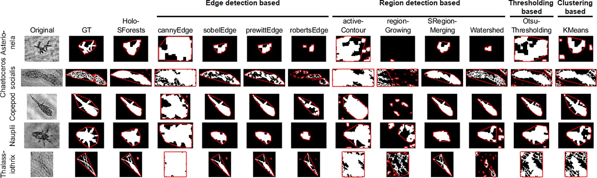
Figure 7. Regions (in white) and boundaries of their convex hulls (in red) extracted from five examples of the real holographic test data. The images have been resized for the layout purpose.

4.2.2 Performance on individual taxonomic classes

As the complexity of a particle’s shape influences the ability of an algorithm to correctly identify the particle regions, we here investigated how size estimation varies for different plankton classes. To do so, we compared HoloSForests to the other top 4 algorithms (sobelEdge, SRegionMerging, prewittEdge, KMeans; Table 4) in terms of mIoU on the RSD-Cruise test data. HoloSForests overperforms the other 4 methods in all classes apart from the class of chain-forming diatom Thalassiosira (Figure 8S), where sobelEdge and prewittEdge are more accurate (mIoU: 0.64 vs 0.71 and 0.68, respectively; Supplementary Table 1 in Supplementary Material). It clearly outperforms the other methods for classes with fine features, such as appendages and spikes (e.g., Chaetoceros sp., copepods and nauplii; Figures 8C, G, O) and complex shapes (e.g., aggregates and Asterionella sp.; Figures 8A, B). HoloSForests was least accurate for thin and long particles (class Chainthin; mIoU = 0.58). The discrepancies may be due to the relatively wide edges that it predicts and which require thinning. For long objects that are only a few pixels wide, a small change in width will lead to big differences in relative size estimates. However, even for this class, HoloSForests still performs remarkably better than the other 4 methods (mIoU: 0.11 – 0.37; Supplementary Table 1 in Supplementary Material).

Figure 8

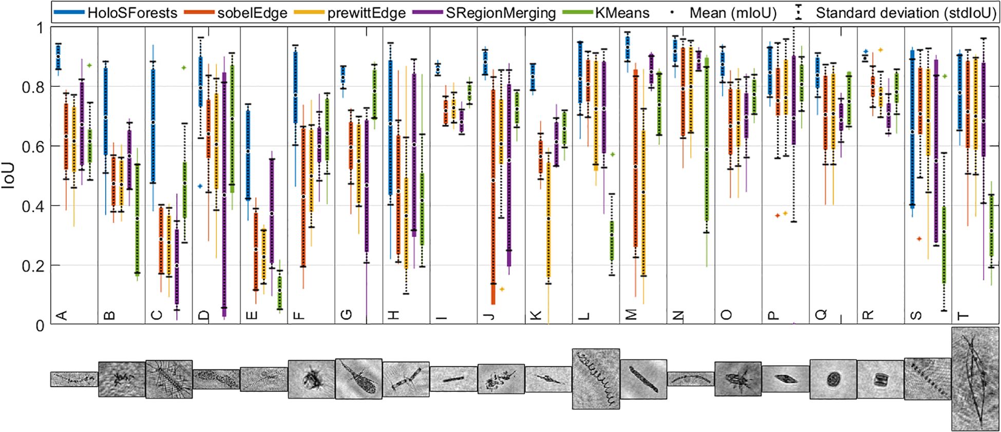
Figure 8. Box plotting of the results of 5 methods when evaluating them on the images of each class of 20 classes. (A) Aggregate, (B) Asterionella, (C) Chaetoceros chain, (D) Chaetoceros socialis, (E) Chainthin, (F) Ciliophora, (G) Copepod, (H) Corethron, (I) Cylinder, (J) Detritus, (K) Dinoflagellates, (L) Eucampia antarctica, (M) Fecal pellets, (N) Fragilariopsis, (O) Nauplii, (P) Pennate, (Q) Round, (R) Square, (S) Thalassiosira, (T) Thalassiothrix. The example of each class shown in Table 2 is given for visualization of them.

Another advantage of HoloSForests is its robust performance across most classes (as determined by stdIoU in Supplementary Table 1 in Supplementary Material, and visualized by the short boxes in Figure 8). HoloSForests deviates by ≤ 0.05 mIoU for 8 of the 20 classes (Square, Cylinder, Copepod, Detritus, Aggregate, Dinoflagellates, Fecal pellets, and Fragilariopsis). In contrast, the second-best method - SRegionMerging - performs similarly well for only 3 classes; while the remaining 3 methods can achieve this robustness for only 1 class each. The most robust performance of HoloForests comes from the class Square (stdIoU = 0.01; Supplementary Table 1 in Supplementary Material), which contains simple square-like particles (such as the side view of centric diatoms). Interestingly, the value for another simple shape - Round (stdIoU = 0.07; Supplementary Table 1 in Supplementary Material) is higher than for some of the more complicated shapes (e.g., Aggregates). Possible explanations could be: (1) the regions of round particles are generally very small such that a small difference between the extracted region and ground-truth regions can cause a big decrease in IoU; (2) regular holographic fringes (i.e., noise) usually occur around reconstructed round particles, which cause instability in extracting their regions. The least robust classes are Corethron sp., Thalassiosira sp., and chain-forming Chaetoceros sp. (stdIoU = 0.27, 0.24, and 0.20, respectively; Supplementary Table 1 in Supplementary Material), since these particles have many fine structures and/or multiple disconnected components (Table 2).

Overall, HoloSForests has good accuracy and robustness when extracting the regions of complex natural particles from reconstructed holograms.

4.3 Real-world application

Histogram analysis (Figures 9-1, 2) indicates the expected long-tailed distribution: the majority of detected particles (> 90%) had hull-based ESDs smaller than 500 μm, while only a small fraction (< 1%) exceeds 1000 μm. The scarcity of large particles is likely due to a low abundance of particles of this size within the sampling area, though we cannot completely rule out limitations in the FastScan reconstruction algorithm for very large particles. However, given that some particles exceeding 1000 μm were successfully reconstructed by FastScan (Supplementary Figure 5 in Supplementary Material), it is likely that the low detection rate of these larger particles reflects their true low abundance in the observation area at the time of data collection.

Figure 9

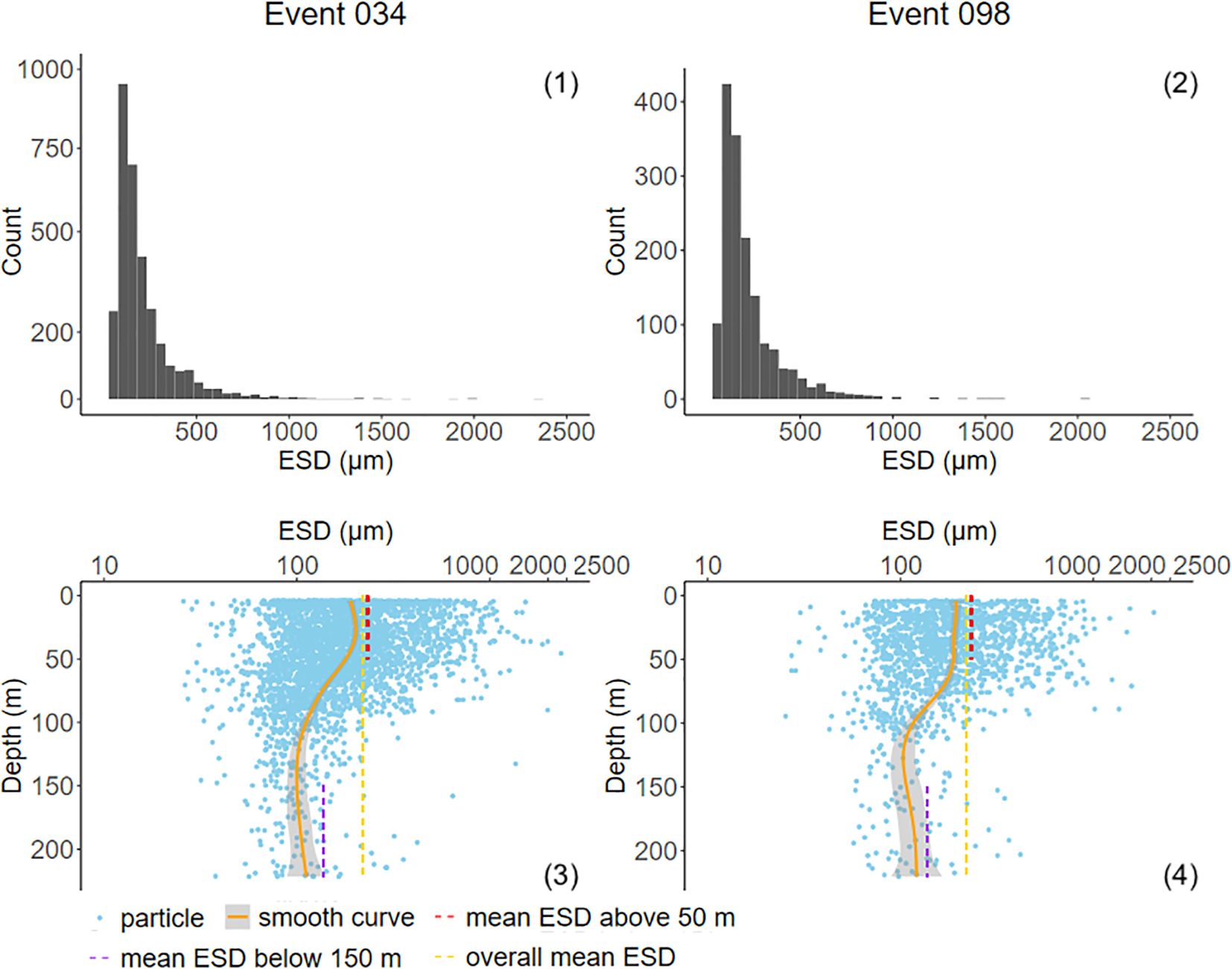
Figure 9. (1-2) Histograms showing particle size in 50 bins for the two profiles (1: Event 034, and 2: Event 098). (3-4) Vertical profiles of particle size (hull-based ESD) estimated using HoloSForests from two deployments (3: Event 034, and 4: Event 098). The solid orange lines follow the smoothed average. The dashed lines show the mean hull-based ESD in the depth ranges 4 – 50 m (red), 150 – 230 m (purple), and 4 – 230 m (orange). Please note that the x-axis is logarithmic in the bottom two graphs.

Both profiles (Figures 9-3, 4) exhibit similar trends in particle size distribution, with a general decrease in particle size with increasing depth. Notably, the mean hull-based ESD (Table 5) shows a marked reduction between 50 m and 150 m depth. The mean ESD decreased from 245.5 ± 202.9 μm to 123.0 ± 87.4 μm from above 50 m to below 150 m in Event 034; while in Event 098, it declined from 232.6 ± 179.0 μm to 136.5 ± 83.1 μm (above 50 m and below 150 m, respectively). The average particle size across the entire water column was 211.8 ± 182.6 μm and 218.2 ± 177.4 μm in Event 034 and Event 098, respectively.

Table 5

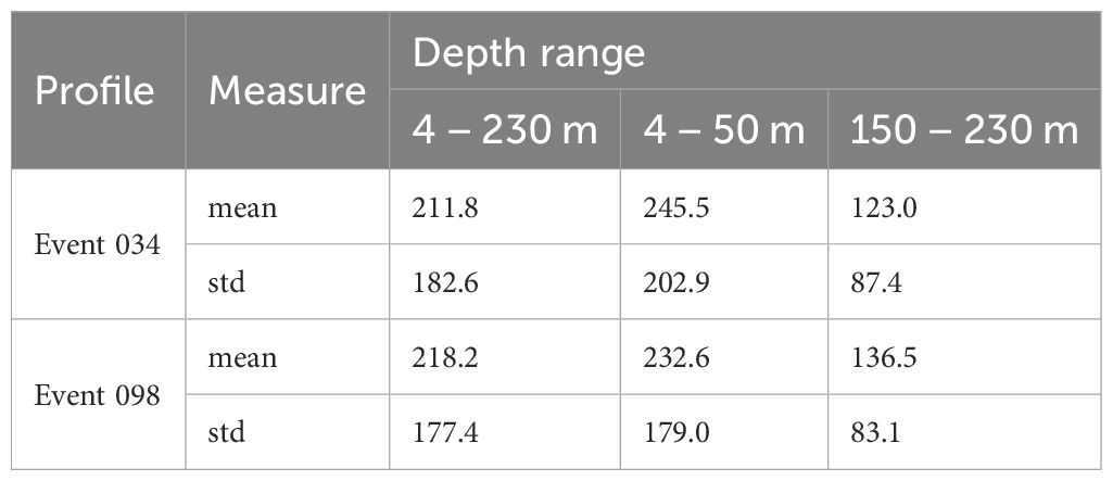
Table 5. Mean values (mean) and stand deviation values (std) of the two profiles in different depth ranges.

These size estimates are slightly smaller than previous estimates of these particle profiles based on reconstructed images made using the software HoloBatch combined with a sequence of image processing steps aimed to avoid fragmentation of complex particles (Planktonator; Giering et al., 2020b). The final vignettes in that workflow had a clear white background, and particle regions were hence determined using a range of region detection methods, with Otsu being used as the reference algorithm. As the original work used pixel-wise ESD, we recalculated their size estimates using hull-based ESD and calculated mean sizes across the entire water column. The recalculated values (234 ± 225 μm and 246 ± 239 μm for Event 034 and Event 098, respectively) are ~10% higher than the size estimates by HoloSForests. Compared to the previous work (Giering et al., 2020b), our workflow here has several advantages. Besides the faster hologram reconstruction time (using FastScan compared to HoloBatch), visual inspection shows that FastScan is less prone to fragment large complex plankton (such as Chaetoceros socialis) than HoloBatch. The higher size estimates observed with HoloBatch + Planktonator are likely due to Planktonator’s tendency to over-combine particles, potentially incorporating ‘false’ particles created by interference patterns, when particle abundance is high.

Overall, HoloSForests applies less image manipulation, which likely provides images closer to reality (albeit with noisy background). Lastly, we validated size estimates by HoloSForests using both human pixel-wise annotations and size-sorted basalt spheres (Section 5 in Supplementary Material), providing an evidence base for the accuracy of the produced size estimates.

5 Conclusions

Images provide valuable information on marine particle size. DIH, with its high resolution and capacity for relatively large-volume recording, is a powerful tool for imaging marine microscale particles. However, extracting particle size from holograms remains challenging owing to the complex shape of naturally occurring particles and background noise in reconstructed holograms. This paper presents a method developed to address these challengers, which involves two primary steps: (1) training a structured forest model on three datasets – BSDS500, synthetic holographic data, and real holographic data - to detect the particle edges in images; and (2) applying a series of pixel-wise morphology operators (including binarization, edge thinning, hole filling, morphological opening, small-region removal, close-region merging, convex hull) on the edge-detection outputs to extract the particle regions and convex-hull masks. Particle size information is subsequently estimated from the extracted regions.

Our five main findings are:

1. The training strategy on a combination of synthetic holographic images and a small number of real holographic images increases the accuracy of particle region extraction in holograms.

2. Amongst the 11 region detection methods tested in this work, the proposed method HoloSForests gives the highest accuracy when extracting particle regions from the synthetic and real test images (respective mIoU of ~0.81 and ~0.76) at competitive processing speeds.

3. HoloSForests can accurately extract the regions of naturally occurring oceanic particles with complicated shapes, such as aggregate, Chaetoceros sp. chains, and chain-like thin particles.

4. HoloSForests has the capability of providing accurate size information of recorded particles in holograms, even when multiple particles with complicated shapes exist in the same image.

5. Synthetic holographic data is a useful alternative to human-annotated data for training a machine-learning-based model for object detection/segmentation in holograms, particularly when it is not practical to prepare a large amount of human-annotated data.

Overall, we propose that our method is capable of rapidly and accurately extracting particle regions from reconstructed holographic images, as well as estimating the particle size accurately.

Data availability statement

The datasets presented in this study can be found in online repositories. The names of the repository/repositories and accession number(s) can be found in the article/supplementary material.

Author contributions

ZL: Conceptualization, Data curation, Formal Analysis, Investigation, Methodology, Software, Validation, Visualization, Writing – original draft, Writing – review & editing. MT: Data curation, Writing – review & editing. YC: Data curation, Writing – review & editing. TT: Software, Writing – review & editing. AN-S: Data curation, Writing – review & editing. JW: Software, Writing – review & editing. SG: Data curation, Formal Analysis, Funding acquisition, Project administration, Resources, Supervision, Writing – review & editing.

Funding

The author(s) declare financial support was received for the research and/or publication of this article. Some data used in this work was collected as part of the COMICS project (Controls over Ocean Mesopelagic Interior Carbon Storage; NE/M020835/1) funded by the Natural Environment Research Council. This work was supported through the ANTICS project, receiving funding from the European Research Council (ERC) under the European Union’s Horizon 2020 research and innovation programme (Grant Agreement No 950212).

Acknowledgments

We thank Richard Lampitt, Morten Iversen and Kevin Saw for the deployment of the Red Camera Frame, and the captain, crew and scientists of the research cruise DY086. Our thanks extend to Nick Burns and Mike Ockwell from Hi-Z 3D LTD (London, UK) for their contributions in developing FastScan that significantly facilitates hologram process.

Conflict of interest

The authors declare that the research was conducted in the absence of any commercial or financial relationships that could be construed as a potential conflict of interest.

Generative AI statement

The author(s) declare that no Generative AI was used in the creation of this manuscript.

Publisher’s note

All claims expressed in this article are solely those of the authors and do not necessarily represent those of their affiliated organizations, or those of the publisher, the editors and the reviewers. Any product that may be evaluated in this article, or claim that may be made by its manufacturer, is not guaranteed or endorsed by the publisher.

Supplementary material

The Supplementary Material for this article can be found online at: https://www.frontiersin.org/articles/10.3389/fmars.2025.1587939/full#supplementary-material

Footnotes

1. ^ https://www.comm-tec.com/Docs/Manuali/Sequoia/LISST-HOLO-manual-v3.0.pdf.
2. ^ https://ecotaxa.obs-vlfr.fr/gui/index.
3. ^ https://github.com/pdollar/edges.

References

Nayak A. R., Malkiel E., McFarland M. N., Twardowski M. S., and Sullivan J. M. (2021). A review of holography in the aquatic sciences: in situ characterization of particles, plankton, and small scale biophysical interactions. Front. Mar. Sci. 7, 572147. doi: 10.3389/fmars.2020.572147

Crossref Full Text | Google Scholar

Burns N. and Watson J. (2014). Robust particle outline extraction and its application to digital in-line holograms of marine organisms. Opt. Eng. 53, 112212. doi: 10.1117/1.OE.53.11.112212

Crossref Full Text | Google Scholar

Dollár P. and Zitnick C. L. (2015). Fast edge detection using structured forests. IEEE Trans. Pattern Anal. Mach. Intell. 37, 1558–1570. doi: 10.1109/TPAMI.2014.2377715

PubMed Abstract | Crossref Full Text | Google Scholar

Dougherty E. and Laplante P. (1995). “What is real-time processing?,” in Introduction to real-time imaging (Wiley-IEEE, New York, US), 1–9.

Google Scholar

Giering S. L. C., Cavan E. L., Basedow S. L., Briggs N., Burd A. B., Darroch L. J., et al. (2020a). Sinking organic particles in the ocean—flux estimates from in situ optical devices. Front. Mar. Sci. 6, 834. doi: 10.3389/fmars.2019.00834

Crossref Full Text | Google Scholar

Giering S., Culverhouse P. F., Johns D. G., McQuatters-Gollop A., and Pitois S. G. (2022). Are plankton nets a thing of the past? An assessment of in situ imaging of zooplankton for large-scale ecosystem assessment and policy decision-making. Front. Mar. Sci. 9, 986206. doi: 10.3389/fmars.2022.986206

Crossref Full Text | Google Scholar

Giering S. L. C., Hosking B., Briggs N., and Iversen M. H. (2020b). The interpretation of particle size, shape, and carbon flux of marine particle images is strongly affected by the choice of particle detection algorithm. Front. Mar. Sci. 7, 564. doi: 10.3389/fmars.2020.00564

Crossref Full Text | Google Scholar

Giering S., Wells S. R., Mayers K. M. J., Schuster H., Cornwell L., Fileman E. S., et al. (2019). Seasonal variation of zooplankton community structure and trophic position in the Celtic Sea: A stable isotope and biovolume spectrum approach. Prog. Oceanogr. 177, 101943. doi: 10.1016/j.pocean.2018.03.012

Crossref Full Text | Google Scholar

Graham G. W. and Nimmo-Smith W. A. M. (2010). The application of holography to the analysis of size and settling velocity of suspended cohesive sediments. Limnol. Oceanogr. Methods 8, 1–15. doi: 10.4319/lom.2010.8.1

Crossref Full Text | Google Scholar

Hassen Mohammed H., Elharrouss O., Ottakath N., Al-Maadeed S., Chowdhury M. E. H., Bouridane A., et al. (2023). Ultrasound intima-media complex (IMC) segmentation using deep learning models. Appl. Sci. 13, 4821. doi: 10.3390/app13084821

Crossref Full Text | Google Scholar

Hosna A., Merry E., Gyalmo J., Alom Z., Aung Z., and Azim M. A. (2022). Transfer learning: a friendly introduction. J. Big Data 9, 102. doi: 10.1186/s40537-022-00652-w

PubMed Abstract | Crossref Full Text | Google Scholar

Jordon J., Szpruch L., Houssiau F., Bottarelli M., Cherubin G., Maple C., et al. (2022). Synthetic Data - what, why and how? arxis. Available online at: https://arxiv.org/abs/2205.03257 (Accessed July 29, 2025).

Google Scholar

King R. D., Orhobor O. I., and Taylor C. C. (2021). Cross-validation is safe to use. Nat. Mach. Intell. 3, 276. doi: 10.1038/s42256-021-00332-z

Crossref Full Text | Google Scholar

Laurenceau-Cornec E. C., Le Moigne F. A. C., Gallinari M., Moriceau B., Toullec J., Iversen M. H., et al. (2020). New guidelines for the application of Stokes’ models to the sinking velocity of marine aggregates. Limnol. Oceanogr. 65, 1264–1285. doi: 10.1002/lno.11388

Crossref Full Text | Google Scholar

Liu Z., Giering S., Takahashi T., Thevar T., Takeuchi M., and Burns N. (2023a). “Advanced subsea imaging technique of digital holography: in situ measurement of marine microscale plankton and particles,” in 2023 IEEE Underwater Technology Symposium, Tokyo, Japan, 06-09 March.

Google Scholar

Liu Z., Giering S., Thevar T., Burns N., Ockwell M., and Watson J. (2023b). “Machine-learning-based size estimation of marine particles in holograms recorded by a submersible digital holographic camera,” in IEEE OCEANS 2023 - Limerick, Limerick, Ireland, 05-08 June. 1–8.

Google Scholar

Liu Z., Watson J., and Allen A. (2018). Efficient Image Preprocessing of Digital Holograms of Marine Plankton. IEEE J. Ocean. Eng. 43 (1), 83–92. doi: 10.1109/JOE.2017.2690537

Crossref Full Text | Google Scholar

Lombard F., Boss E., Waite A. M., Vogt M., Uitz J., and Stemmann L. (2019). Globally consistent quantitative observations of planktonic ecosystems. Front. Mar. Sci. 6, 196. doi: 10.3389/fmars.2019.00196

Crossref Full Text | Google Scholar

Mahdaviara M., Shojaei M. J., Siavashi J., Sharifi M., and Blunt M. J. (2023). Deep learning for multiphase segmentation of X-ray images of gas diffusion layers. Fuel 345, 128180. doi: 10.1016/j.fuel.2023.128180

Crossref Full Text | Google Scholar

Martin D., Fowlkes C., Tal D., and Malik J. (2001). “A database of human segmented natural images and its application to evaluating segmentation algorithms and measuring ecological statistics,” in IEEE International Conference on Computer Vision, Vancouver, BC, Canada, 07-14 July. 416–423.

Google Scholar

Omand M. M., Govindarajan R., He J., and Mahadevan A. (2020). Sinking flux of particulate organic matter in the oceans: Sensitivity to particle characteristics. Sci. Rep. 10, 5582. doi: 10.1038/s41598-020-60424-5

PubMed Abstract | Crossref Full Text | Google Scholar

Otsu N. (1979). A threshold selection method from gray-level histograms. IEEE Trans. Sys. Man. Cyber. 9, 62–66. doi: 10.1109/TSMC.1979.4310076

Crossref Full Text | Google Scholar

Pan S. J. and Yang Q. (2010). A Survey on transfer learning. IEEE Trans. Knowl. Data Eng. 22, 1345–1359. doi: 10.1109/TKDE.2009.191

Crossref Full Text | Google Scholar

Rezatofighi H., Tsoi N., Gwak J. Y., Sadeghian A., Reid I., and Savarese S. (2019). “Generalized Intersection Over Union: A metric and a loss for bounding box regression,” in IEEE/CVF Conference on Computer Vision and Pattern Recognition (CVPR), Long Beach, CA, USA, 15-20 June. 658–666.

Google Scholar

Sanders R. J., Henson S. A., Martin A. P., Anderson T. R., Bernardello R., Enderlein P., et al. (2016). Controls over ocean mesopelagic interior carbon storage (COMICS): fieldwork, synthesis, and modeling efforts. Front. Mar. Sci. 3, 136. doi: 10.3389/fmars.2016.00136

Crossref Full Text | Google Scholar

Schnars U., Falldorf C., Watson J., and Jüptner W. (2015). Digital Holography and Wavefront Sensing. 2nd ed (Berlin, Heidelberg: Springer).

Google Scholar

Serra-Pompei C., Ward B. A., Pinti J., Visser A. W., Kiørboe T., and Andersen K. H. (2022). Linking plankton size spectra and community composition to carbon export and its efficiency. Glob. Biogeochem. Cycles 36, e2021GB007275. doi: 10.1029/2021GB007275

Crossref Full Text | Google Scholar

Sun H., Benzie P. W., Burns N., Hendry D. C., Player M. A., and Watson J. (2008). Underwater digital holography for studies of marine plankton. Phil. Trans. R. Soc A 366, 1789–1806. doi: 10.1098/rsta.2007.2187

PubMed Abstract | Crossref Full Text | Google Scholar

Thevar T., Burns N., Ockwell M., and Watson J. (2023). An ultracompact underwater pulsed digital holographic camera with rapid particle image extraction suite. IEEE J. Ocean. Eng. 48, 566–576. doi: 10.1109/JOE.2022.3220880

Crossref Full Text | Google Scholar

Wang Z., Bovik A., Sheikh H., and Simoncelli E. P. (2004). Image quality assessment: from error visibility to structural similarity. IEEE Trans. Image Process. 13, 600–612. doi: 10.1109/TIP.2003.819861

PubMed Abstract | Crossref Full Text | Google Scholar

Yu S., Chen M., Zhang E., Wu J., Yu H., Yang Z., et al. (2020). Robustness study of noisy annotation in deep learning based medical image segmentation. Phys. Med. Biol. 65, 175007. doi: 10.1088/1361-6560/ab99e5

PubMed Abstract | Crossref Full Text | Google Scholar