Abstract
Predicting underwater acoustic propagation is essential in marine acoustic operations, could be significantly affected by oceanic physical phenomena. In this paper, we focus on modeling the impact of oceanic eddies on underwater sound speed fields. We leverage the advantages of satellite remote sensing technology and Argo float data, proposing a parameterized model that considers environmental factors for the real-time reconstruction of underwater sound speed fields during eddy occurrences. The novel model distinguishes between the structures of eddies, categorizing them into eddy regions and environmental regions, thereby effectively preserving the acoustic characteristics of the eddies while accounting for the influence of the surrounding ocean environment on their internal structure. Unlike numerical simulations and in situ observational experiments, our parameterized model only requires surface characteristics of the eddies as input, enabling underwater sound speed field reconstruction to be completed within seconds and significantly enhancing reconstruction efficiency. Moreover, compared to the most commonly used acoustic field reconstruction methods, the proposed model achieves a 6.7% improvement in the accuracy of underwater sound speed reconstruction and a 13.5% improvement in the accuracy of acoustic propagation loss calculations. With its remarkable advantages in both reconstruction efficiency and accuracy, this model shows great potential for practical applications in marine acoustic operations.
1 Introduction
Predicting underwater acoustic propagation is essential for underwater target detection, localization, and various marine acoustic operations. This prediction serves as a crucial tool for assessing sonar effectiveness and the structural integrity of underwater equipment during both the design and maintenance phases (Nie et al., 2024). However, the effect of acoustic propagation is significantly influenced by the highly dynamic and nonlinear physical processes within the ocean (Xi et al., 2023; Xue et al., 2023), such as internal waves (Zheng et al., 2024), oceanic fronts (Xu et al., 2024), and oceanic eddies (Hirabayashi et al., 2012). Among them, eddies, characterized by long lifespans and extensive coverage, have the most persistent impact on underwater acoustic propagation. Therefore, developing an efficient and practical method for reconstructing the eddy-induced underwater acoustic environment is crucial for accurately predicting underwater acoustic propagation, thereby enhancing the effectiveness of underwater operations.
As a common mesoscale phenomenon, oceanic eddies are ubiquitous in the global ocean (Chen et al., 2021; Li et al., 2022; Zhang et al., 2023). In contrast to continuous large-scale oceanic circulation systems, eddies can trap matter and energy discretely (Chaigneau et al., 2009; R. Chen et al., 2016).The relatively isolated water masses within eddies rotate over a horizontal scale of 10 to 100 km, moving at a rate of 10 km per day while carrying the thermohaline characteristics of the source region. Therefore, local seawater thermohaline variations are notable both within the eddy and along the transmission pathway, leading to significant modifications in the acoustic environment both inside and outside the eddy, as well as in the surrounding pathway region (Chen et al., 2022; Ma et al., 2024; Vazquez et al., 2023).
Previous studies (Browning et al., 1994; Lü et al., 2006; Xu et al., 2024) have demonstrated that eddies can affect the local acoustic environment, which in turn modify underwater acoustic propagation in at least two distinct ways (Akulichev et al., 2012; Browning et al., 2005; DeFerrari and Olson, 2003; Scully-Power and Nysen, 2005). From the perspective of acoustic propagation routes, the direction of propagation can shift by at least 1° when acoustic waves pass through an eddy. Regarding energy transmission, eddies can cause transmission loss to fluctuate by 5% to 15% within a signal emission angle range of -5° to 5°. Furthermore, eddies of differing polarity—cyclonic or anticyclonic—can have opposing effects on underwater acoustic propagation. These changes can ultimately respond by affecting sonar effectiveness (DeFerrari, 2006; Jensen et al., 2012), introducing eddy-induced errors that can compromise high-precision hydroacoustic missions, such as detection range assessment (Xiao et al., 2018) and convergence zone calculations (Li et al., 2024).
However, current research approaches for underwater sound reconstruction and the interaction between eddy and acoustic propagation—primarily numerical models (Chen et al., 2019; Heaney and Campbell, 2016; Henrick et al., 1977) and in situ experiments (Colosi et al., 2019; Ramp et al., 2017) —lack the capacity to promptly acquire the eddy-induced alterations in acoustic environment. Numerical models can overcome the limitations of spatial and temporal conditions; however, without the prompt assimilation of in situ observational data, it can’t accurately capture the actual eddy-induced acoustic environment. Conversely, in situ underwater acoustic experiments, although one of the most realistic methods, are often constrained to specific times and regions due to the high costs in both time and resources. For these reasons, achieving real-time acquisition of the eddy-induced acoustic environment in practical acoustic operations presents challenges in balancing authenticity with the breadth of the temporal and spatial domain.
To address this issue, we propose the use of a parameterized model designed for the real-time reconstruction of the eddy-induced underwater acoustic environment. Given its timeliness and accuracy, the parameterized model has been increasingly adopted by researchers across various fields (Chen et al., 2022; Zhang et al., 2024; Zhao et al., 2021). However, in the field of ocean acoustics, it remains in its early stages. Notably, the region-dependent sound speed anomaly parameterized model (Chen et al., 2022) is considered as a significant advancement in the study of the underwater acoustic environment, specifically in reconstructing sound speed fields affected by eddies. This model employs a mean-field approach to represent the three-dimensional structure of underwater sound speed associated with eddies; however, it does not account for the effects of varying water depth and distance from the eddy center on the horizontal and vertical sound speed structures. Numerous studies (Dong et al., 2025; Frenger et al., 2015) have indicated that due to nonlinear capture and local mixing phenomena, eddies exhibit distinct characteristics at different depths and distances from their centers. Consequently, the mean-field approach may limit the accuracy of the sound speed structural reconstruction.
Building upon his research, our proposed parameterized model incorporates the influence of the external environment on the sound speed structure of eddies. This parameterized model maintains the inherent flexibility of parameterization while integrating satellite remote sensing technology (Ehlers et al., 2023) with in-situ observational data from Argo floats (Lin et al., 2023). Satellite remote sensing technology offers all-weather capability, near-real-time data acquisition, and extensive spatial coverage. By leveraging this technology, the model can promptly detect and track the generation and movement of eddies. Moreover, the incorporation of actual observational data from Argo floats, which can measure parameters down to depths of 2000 meters in the ocean, compensates for the limitations of satellite remote sensing, which typically captures only ocean surface-level information. The fusion of these two observational data sources not only addresses the individual limitations but also enhances the applicability of the parameterized model.
Despite the inherent drawbacks of parameterized models, such as regional dependency and simplified assumptions, the proposed parameterized model exhibits two distinct advantages in response to the requirements of practical marine acoustic operations:
1.1 Enhanced accuracy
We have employed an enhanced composite analysis method to couple satellite remote sensing with underwater sound speed profiles measured by Argo floats. Unlike current composite analysis (Chen et al., 2022; Zhao et al., 2021), our model not only strives to preserve the acoustic characteristics of the eddies as much as possible but also accounts for the influence of external environments on the structure of eddies. As a result, we decompose the eddy-induced underwater three-dimensional sound speed field into two components: the eddy-region and the environmental-region. We compared the proposed model with the existing composite analysis methods and in situ observation experiment, demonstrating a 6.7% improvement in the accuracy of sound speed field reconstruction and a 13.5% improvement in the accuracy of acoustic propagation loss calculation.
1.2 Improved efficiency
The model necessitates only remote sensing data pertaining to the eddy’s amplitude, radius, position, and polarity as input. This streamlined data requirement facilitates rapid and high-accuracy reconstruction of the sound speed field within a matter of seconds. Compared to traditional numerical models, this approach markedly enhances both computational efficiency and reduces the quantity of input parameters needed.
Building on these advantages, the model has demonstrated significant potential for practical applications within marine acoustic operations, offering enhanced efficiency and accuracy in acoustic environment reconstruction. The total process of model development is illustrated in Figure 1:
Figure 1
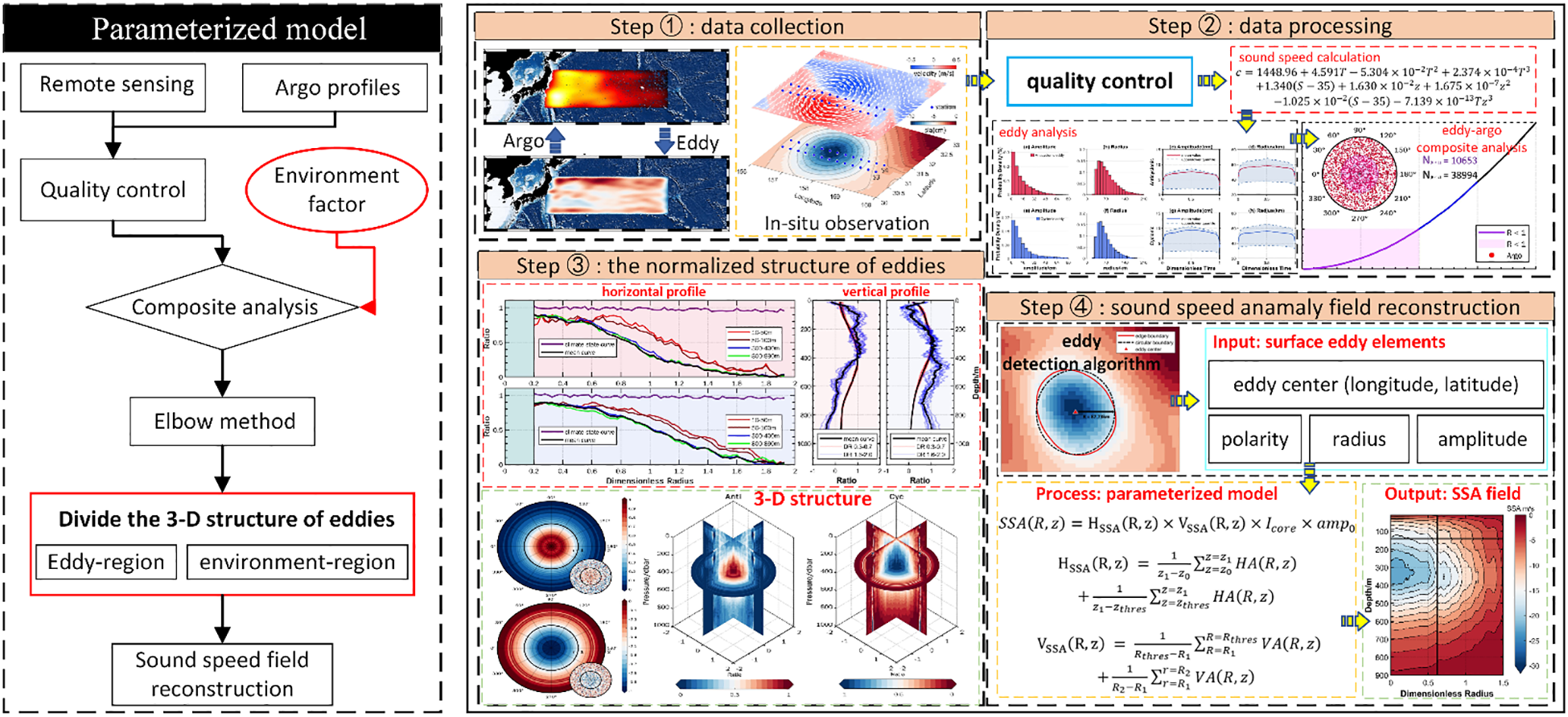
The flowchart for the development of the parameterized model.
The rest of the paper provides a more detailed presentation of the modeling and is organized as follows: the data and sound speed field reconstruction methodology are shown in section 2 and section 3, respectively. Section 4 is dedicated to the comparison of the reconstructed results with existing composite analysis methods and in situ observation experiments. We discuss and summarize the results in Section 5.
2 Data
Considering both the strength of mesoscale eddy activity and the availability of Argo float, the Kuroshio Extension (KE, 140°E-180°E, 30°N-40°N) has been chosen as the study area for this research. We evaluate the accuracy of proposed model using high resolution measured data from a cyclonic eddy in situ observation experiment. A detailed description of the data used is provided below:
2.1 Satellite altimeter data
The sea level anomaly (SLA) measured by satellite altimetry is derived from delayed-time altimeter gridded products distributed by CMEMS (Global Ocean Physics Reanalysis | Copernicus Marine Service). These data are originated from Sentinel-3A and Sentinel-6A and directly interpolated to the 0.25° grid at daily intervals. We extracted the data for the period from June 26 to June 30, 2014, to capture the sea surface height information.
2.2 Mesoscale eddy dataset
The Mesoscale Eddy Trajectory Atlas (META) dataset v.3.2 is distributed by Aviso+ (available at META3.2 DT). The dataset covers the period from January 1993 to February 2022. Each eddy includes information about the respective eddy’s amplitude, radius, center position, polarity type and boundaries which are identified at each time step from SLA maps using the contour threshold method proposed by Chelton (Chelton et al., 2011). Figure 2a displays the statistics of the number of eddy occurrences per 1° grid from 1993 to 2022 and topography in the KE, the abundance of mesoscale eddies in this area is clearly visible.
Figure 2
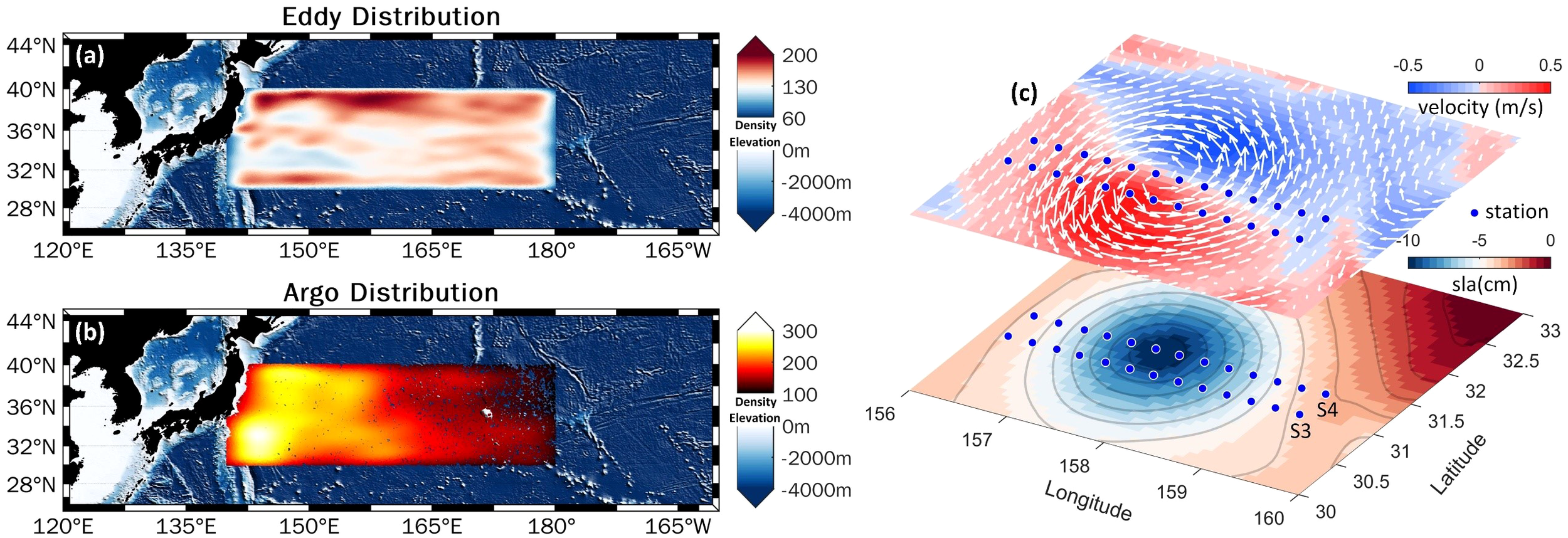
Distribution of (a) mesoscale eddies, (b) Argo and (c) the actually measured cyclonic eddy observation experiment. Density in (a) and (b) represent the number of occurrences of eddies and Argo profiles per 1° grid for the periods 1993-2022 and 1999-2023, respectively. Elevation in (a) and (b) mean the seabed topography. Upper layer in (c) is surface seawater flow field, the blue and red backgrounds represent the magnitude of the eastward and westward currents, respectively. Lower layer in (c) is sea surface characteristics, the blue region is where the cyclonic eddy is. Blue scatters in (c) are measured stations, including in situ temperature, salinity, pressure and underwater sound speed.
2.3 Argo profile
The statistics of Argo floats per 1° grid from 1999 to 2023 in the KE are shown in Figure 2b. The accumulation of Argo floats over the past 30 years has resulted in a substantial amount of temperature and salinity (T/S) profiles from the interior ocean, which can facilitate the reconstruction of eddy-induced sound speed fields. These global T/S profiles in upper 2000m are measured by Argo are available at ftp://ftp.ifremer.fr/ifremer/argo/geo/. Combined with the automatic preprocessing and quality control procedures implemented by the Argo data center, additional data filtering is performed to further enhance data quality in our paper:
-
Retain the selected Argo which can cover at least 10m-900m depth.
-
Retain the profiles with complete temperature, salinity and depth information.
-
Cubic spline interpolation is used to interpolate data at 1m intervals across the depth range of 10 to 1000 meters.
2.4 Climate state data
To better characterize the eddy-induced modifications in sound speed fields captured by Argo, the measured temperature/salinity profiles must be subtracted from the climate state data. The 3D monthly ocean climate state variables, mapped onto the regular 1/2° × 1/2° Mercator horizontal grid with 50 vertical levels, are provided by the Simple Ocean Data Assimilation (SODA) [available at SODA3.3.1 Download (SODA3.3.1 Download)].
2.5 Eddy observation experiment
A cyclonic eddy was observed over the area (156°-160°E, 30.33°-32°N) from June 26 to 30 during an in situ observation experiment conducted in 2014 (Zhang et al., 2019). The upper layer of Figure 2c represents the surface seawater flow field on June 28, 2014, the blue and red backgrounds represent the magnitude of the eastward and westward currents, respectively, and the lower layer means the sea level anomaly. The SLA derived from satellite altimeter data (in Section 2.1), and the flow field can be determined by calculating directly from SLA (Zhang et al., 2013). Route S3 and S4 in the Figure 2c delineate the in situ observation sites, which are strategically positioned to traverse the core of the eddy. The efficacy of the proposed model is evaluated by utilizing the sound speed data that has been directly measured along these Routes S3 and S4(Surveyed salinity and temperature data for a cyclonic eddy located in KE region).
3 Method
3.1 Sound speed anomaly
Based on the grid size of the climate state data provided by SODA3.3.1, the nearest neighbor interpolation (Huang et al., 2012) is used to obtain climate state temperature and salinity profiles at each Argo location. Measured sound speed profile (measured-SSP) and climate state sound speed profile (climate-SSP) can be calculated by using the nine-term empirical formula developed by Mackenzie, as shown in Equation 1 (Wang et al., 2021):
where , , and are temperature, salinity, and depth, respectively. This formula has a range of validity for temperatures between 2 and 30 degrees Celsius, salinity between 25 and 30 ppt, this is consistent with the thermohaline features of the upper 1000m of the ocean in the KE. Subsequently, sound speed anomaly (SSA) can be calculated by subtracting the climate-SSP from the measured-SSP.
3.2 Eddy detection
Bases on satellite altimeter observation, SLA-based (sea level anomaly-based) contour threshold method (Chelton et al., 2011; Xu et al., 2022) is used to detect surface eddies. Drawing on Chelton’s method and the statistical characteristics (this will be discussed in Section 4.1) of eddies in KE, we proceed with the following actions:
-
Step 1: For a cyclonic (anticyclonic) eddy, SLA caused by which must be below (high) a certain value. Precisely, anticyclonic eddy is 10cm, cyclonic eddy is -10cm.
-
Step 2: For a cyclonic (anticyclonic) eddy, at least one SLA minimum (maximum) exists.
-
Step 3: The sea surface height variation between an eddy’s center and boundary is defined as the eddy’s amplitude. The amplitude of each eddy is not less than 3 cm.
-
Step 4: Each eddy’s boundary is a closed contour.
-
Step 5: The horizontal scale of each eddy ranges from 50 to 300km.
Using the above procedures, we can identify mesoscale eddies from the single SLA remote sensing photograph. Further, similar to the reprocess of mesoscale eddies in META dataset (introduced in Section 2.2), we approximate the identified irregular eddy boundary as a circle, with the center of the circle representing the eddy’s center position and the radius representing the eddy’s horizontal scale. This process can be visualized in Figure 3. We will use two features of the eddy, amplitude and radius, as essential inputs to the proposed model.
Figure 3
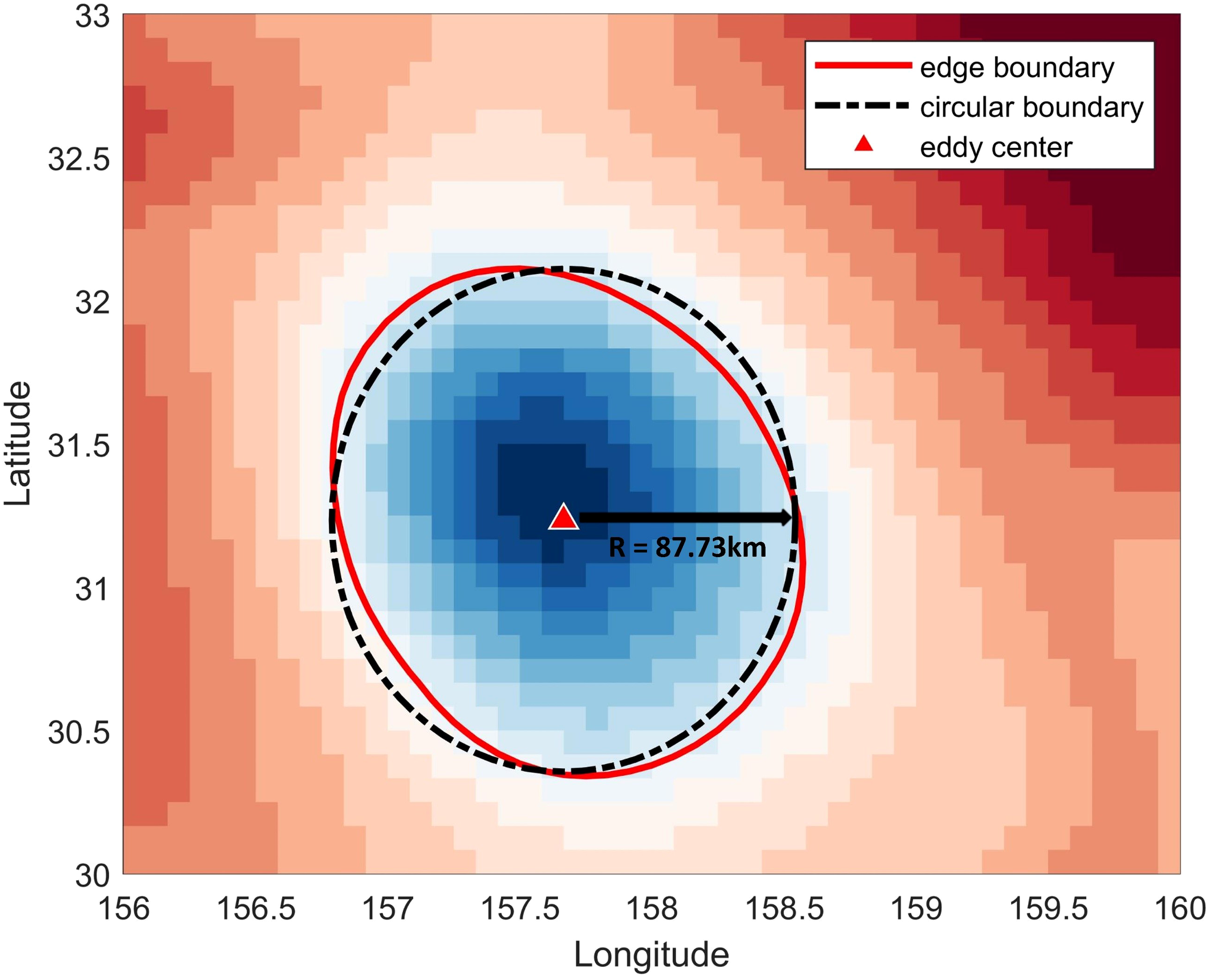
Schematic of eddy detection and reprocessing, background is SLA; the red solid line is the eddy’s boundary identified by SLA-based contour threshold method; the black dashed line is the approximate circular boundary; the red triangle is the eddy center.
3.3 Eddy-induced sound speed fields
The establishment of model is based on the fact that, despite the structure features and motion status varying over time, certain statistical properties of eddies remain comparatively stable. For example, the majority of eddies are found centrosymmetric (Chelton et al., 2011), and can rise Chlorophyll concentrations steadily (Zhao et al., 2021). By the same token, although the eddy-induced anomaly in sound speed fields can change with time and space as the eddy moves, it can be assumed that anomaly induced by eddies with certain amplitudes and horizontal scales are relatively stable in the KE region even throughout the global ocean (Chen et al., 2022). Therefore, we can consider the application of composite analysis (Chaigneau et al., 2011) to the eddies in the KE region, combining surface signals of eddies detected by satellite remote sensing and underwater sound speed profiles measured by Argo, to reconstruct eddy-induced sound speed fields.
The composite analysis in our study is based on the assumption that the 3D structure of the eddies can be seen axially symmetric and the acoustic properties in the eddy maintains relatively stable. However, in contrast to the approaches taken by previous scholars (Chen et al., 2022; Zhang et al., 2024; Zhao et al., 2021), we incorporate the influence of the external environment into the construction of the eddies’ composite structure. The procedure can be divided into four main steps:
Step 1: For each oceanic eddy, we construct the eddy-centered cylindrical coordinates (r, z), where r is the radial distance from the center of the eddy. Each Argo profile in the KE is matched with the closest eddy, the maximum difference of occurring time and distance between the Argo profile and the closest eddy center detected is less than 3.5 days and 2 eddy radius (), respectively.
Step 2: For each eddy-centered cylindrical coordinates, the eddy’s amplitude () and radius () are utilized to normalize the values and positions of the Argo profiles. This normalization establishes the relationship between the ocean surface eddy characteristics, and , and eddy-induced underwater characteristics. The process can be described by Equation 2 and Equation 3:
Where and represent the sound speed anomaly measured by Argo and the position of Argo, respectively, and denote the normalized SSA and the position of Argo profiles in a specific eddy-centered cylindrical coordinate. In this way, Argo profiles can be unified in the specific cylindrical coordinates (R, z).
Step 3: In dimensionless composite eddy-centered cylindrical coordinates (R, z), considering the vertical and horizontal structure of eddy-induced sound speed fields are separable (Chen et al., 2022), SSAamp at the composite eddy center and SSAamp at the depth where the max SSAamp is located are used to normalize SSAamp to obtain the horizontal () and vertical () pattern of the composite eddy, respectively, as shown in Equation 4 and Equation 5:
Where , in the interval [0,2], is the dimensionless horizontal distance between Argo profile and composite eddy center, is the SSAamp in the composite eddy center at z depth, which is in the range from 10 to 900m, and is the SSAamp in the depth at which the maximum SSAamp occurs.
After this treatment, the SSA at sample point () in the dimensionless eddy-centered cylindrical coordinates can be described by Equation 6:
Where is the SSAamp at the core depth (at which the maximum SSA occurs) of the composite eddy; is the amplitude, denoting eddy’s surface feature.
Step 4: Considering the eddy’s statistical characteristics, (Chen et al., 2022; Zhang et al., 2013) constructed the eddy composite structure by averaging the eddy’s horizontal and vertical patterns, as demonstrated by Equation 7 and Equation 8. In this research, this kind of model is referred to as the “average model” for brevity. The corresponding composite structure can be expressed as Equation 9:
Averaging the horizontal and vertical patterns of the eddy disregards the impact of the external environment on the eddy itself. However, many researches have indicated that the influence of the external environment on the eddy structure at different depths cannot be overlooked. Therefore, in contrast to their approach, we consider the impact of the external environment on the reconstruction of eddy-induced sound speed fields. In this research, this kind of model is referred to as the “environment factor-considering model” for brevity. The eddy’s vertical and horizontal composite structure this sentence should be modified as Equations 10–12:
and are horizontal and vertical component of composite eddy, respectively. Both of them are divided into two parts: one is the part that is more sensitive to the external environment properties, the other is the part that is more indicative of the intrinsic features of the composite eddy, which are Equations 13–16:
the part:
the part:
and denote the upper and lower boundaries of the depth, with values of and , respectively. and represent the left and right boundaries of the normalized radius, specifically and . The term refers to the threshold that distinguishes the part and part of the composite eddy that we derive by applying the threshold detection to horizontal and vertical components of the eddy, which will be discussed in more details in Section 4.
3.4 Evaluation index
In this study, we employ Mean Absolute Error (MAE) as the metric for evaluating the reconstruction performance of the parameterized model. Given a set of actual values and the corresponding reconstructed values , the calculation of mean absolute error is defined as follows:
To quantify the improvement in accuracy due to model optimization, we calculate the percentage reduction in error. Let the original mean absolute error be denoted as and the optimized mean absolute error as . The formula for calculating the percentage reduction in error is as follows:
Equation 17 calculates the absolute differences between the model reconstruction values and the actual observed values, and averages them to provide an intuitive measure of the model reconstruction error. Equation 18 offers a relative assessment of the performance improvement of the model before and after considering environment-factor, thereby allowing us to quantify the enhancement of the model’s effectiveness.
4 Result
4.1 Eddy features
Previous studies (Chelton et al., 2011; Chen et al., 2021; Stuhlmacher and Gade, 2020) demonstrated that mesoscale eddies in various sea regions display distinct surface characteristics. Therefore, it is necessary to acquire the statistics of surface eddies features (Figure 4) in the KE first to determine the most appropriate values of amplitude and radius as input parameters in eddy detection algorithm (in Section 3.2).
Figure 4
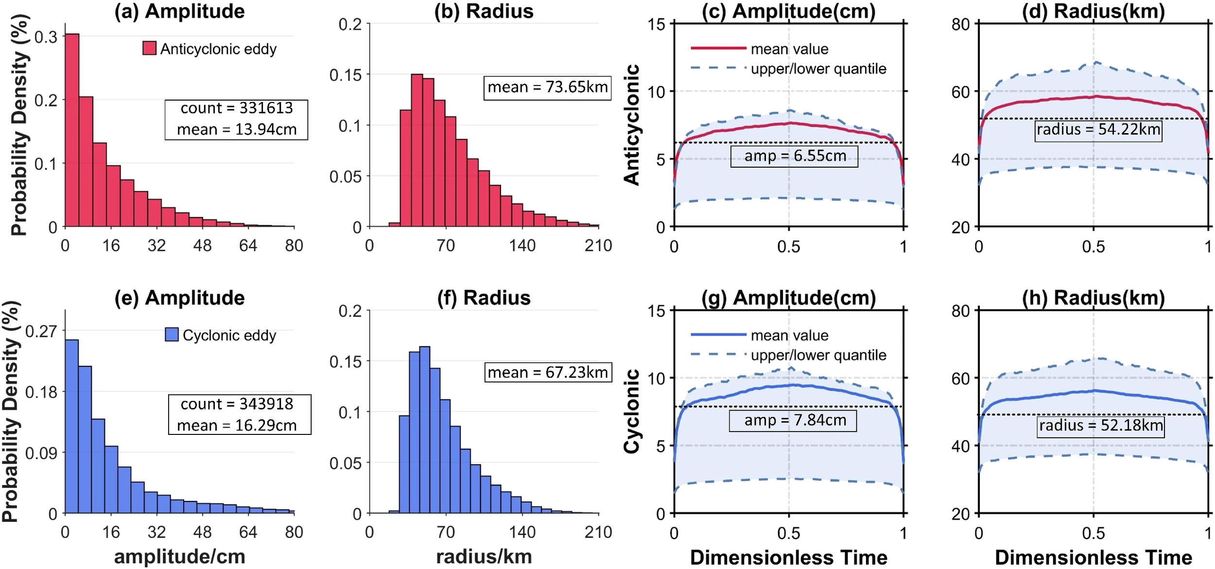
Histogram distributions of eddy amplitude (a, e), radius (b, f) and normalized life cycles of eddy amplitude (c, g), radius(d, h); the upper panel is anticyclonic eddy (red) and the bottom panel is cyclonic eddy (blue). (a, b, e, f) represent the probability density of eddies with different amplitudes/radius. The blue dashed lines in (c, d, g, h) represent the upper and lower quantiles of the amplitude/radius, and the black dashed lines represent the threshold that will be used as the most appropriate input parameters in eddy detection algorithm.
Between January 1993 and February 2022, a total of 331613 anticyclonic eddies and 343918 cyclonic eddies were identified in the KE. This indicates an average of 31 anticyclonic and 32 cyclonic eddies occurring daily in this region, which is characterized by vigorous eddy activity. Histograms of surface eddy features, specifically amplitude and radius, for cyclonic and anticyclonic eddies are presented in Figures 4a, b and Figures 4e, f, respectively. Cyclonic eddies tend to exhibit larger amplitudes and smaller radius, while anticyclonic eddies are characterized by smaller amplitudes and larger radius. Specifically, the average amplitude and radius for two types of eddies are 16.29 cm and 13.94 cm, and 67.23 km and 73.65 km, respectively.
By standardizing the surface characteristics of the two types of eddies according to their lifespans, we can reliably estimate the input parameter values. The resulting surface features of the eddies are displayed in Figures 4c, d, g, h, where the evolution pattern of amplitude and radius can be divided into three stages: the development phase, characterized by a rapid increase in both amplitude and radius; the maturity phase, during which surface features stabilize; and the dissipation phase, marked by a sharp decrease in eddy features. For our study, only eddies in the maturity phase are considered. We employ the elbow method (Syakur et al., 2018) to determine the average values of radius and amplitude at the beginning and end points of this phase. The results show that the normalized cyclonic eddy exhibits larger amplitude and smaller radius values at 7.84 cm and 52.18 km, respectively, while the normalized anticyclonic eddy has values of 6.55 cm and 54.22 km. These values are regarded as representative of the surface features of the eddies in the KE and will be used as reference threshold input values for the eddy detection method.
4.2 Eddy-argo composite analysis
To accurately model the eddy-induced sound speed fields we employ an enhanced composite analysis that takes into account the influences of external environmental factors. Cylindrical coordinates centered on the anticyclonic and cyclonic eddies are established, as shown in Figure 5.
Figure 5
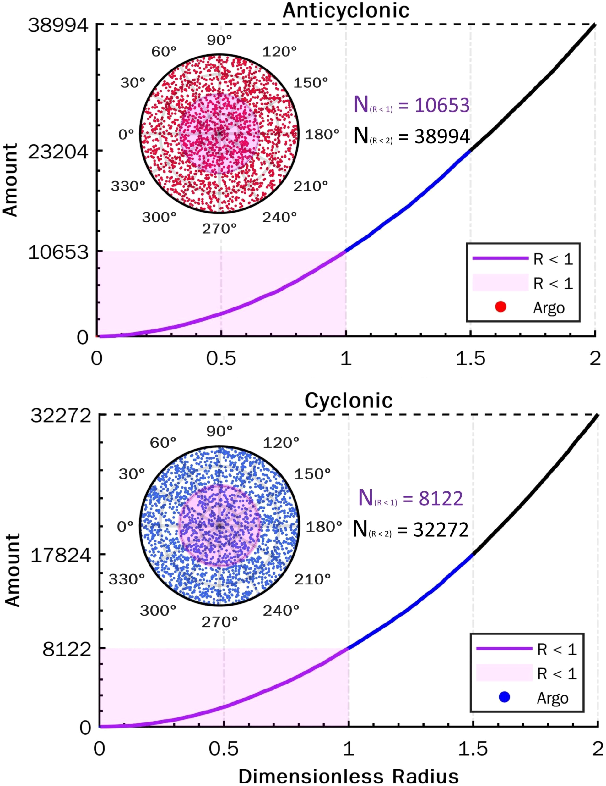
The upper panel and lower panel are anticyclonic (red) and cyclonic (blue) eddy, respectively. Circle in each panel is the constructed eddy-centered cylindrical coordinate, the purple boundary and black boundary represent regions with R<1 and R<2, respectively, scatter means the Argo profiles in the eddy-centered coordinate. The curve in each panel represents the cumulative number of Argo profiles in different regions with R ranging from 0 to 2, purple, blue and black means R in [0,1], [1,1.5] and [1.5,2], respectively.
The eddy-Argo composite analysis reveals that, for the anticyclonic (cyclonic) eddies, there are 38,994 (32,272) Argo profiles located within the eddy-centered coordinate region with (R< 2) and 10,653 (8,122) profiles within the region with (R< 1). These correspond to a ratio of eddies to Argo profiles of 0.12 (0.09) in the (R< 2) region, which is sufficient to support the robustness of the subsequent composite analysis (Chen et al., 2022; Zhang et al., 2013). The sound speed profiles measured by the Argo profiles are normalized by the eddies’ amplitude, and the normalized SSPs are presented in Figure 6.
Figure 6
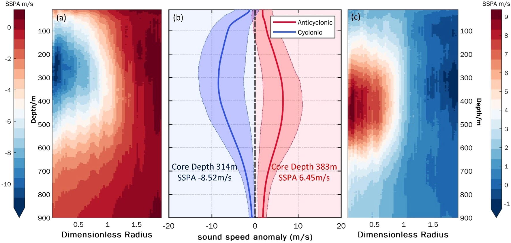
The sound speed profiles of composited eddy, the y-axis indicates depths from 10-900m. Vertical section of normalized cyclonic and anticyclonic eddy is displayed in (a, c), respectively, where the x-axis is dimensionless radius. Average SSA profile is displayed in (b), where blue indicates cyclonic eddy, red indicates anticyclonic eddy, the x-axis is normalized sound speed anomaly and the y-axis indicates depths from 10-900m. The red (blue) solid curve represents the mean SSA profile, the red (blue) shadow areas are the upper and lower quartiles of the mean SSA profile.
The sound speed profiles presented in Figure 6 demonstrates that the SSA curves—whether influenced by cyclonic (in Figure 6a) or anticyclonic eddies (in Figure 6c)—tend to initially increase and subsequently decrease with seawater pressure. This tendency can be attributed to both the non-local capture and local mixing effects (Frenger et al., 2015), stemming from the interaction between the eddy itself and the surrounding environment. Non-local capture optimizes the preservation of the acoustic characteristics of the water mass, while local mixing continuously alters the intrinsic properties of the eddy. This interaction manifests differently in eddies of varying polarity, at different seawater pressures, and across different oceanic regions.
In the ocean’s surface layer (approximately 0-200 m), the intrinsic properties of the eddy are diminished by external environmental factors such as heat transport at the air-sea interface and sea surface wind stress. This is illustrated in Figure 6b, where there is a gradual increase in SSA with seawater pressure. The influence of the ocean surface diminishes with depth, allowing eddies in the ocean’s middle layer to display their intrinsic properties while maintaining a relatively stable “bowl-shaped” structure. This stability is depicted in Figure 6b as a gradual decrease in SSA with increased seawater pressure.
By analyzing the top 10% of the largest SSA values and their corresponding depths, we can extract the core SSA of the eddy and its corresponding core depth. Consequently, we determine the core SSA and core depth of the normalized cyclonic and anticyclonic eddies to be -8.52 m/s at 314 m and 6.45 m/s at 383 m, respectively (denoted by the blue and red numbers in Figure 6b.
To derive the horizontal and vertical patterns of the composite eddies, we normalize the SSA measured by Argo against the SSA at the composite eddy core (R=0) at various depths, as well as the SSA at the core depth (z=zcore). This is illustrated in Figure 7.
Figure 7
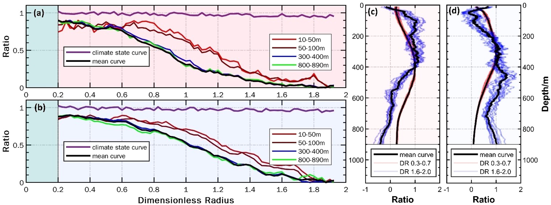
The horizontal structure (a, b) and vertical structure (c, d) of the composite eddy; for (a, b), the x-axis is dimensionless radius from 0 to 2 and the y-axis indicates the ratio of Argo-measured SSA to SSA at the eddy center at different depths; for (c, d), the x-axis is the ratio of Argo-measured SSA to SSA at the core depth and the y-axis indicates the pressure from 10-900dbar. (a, b) represent the horizontal structure of the anticyclonic and cyclonic eddies, respectively.
Taking the horizontal structure as an example, the significantly distinct attenuation pattern can be clearly observed in the horizontal structures of the climate state and the composite eddy. The climate state data remain almost parallel from the center of the eddy (R = 0.2) to the outer edges (R = 2), indicating that the oceanic sound speed background field is nearly constant over the 100-kilometer scale influenced by the eddy. In contrast, the horizontal structure of the composite eddy exhibits a gradual attenuation with increasing dimensionless radius (R). The disturbance of the background sound speed field caused by the eddy contributes to the differences observed between the horizontal structures of the climate state curve and those of the composite eddy. Consequently, the changes in the horizontal structure of the eddies with distance can reflect a decrease in the eddy-induced impact and an increase in the influence of the external environment.
Average horizontal structure aligns with the findings of previous studies, which indicate that the level ratio decays to 0.5 at (R = 1) and approaches 0 at (R = 2). Notably, in contrast to earlier research that regarded the horizontal structure of the eddy as decoupled from depth, our analysis of the eddy’s horizontal structure incorporates the influence of the external environment on the eddy’s structure at varying depths.
As shown in Figures 7a, b, the mean horizontal structure at depths of 10-50 m (red curve) and 50-100 m (brown curve) differs significantly from that at a depth range of 300-900 m. To address this disparity, (Zhang et al., 2013) and (Chen et al., 2022) assumed that the horizontal structure induced by the eddy is depth-independent, utilizing the average horizontal structure (black curve) from 0-900 m to represent the horizontal structure at various depths. This approach can be represented by Equation 7.
In contrast, for our study, we adopt a different approach. We divide the three-dimensional structure of the composite eddy into two distinct regions based on depth. The first is the environmental region, approximately 0-100 m, where the upper ocean environment is significantly influenced by surface features, such as wind. The second is the eddy region, approximately 100-900 m, which characterizes the essential features of the eddy itself. We believe that acoustic features of seawater in each region should exhibit a unique horizontal sub-structure, as they are each subjected to varying degrees of influence from surface ocean conditions and eddies.
To differentiate between environment-region and eddy-region, we introduce the coefficient of variance , which can be represented by Equation 19 and Equation 20:
Where represents the average error between the SSA of the composite eddy at depth and the average horizontal SSA. represents the average error between the SSA of the composite eddy at radius and the average vertical SSA. represents the number of layers in the horizontal structure, while indicates the number of layers in the vertical structure. The trend of horizontal and vertical variability with depth and radius is displayed in Figure 8:
Figure 8
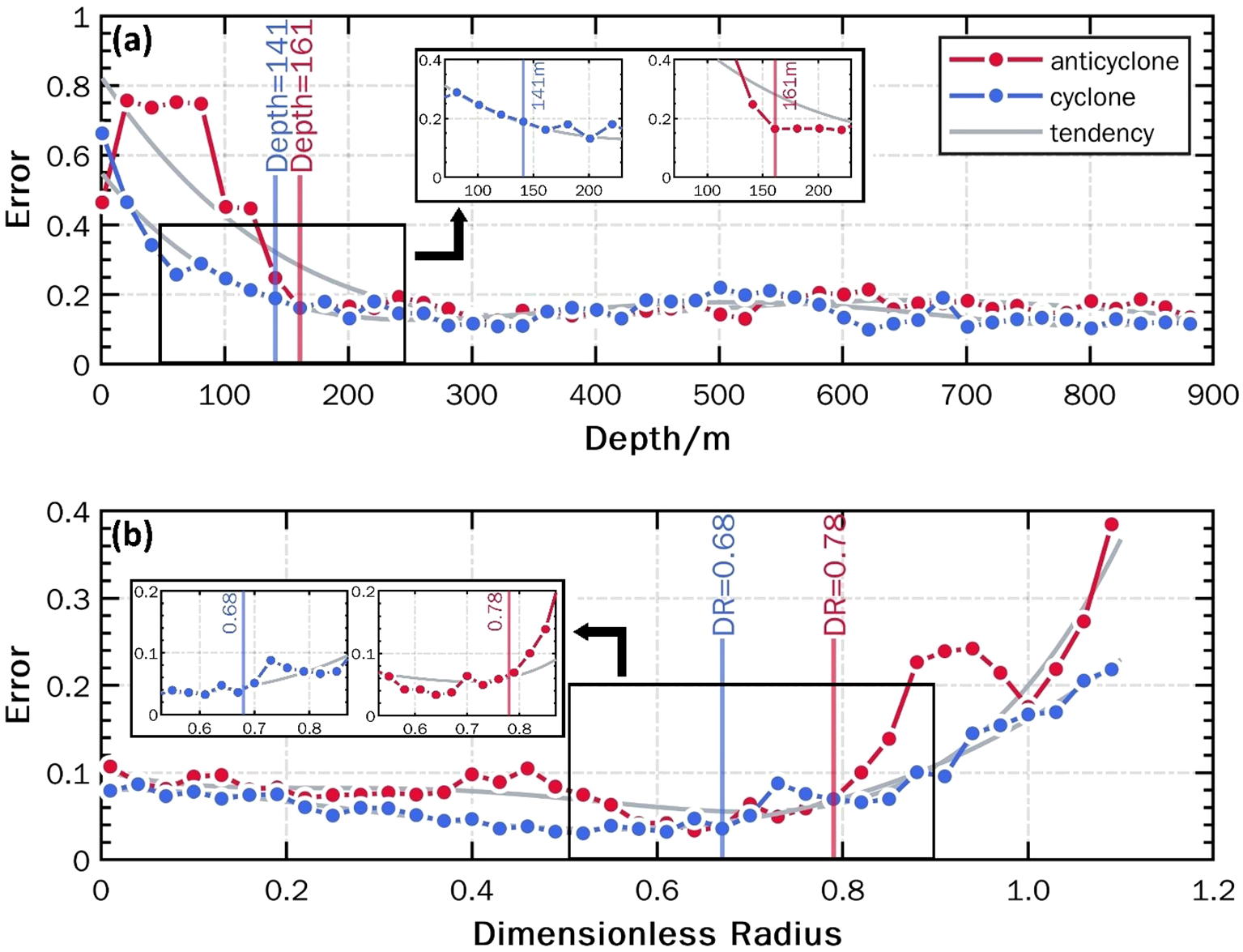
Horizontal (a) and vertical (b) structure error variation graphs. The blue and red curves in (a, b) represent the variation of error with depth in the cyclonic and anticyclonic eddies, respectively; the variation trend fitted with a fifth-degree polynomial function is shown by the gray curve. The x-axis in (a) is the depth ranging from 10 to 900m, the y-axis is the error and the black sub-boxes represent where the error varies most dramatically with depth. The vertical structure error variation is shown in (b), the x-axis is dimensionless radius, the y-axis is the error and the black sub-boxes represent where the error varies most dramatically with radius.
From Figure 8a, it can be observed that the difference between the horizontal structure and the average horizontal structure of the composite eddy decreases with increasing depth. This suggests that the influence of ocean surface environmental factors on the eddy is gradually diminishing. In the upper 250 meters, the error and its attenuation for the anticyclonic eddy are significantly greater than those for the cyclonic eddy. This discrepancy can be attributed to the fact that the anticyclonic eddy generates a descending flow, which facilitates the transmission of signals from the surface. In regions deeper than 250 meters, the error values for both anticyclonic and cyclonic eddies converge and show little variation with depth, indicating that this region is almost entirely unaffected by surface oceanic elements.
To accurately distinguish between the environment region and the eddy region, we utilized the elbow method to determine the boundary depth between the two. Prior to the elbow point, the rate of error reduction is quite dramatic, whereas beyond the elbow point, this rate becomes more gradual. As shown in the black sub-box of Figure 8a, we analyzed the trends of the curves alongside the vertical flow structure within the eddy, which allowed us to identify the critical depths of the horizontal structures for the anticyclonic and cyclonic eddies as 161 m and 141 m, respectively.
The differences in the vertical structure of cyclonic and anticyclonic eddies are illustrated in Figure 8b. In contrast to the horizontal structure of the eddy, the error in the vertical structure initially stabilizes before experiencing a dramatic increase. Within the range of 0 to 0.7, the error remains nearly constant, indicating that the composite eddy is relatively unaffected by external factors and maintains its intrinsic structure. However, in the range of 0.7 to 0.8, the error begins to rise gradually, signaling a transitional area where the characteristics of the eddy start to be influenced by the surrounding environment. In the range of 0.8 to 1, the error increases most dramatically, suggesting that the eddy is now significantly affected by external environmental factors. As illustrated in the black subframe of Figure 8b, we also employed the elbow rule to identify the boundary between the eddy itself and the external environment within the vertical structure. Our findings reveal that cyclonic and anticyclonic eddy exhibit anomaly increases in vertical structure error at radius of 0.68 and 0.78, respectively. We utilize these two values as thresholds for distinguishing between the two categories of vertical structure regions.
In conclusion, the thresholds for environment-region and eddy-region, used to distinguish between horizontal and vertical directions, are shown in Table 1:
Table 1
| Polarity | Depth (m) | Radius |
|---|---|---|
| Cyclonic eddy | 141 | 0.68 |
| Anticyclonic eddy | 161 | 0.78 |
Thresholds for environment-region and eddy-region.
Further, the environment factor-considering model can be established by Equations 21–23:
For cyclonic eddies, the threshold values are and , while for anticyclonic eddies, the threshold values are and . represents the normalized sound speed anomaly values at the cores of composite eddies with diverse polarities as shown in Figure 6. and can be pre-determined through composite analysis of eddy-Argo data as shown in Figure 7.
Therefore, in practical marine acoustics operations, it is possible to accurately reconstruct the underwater sound speed anomaly field within a depth range of up to 900 meters by simply inputting the amplitude, radius, and polarity parameters of the eddies identified through the eddy detection algorithm into the model (Equations 21–23), the influence of the input parameters on the reconstructed sound speed field is illustrated in Table 2. Subsequently, by overlaying this reconstructed sound speed anomaly field with the background climatic sound speed field, a high-precision reconstruction of the sound speed field induced by eddies can be accomplished. Moreover, it should be noticed that the model presented in our manuscript is specifically applicable to the Kuroshio Extension (KE, 140°E-180°E, 30°N-40°N) as it is based solely on Argo data and satellite remote sensing data from this region. To develop a parameterized model for the three-dimensional sound speed structure of eddies in other areas, one can employ the methods outlined in the previous sections by substituting the Argo and satellite remote sensing data with data from the area of interest.
Table 2
| Input | Attribute | Effect on model output |
|---|---|---|
| eddy center | longitude and latitude | determining the central position of the underwater sound speed field |
| radius | meters | determining the coverage area of the underwater sound speed field |
| polarity | anticyclonic or cyclonic | determining the type of the underwater sound speed field, with anticyclonic conditions resulting in positive sound speed anomalies and cyclonic conditions resulting in negative sound speed anomalies |
| amplitude | centimeters | determining the intensity of the underwater sound speed field; the greater the amplitude of the eddy, the stronger the resulting underwater sound speed field |
The influence of input parameters on the reconstructed sound speed field.
4.3 Model validation and comparison
To verify the reconstruction accuracy of the proposed model, we evaluate it with the observed cyclonic eddy presented in Section 2.5. By integrating data from satellite altimeters with the eddy identification method, we determined the amplitude and radius of the observed cyclonic eddy to be 3.82 cm and 87.77 km, respectively, with its center located at 31.23°E, 157.67°N.
As shown in Figure 9b, the underwater sound speed profiles inside and outside the eddy were recorded at 20 km intervals by the actual observed stations (Route S4, denoted as blue points). We interpolated the measured sound speed profiles to obtain the sound speed fields of this cyclonic eddy, as depicted in Figure 9a. The sound speed anomaly caused by the eddy exhibited a triangular cone-shaped distribution, with a maximum anomaly of -25 m/s occurring at a depth of 393 m (illustrated in Figure 9c).
Figure 9
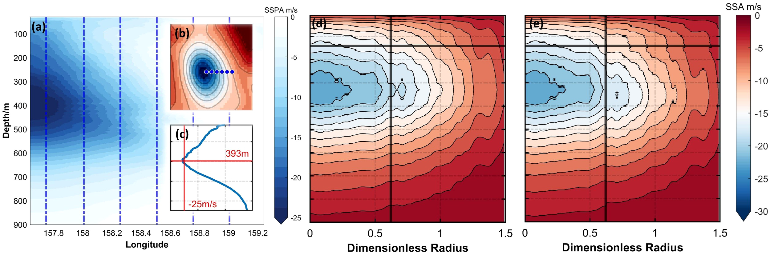
The observed eddy (a–c) and reconstructed eddy (d, e). (a) is the SSP of the observed cyclonic eddy, the x-axis is longitude and the y-axis is depth, the blue dotted line represents the profiles of in situ observed stations. (b) is the location of the eddy and the in situ stations, the blue dots represent the in situ stations corresponding to the blue dotted lines in (a), the x-axis represents the longitude, and the y-axis represents the latitude. (c) is sound speed anomaly curve at the center of the eddy, the x-axis is the value of sound speed anomaly (m/s), the y-axis is the depth. (d, e) are reconstructed eddy-induced sound speed fields using average structure model and the proposed model, respectively, the black lines represent the boundary between the environment-region and eddy-region, the x-axis is dimensionless radius and the y-axis is the depth.
Based on the obtained surface eddy information, we reconstructed the underwater sound speed field of the observed eddy using both the average structure model (Equations 7–9) and the environment factor-considering model (Equations 21–23) proposed in this study. The results are shown in Figure 9d and Figure 9e, respectively. The results show that the reconstructed sound speed anomalies of the eddy, achieved with the average model and the environment factor-considering model, exhibit errors of 2.9% and 2.7% within a dimensionless radius of 1, respectively. This indicates that the proposed model improves reconstruction accuracy by 6.77%. This phenomenon is primarily due to the environment-factor-considering model, which enhances reconstructed sound speed anomalies within the eddy region while diminishing them in the surrounding environment. For instance, as shown in Figures 9d, e, although the depths of the eddy core reconstructed by both models are nearly identical, the sound speed anomaly values in the core region differ significantly. The average model yields a sound speed anomaly of 22.01 m/s, whereas the environment factor-considering model reports a value of 22.92 m/s, which is closer to the actual sound speed anomaly in the eddy core (as shown in Figure 9a). Consequently, the latter model demonstrates superior reconstruction accuracy.
The improvement in the accuracy of underwater sound speed reconstruction will significantly enhance the precision of underwater sound propagation predictions. To evaluate this effect, we simulate the acoustic propagation in observed and reconstructed eddy using the Bellhop toolbox.
Referring to previous practices, we set the source frequency to 300 Hz, which is widely used in underwater acoustic engineering. The source depths were set at 315 m and 950 m, representing the core depth of the reconstructed eddy and the depth at which the acoustic channel is located, respectively. It should be noticed that, considering practical operational scenarios, we have set the sound source at 315 meters, corresponding to the reconstructed eddy, rather than at 393 meters, which pertains to the observed eddy. This decision is based on the fact that, during actual oceanographic missions, we can only obtain real-time information on the surface characteristics of observed eddies, and cannot access their underwater three-dimensional structures or core depths in real time. In this context, when using a parametric model to reconstruct the underwater three-dimensional structure, the sound source position can only be determined based on the reconstructed underwater three-dimensional structure of the parametric eddy. Additionally, simulation considers a deep-sea scenario, with a depth range set from 0 to 5000 m, and the horizontal distance corresponds to one eddy radius, which is 0 to 87.77 km. The output angle is limited to -20 to 20 degrees.
The simulation results are shown in Figure 10. We select the propagation loss at the intercept line corresponding to the depth of the sound source and the propagation loss of the entire sound speed field for comparative analysis, with the results presented in Table 3. The placement of the sound source significantly influences acoustic propagation, with the effect of the eddy on acoustic propagation becoming more pronounced as the sound source approaches the core region of the eddy. When the sound source is located at the core of the eddy (approximately 315 m), the accuracy of the propagation loss at the intercept line using the environment factor-considering model improves by about 0.71%. More significantly, the accuracy of the propagation loss for the entire sound speed field shows an improvement reaching up to 13.5%. This suggests that the environment factor-considering model has greater practical value in simulating acoustic propagation compared to the existing average model. The sound source, located at an estimated depth of 950 meters, predominantly sends its signals via the deep-sea sound channel. Simultaneously, the area most severely affected by the eddy extends to roughly 900 meters into the ocean, its influence gradually fading as the depth increases. As a result, for a sound source positioned at 950 meters, there is a negligible difference in the results yielded by the two models.
Figure 10
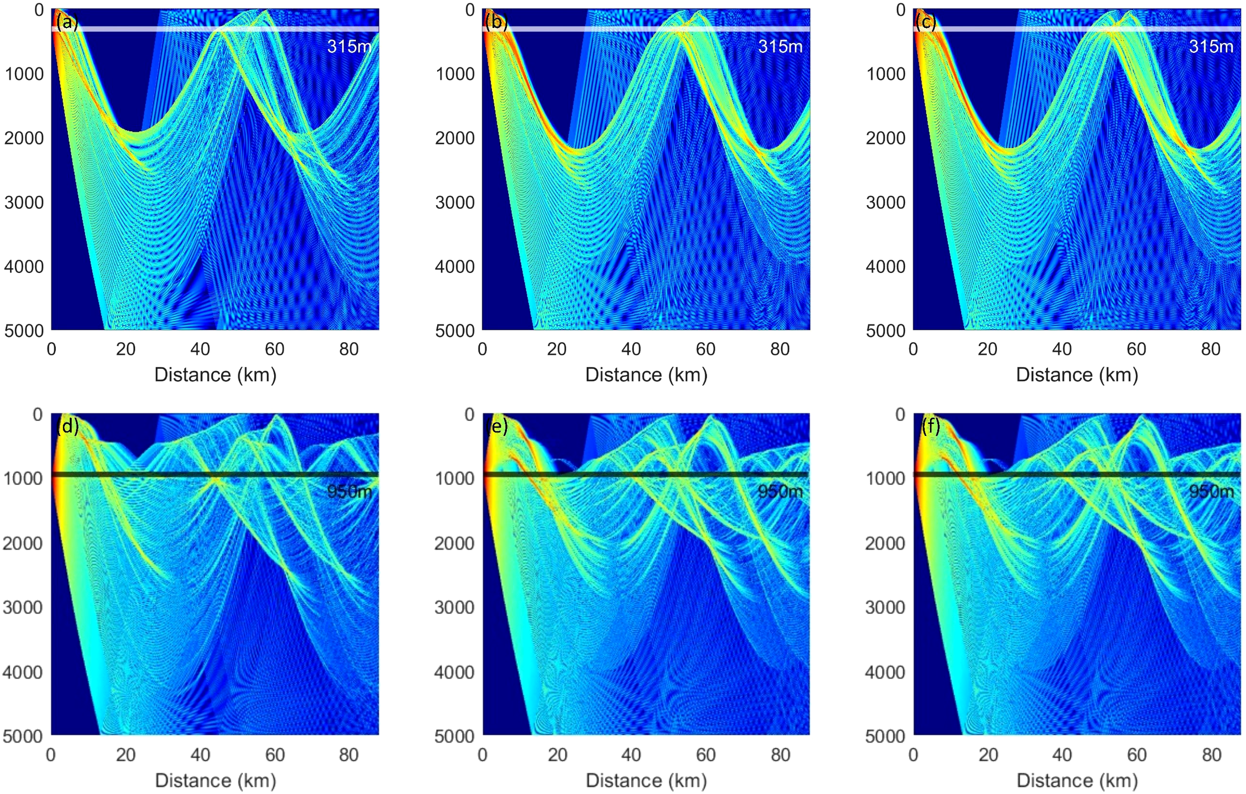
Comparison of underwater acoustic propagation characteristics of observed eddies and reconstructed eddies. (a, d) are transmission loss (TL) maps based on observed cyclonic eddy, (b, e) are TL maps based on composite eddy reconstructed by environment factor-considering model, (c, f) are TL maps based on composite eddy reconstructed by average model. The white and black lines represent different depths at which the source is located: 315m and 950m respectively, the x-axis is transmission distance, the y-axis is depth.
Table 3
| Scenario | Model Type | 315m | 950m |
|---|---|---|---|
| Line | The average model | 5.65 | 5.98 |
| The proposed model | 5.61 | 6.01 | |
| Accuracy improvement | +0.71% | -0.47% | |
| Field | The average model | 28.97 | 13.69 |
| The proposed model | 25.06 | 13.66 | |
| Accuracy improvement | +13.5% | +0.22% |
Transmission loss error characteristics.
Therefore, upon comparing the reconstructed results from the average model and the environment factor-considering model against the observed sound speed profile, we note that although the propagation loss calculated along the intercept line is comparable between the two models, there is a considerable discrepancy in the overall reconstruction accuracy of the entire sound speed field. Specifically, when utilizing the environment factor-considering model, the accuracy of the acoustic propagation loss calculation can be enhanced by an impressive 13.5%. This finding underscores the substantial practical value of the environment factor-considering model in predicting acoustic propagation.
5 Conclusion
To accurately predict underwater acoustic propagation, it is essential to establish a high-precision dynamic underwater sound speed fields in real-time. Various complex physical phenomena in the ocean, such as internal waves, oceanic fronts, and mesoscale eddies, are critical factors that must be considered in the process of constructing underwater sound speed fields. In this research, we propose an environment factor-considering model to parameterize the impact of eddies on the underwater sound speed field. The novel model leverages the advantages of satellite remote sensing technology, which offers near-real-time data and extensive spatial-temporal coverage, in conjunction with the reliability of Argo float observations, enabling the reconstruction of the underwater sound speed field in the presence of eddies on a time scale of just seconds.
The novel environment factor-considering model incorporates environmental factors into its framework to enhance the accuracy and efficiency of sound speed fields reconstruction, specifically reflected in the following aspects:
-
Compared to traditional numerical models and in situ observation experiments, the proposed model requires only the surface characteristics of eddies captured by satellite remote sensing as input—such as location, amplitude, radius, and polarity—to reconstruct the underwater acoustic environment within seconds.
-
Compared to the most commonly used acoustic field reconstruction methods, the environment factor-considering model demonstrates a 6.7% improvement in the accuracy of underwater sound speed reconstruction and a 13.5% improvement in the accuracy of acoustic propagation loss calculations.
In conclusion, this parameterized model can play a significant role in reducing costs and improving efficiency for high-precision underwater acoustic operations involving eddy occurrences, demonstrating substantial practical application value. Despite considering the influence of the external environment on the internal structure of eddies, the model still has many areas for improvement. For example, the model is based on the axisymmetric assumption of mesoscale eddies; however, the actual eddy structures in the ocean often exhibit anisotropy. These issues will be addressed in further research.
Statements
Data availability statement
The original contributions presented in the study are included in the article/Supplementary Material. Further inquiries can be directed to the corresponding author.
Author contributions
LX: Conceptualization, Data curation, Methodology, Validation, Visualization, Writing – original draft, Writing – review & editing. AZ: Supervision, Validation, Visualization, Writing – review & editing. XS: Conceptualization, Investigation, Supervision, Validation, Visualization, Writing – review & editing. JX: Funding acquisition, Visualization, Writing – review & editing. YL: Software, Validation, Visualization, Writing – review & editing. DC: Validation, Visualization, Writing – review & editing. LC: Resources, Software, Validation, Writing – review & editing.
Funding
The author(s) declare financial support was received for the research and/or publication of this article. This research was jointly supported by (National Natural Science Foundation of China), grant number (41706106).
Conflict of interest
The authors declare that the research was conducted in the absence of any commercial or financial 2 relationships that could be construed as a potential conflict of interest.
Generative AI statement
The author(s) declare that no Generative AI was used in the creation of this manuscript.
Publisher’s note
All claims expressed in this article are solely those of the authors and do not necessarily represent those of their affiliated organizations, or those of the publisher, the editors and the reviewers. Any product that may be evaluated in this article, or claim that may be made by its manufacturer, is not guaranteed or endorsed by the publisher.
Supplementary material
The Supplementary Material for this article can be found online at: https://www.frontiersin.org/articles/10.3389/fmars.2025.1588066/full#supplementary-material
References
1
Akulichev V. A. Bugaeva L. K. Morgunov Y. N. Solovjev A. A. (2012). Influence of mesoscale eddies and frontal zones on sound propagation at the Northwest Pacific Ocean. J. Acoustical Soc. America131, 3354–3354. doi: 10.1121/1.4708575
2
Browning D. G. Christian R. J. Petitpas L. S. (1994). A global survey of the impact on acoustic propagation of deep water warm core ocean eddies. J. Acoustical Soc. America95, 2880–2880. doi: 10.1121/1.409431
3
Browning D. G. Scully-Power P. D. Bannister R. W. Vastano A. C. (2005). Project ANZUS Eddy—Phase One: acoustic modeling of an ocean eddy. J. Acoustical Soc. America57, S65–S65. doi: 10.1121/1.1995359
4
Chaigneau A. Eldin G. Dewitte B. (2009). Eddy activity in the four major upwelling systems from satellite altimetry, (1992–2007). Prog. Oceanogr.83, 117–123. doi: 10.1016/j.pocean.2009.07.012
5
Chaigneau A. Le Texier M. Eldin G. Grados C. Pizarro O. (2011). Vertical structure of mesoscale eddies in the eastern South Pacific Ocean: A composite analysis from altimetry and Argo profiling floats. J. Geophys. Res. Oceans.116. doi: 10.1029/2011JC007134
6
Chelton D. B. Schlax M. G. Samelson R. M. (2011). Global observations of nonlinear mesoscale eddies. Prog. Oceanogr.91, 167–216. doi: 10.1016/j.pocean.2011.01.002
7
Chen C. Jin T. Zhou Z. (2019). Effect of eddy on acoustic propagation from the surface duct perspective. Appl. Acoustics150, 190–197. doi: 10.1016/j.apacoust.2019.02.019
8
Chen G. Yang J. Han G. (2021). Eddy morphology: Egg-like shape, overall spinning, and oceanographic implications. Remote Sens. Environ.257, 112348. doi: 10.1016/j.rse.2021.112348
9
Chen R. Thompson A. F. Flierl G. R. (2016). Time-dependent eddy-mean energy diagrams and their application to the ocean. J. Phys. Oceanogr.46, 2827–2850. doi: 10.1175/jpo-d-16-0012.1
10
Chen W. Zhang Y. Liu Y. Ma L. Wang H. Ren K. et al . (2022). Parametric model for eddies-induced sound speed anomaly in five active mesoscale eddy regions. J. Geophys. Res. Oceans.127 (8), e2022JC018408. doi: 10.1029/2022JC018408
11
Colosi J. A. Cornuelle B. D. Dzieciuch M. A. Worcester P. F. Chandrayadula T. K. (2019). Observations of phase and intensity fluctuations for low-frequency, long-range transmissions in the Philippine Sea and comparisons to path-integral theory. J. Acoustical Soc. America146, 567–585. doi: 10.1121/1.5118252
12
DeFerrari H. (2006). Predicting sonar performance using observations of mesoscale eddies. J. Acoustical Soc. America120, 3260–3260. doi: 10.1121/1.4788352
13
DeFerrari H. Olson D. (2003). The influence of mesoscale eddies on shallow water acoustic propagation. J. Acoustical Soc. America114, 2376–2376. doi: 10.1121/1.4777436
14
Dong C. You Z. Dong J. Ji J. Sun W. Xu G. et al . (2025). Oceanic mesoscale eddies. Ocean-Land-Atmos. Res. 4, 0081. doi: 10.34133/olar.0081
15
Ehlers S. Klein M. Heinlein A. Wedler M. Desmars N. Hoffmann N. et al . (2023). Machine learning for phase-resolved reconstruction of nonlinear ocean wave surface elevations from sparse remote sensing data. Ocean Eng.288, 116059. doi: 10.1016/j.oceaneng.2023.116059
16
Frenger I. Münnich M. Gruber N. Knutti R. (2015). Southern Ocean eddy phenomenology. J. Geophys. Res. Oceans.120(11), 7413–7449. doi: 10.1002/2015JC011047
17
Heaney K. D. Campbell R. L. (2016). Three-dimensional parabolic equation modeling of mesoscale eddy deflection. J. Acoustical Soc. America139, 918–926. doi: 10.1121/1.4942112
18
Henrick R. F. Siegmann W. L. Jacobson M. J. (1977). General analysis of ocean eddy effects for sound transmission applications. J. Acoustical Soc. America62, 860–870. doi: 10.1121/1.381606
19
Hirabayashi S. Sato T. Watanabe Y. Nishibori F. (2012). Numerical reproduction method of unsteady small-scale eddy field in the ocean. Ocean Eng.54, 196–205. doi: 10.1016/j.oceaneng.2012.06.020
20
Huang H. Cui C. Cheng L. Liu Q. Wang J. C. (2012). Grid interpolation algorithm based on nearest neighbor fast search. Earth Sci. Inf.5, 181–187. doi: 10.1007/s12145-012-0106-y
21
Jensen J. K. Hjelmervik K. T. Ostenstad P. (2012). Finding acoustically stable areas through empirical orthogonal function (EOF) classification. IEEE J. Oceanic Eng.37, 103–111. doi: 10.1109/JOE.2011.2168669
22
Li M. Liu Y. H. Sun Y. Y. Liu K. F. (2024). Quantitative analysis and prediction of the sound field convergence zone in mesoscale eddy environment based on data mining methods. Acta Oceanologica Sin.43, 110–120. doi: 10.1007/s13131-024-2328-5
23
Li H. Xu F. Wang G. (2022). Global mapping of mesoscale eddy vertical tilt. J. Geophys. Res. Oceans.127 (11), e2022JC019131. doi: 10.1029/2022JC019131
24
Lin R. Cao J. Xiao J. Yu C. Liu C. Yao B. et al . (2023). Dynamic modeling and switching analysis of all-attitude multimode underwater vehicle for multidimensional data acquisition. Ocean Eng.286, 115550. doi: 10.1016/j.oceaneng.2023.115550
25
Lü L.-G. Qiao F. Chen H.-X. Yuan Y.-L. (2006). Acoustic transmission in the cold eddy in the southern East China Sea. J. Geophys. Res. Oceans. 111. doi: 10.1029/2005JC003162
26
Ma X. Zhang L. Xu W. Li M. Zhou X. (2024). A mesoscale eddy reconstruction method based on generative adversarial networks. Front. Mar. Sci.11, 1411779. doi: 10.3389/fmars.2024.1411779
27
Nie R. He T. Fan J. Zhao K. Wang B. (2024). Fast prediction of the long-range structural acoustic radiation in the stratified ocean. Ocean Eng.314, 119673. doi: 10.1016/j.oceaneng.2024.119673
28
Ramp S. R. Colosi J. A. Worcester P. F. Bahr F. L. Heaney K. D. Mercer J. A. et al . (2017). Eddy properties in the subtropical countercurrent, Western Philippine sea. Deep Sea Res. Part I: Oceanographic Res. Papers125, 11–25. doi: 10.1016/j.dsr.2017.03.010
29
Scully-Power P. D. Nysen P. A. (2005). A new definition for acoustic transition range with application to oceanic eddies. J. Acoustical Soc. America64, S75–S76. doi: 10.1121/1.2004361
30
Stuhlmacher A. Gade M. (2020). Statistical analyses of eddies in the Western Mediterranean Sea based on Synthetic Aperture Radar imagery. Remote Sens. Environ.250, 112023. doi: 10.1016/j.rse.2020.112023
31
Syakur M. A. Khotimah B. K. Rochman E. M. S. Satoto B. D. (2018). Integration K-means clustering method and elbow method for identification of the best customer profile cluster. IOP Conf. Series: Materials Sci. Eng.336, 12017. doi: 10.1088/1757-899X/336/1/012017
32
Vazquez H. J. Cornuelle B. D. Worcester P. F. Dzieciuch M. A. Colosi J. A. Nash J. D. (2023). Using long-range transmissions in the Beaufort Gyre to test the sound-speed equation at high pressure and low temperature. J. Acoustical Soc. America154, 2676–2688. doi: 10.1121/10.0021973
33
Wang Z. Xu J. Zhang X. Lu C. Jin K. Zhang Y. (2021). Flow-dependent modeling of acoustic propagation based on the DG-FEM method. J. J. Atmospheric Oceanic Technol.38, 1823–1832. doi: 10.1175/JTECH-D-21-0001.1
34
Xi Q. Fu Z. Xue M.-A. Zou M. Zheng J. (2023). Analysis of underwater acoustic propagation induced by structural vibration in arctic ocean environment based on hybrid FEM-WSM solver. Ocean Eng.287, 115922. doi: 10.1016/j.oceaneng.2023.115922
35
Xiao Y. Li Z. Sabra K. G. (2018). Effect of mesoscale eddies on deep-water sound propagation. J. Acoustical Soc. America143, 1873–1874. doi: 10.1121/1.5036149
36
Xu L. Gao M. Zhang Y. Guo J. Lv X. Zhang A. (2022). Oceanic mesoscale eddies identification using B-spline surface fitting model based on along-track SLA data. Remote Sensing14 (22), 5713. doi: 10.3390/rs14225713
37
Xu W. Zhang L. Li M. Ma X. Li M. (2024a). Data-driven analysis of ocean fronts’ Impact on acoustic propagation: process understanding and machine learning applications, focusing on the kuroshio extension front. J. Mar. Sci. Eng.12, 2010. doi: 10.3390/jmse12112010
38
Xu W. Zhang L. Li M. Ma X. Wang H. (2024b). A physics-informed machine learning approach for predicting acoustic convergence zone features from limited mesoscale eddy data. Front. Mar. Sci.11, 1364884. doi: 10.3389/fmars.2024.1364884
39
Xue Y. Yue L. Ding R. Zhu S. Liu C. Li Y. (2023). Influencing mechanisms of gas bubbles on propagation characteristics of leakage acoustic waves in gas-liquid two-phase flow. Ocean Eng.273, 114027. doi: 10.1016/j.oceaneng.2023.114027
40
Zhang Y. Chen X. Dong C. (2019). Anatomy of a cyclonic eddy in the kuroshio extension based on high-resolution observations. Atmosphere10 (9), 553. doi: 10.3390/atmos10090553
41
Zhang G. Chen R. Li L. Wei H. Sun S. (2023). Global trends in surface eddy mixing from satellite altimetry10. doi: 10.3389/fmars.2023.1157049
42
Zhang Z. Wang G. Wang H. Liu H. (2024). Three-dimensional structure of oceanic mesoscale eddies. Ocean-Land-Atmos. Res.3, 0051. doi: 10.34133/olar.0051
43
Zhang Z. Zhang Y. Wang W. Huang R. X. (2013). Universal structure of mesoscale eddies in the ocean. Ocean-Land-Atmos. Res.40, 3677–3681. doi: 10.1002/grl.50736
44
Zhao D. Xu Y. Zhang X. Huang C. (2021). Global chlorophyll distribution induced by mesoscale eddies. Remote Sens. Environ.254, 112245. doi: 10.1016/j.rse.2020.112245
45
Zheng Y. Lin J. Chen X. (2024). Application of fluctuations in the sound field in inversion of internal solitary wave phase speed. Ocean Eng.305, 117867. doi: 10.1016/j.oceaneng.2024.117867
Summary
Keywords
parameterized model, environment factor-considering, oceanic eddy, underwater sound speed fields, three-dimensional structure reconstruction
Citation
Xu L, Zhang A, Sun X, Xu J, Liu Y, Chen D and Chen L (2025) A parameterized model for the real-time reconstruction of underwater sound speed fields in oceanic eddy environment. Front. Mar. Sci. 12:1588066. doi: 10.3389/fmars.2025.1588066
Received
05 March 2025
Accepted
24 July 2025
Published
13 August 2025
Volume
12 - 2025
Edited by
Yimian Dai, Nanjing University of Science and Technology, China
Reviewed by
Miguel Angel Ahumada-Sempoal, University of the Sea, Mexico
Chengbo Wang, University of Science and Technology of China, China
Updates
Copyright
© 2025 Xu, Zhang, Sun, Xu, Liu, Chen and Chen.
This is an open-access article distributed under the terms of the Creative Commons Attribution License (CC BY). The use, distribution or reproduction in other forums is permitted, provided the original author(s) and the copyright owner(s) are credited and that the original publication in this journal is cited, in accordance with accepted academic practice. No use, distribution or reproduction is permitted which does not comply with these terms.
*Correspondence: Xuehai Sun, xhsun_nsa@163.com
Disclaimer
All claims expressed in this article are solely those of the authors and do not necessarily represent those of their affiliated organizations, or those of the publisher, the editors and the reviewers. Any product that may be evaluated in this article or claim that may be made by its manufacturer is not guaranteed or endorsed by the publisher.