Spatio-temporal variability of San Francisco Bay Plume from space

As brackish turbid waters exit San Francisco Bay, one of the largest estuaries in the U.S. West Coast, they form the San Francisco Bay Plume (SFBP), which spreads offshore and influences the Gulf of the Farallones (GoF), an ecologically significant region in the California Current System that is also home to three National Marine Sanctuaries. This paper provides the first observationally based investigation of the spatio-temporal variability of the SFBP, using a plume tracking algorithm applied to more than two decades (2002-2023) of ocean color data from the Moderate Resolution Imaging Spectroradiometer (MODIS) sensor onboard satellites Aqua and Terra. The turbid SFBP spreads radially, extending 10-20 km offshore around 50% of the time, and during extreme discharge events (<1% of the time), the plume can reach nearly 60 km offshore to the shelf break. The greatest variability in frequency of plume occurrence was observed 10-20 km offshore and it was largely explained by the seasonal cycle (80% of total variance), linked primarily to seasonal changes in river discharge. Largest plume areas (determined by summing up all pixel areas weighted by their respective fraction of plume occurrence) were observed during winter and smallest during summer, occupying on average 24% and 1.5% of GoF area, respectively. Beyond 20-30 km offshore, variability in frequency of plume occurrence was dominated by the intraseasonal band (50-80% of total variance), attributed to plume response to synoptic wind-forcing and/or filaments and eddies, while the interannual band played a secondary role in the plume variability (<20% of total variance). Finally, a multivariable linear regression model of the turbid SFBP area was created to explore the potential predictability of the plume’s influence in the GoF. The model included the annual and semi-annual cycles and discharge anomalies (deseasoned and detrended), and despite its simplicity, it explained over 78% of total variance of the turbid SFBP area. Therefore, it could be a useful tool for scientists and stakeholders to better understand how management actions on freshwater supply can have consequences offshore beyond the Golden Gate and help guide future management decisions in this ecologically important region.

1 Introduction

River plumes are key components of the circulation in a great number of continental shelves around the world (Hill, 1998). The buoyancy input from estuarine outflow affects the shelf hydrographic properties, generating sharp density fronts and increasing the ambient stratification. These changes can lead to the generation of swift geostrophic currents (e.g. Pimenta et al., 2011; Mazzini et al., 2014), affect internal wave propagation (e.g. Nash and Moum, 2005), and modify small-scale processes in the ocean, such as turbulence and mixing (e.g. Dzwonkowski et al., 2018; Fisher et al., 2018). The profound impact of river plumes is not only restricted to the physical dynamics, but they also influence geological, chemical, and biological processes as they provide a conduit for the delivery of estuary and river-born substances and materials to the coastal ocean, including nutrients, phytoplankton, larvae, sediments, micro- and macro-plastics as well as other pollutants. Understanding how river plumes vary spatially and temporally is therefore critical for assessing their influence and impact on the coastal ocean.

River plumes generally exhibit short time scales of variability, and can occupy vast surface areas. Thus, quasi-synoptic in situ measurements of their full extent and capturing their temporal evolution are practically impossible, and therefore have been typically limited to small portions of the plume over limited times (e.g. Lentz and Largier, 2006; Yankovsky, 2006; MacDonald et al., 2007; Chant et al., 2008; Horner-Devine et al., 2009; Kakoulaki et al., 2014; Mazzini et al., 2014, 2019; Mazzini and Chant, 2016; Yankovsky and Voulgaris, 2019). More recently, satellite remote sensing techniques have emerged as valuable tools for mapping plumes, and have yielded critical insight into these multiscale flow structures. River plume waters have distinct optical properties from those in the adjacent coastal ocean due to their contrasting and complex biogeochemical compositions (Schofield et al., 2004), they often carry large concentrations of organic matter and suspended sediments, which tend to give them a green-yellow-brownish color (e.g. Klemas, 2012). Several studies have taken advantage of this fact and utilized ocean color satellite remote sensing to investigate river plumes throughout the globe (e.g. Warrick et al., 2004; Nezlin and DiGiacomo, 2005; Dzwonkowski and Yan, 2005; Thomas and Weatherbee, 2006; Nezlin et al., 2008; Palacios et al., 2009; Shi and Wang, 2010; Saldias et al., 2016; Mendes et al., 2014; da Silva and Castelao, 2018; Speiser and Largier, 2024; Martineac et al., 2024; Dykstra et al., 2024; Castelao and Medeiros, 2025). Now, with the Moderate Resolution Imaging Spectroradiometer (MODIS) onboard satellites Aqua and Terra exceeding two decades in space, providing high-resolution (~1km) multi-spectral ocean color measurements with daily global coverage, it is becoming possible to explore variability of river plumes on interannual time scales.

In this study, we use 21 years of MODIS data (2002-2023) and a plume tracking algorithm (Nezlin and DiGiacomo, 2005) to investigate spatiotemporal variability of the turbid San Francisco Bay Plume (SFBP), an understudied, human-impacted river plume, that influences an extremely complex and ecologically important region, the Gulf of the Farallones (GoF), located in the California north central coast (Figure 1). Our goal is to characterize the spatial variability of SFBP from intraseasonal (monthly) to interannual time scales, assess the influence of the plume in the GoF by quantifying the surface area and fraction of the gulf occupied by the plume, and investigate the relationship between the plume and major forcing mechanisms, including river discharge, winds and water level.

Figure 1

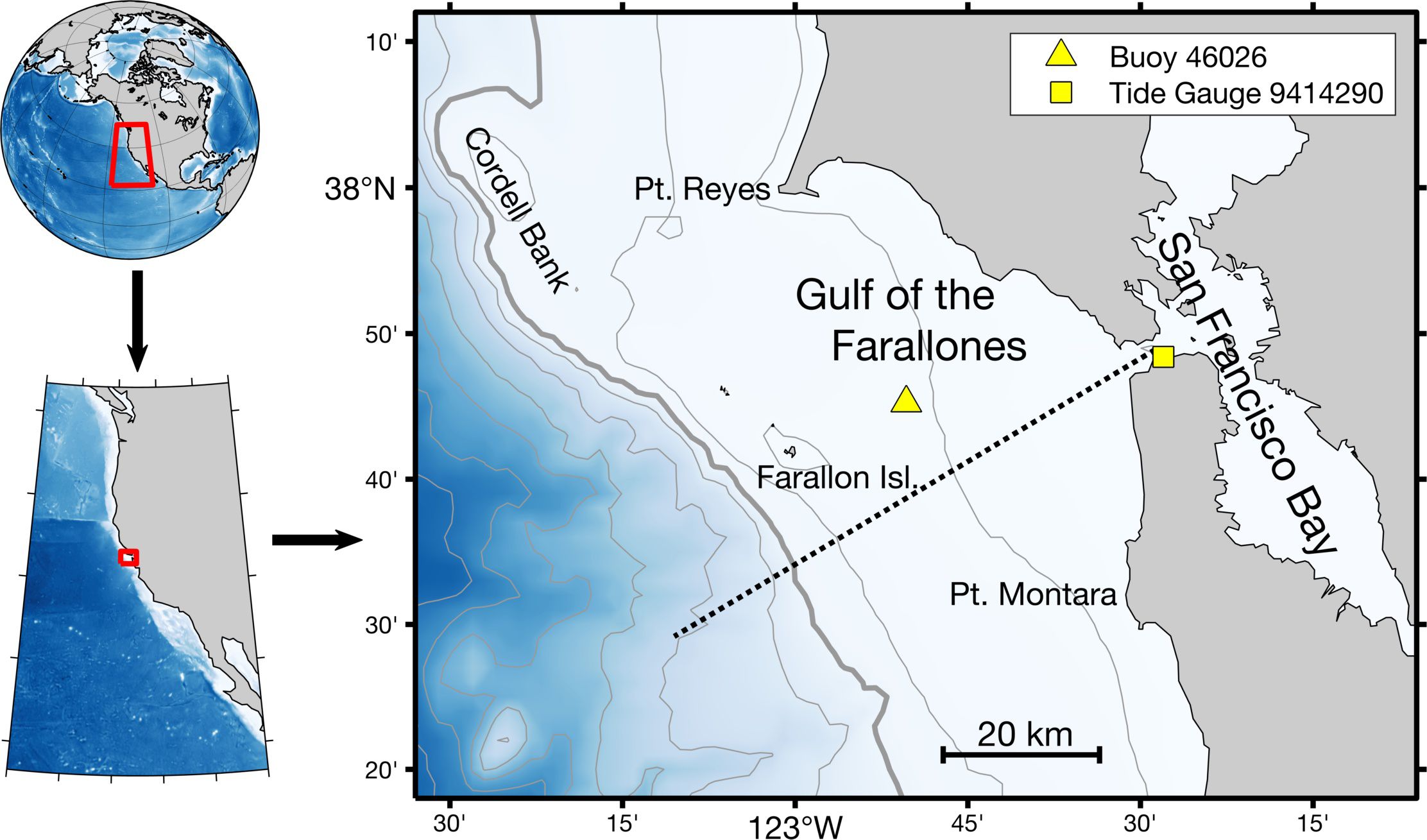
Figure 1. Map of the study area, depicting the Gulf of the Farallones adjacent to the San Francisco Bay estuary, located in California North Central Coast. Yellow symbols denote the location of wind measurements from buoy 46026 (triangle) and water level measurements from tide gauge 9414290 (square). The dashed line indicates the transect used for constructing Hovmöller diagrams presented in Figures 6, 8. Isobaths of 50, 100, 200, 500, 1000, 1500, 2000, 2500, 3000 are shown as gray contours, with a thicker contour denoting the 200 m isobath, highlighting the shelf break.

1.1 San Francisco Bay Plume and the Gulf of the Farallones

San Francisco Bay is one of the largest estuaries on the U.S. West Coast, located on the north central coast of California. It receives water from the Sacramento-San Joaquin river system, which drains approximately 40% of the California area (Kimmerer, 2004). The region has a Mediterranean climate, characterized by a winter wet season and summer dry season. The freshwater input to the San Francisco Bay estuary follows the seasonal precipitation pattern, despite being largely altered by humans. Discharge magnitudes are highly variable, ranging between 1,000-10,000 m³/s during winter and early spring and between 100-300 m³/s during summer and fall.

San Francisco Bay is a highly urbanized estuary (Conomos, 1979) where the population grew from 2.7 million in 1950 to 7.6 million in 2024 (Bay Area Census, 2025). Because of the landscape setting of the bay, situated between important cities such as San Francisco, Richmond, San Jose (Silicon Valley) and Oakland, the anthropogenic influence is massive, where industrial, commercial and agricultural wastes are delivered to bay waters through land runoff, groundwater, atmospheric deposition and municipal sewage. Understanding the impact of these anthropogenic contaminants is crucial for proper management of not only the San Francisco Bay but also for the adjacent coastal region, the GoF, and beyond.

The GoF lies west of the Golden Gate bridge and encompasses the continental shelf region bounded by Pt. Reyes (38.0°N) to the north, Pt. Montara (37.5°N) to the south, and offshore by the shelf break (Figure 1). The shelf is nearly 50-60 km wide, over twice the average shelf width of the broad region spanning from Oregon to the north and Point Conception, California, to the south, where the typical shelf width is around 20 km. GoF is an important upwelling hotspot, with some of the highest levels of nutrients and productivity in the California Current System and a large ecological diversity of pelagic and benthic communities, including the largest seabird breeding colony along the U.S. West Coast, important breeding sites for marine mammals, large aggregations of white sharks, and valuable commercial and recreational fisheries (Wilkerson et al., 2006; Wang et al., 2024). The GoF domain includes the Golden Gate Biosphere Reserve, a network of three National Marine Sanctuaries (Greater Farallones, Cordell Bank and Monterey Bay) managed by the National Oceanic and Atmospheric Administration (NOAA), and 25 State Marine Protected Areas.

As the brackish and turbid estuarine waters exit San Francisco Bay through the Golden Gate and enter the GoF, they form the San Francisco Bay Plume (SFBP). Some of the earliest studies of SFBP happened as early as the 1970’s (e.g. Carlson and McCulloch, 1974), but since then, limited observational efforts have been conducted to better understand the behavior of the plume, and therefore little is still known about its characteristics, variability and dynamics (Zhou et al., 2023). In the vicinity of the Bay mouth, currents are largely driven by tides (Gough et al., 2010; Fram et al., 2007), while farther offshore the variability of surface currents is dominated by subtidal time scales, with mean seasonal circulation over the shelf generally following classical Ekman response to wind-forcing (Gough et al., 2010), superposed by a complex meso- and sub-mesoscale eddy field (Steger et al., 2000). Buoyancy forcing from the SFBP and flow-topography interactions, particularly around Pt. Reyes, contribute to the complexity of the circulation in the GoF and surrounding areas. Winds in the region are characterized by three different seasons (García-Reyes and Largier, 2012): “Upwelling Season” (April-June) with strong equatorward (upwelling-favorable) winds and large standard deviation (due to frequent reversals); a “Relaxation Season” (July-September) with weak equatorward winds and low variability; and a “Storm Season” (December-February) characterized by weak mean wind stress but large variability, with remaining months being transitional, shifting to different seasons from year to year due to interannual variability.

2 Materials and methods

2.1 Time series of discharge, winds and water level

Daily information of river discharge was obtained from the Dayflow model of the Sacramento-San Joaquin Delta hydrology produced and made available by California Department of Water Resources. The “Net Delta Outflow” product, which will be simply referred to as discharge, was selected for this study. This product represents 93% of the freshwater inflow to SF Bay, and is calculated by the Dayflow model using river inflow, precipitation, evaporation, water export and consumptive usage of water across the Delta. Data availability and a detailed description of Dayflow can be found at: https://data.cnra.ca.gov/dataset/dayflow. Freshwater inflow from the Delta travels approximately 75 kilometers through Northern and Central San Francisco Bay before reaching the ocean. This region of the Bay is a partially mixed, microtidal estuary, where water residence times vary seasonally—from just a few days during periods of high winter river discharge to several months during the dry summer season (Walters et al., 1985).

Hourly values of wind speed and direction were obtained from buoy 46026 (37°45.23’ N, 122°50.33’ W) from NOAA’s National Data Buoy Center (NDBC), located near the center of the GoF, 33.3 km west of San Francisco (Figure 1). Speed and direction were transformed into zonal and meridional components, and used to compute wind stress following Large and Pond (1981). A 40-hour cut off low-pass filter was applied to those components in order to eliminate diurnal and other high frequency variability, and data were binned to daily values. Finally, the wind stress was rotated into along- and cross-shelf direction, determined by the direction of maximum variance (39.36° counterclockwise from true north) and minimum variance (39.36° counterclockwise from true east), respectively. Nearly 10.4% of the time series had missing values, which were mostly filled by regressing significantly correlated wind observations from along- and cross-shelf windstresses from adjacent NDBC stations 46012 (37°21.3’ N, 122°52.8’ W, off Half Moon Bay; not shown) and 46013 (38°14.1’ N, 123°19.0’ W, off Bodega Bay; not shown), located 44.4 southwest and 88.9 km northwest from San Francisco, respectively. The resulting wind stress time series had less than 0.5% of remaining gaps.

Water level information, used here as a proxy for pressure gradients, was obtained from hourly measurements recorded at NOAA tide gauge station 9414290 (37°48.4’ N, 122°28.0’ W), inside San Francisco Bay, located nearly 1.1 km from the Golden Gate (Figure 1). Water level time series was detided using harmonic analysis (removing six major constituents: M2, K1, O1, S2, N2 and P1) and subsequently low-pass filtered with a 40-hour cut off, similar to wind stress, and data were binned to daily values. Less than 0.3% of gaps present in the time series were filled by regressing significantly correlated water level observations from NOAA station 9415020 (37° 59.7 N, 122° 58.4 W, at Point Reyes; not shown), located 47 km northwest of San Francisco.

Finally, discharge, along- and cross-shelf wind stress, and water level were averaged to monthly values. Their respective anomalies were then calculated by subtracting their seasonal cycles, estimated through harmonic analysis using annual and semi-annual cycles, and subsequently removing their long-term trends through linear regression. These anomalies time series were then used to investigate their potential relationship to SFBP.

2.2 MODIS data

MODIS Level 1A (L1A) images from satellites Aqua and Terra covering the GoF and surrounding region (swaths between 37.2-38.4°N and 123.8-122°W) were obtained from the NASA Ocean Biology Processing Group (https://oceancolor.gsfc.nasa.gov/) during the period of July-2002 to October-2023 (~21 years of data, when both MODIS and river discharge data are available simultaneously). The images were processed from L1A to Level 2 (L2) using NASA’s software SeaDAS (SeaWIFS Data Analysis System, version 9.1.0, http://seadas.gsfc.nasa.gov/). Atmospheric correction was performed using the combined NIR-SWIR (Near Infrared Radiation-Shortwave Infrared Radiation) algorithm for turbid coastal waters (Wang and Shi, 2007; Wang et al., 2009). In the NIR-SWIR algorithm, a turbid water index is calculated at each pixel. If the index is above a threshold, the water is considered turbid and then the SWIR atmospheric correction is applied; if the index is below the threshold, then the NIR atmospheric correction, traditionally employed in open ocean, is applied. This combined method has been shown to increase the accuracy of ocean color retrieval in coastal regions (Shi and Wang, 2007; Wang and Shi, 2007).

Normalized water-leaving radiance at the 555 nm band (nLw555, in units of mW cm^-2 µm^-1 sr^-1), was selected in this study to track turbid waters associated with the SFBP. The nLw555 have been widely used as a proxy for turbid river plume waters as it is correlated with concentration of suspended sediments (Otero and Siegel, 2004; Lira et al., 1997; Lahet et al., 2001; Loisel et al., 2001; Toole and Siegel, 2001), and it has been adopted to study river plumes throughout the globe, including plumes from the U.S. West Coast (Otero and Siegel, 2004; Nezlin et al., 2005; Nezlin and DiGiacomo, 2005; Thomas and Weatherbee, 2006; Mazzini et al., 2015; Holt et al., 2017; Saldias et al., 2016), Chile (Saldias et al., 2012), Portugal (Mendes et al., 2014), Spain (Caballero and Navarro, 2011; Caballero et al., 2014), Brazil (Lemos et al., 2022), and Japan (Lihan et al., 2008). nLw555 was mapped with a 1 km horizontal spatial resolution with default L2 flags applied. Daily composites were then created combining MODIS Aqua and Terra to increase coverage, and a 3x3 pixel median filter was applied to reduce noise (Wall et al., 2008).

MODIS monthly data availability during the study period (2002-2023) is shown in Figure 2. On average, data is available at each pixel nearly 42.5% of the time (~13 days per month), however, a clear seasonal cycle can be seen in the data availability due to cloud cover and the marine layer (fog). Mid to late summer (July and August) has the lowest data availability at 25-26% (~8 days per month), while the highest availability is seen in the fall (between October and November) and early spring (April), with 50-52% availability (~15-16 days per month).

Figure 2

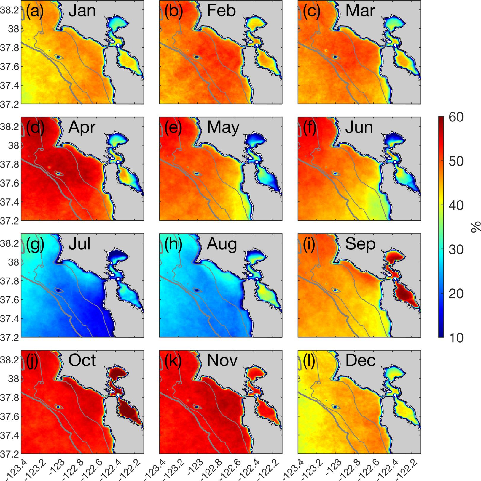
Figure 2. Percent of available observations for each month (a-l) from MODIS Aqua and Terra combined in the Gulf of Farallones region from 2002 to 2023. Availability of observations is influenced by cloud cover/marine layer contamination. Isobaths of 50, 100, and 200 are shown as gray contours, with a thicker contour denoting the 200 m isobath marking the shelf break.

2.3 Plume analysis

Turbid waters associated with the SFBP were identified and distinguished from adjacent ocean waters following the method first proposed by Nezlin and DiGiacomo (2005) and subsequently employed in a number of studies (e.g. Nezlin et al., 2005; Lahet and Stramski, 2010; Gonçalves et al., 2012). The method consists of finding a threshold value of radiance for plume boundary detection, with the threshold defined as the radiance value that maximizes the correlation between river discharge magnitude and the plume surface area. Threshold values of nLw555 from 0.5 to 2.0 mW cm^-2 µm^-1 sr^-1 were tested iteratively during clear sky days (data coverage above 95%), and weak wind conditions (along-shelf wind stress magnitude below the 25th percentile, 0.02 Pa) at different lags for river discharge and wind stress. A maximum correlation of 0.78 was found for a nLw555 level of 1.2 mW cm^-2 µm^-1 sr^-1, with a 5 day lag for discharge and a 1 day lag for along-shelf wind-forcing (Figure 3). The nLw555 level of 1.2 mW cm^-2 µm^-1 sr^-1 was therefore selected as the turbidity threshold for determining the presence of SFBP at each pixel for each day during the study period.

Figure 3

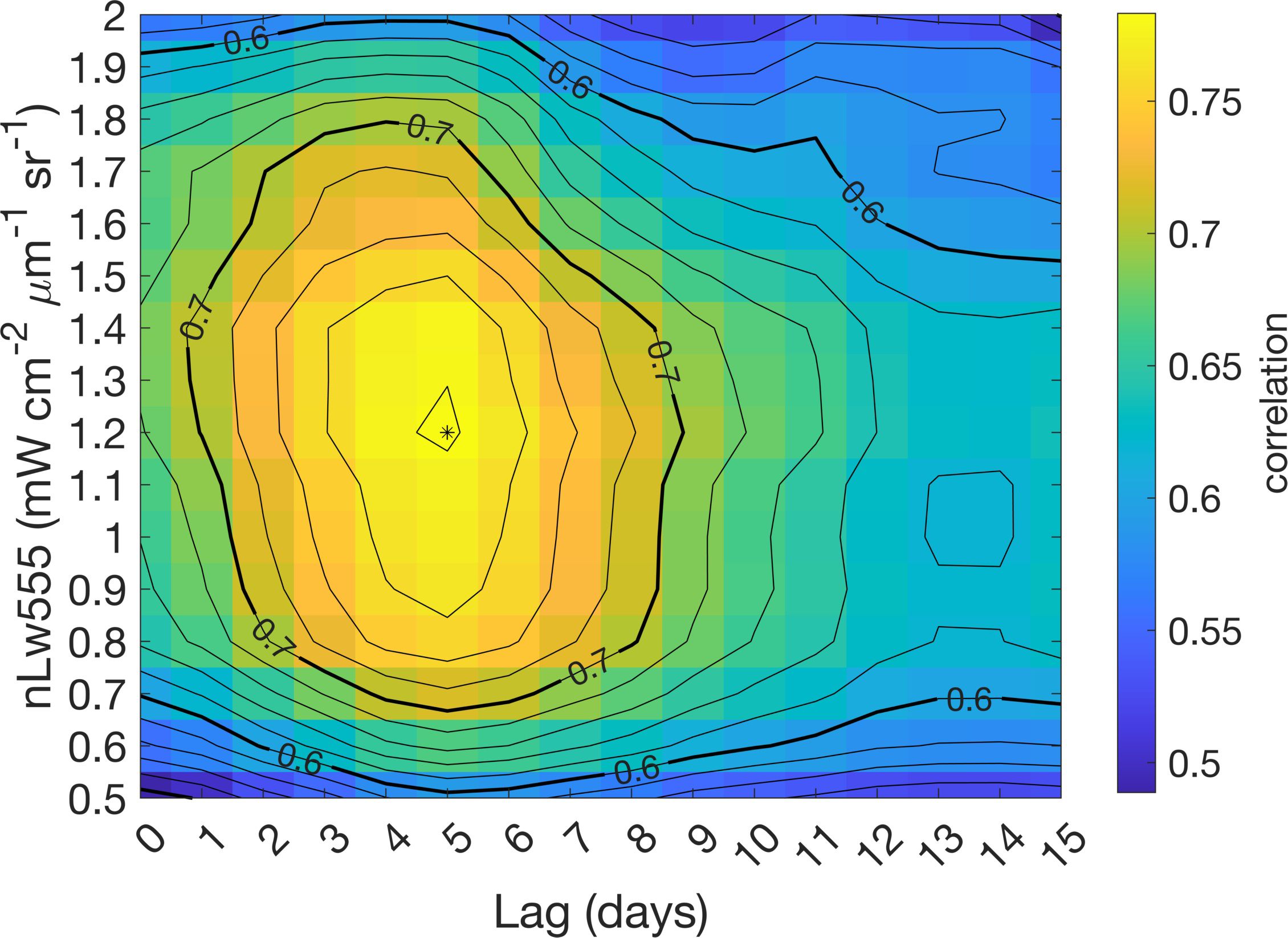
Figure 3. Correlation (shown in contours), between SFBP surface area bounded by different nLw555 levels and river discharge at different time lags, calculated during clear skies and weak wind conditions (with a 1-day lag to wind-forcing).

Frequency of plume occurrence was calculated monthly by dividing the number of times the SFBP was present at a given pixel (nLw555 levels greater than threshold of 1.2 mW cm^-2 µm^-1 sr^-1) by the number of days with available data in a given month (e.g., days with no clouds), and expressed in a percentage. All analyses conducted in this paper use the monthly frequency of plume occurrence, unless stated otherwise. The area of turbid SFBP influence in the GoF (which will be referred simply as “SFBP area”) was defined as the sum of the areas of all pixels, each weighted by the fraction of plume occurrence for each month; this calculation was conducted isolating the GoF region (bounded latitudinally between Pt Reyes and Pt Montara and offshore by the 200 m isobath), given the focus of this work, and to avoid the influence of smaller river outflows beyond the GoF limits (e.g. Speiser and Largier, 2024). Anomaly times series of plume area were then calculated by subtracting annual and semi-annual cycles computed through harmonic analysis (adding higher harmonics did not improve the skill of the fit), and were used to explore the potential relationship with forcings (winds, water level, discharge - see below).

At each pixel, frequency of SFBP occurrence was separated into intraseasonal, seasonal and interannual bands to quantify the relative contribution of these time scales to the overall plume variability (e.g. Martineac et al., 2024). This was done by first fitting annual and semi-annual cycles, and subtracting them from the frequency of plume occurrence time series. The resulting anomaly time series (original minus the annual and semi-annual cycles) was then high-pass filtered with an eight month cutoff to separate the intraseasonal band, and lowpass filtered with a sixteen month cutoff to separate the interannual band. Finally, the seasonal band was separated by band-passing the anomaly time series with cutoffs between eight and sixteen months, and adding back the fitted annual and semi-annual cycles. The error associated with this approximation (i.e., the difference between the variance of the original data and the sum of the variances from intraseasonal, seasonal and interannual time scales) was small, on average 8.2% (standard deviation: 2%).

3 Results

3.1 SFBP: mean characteristics

Average and standard deviation maps of SFBP frequency of occurrence, computed from monthly values for the entire study period (2002-2023), are shown in Figure 4. No measurable difference was noted between the values computed by averaging monthly frequency of occurrence as shown in Figure 4a from those calculated based on daily values from the entire time series (not shown). As expected, the average frequency of plume occurrence had maximum values (e.g. 100%) in the San Francisco Bay estuary, decaying radially exiting the Bay mouth, showing a coherent semi-circular plume shape. The SFBP edge is located between 10-20 km offshore around 50% of the time, reaching the 50 m isobath located 30 km offshore during 10% of the time. During extreme discharge cases, which occur less than 1% of the time, the plume extends to the shelf break, nearly 60 km offshore. The largest standard deviation values, 20-50%, can be seen between 10-30 km from Bay mouth, forming a band of radial shape. Standard deviation was also computed from a monthly climatology (not shown), and no measurable difference was noted from the calculation shown in Figure 4b. This demonstrates that tidal advection of the plume front is not the dominant signal in plume variability captured in our analysis. Instead, as it will be shown later, this variability is largely dominated by the seasonal cycle primarily due to varying river discharge.

Figure 4

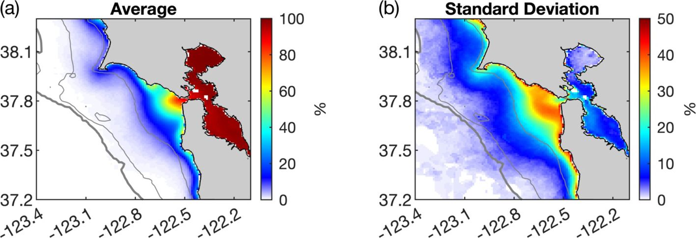
Figure 4. Maps showing the (a) average and (b) standard deviation of frequency of plume occurrence, calculated based on monthly values during the study period (2002-2023). Isobaths of 50, 100, and 200 m are shown as gray contours, with a thicker contour denoting the 200 m isobath marking the shelf break.

3.2 SFBP: mean response to wind-forcing and discharge

While gaps in the satellite record resulting from cloud cover contamination prevents resolving the plume at synoptic time scales (2-8 days), in order to inspect the average response of SFBP to a range of discharge and wind-forcing conditions, frequency of plume occurrences were created from daily images, selecting periods of low (below 150 m³/s, ~25^th percentile), moderate (between 150-500 m³/s, 25^th-75^th percentile), and high (above 500 m³/s, ~75^th percentile) discharge periods, as well as periods of moderate (magnitude<|0.04| Pa, median), upwelling-favorable (<-0.04 Pa, equatorward), and downwelling-favorable (>0.04 Pa, poleward) along-shelf winds. Frequency of plume occurrence was computed with daily images selected during periods combining the different discharge and wind conditions, taking into account 5 days lag for discharge and a 1 day lag for wind-forcing based on the maximum correlation with plume area (see Methods section, Figure 3), and results are shown in Figures 5a–i. During low discharge periods, the SFBP edge is located nearly 10 km offshore around 50% of the time, with no appreciable difference between moderate and upwelling-favorable winds. However, during low discharge periods with downwelling-favorable winds, a coastal current propagating poleward, separating from Pt. Reyes, and spreading and dispersing offshore, is observed (Figure 5d). As discharge intensifies, SFBP area notably increases, with the plume edge reaching 20-25 km offshore and just inshore of the 50 m isobath around 50% of the time. In extreme cases during high discharge, the plume extends all the way to the shelf break, located nearly 60 km offshore. Weak wind conditions show a quasi-symmetric radial plume spread from the Bay mouth, while during upwelling conditions the plume spreads southwestward, and during downwelling conditions an enhanced poleward coastal current is evident, with an associated eddy formed downstream of Pt. Reyes, with potentially significant retention of freshwater and associated substances and materials originating inside the Bay (Pareja-Roman et al., 2024).

Figure 5

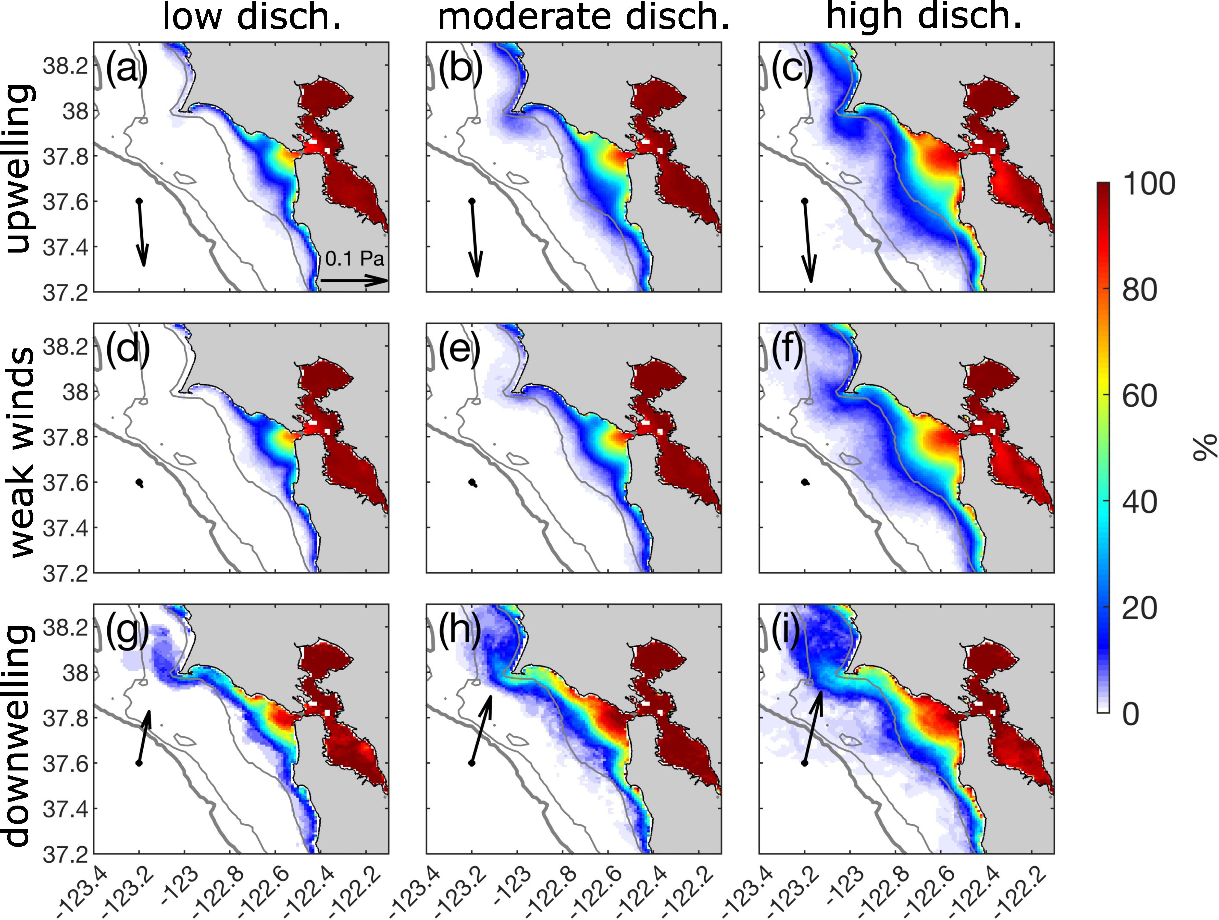
Figure 5. Maps showing frequency of plume occurrence for periods of (a, d, g) low (below 150 m³/s, ~25^th percentile), (b, e, h) moderate (between 150-500 m³/s, 25^th-75^th percentile), and (c, f, i) high (above 500 m³/s, ~75^th percentile) discharge, and periods of (a-c) upwelling-favorable (<-0.04 Pa), (d–f) moderate (magnitude<|0.04| Pa, median) and (g-i) downwelling-favorable (>0.04 Pa) winds. Shifts in 5 days were applied to discharge, and 1 day to wind-forcing based on the maximum correlation with plume area (see Methods section, Figure 3). Vectors on the left of each panel represent the average values of windstress calculated for each scenario. Isobaths of 50, 100, and 200 m are shown as gray contours, with a thicker contour denoting the 200 m isobath marking the shelf break.

3.3 SFBP: variability

Time series with monthly values of wind-forcing, water level, discharge, SFBP area, and frequency of plume occurrence as a function of offshore distance (along transect depicted in Figure 1), are shown in Figures 6a–e for the entire study period (2002-2023). A clear seasonal cycle can be seen in all variables, with noticeable interannual variability present particularly in water level and discharge. Along-shelf wind-forcing is on average upwelling-favorable, with reversals to downwelling-favorable during most winters and peaks varying nearly a factor of 2-3 from year to year. Annual peaks of discharge present a wide range of magnitudes, with over half of the years reaching above 1,000 m³/s, a quarter of the years above 2,000 m³/s, and during only three years of the record peaks were below 500 m³/s. Annual peaks of the SFBP area varied from 416 km³ to 1,894 km³, occupying 13% to 60% of the GoF area, respectively. A visual correspondence is apparent among discharge and plume area with large discharge peaks leading to notable increases in plume area (e.g. years 2006, 2017, 2019, 2023); in fact plume area and discharge are significantly correlated at the 95% confidence level and in phase (maximum correlation of 0.68 at zero month lag). The offshore extent of SFBP (along transect depicted in Figure 1) shows the edge of the turbid plume reaching nearly 30 km offshore around 50% of the time on most years, and in rare cases (<1% of the time) during extreme discharge levels, reaching the shelf break (2006, 2017).

Figure 6

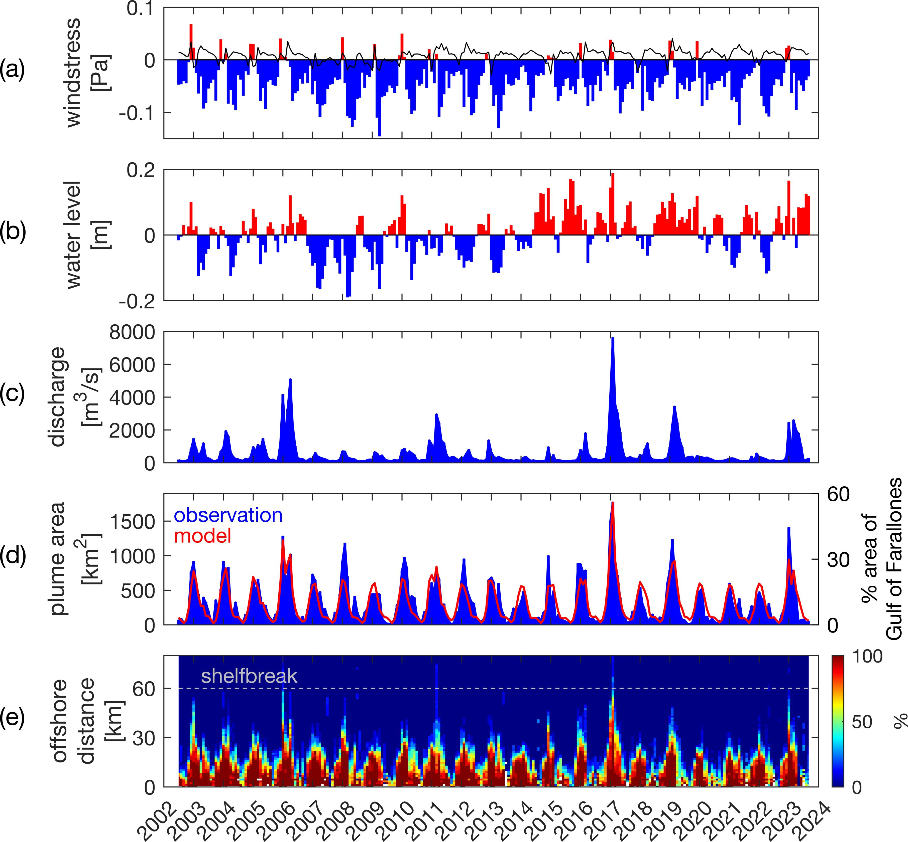
Figure 6. Time series with monthly values of (a) along- (blue and red bars) and cross-shelf (black line) windstress (b) water level, (c) river discharge, (d) SFBP area (left; blue: observations, red: regression model - Equations 1, 2) and percentage coverage of GoF (right), (e) Hovmöller diagram showing the frequency or plume occurrence as a function of time and offshore distance along the cross-shelf transect depicted in Figure 1.

To better visualize the seasonal cycle apparent in the time series (Figure 6), spatial maps of plume frequency of occurrence are shown in Figure 7 averaged for each month of the year, along with averaged monthly values of wind-forcing, water level, discharge, SFBP area, and frequency of plume occurrence as a function of offshore distance (along cross-shelf transect depicted in Figure 1) in Figure 8. SFBP area is smallest from mid-spring to fall (May-Nov), reaching a minimum in Aug-Sep, when the plume edge is located less than 10 km offshore around 50% of the time. These small plume areas of 27-28 km² (less than 1% of GoF area), coincide with low climatological discharge and weak, but sustained upwelling-favorable winds (“Relaxation Season”, García-Reyes and Largier, 2012). As discharge starts to increase in Dec and is sustained through the winter months, the SFBP area rapidly increases, reaching its largest value in Jan of ~700 km² (24% of GoF area), corresponding to when the plume edge is seen approximately 25-30 km offshore around 50% of the time. A steady decrease in plume area is then seen between late winter and mid-spring (Mar-May) even though the discharge only begins to decrease during spring (Apr-May). The mismatch between elevated discharge and plume area during those months could be attributed to the effect of winds: strengthening of upwelling-favorable winds during those months would lead to enhanced offshore Ekman transport that can thin out the plume and make it susceptible to mixing due to the vertically sheared horizontal currents (Fong and Geyer, 2001), consequently decreasing turbidity levels.

Figure 7

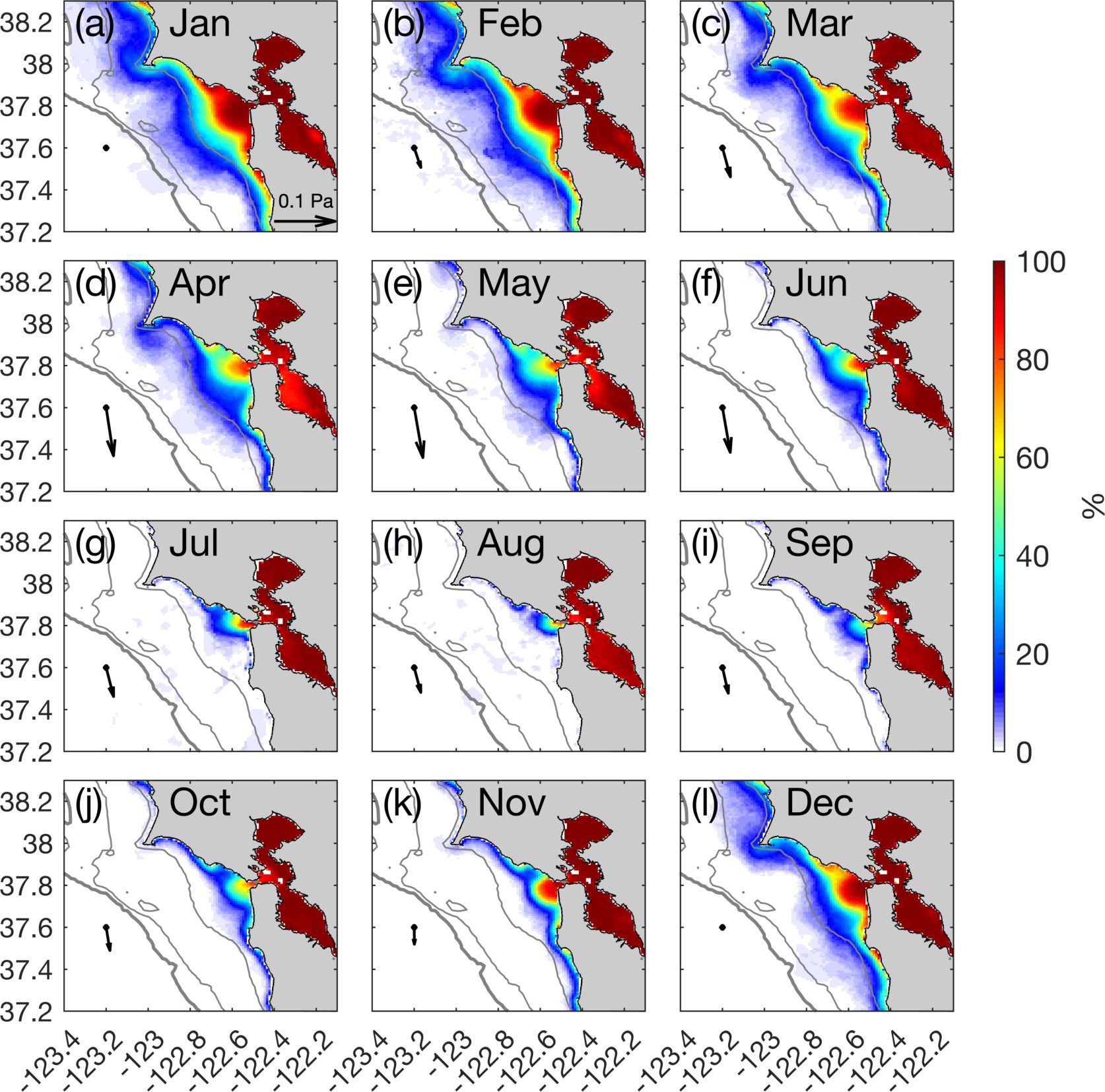
Figure 7. (a–l) Mean monthly frequency of occurrence of SFBP in the GoF. Vectors on the left of each panel represent the average values of windstress for each month. Isobaths of 50, 100, and 200 m are shown as gray contours, with a thicker contour denoting the 200 m isobath marking the shelf break.

Figure 8

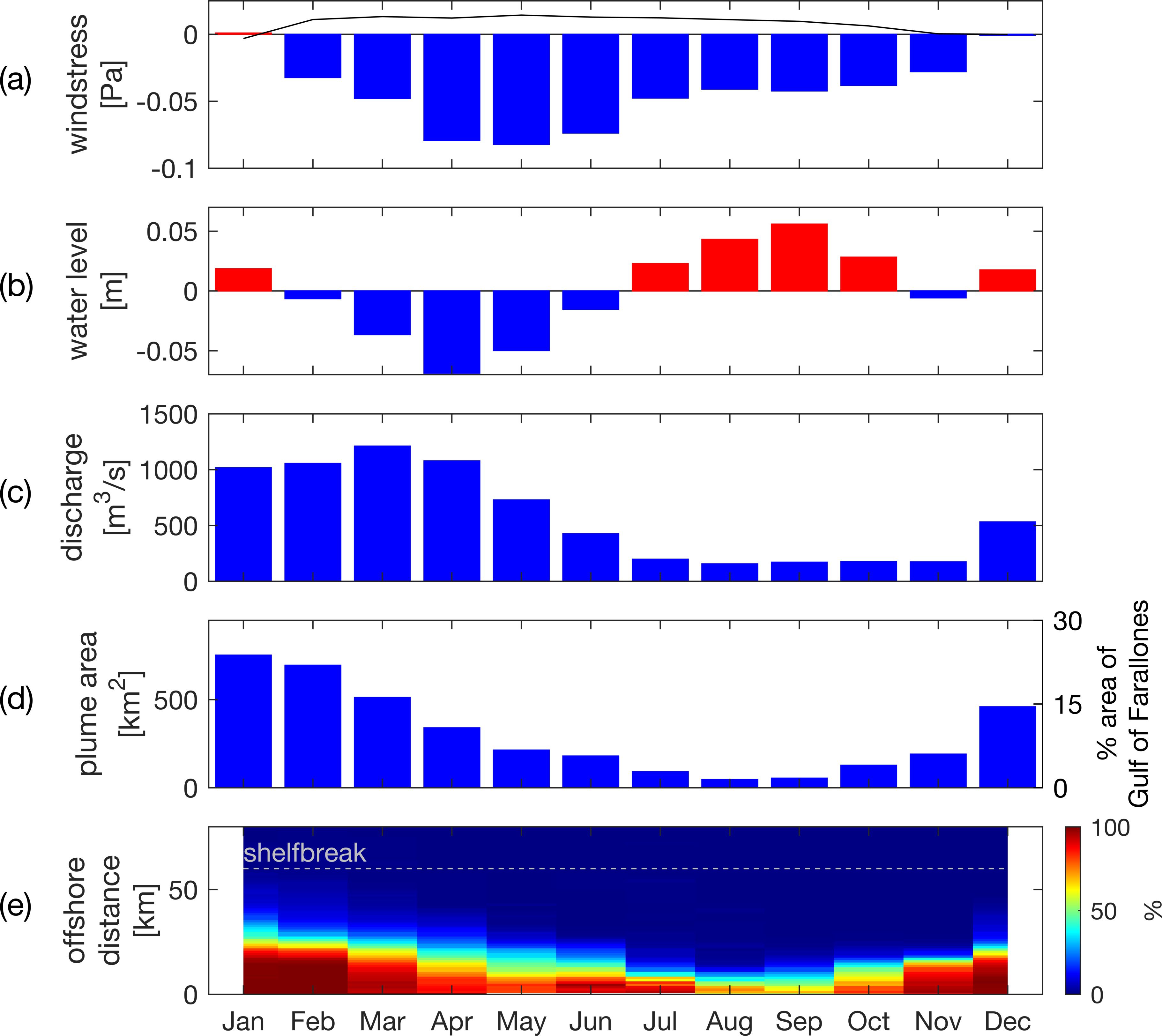
Figure 8. Seasonal cycle of (a) along- (blue and red bars) and cross-shelf (black line) windstress (b) water level, (c) river discharge, (d) SFBP area (left) and percentage coverage of GoF (right), (e) Hovmöller diagram showing frequency of plume occurrence as a function of time and offshore distance along the cross-shelf transect depicted in Figure 1.

Lastly, relative contributions of intraseasonal, seasonal and interannual time scales to the SFBP variability were computed at each pixel, shown in Figure 9. Inshore of the 50 m isobath, variability is largely dominated by the seasonal cycle, reaching up to 80% of the total variance, corresponding to the seasonal expansion-recession of the SFBP front shown in Figure 7 and coinciding with largest standard deviations shown in Figure 4. Offshore of the 50 m isobath, variability is dominated by intraseasonal band, explaining 50-80% of the total variance. Variability at those shorter time scales can be attributed to plume response to synoptic wind-forcing or due the filaments and eddies (e.g. Jia and Yankovsky, 2012). Finally, interannual variability contributed less than 20%, with greatest influence between the vicinity of the 50 m isobath and shelf break.

Figure 9

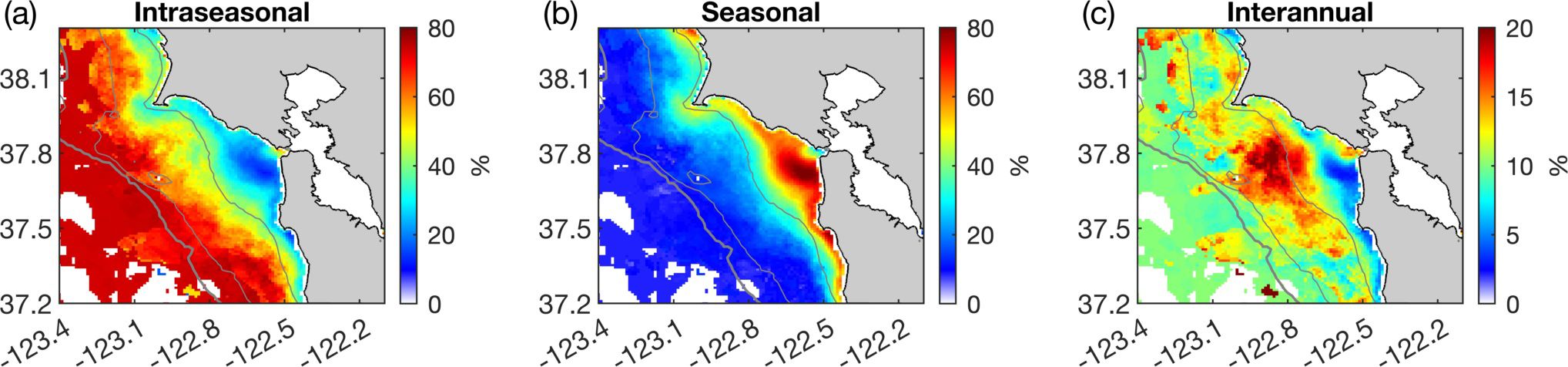
Figure 9. Percentage of total variance explained by (a) intraseasonal, (b) seasonal, and (c) interannual variability. Color scale on (c) is different to highlight spatial patterns. Pixels where SFBP is present less than 0.1% of the time are excluded. Isobaths of 50, 100, and 200 m are shown as gray contours, with a thicker contour denoting the 200 m isobath marking the shelf break.

3.4 Drivers of plume variability

To investigate the potential relationship between turbid SFBP and different forcings mechanisms at each pixel, cross-correlations were calculated between anomalies of frequency of SFBP occurrence against anomalies of discharge, along- and cross-shelf wind stress, and water level (proxy for pressure gradients), and are shown in Figure 10. Anomalies were chosen for this calculation since most variables are dominated by their respective seasonal cycles. The largest correlations, up to 0.8, are observed between SFBP and discharge, centered around the 50 m isobath offshore of the Bay mouth. Correlations between SFBP and other forcings, along- and cross-shelf winds and water level, are nearly half of those between SFBP and discharge (~0.4). Inshore of the 50 m isobath, negative correlations are observed between SFBP and along-shelf winds, which are typically thought as the major driver of plume frontal advection (e.g. Fong and Geyer, 2001; Moffat and Lentz, 2012; Pimenta and Kirwan, 2014, etc), and can be interpreted as classical Ekman response to wind-forcing: upwelling favorable winds (negative along-shelf values) advect the plume front offshore, increasing the occurrence in this area, while the opposite is true during downwelling-favorable winds (positive along-shelf values), hence the negative correlation. In the vicinity and offshore of the 50 m isobath, where correlations are positive, the plume is then presumably advected primarily by along-shelf currents, which follow wind-direction: for example, northward winds (positive along-shelf values) lead to an increase in plume presence in the central and northern parts of the GoF and north of Pt. Reyes (see Figure 5g-i), with southward winds having the opposite effect, hence the positive correlation values. The striking resemblance of correlations between SFBP and along-shelf wind-forcing with those between SFBP and other forcings (cross-shelf winds, water level) are likely due to the fact that all forcings are significantly correlated amongst themselves at the 95% confidence level (Table 1), and thus must be interpreted with caution. Cross-shelf winds are generally weak and unlikely to play an important role in the local plume dynamics in comparison with along-shelf wind-forcing. Moreover, the largest correlations among forcings were between water level and along-shelf wind-forcing, likely related to water level set up/set down in response to onshore/offshore Ekman transport. Due to the significant correlations amongst all forcings, it is not possible to disentangle their relative roles in the SFBP dynamics.

Figure 10

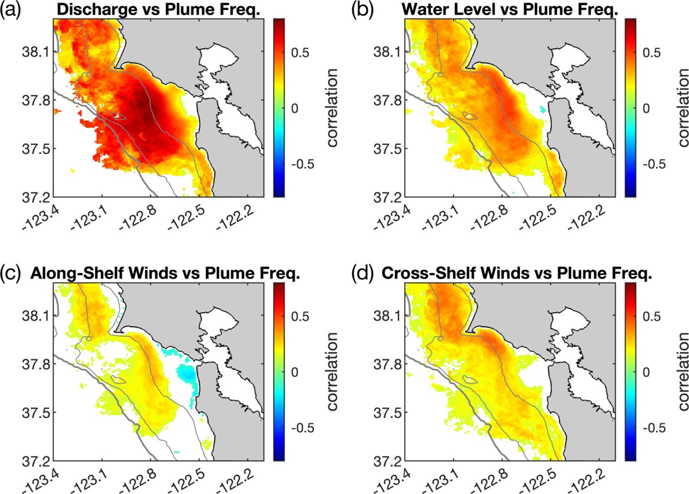
Figure 10. Cross-correlation between monthly anomalies (seasonal cycle removed) of frequency of SFBP occurrence and anomalies of (a) discharge, (b) water level, (c) along-shelf and (d) cross-shelf wind stress. Pixels where SFBP is present less than 0.1% of the time are excluded. Isobaths of 50, 100, and 200 m are shown as gray contours, with a thicker contour denoting the 200 m isobath marking the shelf break.

Table 1

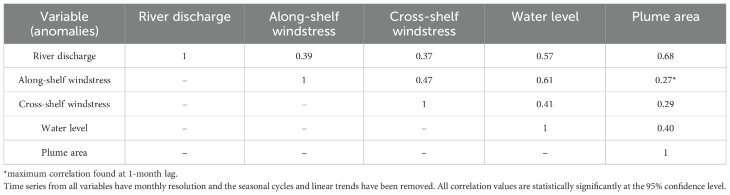
Table 1. Cross-correlation among the various forcings and SFBP area (determined by summing up all pixel areas weighted by their respective fraction of plume occurrence).

The cross-correlation between anomalies (seasonal cycles and linear trends removed) of forcings and the SFBP area are shown in Table 1. All forcings are significantly correlated with the SFBP at the 95% confidence level, with maximum cross-correlations at zero lag, with the exception of along-shelf wind-forcing, which had maximum correlations at one month lag. SFBP had the highest correlation with discharge (0.68), nearly twice the correlation with any other forcing. Next, a multivariable linear regression model that includes the annual and semi-annual cycles of plume area, and discharge, was created to explore the potential predictability of the SFBP area (SFBPArea_model, in km²) influencing the GoF region, and can be written as:

$\begin{array}{ll}SFBPAre{a}_{model}={\alpha }_0+{\alpha }_{1}sin(2\pi f_{1}t+{\phi }_1)+{\alpha }_{2}sin(2\pi f_{2}t+{\phi }_2)+{\alpha }_3{Q}_{anom}/\sigma (Q_{anom})& (1)\end{array}$

with

$\begin{array}{ll}{Q}_{anom}=Q-[{\beta }_0+{\beta }_{1}sin(2\pi f_{1}t+{\theta }_1)+{\beta }_{2}sin(2\pi f_{2}t+{\theta }_2)+{\beta }_{3}t]& (2)\end{array}$

where f₁ and f₂ are the annual and semi-annual frequencies, 1/365.25 and 2/365.25 days^-1 respectively, t is time in days, Q and Q_anom are the monthly discharge and discharge anomalies (m³/s), respectively, with σ representing standard deviation. Regression coefficient values obtained through least squared fitting are shown in Table 2. Discharge was normalized by its standard deviation so the magnitudes of regression coefficients α₁, α₂ and α₃ representing the relative importance of annual and semi-annual cycles of plume area and discharge, are all in km² and therefore could be directly compared. Given that all forcings are significantly correlated, only discharge was included in the model, since the inclusion of other forcings did not improve the skill of the model. Adding a long-term linear trend did not improve the skill of the model either, so it was omitted. Comparisons between SFBP area and model prediction according to Equations 1, 2 are shown in Figure 6d and Figure 11. Despite the simplicity of the model, it can explain over 78% of the total SFBP area variance at monthly time scales. Magnitudes of regression coefficients reveal that the annual cycle of plume area (α₁) has the largest amplitude, followed by the discharge and by the semi-annual cycle, which contribute to nearly 42% and 34% of the annual cycle amplitude, respectively.

Table 2

Table 2. Coefficients from multiple linear regression model, given by Equations 1, 2.

Figure 11

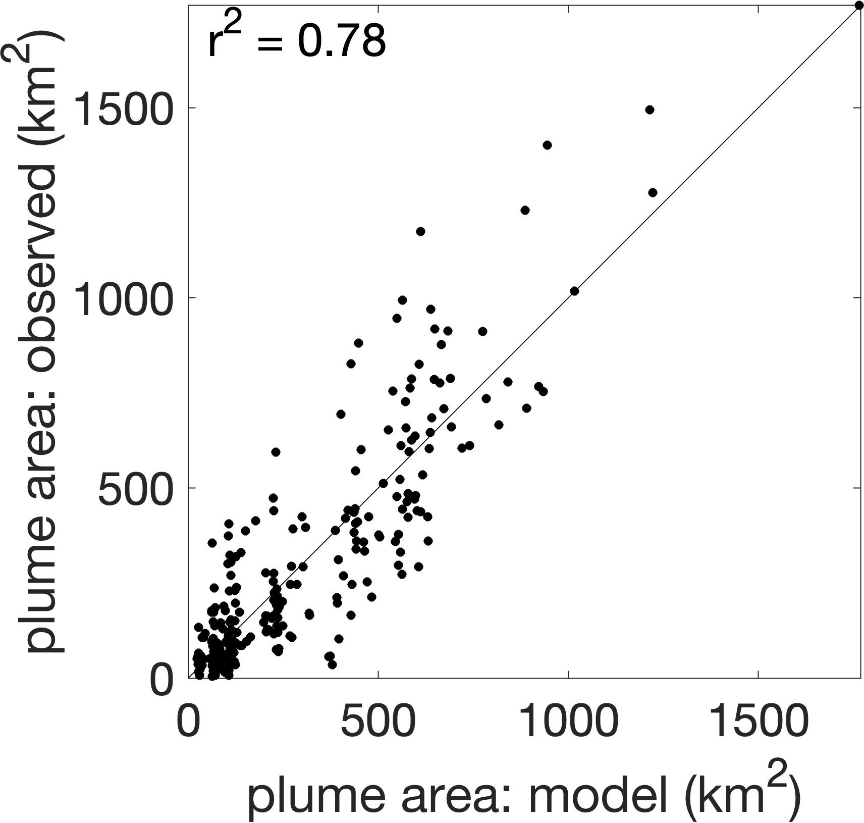
Figure 11. Comparison between observations of SFBP area and results from multiple linear regression model (Equation 1). Times series of model and observations are depicted in Figure 6d.

4 Discussion

This paper provides the first observationally based investigation of the spatio-temporal variability of the turbid SFBP from intraseasonal to interannual time scales, exploring 21 years (2002-2023) of ocean color data from MODIS and a plume tracking algorithm (Nezlin and DiGiacomo, 2005). Using the nLw555, which has been shown as reliable tracer of turbidity in the upper water column and used to study turbid river plumes throughout the world, including the U.S. West Coast from Oregon and Washington to southern California, we identified a turbidity threshold level of 1.2 mW cm^-2 µm^-1 sr^-1 (Figure 3) for determining the presence of SFBP turbid waters in the GoF. Analyzing monthly frequency of plume occurrence, we characterized the SFBP variability from intraseasonal to interannual time scales, assessed the influence of the plume in the GoF (quantifying the plume surface area), and investigated the relationship between the plume and main forcing mechanisms, including river discharge, winds and water level.

As the brackish and turbid San Francisco Bay waters exits the bay mouth, the plume spreads radially, and on average, it extends 10-20 km offshore, where the largest variability is also observed (Figure 4). However, during extreme discharge events, which occur less than 1% of the time, the turbid plume can reach all the way to the shelf break, located nearly 60 km offshore, constituting a direct pathway for exporting estuarine waters to the deep ocean. Our analysis revealed two distinct regions in which plume variability was controlled at different time scales and inherently associated processes. Inshore of the 50 m isobath (~30 km offshore of the Bay mouth), the seasonal cycle is dominant, explaining up to 80% of total variance, and plume variability is linked primarily to seasonal changes in river input. The largest plume areas were observed during winter months when discharge was enhanced, and the plume occupied up to 24% of the GoF area. In contrast, during summer months when discharge was minimal, plume occupied only 1.5% of GoF area. Offshore of the 50 m isobath, intraseasonal variability was dominant, explaining 50-80% of the total variance. Synoptic wind-forcing and mesoscale and submesoscale processes (e.g., filaments and eddies) are presumably dominant drivers of plume variability on these shorter time scales. Interannual variability plays a secondary role, explaining only 20% of total variance in this offshore region.

The mean plume response to river discharge and along-shelf wind-forcing was inspected by calculating frequency of plume occurrence during select forcing regimes, combining varying levels of discharge (low, moderate, high) and wind-forcing (upwelling, downwelling and weak winds) (Figure 5). For a given wind-forcing, as discharge increases, the plume area also increases, as typically expected. Plume response to wind-forcing follows classical Ekman dynamics, with upwelling-favorable winds advecting surface waters offshore through Ekman transport and therefore increasing plume area, and downwelling-favorable winds acting in the opposite sense, advecting surface waters in-shore, decreasing plume surface area (Lentz and Largier, 2006). In addition, during downwelling-favorable winds, an enhanced poleward propagating coastal current can be observed (Figures 5g-i), which diverts the brackish turbid waters to the north, minimizing the area of the plume’s bulge. As the coastal current passes through Pt. Reyes, it separates from the coast, and the formation of an eddy becomes evident (Pareja-Roman et al., 2024). Vander Woude et al. (2006) has shown that this is a retentive region with enhanced levels of chlorophyll, and our analysis suggests that the SFBP could play an important role in local biogeochemical cycling through the input of additional nutrients and/or the advection of phytoplankton from the estuary and GoF. These results provide evidence that the SFBP can influence regions beyond the GoF study area, and the remote influences of the plume should be pursued in future studies.

The primary productivity in the GoF, similar to the rest of the California Current System, is largely influenced by upwelling, which delivers nutrients from the subsurface waters into the euphotic zone. However, during periods of regional wind relaxation when the upwelling subsides, contrasting from most regions in the California Current System, the GoF has an additional source of nutrients and trace metals: the SFBP (Hurst and Bruland, 2008). The additional supply of nutrients from the SFBP is perhaps one of the reasons that makes the GoF one of the most productive regions in the California Current System (e.g. Wilkerson et al., 2006; Hurst and Bruland, 2008). The present study provides important insights into the spatial and temporal variability of the SFBP, and results could be used in conjunction with satellite remotely sensed chlorophyll and biogeochemical models to better understand the role of SFBP waters in the enhanced productivity in the GoF.

It is important to emphasize that this study relies on turbidity levels and not salinity to trace the SFBP, which likely provides a conservative estimate of the overall influence of San Francisco Bay waters in the GoF. Sediment aggregation and settling can reduce sediment concentrations within the plume, and therefore brackish waters can extend far beyond the optical signal studied here. A rare in situ surface salinity transect obtained by a Saildrone crossing the GoF during a high discharge event (2,350 m³ s^-1), shows a brackish plume with nearly constant salinity, of 27.5-29 PSU, extending 25 km offshore of the Golden Gate, which coincides with the edge of the turbid plume detected in this study during similar conditions (e.g. Figures 6c, e). Offshore, however, salinity increased nearly linearly and only reached a constant oceanic value (33.3 PSU) at the shelf break (Gentemann et al., 2020), which demonstrates that despite being diluted, San Francisco Bay waters influenced a much broader region. Furthermore, a recent numerical modeling study by Zhou et al. (2023), which investigated dispersal of the SFBP from 2011-2012, showed qualitatively similar seasonal behavior of the plume, with maximum extension during winter months and minimum during summer months, but the plume areas were biased high compared to the values obtained here. Unfortunately, quantitative estimates of plume area were not provided by the study for possible comparisons. Nevertheless, while the characterization of surface salinity remains out of the scope of this work, sustained in situ salinity measurements in the GoF region are crucial for making future progress in better understanding the dispersion of the SFBP. By combining in situ salinity observations with hyperspectral remotely sensed data from the newly launched Plankton, Aerosol, Cloud, ocean Ecosystem (PACE) satellite and leveraging machine learning techniques, high-resolution synthetic surface salinity maps could be generated for this region. This approach would provide a valuable data set for addressing the dispersion of SFBP and enhancing our understanding of its ecological impact in the GoF and beyond.

Finally, while all forcings analyzed here, including discharge, along- and cross-shelf winds and water level (proxy for pressure gradients) can impact the SFBP, it was not possible to disentangle their relative contributions to the plume’s variability, since all forcings were significantly correlated amongst themselves, even after removing their respective seasonal cycles and linear trends (Table 1). Discharge anomalies however had correlation values that were nearly double of any other forcing, and were therefore selected for constructing a predictive model of the SFBP area using multivariable linear regression (Equations 1, 2). In addition to discharge anomalies, the model included annual and semi-annual cycles of the plume area, and despite its simplicity, it explained over 78% of total variance of the turbid SFBP area, on monthly time scales. Linking discharge to the SFBP area in the GoF is particularly important since freshwater input from the Sacramento-San Joaquin Delta into the San Francisco Bay is highly managed to meet ecosystem objectives in the estuary by controlling the X₂: the 2 PSU bottom salinity isohaline intrusion distance (e.g. Monismith et al., 2002). The model developed here (Equations 1, 2) could be a useful tool for scientists and stakeholders to better understand how management actions on freshwater supply can have consequences offshore beyond the Golden Gate and help guide future management decisions in this ecologically important region.

Data availability statement

Publicly available datasets were analyzed in this study. This data can be found here: https://oceancolor.gsfc.nasa.gov/, https://data.cnra.ca.gov/dataset/dayflow, https://www.ndbc.noaa.gov/, https://tidesandcurrents.noaa.gov/.

Author contributions

PM: Conceptualization, Formal analysis, Investigation, Writing – original draft, Writing – review & editing. CP: Data curation, Methodology, Software, Writing – review & editing. FP: Writing – review & editing. KC: Writing – review & editing. RW: Writing – review & editing. RC: Writing – review & editing. EH: Writing – review & editing. RC: Writing – review & editing.

Funding

The author(s) declare that financial support was received for the research and/or publication of this article. We are grateful for funding provided by NOAA CA Sea Grant (Award NA18OAR4170073) and by the National Science Foundation (OCE award numbers 1948921, 1948675, 1948777).

Acknowledgments

We would like to thank the reviewers for their insightful suggestions. We are grateful for funding provided by NOAA CA Sea Grant (Award NA18OAR4170073) and by the National Science Foundation (OCE award numbers 1948921, 1948675, 1948777). MODIS images were made available by NASA Goddard Space Flight Center, Ocean Biology Processing Group. River discharge was provided by the California Department of Water Resources. Water level and wind speed and direction data were made available by NOAA.

Conflict of interest

The authors declare that the research was conducted in the absence of any commercial or financial relationships that could be construed as a potential conflict of interest.

Generative AI statement

The author(s) declare that no Generative AI was used in the creation of this manuscript.

Publisher’s note

All claims expressed in this article are solely those of the authors and do not necessarily represent those of their affiliated organizations, or those of the publisher, the editors and the reviewers. Any product that may be evaluated in this article, or claim that may be made by its manufacturer, is not guaranteed or endorsed by the publisher.

References

Bay Area Census (2025). Available online at: https://census.bayareametro.gov/ (Accessed June 9, 2025).

Google Scholar

Caballero I., Morris E. P., Pietro L., and Navarro G. (2014). The influence of the Guadalquivir river on spatio-temporal variability in the pelagic ecosystem of the eastern Gulf of Cádiz, Mediter. Mar. Sci. 15, 721–738. doi: 10.12681/mms.844

Crossref Full Text | Google Scholar

Caballero J. R. and Navarro G. (2011). Dynamics of the turbidity plume in the Guadalquivir estuary (SW Spain): A remote sensing approach (Santander, Spain: OCEANS 2011 IEEE - Spain), 1–11. doi: 10.1109/Oceans-Spain.2011.6003489

Crossref Full Text | Google Scholar

Carlson P. R. and McCulloch D. S. (1974). Aerial observations of suspended-sediment plumes in San Francisco Bay and the adjacent Pacific Ocean. J. Res. US Geol. Survey 2, 519–526.

Google Scholar

Castelao R. M. and Medeiros P. M. (2025). Satellite-derived dissolved organic carbon distribution and variability in an interconnected estuary off the Southeastern U.S. Estuar. Coasts 48, 12. doi: 10.1007/s12237-024-01455-3

Crossref Full Text | Google Scholar

Chant R. J., Wilkin J., Zhang W., Choi B., Hunter E., Castelao R., et al. (2008). Dispersal of the Hudson River plume in the New York Bight: Synthesis of observational and numerical studies during LaTTE. Oceanography 21, 148–161. doi: 10.5670/oceanog.2008.11

Crossref Full Text | Google Scholar

Conomos T. J. (1979). San Francisco Bay: The Urbanized Estuary (The Division, American Association for the Advancement of Science, Pacific Division, San Francisco), 493p.

Google Scholar

da Silva C. E. and Castelao R. M. (2018). Mississippi River plume variability in the Gulf of Mexico from SMAP and MODIS-Aqua observations. J. Geophys. Res.: Oceans 123, 6620–6638. doi: 10.1029/2018JC014159

Crossref Full Text | Google Scholar

Dykstra S. L., Ricche G., Marmorino G., and Yankovsky A. E. (2024). Forcing conditions of cross-shelf plumes on a wide continental shelf, Winyah Bay, South Atlantic Bight. Remote Sens. Environ. 311, 114279. doi: 10.1016/j.rse.2024.114279

Crossref Full Text | Google Scholar

Dzwonkowski B., Fournier S., Park K., Dykstra S. L., and Reager J. T. (2018). Water column stability and the role of velocity shear on a seasonally stratified shelf, Mississippi Bight, northern Gulf of Mexico. J. Geophys. Res.: Oceans 123, 5777–5796. doi: 10.1029/2017JC013624

Crossref Full Text | Google Scholar

Dzwonkowski B. and Yan X. H. (2005). Tracking of a Chesapeake Bay estuarine outflow plume with satellite-based ocean color data. Continent. Shelf Res. 25, 1942–1958. doi: 10.1016/j.csr.2005.06.011

Crossref Full Text | Google Scholar

Fisher A. W., Nidzieko N. J., Scully M. E., Chant R. J., Hunter E. J., and Mazzini P. L. F. (2018). Turbulent mixing in a far-field plume during the transition to upwelling conditions: Microstructure observations from an AUV. Geophys. Res. Lett. 45, 9765–9773. doi: 10.1029/2018GL078543

Crossref Full Text | Google Scholar

Fong D. A. and Geyer W. R. (2001). Response of a river plume during an upwelling favorable wind event. J. Geophys. Res. 106, 1067–1084. doi: 10.1029/2000jc900134

Crossref Full Text | Google Scholar

Fram J. P., Martin M. A., and Stacey M. T. (2007). Dispersive fluxes between the coastal ocean and a semienclosed estuarine basin. J. Phys. Oceanogr. 37, 1645–1660. doi: 10.1175/jpo3078.1

Crossref Full Text | Google Scholar

García-Reyes M. and Largier J. L. (2012). Seasonality of coastal upwelling off central and northern California: New insights, including temporal and spatial variability. J. Geophys. Res. 117, C03028. doi: 10.1029/2011JC007629

Crossref Full Text | Google Scholar

Gentemann C. L., Scott J. P., Mazzini P. L. F., Pianca C., Akella S., Minnett P. J., et al. (2020). Saildrone: adaptively sampling the marine environment. Bull. Amer. Meteor. Soc 101, E744–E762. doi: 10.1175/BAMS-D-19-0015.1

Crossref Full Text | Google Scholar

Gonçalves H., Teodoro A. C., and Almeida H. (2012). Identification, characterization and analysis of the Douro river plume from MERIS data. Appl. Earth Observ. Rem. Sens. 5, 1553–1563. doi: 10.1109/JSTARS.4609443

Crossref Full Text | Google Scholar

Gough M. K., Garfield N., and McPhee-Shaw E. (2010). An analysis of HF radar measured surface currents to determine tidal, wind-forced, and seasonal circulation in the Gulf of the Farallones, California, United States. J. Geophys. Res. 115, C04019. doi: 10.1029/2009JC005644

Crossref Full Text | Google Scholar

Hill A. E. (1998). “Buoyancy effects in coastal and shelf seas,” in The sea, vol. 11 . Eds. Robinson A. R. and Brink K. H. (John Wiley and Sons, Inc, Hoboken, New Jersey), 63–88.

Google Scholar

Holt B., Trinh R., and Gierach M. M. (2017). Stormwater runoff plumes in the Southern California Bight: a comparison study with SAR and MODIS imagery. Mar. pollut. Bull. 118, 141–154. doi: 10.1016/j.marpolbul.2017.02.040

PubMed Abstract | Crossref Full Text | Google Scholar

Horner-Devine A., Jay D., Orton P., and Spahn E. (2009). A conceptual model of the strongly tidal Columbia River plume. J. Mar. Syst. 78, 460–475. doi: 10.1016/j.jmarsys.2008.11.025

Crossref Full Text | Google Scholar

Hurst M. P. and Bruland K. W. (2008). The effects of the San Francisco Bay plume on trace metal and nutrient distributions in the Gulf of the Farallones. Geochim. Cosmochim. Acta 72, 395–411. doi: 10.1016/j.gca.2007.11.005

Crossref Full Text | Google Scholar

Jia Y. and Yankovsky A. E. (2012). The impact of ambient stratification on freshwater transport in a river plume. J. Mar. Res. 70, 69–92. doi: 10.1357/002224012800502408

Crossref Full Text | Google Scholar

Kakoulaki G., MacDonald D., and Horner-Devine A. R. (2014). The role of wind in the near field and midfield of a river plume. Geophys. Res. Lett. 41, 5132–5138. doi: 10.1002/2014GL060606

Crossref Full Text | Google Scholar

Kimmerer W. J. (2004). Open water processes of the San Francisco Estuary: from physical forcing to biological responses. San Francisco Estuar. Watershed Sci. 2, Article 1. Available online at: http://repositories.cdlib.org/jmie/sfews/vol2/iss1/art1 (Accessed July 22, 2025).

Google Scholar

Klemas V. (2012). Remote sensing of coastal plumes and ocean fronts: Overview and case study. J. Coast. Res. 28, 1–7. doi: 10.2112/JCOASTRES-D-11-00025.1

Crossref Full Text | Google Scholar

Lahet F., Ouillon S., and Forget P. (2001). Colour classification of coastal waters of the Ebro river plume from spectral reflectances. Int J Remote Sens 22, 1639–1664.

Google Scholar

Lahet F. and Stramski D. (2010). MODIS imagery of turbid plumes in San Diego coastal waters during rainstorm events. Remote Sens. Environ. 114, 332–344. doi: 10.1016/j.rse.2009.09.017

Crossref Full Text | Google Scholar

Large W. G. and Pond S. (1981). Open ocean momentum flux measurements in moderate to strong winds. J. Phys. Oceanogr. 11, 324–336. doi: 10.1175/1520-0485(1981)011<0324:OOMFMI>2.0.CO;2

Crossref Full Text | Google Scholar

Lemos A., Osadchiev A., Mazzini P. L. F., Mill G. N., Fonseca S. A. R., and Ghisolfi R. D. (2022). Spreading and accumulation of river-borne sedi-ments in the coastal ocean after the environmental disaster at the Doce River in Brazil. Ocean Coast. Res. 70, 1–18. doi: 10.1590/2675-2824070.21097atl

Crossref Full Text | Google Scholar

Lentz S. J. and Largier J. L. (2006). The influence of wind forcing on the Chesapeake Bay buoyant coastal current. J. Phys. Oceanogr. 36, 1305–1316. doi: 10.1175/JPO2909.1

Crossref Full Text | Google Scholar

Lihan T., Saitoh S. I., Iida T., Hirawake T., and Iida K. (2008). Satellite-measured temporal and spatial variability of the Tokachi River plume. Estuar. Coast. Shelf Sci. 78, 237–249. doi: 10.1016/j.ecss.2007.12.001

Crossref Full Text | Google Scholar

Lira J., Morales A., and Zamora F. (1997). Study of sediment distribution in the area of the Panuco river plume by means of remote sensing. Int. J. Remote Sens. 18, 171–182. doi: 10.1080/014311697219349

Crossref Full Text | Google Scholar

Loisel H., Bosc E., Stramski D., Oubelkheir K., and Deschamps P.-Y. (2001). Seasonal variability of the backscattering coefficient in the Mediterranean Sea based on satellite SeaWiFS imagery. Geophys. Res. Lett. 28, 4203–4206. doi: 10.1029/2001GL013863

Crossref Full Text | Google Scholar

MacDonald D. G., Goodman L., and Hetland R. D. (2007). Turbulent dissipation in a near-field river plume: A comparison of control volume and microstructure observations with a numerical model. J. Geophys. Res. 112, C07026. doi: 10.1029/2006JC004075

Crossref Full Text | Google Scholar

Martineac R. P., Castelao R. M., and Medeiros P. M. (2024). Seasonal and interannual variability in the distribution and removal of terrigenous dissolved organic carbon in the Amazon River plume. Global Biogeochem. Cycles 38, e2023GB007995. doi: 10.1029/2023GB007995

Crossref Full Text | Google Scholar

Mazzini P. L. F., Barth J. A., Shearman R. K., and Erofeev A. (2014). Buoyancy-driven coastal currents off Oregon during Fall and Winter. J. Phys. Oceanogr. 44, 2854–2876. doi: 10.1175/JPO-D-14-0012.1

Crossref Full Text | Google Scholar

Mazzini P. L. F. and Chant R. J. (2016). Two-dimensional circulation and mixing in the far field of a surface-advected river plume. J. Geophys. Res.: Oceans 121, 3757–3776. doi: 10.1002/2015JC011059

Crossref Full Text | Google Scholar

Mazzini P. L. F., Chant R. J., Scully M. E., Wilkin J., Hunter E. J., and Nidzieko N. J. (2019). The impact of wind forcing on the thermal wind shear of a river plume. J. Geophys. Res.: Oceans 124, 7908–7925. doi: 10.1029/2019JC015259

Crossref Full Text | Google Scholar

Mazzini P. L. F., Risien C. M., Barth J. A., Pierce S., Erofeev A., Dever E., et al. (2015). Anomalous near-surface low-salinity pulses off the central Oregon coast. Sci. Rep. 5, (17145). doi: 10.1038/srep17145

PubMed Abstract | Crossref Full Text | Google Scholar

Mendes R., Vaz N., Fernández-Nóvoa D., da Silva J. C. B., de Castro M., Gómez-Gesteira M., et al. (2014). Observation of a turbid plume using MODIS imagery: the case of Douro estuary (Portugal). Remote Sens. Environ. 154, 127–138. doi: 10.1016/j.rse.2014.08.003

Crossref Full Text | Google Scholar

Moffat C. and Lentz S. J. (2012). On the response of a buoyant plume to downwelling-favorable wind stress. J. Geophys. Res. 42, 1083–1098. doi: 10.1175/JPO-D-11-015.1

Crossref Full Text | Google Scholar

Monismith S. G., Kimmerer W., Burau J. R., and Stacey M. T. (2002). Structure and flow-induced variability of the subtidal salinity field in northern San Francisco Bay. J. Phys. Oceanogr. 32, 3003–3019. doi: 10.1175/1520-0485(2002)032<3003:SAFIVO>2.0.CO;2

Crossref Full Text | Google Scholar

Nash J. D. and Moum J. N. (2005). River plumes as a source of large-amplitude internal waves in the coastal ocean. Nature 437, 400–403. doi: 10.1038/nature03936

PubMed Abstract | Crossref Full Text | Google Scholar

Nezlin N. P. and DiGiacomo P. M. (2005). Satellite ocean color observations of stormwater runoff plumes along the San Pedro Shelf (southern California) during 1997-2003. Continent. Shelf Res. 25, 1692–1711. doi: 10.1016/j.csr.2005.05.001

Crossref Full Text | Google Scholar

Nezlin N. P., DiGiacomo P. M., Stein E. D., and Ackerman D. (2005). Stormwater runoff plumes observed by SeaWiFS radiometer in the Southern California Bight. Remote Sens. Environ. 98, 494–510.

Google Scholar

Nezlin N. P., DiGiacomo P. M., Diehl D. W., Jones B. H., Johnson S. C., Mengel M. J., et al. (2008). Stormwater plume detection by MODIS imagery in the southern California coastal ocean. Estuar. Coast. Shelf Sci. 80, 141–152. doi: 10.1016/j.ecss.2008.07.012

Crossref Full Text | Google Scholar

Otero M. P. and Siegel D. A. (2004). Spatial and temporal characteristics of sediment plumes and phytoplankton blooms in the Santa Barbara Channel. Deep Sea Res. II 51, 1129–1149. doi: 10.1016/S0967-0645(04)00104-3

Crossref Full Text | Google Scholar

Palacios S. L., Peterson T. D., and Kudela R. M. (2009). Development of synthetic salinity from remote sensing for the Columbia River plume. J. Geophys. Res. 114, C00B05. doi: 10.1029/2008JC004895

Crossref Full Text | Google Scholar

Pareja-Roman L. F., Chant R. J., Mazzini P. L. F., and Cole K. (2024). Circulation and retention of river plumes around capes. J. Geophys. Res.: Oceans 129, e2023JC020645. doi: 10.1029/2023JC020645

Crossref Full Text | Google Scholar

Pimenta F. M. and Kirwan A. D. Jr. (2014). The response of large outflows to wind forcing. Continent. Shelf Res. 89, 24–37. doi: 10.1016/j.csr.2013.11.006

Crossref Full Text | Google Scholar

Pimenta F. M., Kirwan J. A. D., and Huq P. (2011). On the transport of buoyant coastal plumes. J. Phys. Oceanogr. 41, 620–640. doi: 10.1175/2010JPO4473.1

Crossref Full Text | Google Scholar

Saldias G. S., Shearman R. K., Barth J. A., and Tufillaro N. (2016). Optics of the offshore Columbia River plume from glider observations and satellite imagery. J. Geophys. Res. Oceans 121, 2367–2384. doi: 10.1002/2015JC011431

Crossref Full Text | Google Scholar

Saldias G. S., Sobarzo M., Largier J., Moffat C., and Letelier R. (2012). Seasonal variability of turbid river plumes off central Chile based on high-resolution MODIS imagery. Remote Sens. Environ. 123, 220–233. doi: 10.1016/j.rse.2012.03.010

Crossref Full Text | Google Scholar

Schofield O., Arnone R. A., Bissett W. P., Dickey T. D., Davis C. O., Finkel Z., et al. (2004). Watercolors in the coastal zone: What can we see? Oceanography 17, 24–31. doi: 10.5670/oceanog.2004.44

Crossref Full Text | Google Scholar

Shi W. and Wang M. (2007). Detection of turbid waters and absorbing aerosols for the MODIS ocean color data processing. Remote Sens. Environ. 110, 149–161. doi: 10.1016/j.rse.2007.02.013

Crossref Full Text | Google Scholar

Shi W. and Wang M. (2010). Satellite observations of the seasonal sediment plume in central East China Sea. J. Mar. Syst. 82, 280–285. doi: 10.1016/j.jmarsys.2010.06.002

Crossref Full Text | Google Scholar

Speiser W. H. and Largier J. L. (2024). Long-term observations of the turbid outflow plume from the Russian River, California. Estuar. Coast. Shelf Sci. 309, 108942. doi: 10.1016/j.ecss.2024.108942

Crossref Full Text | Google Scholar

Steger J. M., Schwing F. B., Collins C. A., Rosenfeld L. K., Garfield N., and Gezgin E. (2000). The circulation and water masses in the Gulf of the Farallones. Deep Sea Res. Part II 47, 907–946. doi: 10.1016/S0967-0645(99)00131-9

Crossref Full Text | Google Scholar

Thomas A. C. and Weatherbee R. A. (2006). Satellite-measured temporal variability of the Columbia River plume. Remote Sens. Environ. 100, 167–178. doi: 10.1016/j.rse.2005.10.018

Crossref Full Text | Google Scholar

Toole D. A. and Siegel D. A. (2001). Modes and mechanisms of ocean color variability in the Santa Barbara Channel. J. Geophys. Res. Oceans 106, 26985–27000. doi: 10.1029/2000JC000371

Crossref Full Text | Google Scholar

Vander Woude A. J., Largier J. L., and Kudela R. M. (2006). Nearshore retention of upwelled waters north and south of Point Reyes (northern California)Patterns of surface temperature and chlorophyll observed in CoOp WEST. Deep Sea Res. Part II 53, 2985–2998. doi: 10.1016/j.dsr2.2006.07.003

Crossref Full Text | Google Scholar

Wall C. C., Muller-Karger F. E., Roffer M. A., Hu C., Yao W., and Luther M. E. (2008). Satellite remote sensing of surface oceanic fronts in coastal waters off west-central Florida. Remote Sens. Environ. 112, 2963–2976. doi: 10.1016/j.rse.2008.02.007

Crossref Full Text | Google Scholar

Walters R. A., Cheng R. T., and Conomos T. J. (1985). Time scales of circulation and mixing processes of San Francisco Bay waters. Hydrobiologia 129, 13–37. doi: 10.1007/BF00048685

Crossref Full Text | Google Scholar

Wang Y.-H., Ruttenberg B. I., Walter R. K., Pendleton F., Samhouri J. F., Liu O. R., et al. (2024). High resolution assessment of commercial fisheries activity along the US West Coast using Vessel Monitoring System data with a case study using California groundfish fisheries. PloS One 19, e0298868. doi: 10.1371/journal.pone.0298868

PubMed Abstract | Crossref Full Text | Google Scholar

Wang M. and Shi W. (2007). The NIR-SWIR combined atmospheric correction approach for MODIS ocean color data processing. Optics Express 15, 15722. doi: 10.1364/OE.15.015722

PubMed Abstract | Crossref Full Text | Google Scholar

Wang M., Son S., and Shi W. (2009). Evaluation of MODIS SWIR and NIR-SWIR atmospheric correction algorithms using SeaBASS data. Remote Sens. Environ. 113, 635–644. doi: 10.1016/j.rse.2008.11.005

Crossref Full Text | Google Scholar

Warrick J. A., Mertes L. A. K., Washburn L., and Siegel D. A. (2004). Dispersal forcing of southern California river plumes, based on field and remote sensing observations. Geo Marine Lett. 24, 46–52. doi: 10.1007/s00367-003-0163-9

Crossref Full Text | Google Scholar

Wilkerson F. P., Lassiter A., Dugdale R. C., Marchi A., and Hogue V. (2006). The phytoplankton bloom response to wind events and upwelled nutrients during the CoOP WEST study. Deep Sea Res. 53, 3023–3048. doi: 10.1016/j.dsr2.2006.07.007

Crossref Full Text | Google Scholar

Yankovsky A. E. (2006). On the validity of thermal wind balance in along shelf currents off the New Jersey coast. Continent. Shelf Res. 26, 1171–1183. doi: 10.1016/j.csr.2006.03.008

Crossref Full Text | Google Scholar

Yankovsky A. E. and Voulgaris G. (2019). Response of a coastal plume formed by tidally-modulated estuarine outflow to light upwelling-favorable wind. J. Phys. Oceanogr. 49, 691–703. doi: 10.1175/jpo-d-18-0126.1

Crossref Full Text | Google Scholar

Zhou J., Izett J. G., Edwards C. A., Damien P., Kessouri F., and McWilliams J. C. (2023). Modeling the dispersal of the San Francisco Bay plume over the northern and central California shelf. Estuar. Coast. Shelf Sci. 287, 108336. doi: 10.1016/j.ecss.2023.108336

Crossref Full Text | Google Scholar