Abstract
Predation and secondary foundation species play crucial roles in structuring sessile mangrove prop root communities. However, their relative importance and their interactions across biogeographic gradients remain poorly understood. This study investigated the impact of predation and secondary foundation species on mangrove prop root epibiont assemblages along a latitudinal gradient in Florida. Predator exclusion treatments were deployed at four sites spanning tropical to temperate zones, and community development was monitored over 6 months. The results showed that the effects of predation shifted with latitude, from increasing the species richness in the south while reducing it in the north. Secondary foundation species, such as sponges, oysters, and barnacles, generally outcompeted other species for space in the early colonization stages, but tended to increase biodiversity when space was not limiting. Secondary foundation species also exhibited context-dependent associations with species richness across the latitudinal gradient. Sponges and oysters tended to enhance the species richness under reduced predation pressure, while barnacles generally had negative effects at higher latitudes. The multivariate analyses revealed that the interaction between predation and latitude explained more variation in the community structure than predation alone, and secondary foundation species contributed significantly to these patterns. The findings support the predation hypothesis and facilitation by secondary foundation species in shaping mangrove prop root community shifts across biogeographic gradients, providing insights into the complex interactions structuring mangrove epibiont communities.
Introduction
The principal questions in community ecology are: how are communities structured; what mechanisms direct this structure; and do these mechanisms change over spatial, temporal, or abiotic gradients. The species diversity within ecological communities greatly influences the functioning of an ecosystem (Edwards et al., 2010; Belley and Snelgrove, 2016; Brisson et al., 2020). Understanding the direction and strength of the drivers of these observed ecological patterns is especially important as it pertains to predicted climatic changes. Ecological community patterns are enmeshed in the interplay between abiotic factors and interspecies interactions, and untangling this labyrinth of linkages is essential to unlocking the latitudinal gradient first described by Darwin and Wallace (Darwin, 1859; Darwin and Wallace, 1958; Wallace, 1905; Willig et al., 2003; Scheiner and Willig, 2005). With so many factors influencing ecological communities, assessing which of these factors have large effects on community structure is at the core of modeling and understanding ecosystems.
One general pattern of ecological biodiversity is that of higher biodiversity in tropical latitudes and declining biodiversity with increasing latitude (Hillebrand, 2004; Yasuhara et al., 2012; Parravicini et al., 2013; Tittensor et al., 2010). One hypothesis explaining the latitudinal gradient is the species richness–energy hypothesis, which states that there is more energy—in the form of solar radiation—near the equator. Moreover, this has been proven to be a good measure of biodiversity along the latitudinal gradient. Central to this hypothesis is the biological fact that biochemical activities, in general, increase with increased temperature (Aquino, 1968), which results in a faster rate of evolutionary change, resulting in higher biodiversity (Rohde, 1992; Taylor and Gaines, 1999; Willig et al., 2003; Mittelbach et al., 2007; Tittensor et al., 2010). This hypothesis has been supported by many studies (Macpherson, 2002), in which the mean annual temperature has been proven to be a good measure of energy in the system.
Predation has been put forth as another of the driving forces of trait divergence in the biotic interaction hypothesis (Pianka, 1966; Rohde, 1992). The biotic interaction hypothesis states that, in the tropics, species interactions are stronger and comprise a greater portion of evolutionary selection, which results in traits evolving faster (Willig et al., 2003; Mittelbach et al., 2007; Brown, 2014). Of the interactions that help explain community development, a number of studies have assessed the effects of predation across a latitudinal gradient (Reynolds et al., 2018). Top-down pressure from predation has a strong influence on the community structure, especially in marine environments (Edwards et al., 2010; Sheppard-Brennand et al., 2017; Reynolds et al., 2018).
Current ecological theory states that predation decreases with increasing latitude (Sheppard-Brennand et al., 2017). Predation pressure affecting community diversity differently across a latitudinal gradient has been recorded in shallow water systems worldwide (Pianka, 1966; Freestone et al., 2011; Sheppard-Brennand et al., 2017). The marine benthic community is structured by two important biological processes: colonization by larvae (Schwamborn and Bonecker, 1996; Leal et al., 2019; Rossi et al., 2018) and post-settlement survival (Thorson, 1966; Sutherland, 1974; Osman and Whitlatch, 1995; Freestone et al., 2011; Yakovis and Artemieva, 2017). Predation plays a prominent role in post-settlement survival (Gosselin and Qian, 1997; Kulp and Peterson, 2016). The predation hypothesis states that predation pressure lowers the level of competition, thus allowing for higher biodiversity through the coexistence of more prey species (Pianka, 1966).
Another strong influence of community structure is the bottom-up impact of foundation species (Cusseddu et al., 2016; Sala et al., 2008). As the old adage in architecture states, “structure dictates function.” The organization of an ecosystem is based on the structure of the foundation species as this dictates diversity, resilience, food web complexity, and productivity (Dayton, 1972; Bruno and Bertness, 2001; Yakovis and Artemieva, 2017). The interactions between co-occurring foundation species can have significant influences on predator–prey interactions (Ware et al., 2019), the trophic structure, and other ecological functions (Altieri et al., 2007; Angelini and Silliman, 2014; Yakovis and Artemieva, 2017). Much of the ecological effects of foundation species are due to their habitat-modifying capabilities (O'Brien et al., 2018; Vozzo and Bishop, 2019; Yakovis and Artemieva, 2019). The interstitial spatial structure of foundation species affects predator–prey interactions (Ware et al., 2019). In Florida’s mangrove, ecosystem shifts in the secondary foundation species—foundation species that reside on mangrove prop roots—had a strong influence on the epifaunal biodiversity on mangrove prop roots (Aquino-Thomas and Proffitt, 2025).
Red mangroves are a foundation species and ecological engineer that influences the microclimate, sedimentation, and subsidence rates and provides many ecological functions and services (Feller et al., 2010; Aquino-Thomas and Proffitt, 2014; Doughty et al., 2016; Aquino-Thomas, 2020). Collectively, mangrove species will be referred to here as the primary foundation species. Encrusting communities of invertebrates and algae form on the prop roots of red mangroves and can serve as secondary foundation species by influencing the diversity of many small motile and sessile species. By modifying the physical environment of the communities, these species create microhabitats with varying levels of light, water flow, and nutrient availability (Bishop et al., 2012; Angelini and Silliman, 2014; Thomsen et al., 2018; Ellison, 2019). This heterogeneity supports a greater variety of other organisms, including filter feeders, photosynthetic species, and detritivores (Sebens, 1991; Gallucci et al., 2020; Thomsen et al., 2022). This combination of foundation species, and the associated community, provides a unique opportunity to assess the effects of predation in a two-foundation species system along an environmental gradient. The space-for-time substitution (Pickett, 1989) along the latitudinal gradient will affect the dominance of the foundation species (Aquino-Thomas and Proffitt, 2025) and the influence of predators, which may vary with the differences in interstitial spaces that occur with different dominant taxa comprising the secondary foundation species. The supplemental refuge effects of having multiple foundation species is greatly influenced by the extent of the functional redundancy between foundation species (Vozzo and Bishop, 2019). This feature of foundation species creating refuge from predation has been shown to be important in varied ecosystems, such as mobile sea urchins (Altieri and Witman, 2014), Australian mangroves (Vozzo and Bishop, 2019), macroalgal ecosystems (O'Brien et al., 2018; Ware et al., 2019), red mangroves (Schutte and Byers, 2017), kelp forests (Efird and Konar, 2014), coral reefs (Dunn et al., 2017), oyster reefs (McAfee and Bishop, 2019), and even dead oysters (Tomatsuri and Kon, 2017).
Predation and secondary foundation species play crucial roles in structuring sessile mangrove prop root communities. However, their relative importance and their interactions across biogeographic gradients remain poorly understood. While previous studies have examined predation effects or foundation species’ impacts individually, only a few have investigated how these factors interact across large spatial scales to shape community assembly. This study aimed to fill this knowledge gap by assessing the combined effects of predation and secondary foundation species on mangrove epibiont communities along a latitudinal gradient in Florida.
The overall objective of this field experiment was to assess the relative influence of predation and secondary foundation species on the mangrove prop root species diversity along the latitudinal gradient. By deploying predator exclusion treatments at four sites spanning from tropical to temperate zones and by monitoring community development over 6 months, we aimed to elucidate how top-down and bottom-up forces interact to structure these communities across biogeographic regions. We hypothesize that: a) the effects of predation on community structure will shift from positive in tropical sites to negative in temperate sites, in line with the predation hypothesis; b) secondary foundation species will generally increase biodiversity when space is not limiting, but their effects will vary depending on the predation pressure and latitude; c) the interaction between predation and secondary foundation species will explain more variation in the community structure than either factor alone; and d) the relative importance of predation versus facilitation by secondary foundation species in shaping communities will shift across the latitudinal gradient.
Methods
Field experiment design
The field experiment was conducted between June and December 2015 and used a method similar to that in Freestone et al. (2011). Sessile species are easily tracked and have relatively fast growth rates, making them particularly suitable for use in ecological studies (Freestone et al., 2013). The latitudinal gradient was separated into four zones. The four zones were established by the identity of the species present (Aquino-Thomas and Proffitt, 2025), and one site from each zone was selected for the field experiment. The sites (a fixed factorial variable) selected for use in the experiment were located toward the center of a zone (which was not possible in Miami–Dade as access to large mangrove stands was restricted) and were dominated by red mangrove (Rhizophora mangle) trees situated in water with salinity typically ranging between 32 and 35 psu. The study covered 380 km from the Florida Keys to Fort Pierce, Florida. For estuarine macroinvertebrate communities, Palm Beach County is a tropical-to-temperate biogeographic change point (Engle and Summers, 1999). Research has found a distinct change in the benthic community composition between latitudes of 25° and 27° (Engle and Summers, 1999; Walker, 2012).
The experiment was conducted concurrently at four mangrove sites in South Florida: Curry Hammock (24°44′40.1′′), Arch Creek (25°54′06.2′′), James Rutherford (26°21′54.2′′), and Harbor Branch Oceanographic Institute (HBOI) (27°32′13.2′′) (Figure 1). Environmental data were recorded from these sites three times, although data from the Arch Creek site at time 2 were lost due to equipment failure. Curry Hammock had low colonization, and due to inclement weather and the travel distance, it was decided that the planned second revisit could be eliminated. The site characteristics included in the experimental analysis were the following: distance from the inlet, distance from freshwater discharge, distance to the mangrove stand to the north, distance to the mangrove stand to the south, mangrove km (the total distance, north and south, that the fringe mangrove shoreline extended from the sampled tree), sediment type (the ranked sedimentation size from shell to silt/mud), mangrove connectivity (the percentage of fringe mangrove shoreline 1 km north and south of the sample), the longest fetch, the shortest fetch, and latitude. Human disturbance impacts were measured by the distance to the nearest boat lanes and the distance to the docks.
Figure 1
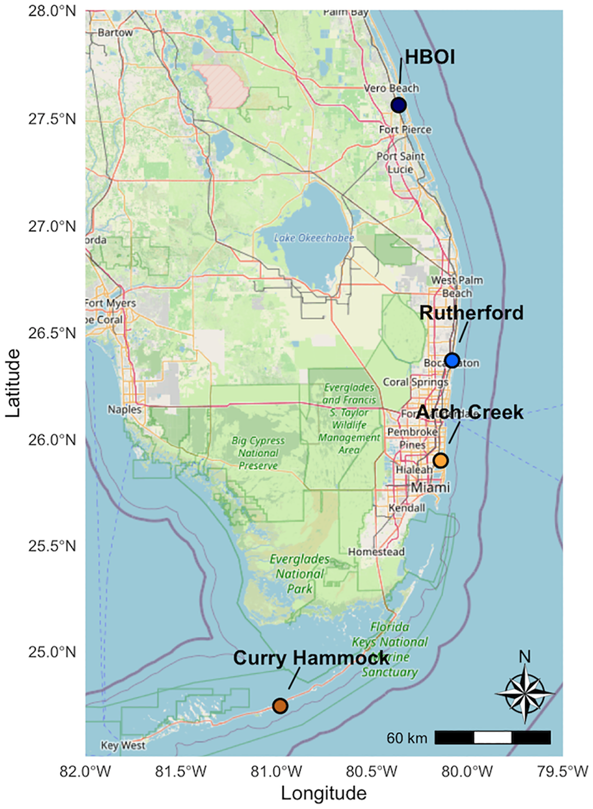
Geographical locations of the four experimental study sites located in Florida, USA: Curry Hammock (24.80°N, 80.70°W), Arch Creek (25.92°N, 80.19°W), Rutherford (27.27°N, 80.25°W), and Harbor Branch Oceanographic Institute (HBOI) (27.53°N, 80.34°W). Each site is depicted by a distinct color and labeled on an OpenStreetMap base layer, providing context for the study’s field locations.
At each site, five representative trees were selected. The trees were approximately 10–30 m apart, except in a few cases where structures interrupted a coastal stand. The tree characteristics measured were the trunk diameter at breast height of 1.3 m (referred to hereafter as DBH) and the prop root density in a 0.5-m × 0.5-m quadrat. Each of the five treatment types (the fixed factor) were randomly deployed at each block/tree (the random factor). The experiment utilized 10-cm2 polyvinyl chloride (PVC) panels acting as a control variable for the community development timescale, habitat area, surface type, and habitat type. There were five treatment types: open (to predators of all sizes), partial micro exclosure, partial macro exclosure, macro exclosure, and micro exclosure (Figure 2). Each treatment type was replicated five times. The panels were hung face down from the branches of the mangrove (R. mangle) trees at a height that allowed them to remain submerged throughout the majority of the tidal cycle. Predators potentially could reach these treatment panels via adjacent prop roots, but could not access the panels directly from the ground. Secondary foundation species naturally colonized the panels, and their presence was not controlled by manual removal or any other method. Positioning in reference to the current was not controlled for in the deployment of the panels. The predation exclosure treatments were randomly deployed within each block (tree), but care was taken to make sure that a deployment pattern was not repeated within a site.
Figure 2
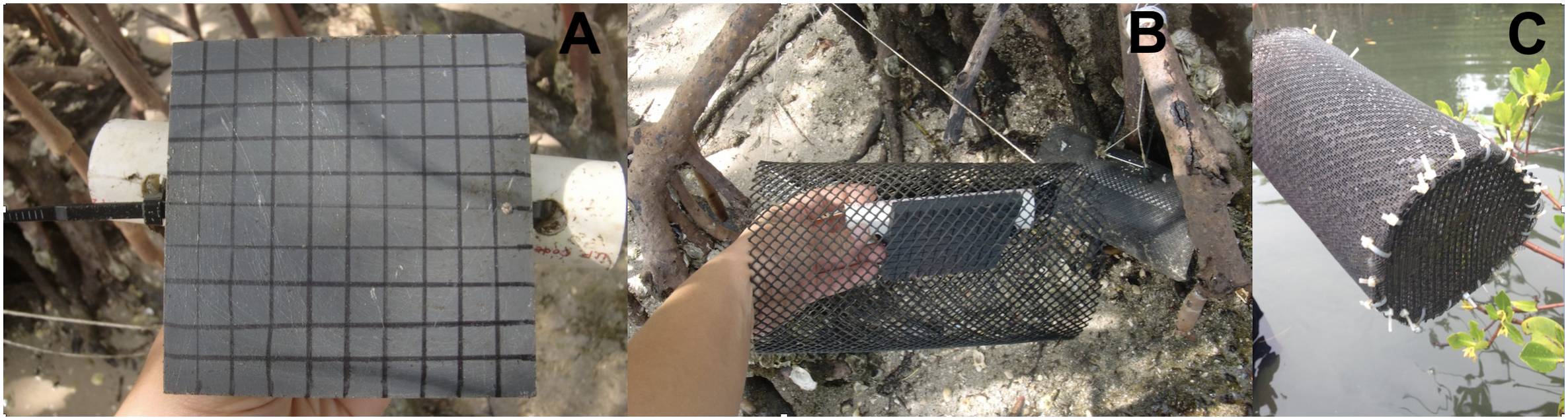
Colonization panel and experimental treatment types. This figure illustrates the different experimental treatment types used in the study, showcasing the 10-cm × 10-cm colonization panel common to all setups and the method of attachment. (A) Open treatment type: depicts the standard 10-cm × 10-cm colonization panel used in all the treatment types. A PVC piece zip-tied to the panel serves as the attachment point for rope connecting it to the experimental tree. This setup allows for access by all potential predators. (B) Partial macro treatment type: shows the 10-cm × 10-cm colonization panel enclosed within a cylindrical mesh exclosure. This exclosure is open at both ends, allowing for access by most predators, but perhaps excluding very large predators. (C) Micro exclosure treatment type: features the colonization panel inside the macro enclosure (as described below), which is further covered with a finer screen material. This design excludes both macrofauna and smaller microfauna predators, providing the highest level of exclusion. Note that the macro treatment type (not pictured) is identical to the partial macro enclosure, but has both ends closed off with the same mesh material, completely excluding macrofauna, but allowing access of micropredators. The partial micro treatment type (not pictured) is similar to the micro exclosure, but has both ends open, analogous to the partial macro design.
The predation exclosure treatment types used two mesh types (1 and 5 mm) in order to eliminate different predator guilds (Figure 2). The “macro” exclosure treatment was assembled from 5-mm plastic Vexar marine-grade mesh. This treatment type excluded large predators, but allowed micro-predators to enter. The “micro” exclosure treatment type was assembled by encasing the macro exclosure treatment type with a 1-mm fiberglass window screen. This treatment type should have eliminated or substantially reduced the micro-predators that were still able to access the panels in the macro exclosure treatment type. All treatment types were cleaned each time a site was visited in order to reduce fouling and to eliminate predators that may have gained access to the interior of the treatments during their larval stage. There were two partial treatment types: “partial macro” and “partial micro.” These treatment types consisted of a cylinder opened at each end, with the respective materials encircling the cylinder, but allowing the ends to remain open. The final treatment type, “open,” is a panel without any exclosure around it, therefore allowing all predators free access. The colonization panels (10–cm2, PVC) were deployed for each replicate of the treatment types. After 6 months, the panels were removed from the field sites and were examined using a dissecting microscope. The panels were assessed for species richness and percent cover. For species richness, all organisms were identified to the lowest possible taxonomic group. For percent cover, the Coral Point Count software was used to employ a stratified random 50-point count grid over the 10-cm2 PVC panels (Kohler and Gill, 2006).
At each tree, the water quality variables were documented using the YSI Professional Plus series. Water quality points were taken directly in front of each tree in a minimum water depth of 0.5 m. The following parameters were used in the models: turbidity, salinity, total dissolved solids, temperature, sigma S (density of the water), and dissolved oxygen. The YSI Professional Plus series provided several water quality variables, with a number of variables having multiple measurement units and/or co-varying strongly with each other. For instance, when this occurred, only one parameter was used for the analysis, e.g., for salinity, practical salinity unit (PSU), and specific gravity, only PSU was used.
Data analysis
The species richness, evenness (Pielou’s), biodiversity (Shannon–Wiener), and percent coverage for each panel were calculated from point counts at a range of scales and at each of the collection dates (fixed factor). A randomized complete block design with repeated measures was employed. The latitudinal gradient was separated into four zones, with one site (fixed factorial variable) per zone. Each of the five treatment types (fixed factor) were randomly deployed at each block/tree (random factor). The block/tree is the smallest sampling unit, comprising the replicates for the sites. A variable called “group“ was employed to analyze the effects of the predation exclosure treatment within each site. Group means were used for comparisons of the species richness, biodiversity, and percent coverage at each of the collection dates.
Prior to calculating community dissimilarities, the raw species abundance data, which included zero counts, were transformed to accommodate analytical methods that are sensitive to zero values and to prevent the loss of ecologically relevant samples. Specifically, a small constant, epsilon (ϵ), was added to every abundance value in the dataset. This transformation ensured that all values were positive, thus enabling the calculation of Bray–Curtis distance matrices, as well as the subsequent principal coordinates analysis (PCoA) and partial distance-based redundancy analysis (db-RDA). The inclusion of samples with zero counts is particularly critical in this predation experiment as zeroes are ecologically important, representing instances where a species was absent, potentially due to predation effects or environmental conditions. The chosen ϵ value was 0.0000001 and was selected to be small enough to minimally alter the relative differences between non-zero counts while preventing the exclusion of rows that would otherwise be lost if containing only zeroes. This approach allowed the retention of all samples, including those with zero counts, thereby preserving the ecological signal associated with species absences.
The effects of predation exclosure treatment, site, and the interaction between predation treatment and site were assessed using distance-based permutational multivariate analysis of variance (PERMANOVA). Analysis was based on the Bray–Curtis dissimilarities (Anderson, 2001a; Anderson, 2001b; Anderson et al., 2017) using species richness as the response variable. The model assessed with PERMANOVA consisted of three factors: site (fixed factor, with four levels), tree/block (random factor, with five levels nested within site), and treatment (fixed factor, with five levels, nested in tree/block) with 999 permutations. All tests were performed at a 5% level of significance. When significant differences were found (p < 0.05), a posteriori pairwise comparisons with 999 permutations among all levels of a fixed factor were also performed. PERMANOVA, similarly to ANOVA, detects differences in the mean value between treatment groups, and it tests that the distribution distance matrices of the groups are different. To assess the assumption of homogeneity of multivariate dispersions for PERMANOVA, PERMDISP (permutational multivariate analysis of dispersion) was performed using Bray–Curtis dissimilarities with 999 permutations.
Hierarchical clustering was used to look for patterns of relatedness of the groups (treatments nested within the sites). The Bray–Curtis dissimilarity index creates a matrix of percent difference dissimilarities between groups (Bray and Curtis, 1957). Bray–Curtis dissimilarity indices are used to quantify the differences between species populations between sites. Ward’s hierarchical clustering algorithm is a least-squares method. Minimum variance in clustering is achieved by the dissimilarities getting squared before cluster updating (Ward, 1963; Murtagh and Legendre, 2014).
To determine the most appropriate dissimilarity index to use for the PCoA and partial db-RDA (below), the rank index from the vegan package in R was used. This function calculated the rank correlation coefficients between various community dissimilarity indices and the environmental data used as a measure of gradient separation. The environmental data were scaled by dividing the centered value by the standard deviation. The Bray–Curtis dissimilarity distance matrices were consistently found to be the top metric distance for evaluation of the gradient separation. Due to the potential for negative eigenvalues when using non-Euclidean dissimilarities, a Lingoes correction was applied to the distance matrix.
Multivariate patterns were assessed using PCoA ordinations of the Bray–Curtis dissimilarities. PCoA uses orthogonal axes, for which importance is measured by eigenvalues to return points such that their distances are equivalent to their dissimilarities (Gower, 1966). Lingoes correction was used to ensure that the eigenvalues were not negative (Cailliez, 1983). A scree plot was completed for selection of the number of dimensions to include in the PCoA.
Constrained db-RDA was used to regress the effects of the environmental variables on the PCoA (Legendre and Anderson, 1999). In this analysis, the variables that explained most of the variation were determined via a stepwise permutation procedure (Legendre and Legendre, 2012). Using a Bray–Curtis distance-based matrix, partial db-RDA was performed using a forward model and a constrained global model. db-RDA is a constrained ordination that combines regression and PCoA. Partial db-RDA conditions the constrained ordination by one or more variables. For this research, group is the conditional variable, which is the predation treatment type within each site. The forward model was developed with an r2 significance cutoff of 0.05 using 999 permutations to produce the models. Significant predictor variables were included as biplots on the ordinations.
Forward modeling has been criticized as too liberal. To correct for this, the forward model can be compared against a constrained global model (Luo et al., 2006). For the constrained global model, variables are added with a limit such that the r2 is not higher than the adjusted r2 from the corresponding global model (Burnham and Anderson, 2002). The global model environmental variables were site characteristics, the human disturbance variables, tree characteristics, and the water quality variables. A global test, for the partial db-RDA, was performed on the dataset using the Lingoes-adjusted squared Bray–Curtis distance matrix that was created with the species data, the environmental data where the mean of the variables was divided by the standard deviation, and the conditional variable was the predation exclosure treatment type.
Both the db-RDA and partial db-RDA modeling methods were run with and without the secondary foundation species included in the environmental variables. The inclusion of secondary foundation species in the environmental variables allows for the secondary foundation species to be regressed against the PCoA results and for the shared biotic and abiotic factors on all species colonization to be described. Models and the significant values in each model were evaluated with an ANOVA using 1,000 permutations to assess the significance of the model and the model constraints (Legendre et al., 2011). Partial db-RDA allows for one variable to be the condition on which the db-RDA is run. The conditional variable used was the treatment variable, i.e., the predation exclosure treatment type. Consequently, the effects of the variable can be separately measured in the analysis.
In addition, pairwise Spearman’s rank correlations were run to estimate the strength of the relationship between each foundation species for each treatment type at each site. Spearman’s rank correlation is a multidimensional statistical technique that can be used to assess the relationship between descriptors, providing the strength and the direction of the relationship. The significance was set to 0.05. All statistical analyses and data visualization were completed using base R (v. 4.1.1) and the following packages: vegan (v. 2.6-4), BiodiversityR (v. 2.17-2), tidyverse (v. 2.0.0), sf (v. 1.0-21), ggspatial (v. 1.1.9), rstatix (v. 0.7.2), and ggrepel (v. 0.9.6) (Kindt and Coe, 2005; Oksanen et al., 2025; Wickham et al., 2019; Dunnington, 2023; Pebesma, 2023; R Core Team, 2025).
Results
Initial deployments of the treatments at each site were completed in June 2015. Throughout the field experiment, a total of 62 species were recorded. From south to north, 17 species were observed at Curry Hammock, 37 at Arch Creek, 42 at Rutherford, and 27 at HBOI. In the southern half of the experimental zone, sponge and ascidian species were more prevalent, regardless of treatment type. Tropical species such as the sponge (Dysidea etheria) and several Botrylloides ascidian species were absent at the northernmost site, while temperate species such as the eastern oyster (Crassostrea virginica) were not found at the southernmost site.
Species richness was assessed during the three sampling periods. The first data collection point (approximately 1 month after deployment) identified 33 species. The subsequent data collection, which was restricted to Rutherford and HBOI, yielded 30 species. The last data collection point (November and December) recorded the highest species richness, with 51 species. The total species richness over the length of the entire experiment was further examined by treatment within each site (Table 1). At all sites, an increase in species richness was observed over the course of the study: Curry Hammock, from 3 to 17; Arch Creek, from 25 to 32; James Rutherford, from 14 to 30; and HBOI, from 9 to 17. The total species richness at the end of the study was further examined by treatment within each site (Table 2).
Table 1
| Site | Predation exclosure treatment | ||||
|---|---|---|---|---|---|
| Open | Partial macro | Partial micro | Macro | Micro | |
| Curry Hammock | 8 | 10 | 9 | 11 | 7 |
| Arch Creek | 24 | 29 | 27 | 16 | 22 |
| Rutherford | 22 | 19 | 27 | 20 | 20 |
| HBOI | 12 | 11 | 10 | 17 | 18 |
Total species richness at each site over the length of the whole experiment by predation exclosure treatment type.
Sites are listed south to north (top to bottom).
HBOI, Harbor Branch Oceanographic Institute.
Table 2
| Site | Predation exclosure treatment | ||||
|---|---|---|---|---|---|
| Open | Partial macro | Partial micro | Macro | Micro | |
| Curry Hammock | 7 | 10 | 9 | 10 | 7 |
| Arch Creek | 21 | 25 | 22 | 16 | 19 |
| Rutherford | 15 | 15 | 16 | 17 | 10 |
| HBOI | 6 | 6 | 5 | 7 | 13 |
Total species richness at each site at the end of the experiment by predation exclosure treatment type.
Sites are listed south to north (top to bottom).
HBOI, Harbor Branch Oceanographic Institute.
Predation produced opposite effects at either end of the extremes of the latitudinal gradient: increasing species richness (Figure 3) in the north and less clearly reducing species richness in the south. Species richness was initially highest in Arch Creek, the transition zone, and remained the highest over the course of the study. Interestingly, at this site, initially, the exclosures that prevented access of at least some predators had the highest species richness; however, by the end of the study, they had the lowest species richness at the site. The southernmost site, Curry Hammock, had the lowest initial species richness and a weak current flow at the site, as it was situated snugly between two keys, Long Point Key and Little Crawl Key, likely contributing to the results more than any experimental factor.
Figure 3
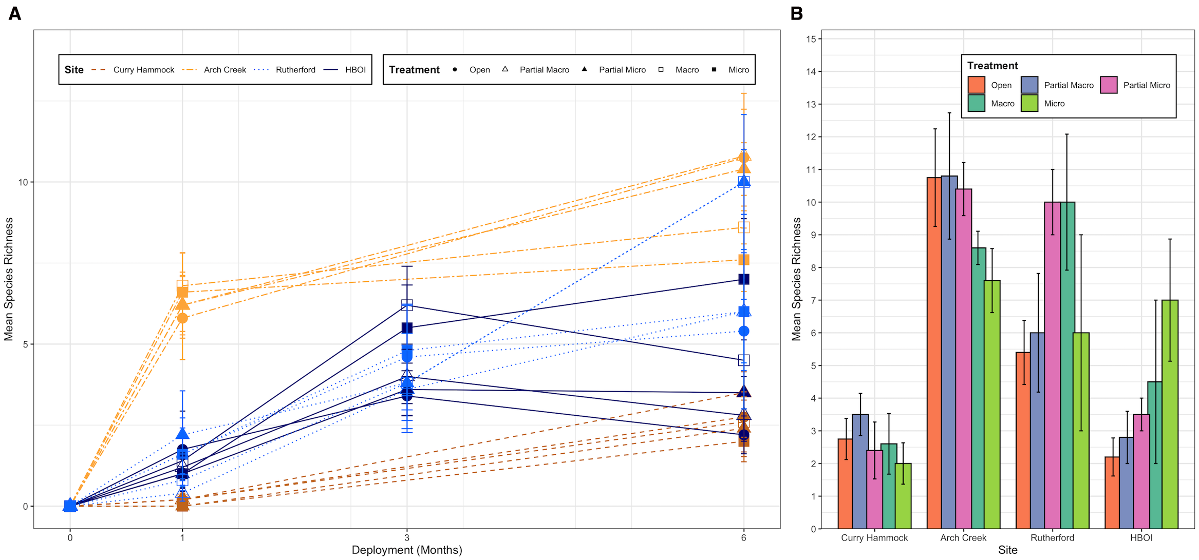
Mean species richness at each site by predation exclosure treatment type. (A) Mean species richness over the deployment (6 months) by site and treatment. Line represents the change in the mean species richness across deployment (months 0, 1, 3, and 6). Each line corresponds to a unique combination of site (distinguished by color and line type) and treatment (distinguished by point shape). Data points show the mean species richness for each site–treatment–deployment combination. Error bars indicate the standard error of the mean (SE). (B) Bar chart illustrating the mean species richness observed at the sites under different treatment conditions at the end of the study (6 months). Error bars represent the SE of the mean species richness for each site and treatment combination. Site shown going south to north: Curry Hammock, Arch Creek, Rutherford, and Harbor Branch Oceanographic Institute (HBOI).
Community diversity was also measured using Shannon–Wiener. A comparison of the treatment types over the latitudinal gradient found that the open treatment type had lower diversity values in the northern half of the study when compared with its protected treatment exclosure counter type, while in the south, the predation did not have as clear of an affect. In the northern half of the study, certain soft-bodied species were not observed, unless they were in macro- and/or micro-predation exclosures (Figure 4). The Shannon–Wiener for the initial data collection visit across all sites was 2.69; for the second data collection (which did not include two sites, Curry Hammock and Arch Creek), it was 2.199. The biodiversity for the end of the experiment across all sites had a Shannon–Weiner measure of 2.402: 2.244 for Curry Hammock, 2.716 for Arch Creek, 2.171 for Rutherford, and 0.900 for HBOI. The Shannon–Weiner at the end of the study was further parceled out by treatment within each site (Figure 4). Overall, Arch Creek had the highest diversity, and abundance was more evenly distributed (Pielou’s evenness: Curry Hammock, 0.544; Arch Creek, 0.658; Rutherford, 0.526; HBOI, 0.218). On the other hand, HBOI had one or a few dominant species. However, the HBOI micro exclosure treatment type broke with the trend and had an appreciably higher species evenness (open = 0.064, partial macro = 0.132, partial micro = 0.189, macro = 0.163, and micro = 0.446). Measures of pairwise dissimilarity can have limited usefulness when the local species richness is very low in comparison to the regional species richness.
Figure 4
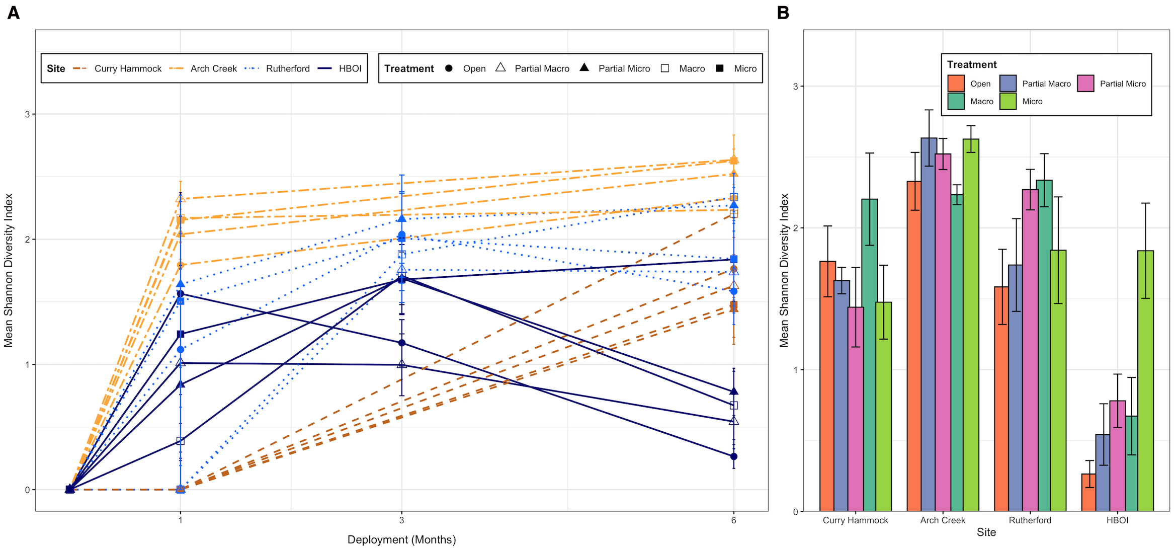
Mean Shannon–Weiner value at each site by predation exclosure treatment type. (A) Shannon diversity index over deployment by site and treatment. Lines represent the mean Shannon diversity index observed across deployment (months 0, 1, 3, and 6). Each unique combination of site (distinguished by color and line type) and treatment (distinguished by point shape) is shown. Error bars indicate the standard error of the mean (SE). (B) Bar chart illustrating the mean Shannon diversity index observed at the sites under different treatment conditions at the end of the study (6 months). Error bars represent the SE of the mean Shannon diversity index for each site and treatment combination. Site shown going south to north: Curry Hammock, Arch Creek, Rutherford, and Harbor Branch Oceanographic Institute (HBOI).
Arch Creek had one treatment type, i.e., macro exclosure, which did not see a change in its mean Shannon–Weiner value. This appears to have been in relation to the species abundance/percent cover as the species richness for the macro exclosure treatment increased over the same time span. Over the course of the study, HBOI, not including the micro exclosure treatment type, had a decrease in its Shannon–Weiner value. The final HBOI micro exclosure treatment had values that were within the range of the next site to the south, Rutherford, demonstrating the important impact of micro-predation at HBOI.
The initial colonization, from deployment to 1 month later, at Curry Hammock was extremely low. Arch Creek had the highest initial overall biodiversity, with all the treatment types exhibiting high values. At James Rutherford Park, things were a little more difficult to interpret, with three of the treatment types having high initial biodiversity and two having some of the lowest. The three treatment types—open, partial micro, and micro exclosures—had high biodiversity indices and saw a moderate reduction in biodiversity in the next collection date. Conversely, the James Rutherford macro exclosure and partial macro treatment types saw an increase in biodiversity over the course of the field experiment, with the macro exclosure treatment ending up having the highest diversity for the site. The initial diversity in colonization for the treatments at HBOI was similar for all treatment types, except for the macro exclosure treatment (Figure 4A). At the end of the study, the HBOI site saw a further decrease in biodiversity for all treatment types, except for the micro exclosure treatment, which mimicked the species richness’ increasing slope, likely due to an increase in the number of species present. The combined pressure of macro- and micro-predation in the temperate zone had significantly decreased species richness (Figure 3).
At the conclusion of the experiment, the Shannon–Weiner values were largest for Arch Creek, the transition zone (Figure 4B). There was a decrease in biodiversity heading north to Rutherford, although there was a substantial overlap in biodiversity between the two sites. At Rutherford, the macro-predation exclosure treatment was the treatment with the highest biodiversity. The last site along the latitudinal gradient had the lowest biodiversity, with four of the treatments showing a drastic drop in diversity (Figure 4). At HBOI, the micro exclosure treatment was the only treatment that did not follow the trend, instead retaining a biodiversity that was extremely close to the Rutherford micro exclosure biodiversity and higher than the Rutherford open biodiversity. When HBOI was released from both micro- and macro-predation, the Shannon–Wiener value was within the values found for the next site to the south. Again, micro-predation appears to be a factor limiting biodiversity in the temperate zone of the experiment. The biodiversity at Curry Hammock is largely an artifact of the weak water flow at the site.
PERMANOVA was conducted using Bray–Curtis dissimilarities to examine the effects of site and predation exclosure treatment on the community composition, with 999 permutations (Table 3). Before interpreting the PERMANOVA results, a test for homogeneity of multivariate dispersions (PERMDISP) was performed using the same Bray–Curtis dissimilarity matrix to ensure that the differences in the location of the group centroids were not confounded by the differences in group variability. PERMDISP revealed a significant difference in the multivariate dispersion among the four sites (Pseudo-F = 19.499, df = 3, 78, p = 0.001). Pairwise PERMDISP tests indicated that all site comparisons were statistically significant (p ≤ 0.004), except for the comparison between Arch Creek and Rutherford (p = 0.251). These significant dispersion differences among sites suggest that the interpretation of the site effects from the PERMANOVA should be made with caution, as differences in the community composition between sites could be influenced by varying levels of within-group heterogeneity. PERMDISP was conducted for the treatment factor using the same Bray–Curtis dissimilarity matrix. The results of this test revealed no significant differences in the multivariate dispersion among the five treatment groups (Pseudo-F = 0.402, df = 4, 77, p = 0.8), suggesting that the variability within the treatment groups is similar. This finding increases confidence in the observed significant effect of treatment found in the PERMANOVA. The PERMDISP for the treatment within each site revealed a significant difference in the multivariate dispersion among the four sites (Pseudo-F = 3.825, df = 19, 62, p = 0.001).
Table 3
| Treatment comparison | All sites | Curry Hammock | Arch Creek | Rutherford | HBOI |
|---|---|---|---|---|---|
| Open vs. partial macro |
F = 4.69 R2 = 0.53 p = 0.503 |
F = 1.28 R2 = 0.18 p = 0.394 |
F = 0.55 R2 = 0.07 p = 0.779 |
F = 0.74 R2 = 0.08 p = 0.640 |
F = 1.48 R2 = 0.16 p = 0.307 |
| Open vs. partial micro |
F = 4.05 R2 = 0.54 p = 0.214 |
F = 1.68 R2 = 0.19 p = 0.079 |
F = 1.31 R2 = 0.16 p = 0.201 |
F = 0.54 R2 = 0.10 p = 0.513 |
F = 3.27 R2 = 0.40 p = 0.144 |
| Open vs. macro |
F = 4.73 R2 = 0.57 p = 0.016* |
F = 0.62 R2 = 0.08 p = 0.730 |
F = 5.31 R2 = 0.43 p = 0.010** |
F = 3.06 R2 = 0.34 p = 0.054* |
F = 2.69 R2 = 0.35 p = 0.095 |
| Open vs. micro |
F = 3.36 R2 = 0.48 p = 0.038* |
F = 0.68 R2 = 0.09 p = 0.703 |
F = 2.17 R2 = 0.24 p = 0.030* |
F = 0.91 R2 = 0.15 p = 0.414 |
F = 5.89 R2 = 0.46 p = 0.019* |
| Partial macro vs. partial micro |
F = 3.06 R2 = 0.46 p = 0.996 |
F = 0.40 R2 = 0.05 p = 1.000 |
F = 0.75 R2 = 0.09 p = 0.752 |
F = 0.29 R2 = 0.05 p = 0.915 |
F = 0.34 R2 = 0.06 p = 0.598 |
| Partial macro vs. macro |
F = 3.64 R2 = 0.50 p = 0.051 |
F = 0.81 R2 = 0.10 p = 0.659 |
F = 3.33 R2 = 0.29 p = 0.008** |
F = 1.82 R2 = 0.23 p = 0.174 |
F = 0.53 R2 = 0.10 p = 0.640 |
| Partial macro vs. micro |
F = 2.65 R2 = 0.41 p = 0.186 |
F = 1.13 R2 = 0.14 p = 0.321 |
F = 1.26 R2 = 0.14 p = 0.233 |
F = 0.39 R2 = 0.07 p = 0.724 |
F = 3.58 R2 = 0.34 p = 0.026* |
| Partial micro vs. macro |
F = 2.78 R2 = 0.48 p = 0.017* |
F = 1.14 R2 = 0.12 p = 0.248 |
F = 4.32 R2 = 0.35 p = 0.008** |
F = 1.16 R2 = 0.28 p = 0.400 |
F = 0.40 R2 = 0.17 p = 1.000 |
| Partial micro vs. micro |
F = 1.96 R2 = 0.38 p = 0.337 |
F = 1.49 R2 = 0.16 p = 0.176 |
F = 1.53 R2 = 0.16 p = 0.205 |
F = 0.24 R2 = 0.11 p = 1.000 |
F = 1.20 R2 = 0.23 p = 0.267 |
| Macro vs. micro |
F = 2.10 R2 = 0.39 p = 0.539 |
F = 0.56 R2 = 0.07 p = 0.860 |
F = 1.51 R2 = 0.16 p = 0.185 |
F = 0.62 R2 = 0.17 p = 0.900 |
F = 1.52 R2 = 0.27 p = 0.267 |
Results of the pairwise permutational multivariate analysis of variance (PERMANOVA) comparisons, using Bray–Curtis dissimilarity, between the different predation exclosure treatments (open, partial cage, partial screen, cage, and screen) within each specified site and across all sites combined.
The between-site comparison was run with the treatments nested within their respective sites. Each cell reports the pseudo-F statistic (F), the R2 value, and the p-value for the respective comparison. Statistical significance is indicated by asterisks attached to the p-value.
*p ≤ 0.05; **p ≤ 0.01.
PERMANOVA revealed that both site and predation exclosure treatment significantly influenced the community composition. The effect of the sites was stronger (Pseudo-F = 12.347, df = 3, 78, R2 = 0.322, p = 0.001) than that of the predation exclosure treatment (Pseudo-F = 1.569, df = 4, R2 = 0.0754, p = 0.001). Pairwise comparisons among the four sites were then performed to identify specific differences. All pairwise comparisons were statistically significant at p ≤ 0.002. Site explained approximately 32.2% of the total variation in community composition. However, even accounting for the site-specific differences, treatment still had a statistically significant influence on the community structure. Further pairwise tests for the nested effect of treatment within each site were completed. The comparison of open vs. macro (Pseudo-F = 4.734, df = 7, 78, R2 = 0.570, p = 0.021) and open vs. micro (Pseudo-F = 3.361, df = 7, 78, R2 = 0.475, p = 0.039) were significant across all sites. Macro was also nearly significantly different from partial macro (Pseudo-F = 3.644, df = 7, 78, R2 = 0.495, p = 0.061) and was significantly different from partial micro (pseudo-F = 2.78, df = 7, 78, R2 = 0.481, p = 0.016). Micro was not significantly different from either partial exclosure.
The variability in the F and R2 values across sites for the same treatment comparison suggests that the impact of predation exclosure treatments is not uniform across all locations. Local environmental conditions and/or other site-specific factors likely modify how treatments affect the community. A larger F-value suggests a greater difference between groups. For example, the open vs. cage comparison is strongest in Arch Creek (F = 1.66), followed by Rutherford (F = 1.42) and HBOI (F = 1.26), and was weakest (and not significant) in Curry Hammock (F = 0.75) at the end of the study. The comparison between open, macro, and micro were frequently significant in Arch Creek, Rutherford, and HBOI. Arch Creek also had the most significant treatment differences, suggesting that its communities might be more sensitive to the predation exclosure treatments compared with the other sites (Table 3).
In general, there was a trend of increasing percent coverage toward the north. Coverage started low and remained lowest at Curry Hammock, the southernmost site. Arch Creek had the highest initial colonization. The two northernmost sites, Rutherford and HBOI, both had a relatively low initial colonization and a high final percent coverage (Figure 5). The percent cover was low where the species richness was low and was high where the species richness was high, except at HBOI, which had the highest percent coverage by predation exclosure treatment type. This deviation is likely due to shelled specimens leaving behind hard structures upon death and the percent coverage data unable to separate live versus dead specimens.
Figure 5
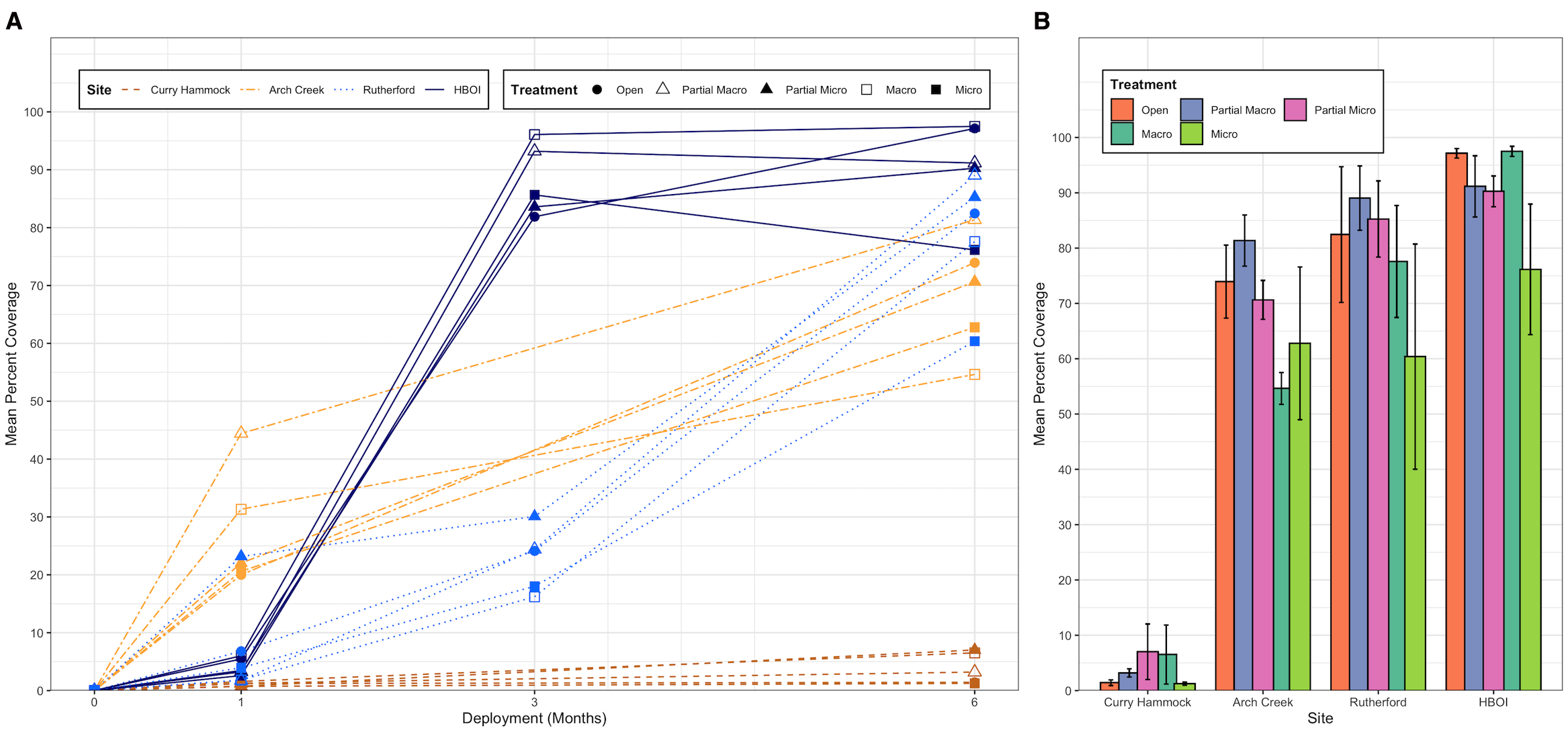
Mean percent coverage at each site by predation exclosure treatment type. (A) Mean percentage coverage by site and treatment over the deployment of the colonization panels. Lines depict the change in the mean percentage coverage across the different deployment times (months 0, 1, 3, and 6). Each line represents a unique combination of site (identified by color and line type) and treatment (identified by point shape). Data points show the mean percentage coverage for each site–treatment–deployment combination. Error bars representing the standard error (SE) were omitted for clarity due to the high density of the lines. (B) Mean percentage coverage by site and treatment type at the end of the study (6 months). Bar heights represent the mean percentage coverage observed for each treatment type within the four different sites [going south to north: Curry Hammock, Arch Creek, Rutherford, and Harbor Branch Oceanographic Institute (HBOI)]. Each site is shown on the x-axis, with bars grouped by treatment (open, partial macro, partial micro, macro, and micro), distinguished by fill color as indicated in the legend. Error bars represent the SE of the mean.
Hierarchical clustering was used to assess differences in the community assemblages between the groups, treatments nested within the sites. Overall, the sites clustered along the latitudinal gradient (Figure 6). Clusters were based on the relatedness of the species composition of the treatments within the sites. The open treatment type, which allowed for full predator access, followed the expected latitudinal gradient. Overall, the predation exclosure treatment types clustered within the specific site. Only one treatment did not cluster with the other treatments within its site. Removal of all predation at HBOI, the northernmost site, resulted in an epifaunal community that was more similar to that in the site to the south than to that in treatments within the site.
Figure 6
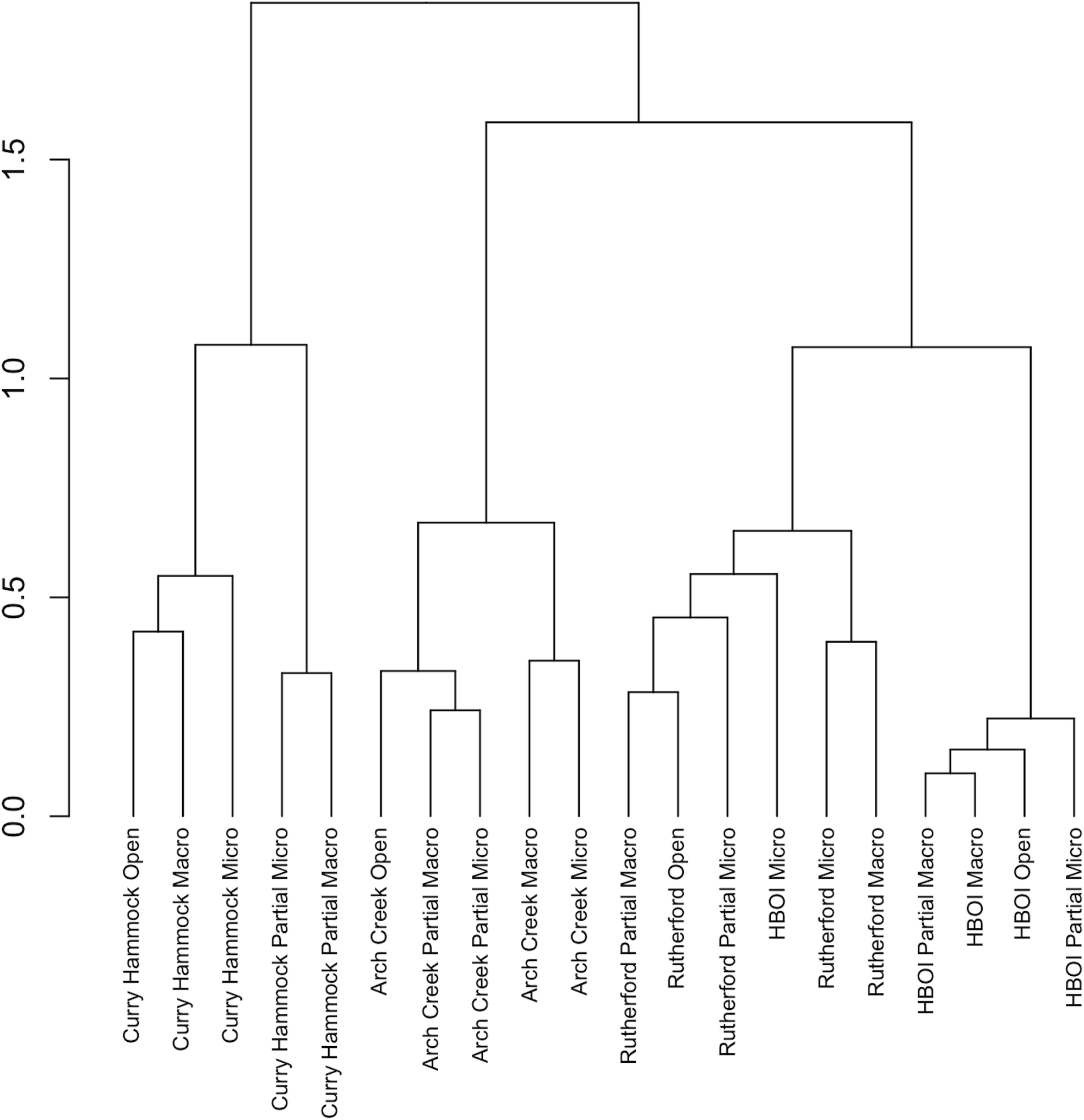
Hierarchical clustering dendrogram of site and treatment combinations based on the Bray–Curtis dissimilarity. Ward’s hierarchical clustering algorithm was used to produce a hierarchical dendrogram for the sites and treatment exclosure type combinations based on species presence. The vertical axis represents the Bray–Curtis dissimilarity at which the site treatment combination merged. The horizontal axis represents the individual site treatment combinations grouped according to their compositional similarities.
The PCoA confirmed the hierarchical clustering of the treatments within the sites, with site remaining as the primary clustering criterion. The first two dimensions of the PCoA accounted for 28.5 of the goodness of fit, the amount of variation captured. PCoA, which included secondary foundation species in the analysis with the epifaunal community, revealed that Curry Hammock did not have any overlap with the other sites (Figure 7). Points closer together on the plot are more similar in community composition according to the Bray–Curtis dissimilarity matrix used. Rutherford’s ellipse overlapped with both HBOI, the site to the north, and Arch Creek, the site to the south. The standard deviation ellipse for HBOI was entirely nested within the ellipse for Rutherford and did not overlap with the ellipse from Arch Creek. This indicates that while Rutherford exhibited a broader range of community compositions, the entire observed variation of the HBOI communities was contained within that larger range. This included the screen treatment type for HBOI that fell outside its standard deviation ellipse, but still within the Rutherford ellipse. For the site to the south, Arch Creek, Rutherford’s macro exclosure clustered closely due to more shared species. The standard deviation ellipse for Rutherford was positioned such that it largely encompassed or significantly overlapped with the ellipse for Arch Creek, suggesting a high degree of similarity in the community composition between these two groups, despite their different geographical locations.
Figure 7
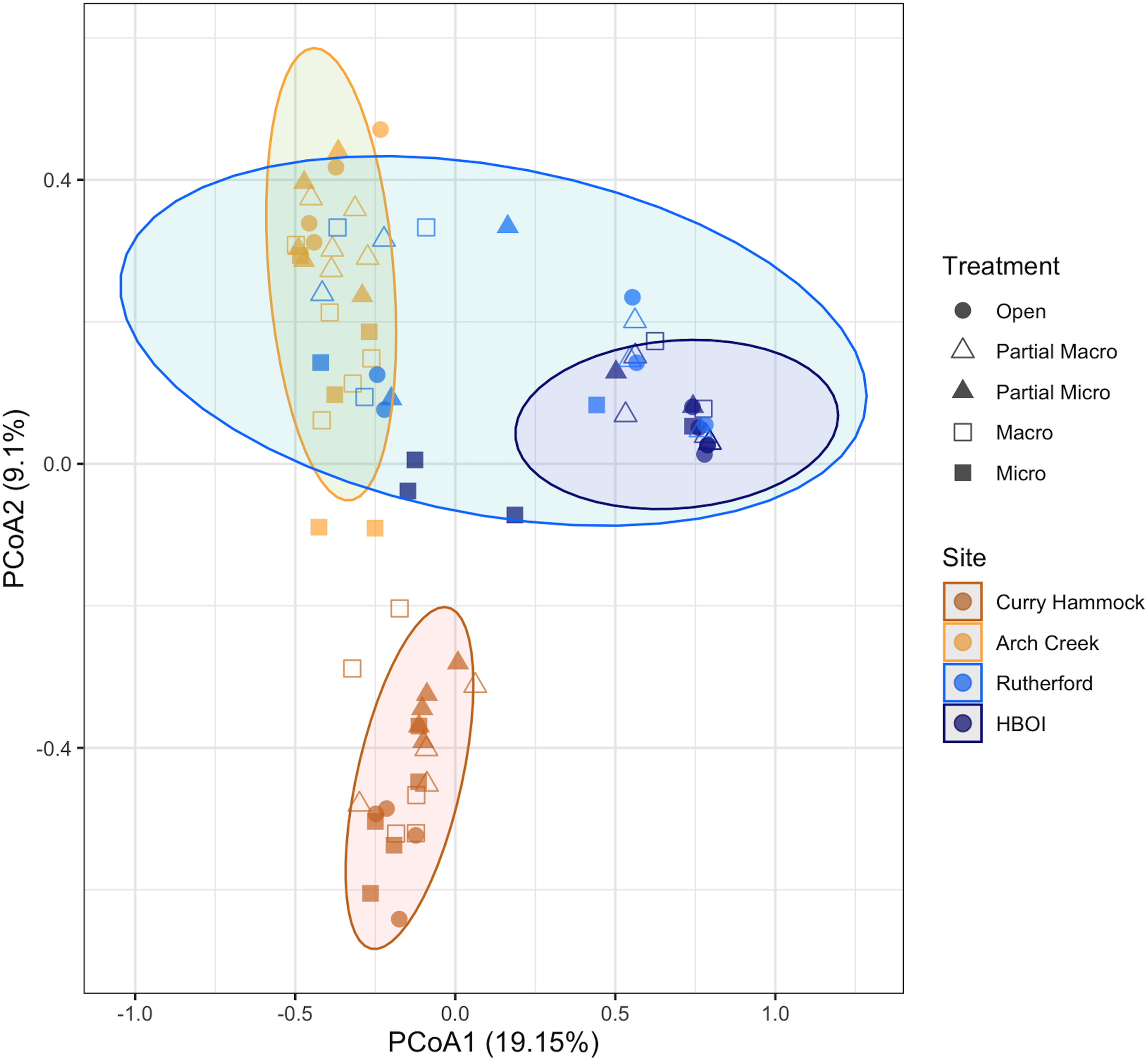
Ordination of the principal coordinates analysis (PCoA) of the benthic community composition (including secondary foundation species) based on the Bray–Curtis distance matrix. Bray–Curtis dissimilarity, a measure of beta diversity, quantifies the difference in species composition between samples based on the relative abundance. Data represent the summed species counts for the last data collection aggregated by site, treatment, and group. Ovals represent the standard deviation for each site. Colors coincide with sites and shapes with the treatment type. The first axis (PCo1) explained 19.15% of the total variation, while the second axis (PCo2) explained 9.1%.
Within the Arch Creek site, distinct patterns of community dispersion were observed across treatment types (Figure 7). Samples from the open treatment type clustered relatively closely together, indicating a higher degree of similarity in their community composition. In contrast, samples from the macro treatment type showed a greater spread, suggesting increased variability among these samples. This pattern of increasing dispersion continued with the micro treatment type, which exhibited the largest spread of points, reflecting the highest level of heterogeneity in community composition within that predation exclosure treatment at Arch Creek. These differences in the within-group variability were visually supported by the sizes of the corresponding standard deviation ellipses, which expanded progressively from open to macro to micro treatments at this site (Supplementary Figure S1).
A global test for the partial db-RDA was performed with predation exclosure type as the conditional variable. The model score was significant (F = 1.93, df = 18, 59, p < 0.001), indicating that the constrained model significantly explains the variation in species composition. This species composition did not include the secondary foundation species in the model. The analysis revealed a total inertia of 59.13, with 5.03% (2.97) explained by the conditional term (predation exclosure type) and 35.19% (20.81) explained by the environmental constraints. The remaining 59.78% (35.35) represented unconstrained inertia. The eigenvalues for the constrained axes ranged from 6.16 (CAP1) down to 0.35 (CAP18), while the unconstrained axes showed eigenvalues ranging from 4.41 (MDS1) to 0.66 (MDS8). The model’s explanatory power, as indicated by the adjusted R2, was 0.178, meaning that approximately 17.8% of the variation in species composition can be explained by the constrained environmental variables after accounting for the number of predictors in the model. This value suggests that the included environmental factors explain a moderate portion of the variability observed in the species data.
The constrained global model (adjusted R2 model), using the Bray–Curtis matrix, had the constrained inertia decrease to 19.34% (11.43), and the unconstrained inertia in turn increased to 75.63 (44.72), which included three environmental variables (Figure 8). When added to the model, salinity explained 8.65% of the adjusted variation (adjusted R2 = 0.0865). This addition was statistically significant (F = 8.29934, p < 0.001). Latitude further improved the model fit, increasing the adjusted R2 to 0.1654. Its contribution was also statistically significant (F = 8.18772, p < 0.001). The final variable added, Disturbance.Docks, increased the adjusted R2 to 0.1712, with a statistically significant contribution (F = 1.52661, p = 0.044). Ultimately, the model including salinity, latitude, and Disturbance.Docks explained an adjusted 17.83% of the variation in species composition (adjusted R2 = 0.1783). The eigenvalues for the constrained axes were 5.86 (CAP1), 4.93 (CAP2), and 0.65 (CAP3), representing the amount of variance explained by each axis. The eigenvalues for the unconstrained axes, which represent the remaining unexplained variation, ranged from 5.60 (MDS1) to 0.72 (MDS8). Further permutation tests were conducted to evaluate the significance of each canonical axis individually, holding all previous axes as conditions. The first constrained axis (salinity) was statistically significant (F = 9.69, df = 1, 74, p < 0.001), as was the second constrained axis (latitude; F = 8.15, df = 1, 74, p < 0.001). However, the third constrained axis (Disturbance.Docks) was not found to be statistically significant (F = 1.07, df = 1, 74, p = 0.299). These results suggest that the primary gradients of the environmental variation influencing species composition are captured by the first two CAP axes.
Figure 8
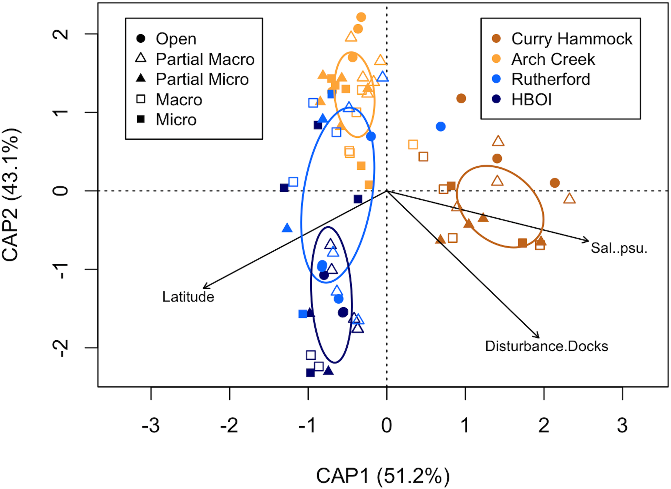
Partial distance-based redundancy analysis (db-RDA) based on species composition at the end of the study (not including secondary foundation species) using the Bray–Curtis distance matrix with Lingoes adjustment. The plot illustrates the relationship between sites (points), the conditional effect of treatment (accounted for first), and the environmental variables identified through forward selection. Environmental data had the mean of the variables divided by their standard deviation. The ellipses represent one standard deviation around the centroid for each site. Colors coincide with sites and shapes with the treatment type. The modeled environmental variables are shown as black biplots, which are drawn in reference to their association with the sites. The model explained an adjusted 17.83% of the variation in species composition. CAP1 and CAP2 represent the first two constrained axes and their proportions.
The inclusion of secondary foundation species in the environmental matrix for the partial db-RDA was revealed to be a significant model after a permutation test for the significance of the overall constrained model was performed using 999 permutations (F = 1.93, df = 18, 59, p < 0.001), with a total inertia of 59.13 and an adjusted R2 of 0286. The conditional term, treatment (predation exclosure type), accounted for 5.03% (2.97) of the total variation. The constrained environmental variables explained a substantial portion of the variation, accounting for 45.65% (26.99) of the total inertia. The eigenvalues for the 21 constrained axes ranged from 8.05 (CAP1) down to 0.33 (CAP21). The unconstrained axes showed eigenvalues ranging from 4.03 (MDS1) to 0.54 (MDS8).
The constrained global model with secondary foundation species in the environmental variables, using the Bray–Curtis matrix, included four variables in the model, each of which improved the model’s explanatory power. Addition of the secondary foundation species barnacle resulted in an adjusted R2 of 0.119 (F = 11.40, p < 0.001), salinity increased the adjusted R2 to 0.213 (F = 10.15, p < 0.001), the secondary foundation species sponge resulted in an adjusted R2 of 0.252 (F = 4.86, p < 0.001), and the secondary foundation species oyster brought the adjusted R2 to 0.279 (F = 3.80, p < 0.001) (Figure 9). This model explained 30.09% (17.79) of the total inertia (59.13). The conditional term accounted for 5.03% (2.97) of the total inertia. The remaining 64.88% (38.37) represented unconstrained inertia. The four variables, along with the conditional treatment term (predation exclosure), collectively explained an adjusted R2 of 0.286, suggesting that these variables are particularly important in structuring the community patterns. The eigenvalues for the four constrained axes were 7.97 (CAP1), 6.03 (CAP2), 2.67 (CAP3), and 1.12 (CAP4). The unconstrained axes showed eigenvalues ranging from 5.45 (MDS1) to 0.60 (MDS8). Further permutation tests were conducted to evaluate the significance of each canonical axis individually, holding all previous axes as conditions. All four constrained axes were found to be statistically significant. The first constrained axis (barnacle) was highly significant (F = 15.17, df = 1, 73, p < 0.001). The second (salinity; F = 11.47, df = 1, 73, p < 0.001), the third (sponge; F = 5.08, df = 1, 73, p < 0.001), and the fourth constrained axis (oyster) also showed a significant contribution (F = 2.14, df = 1, 73, p = 0.003). These results indicate that each of the four identified environmental gradients captured distinct and significant patterns in species composition. Moreover, the addition of secondary foundation species to the environmental variables increased the ability to model the system.
Figure 9
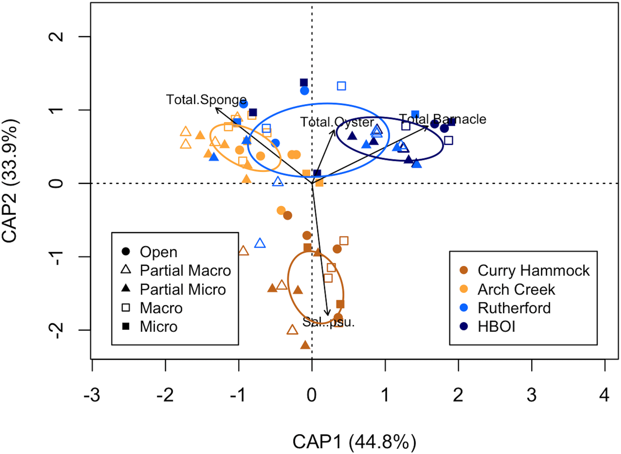
Partial distance-based redundancy analysis (db-RDA) based on species composition at the end of the study, with secondary foundation species in the environmental matrix, using the Bray–Curtis distance matrix with Lingoes adjustment. Environmental data had the mean of the variables divided by their standard deviation. The ellipses represent one standard deviation around the centroid for each site. Colors coincide with sites and shapes with the treatment type. The modeled environmental variables are shown as black biplots, which are drawn in reference to their association with the sites. The model explained an adjusted 28.56% of the variation in species composition. CAP1 and CAP2 represent the first two constrained axes and their proportions.
The association between secondary foundation species and predation changed along the latitudinal gradient. The relationship between secondary foundation species and associated species was not uniform across latitudes, suggesting context-dependent ecological dynamics. To investigate the relationship between species richness and the abundance of secondary foundation species, Spearman’s rank correlation was run for each treatment type. Overall, the strength and direction of the relationship between species richness and secondary foundation species varied a considerable amount based on the different predation exclosure treatment types (Figure 10). A few of the pairwise comparisons were significant, which is likely a result of the low power that occurred due to replicates, specifically at Rutherford and HBOI, being lost by the final visit of the experiment. Regardless, the site-specific relationship strength and patterns between the secondary foundation species and the associated species can be observed. At the southernmost site, Curry Hammock, the two secondary foundation species present—sponge and barnacles—although not significant, almost exclusively had positive relationships with species richness. At the next site to the north, Arch Creek, the patterns regarding the relationship between secondary foundation species and species richness were more varied. Sponges appeared to have a negative relationship with species richness in the fully enclosed predation exclosure treatment type, while the treatments with reduced predation had a positive relationship between species richness and sponge cover. This pattern, for the most part, was reversed when oysters were the secondary foundation species. There did not appear to be any discernible pattern between richness and barnacle cover.
Figure 10
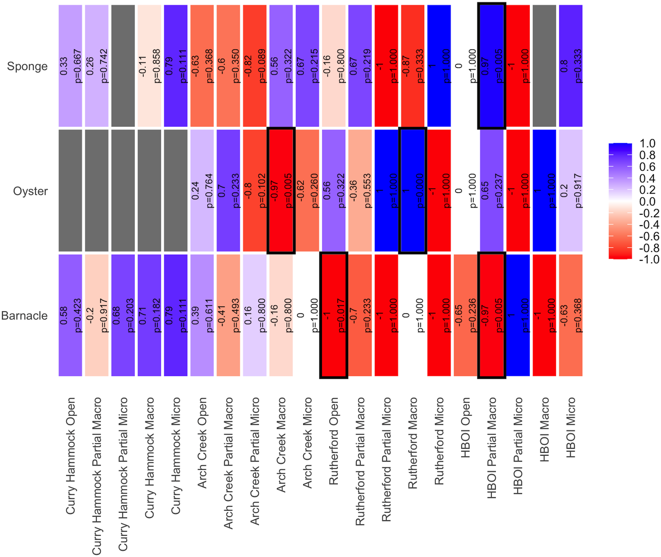
Heat map of the estimated correlation between each foundation species and the species richness for each treatment netted in each site. Sites are listed south to north. The pairwise Spearman’s rank correlation results for each correlation are shown in their respective boxes. Correlations with a significant p-value of <0.05 are highlighted with a black box around them. Cell colors represent the strength and direction of the correlation (blue = positive, red = negative). Empty cells indicate insufficient data for correlation calculation.
In the northern half of the experiment, the association with secondary foundation species became more varied and species-dependent. At Rutherford, sponges had a very strong positive relationship with species richness for the micro exclosure treatment type. Oysters, on the other hand, appeared to have the opposite correlation, reducing the species richness when all predators were excluded and increasing the species richness in the open and macro exclosure treatment types. Here, barnacles either had no correlation or had a negative correlation with species richness. At the northernmost site, HBOI, there was no effect of sponges or oysters on the species richness when all predators were permitted (open treatment), but a positive relationship when small and large predators (micro exclosure) were excluded. Oysters also had a positive relationship when only larger predators (macro exclosure) were excluded. Barnacles at the HBOI site typically had a negative relationship across the majority of the treatment types. The barnacle percent coverage was very high at the HBOI site; thus, colonization by other benthic species would be limited. Moreover, overall, barnacles exhibited a trend where, in the south, their correlation was positive and generally became negative the further north, albeit the correlations were insignificant. It is important to note that these are not fully matured secondary foundation species, and as such, their effectiveness is not fully realized.
Discussion
This study revealed significant latitudinal patterns in the predation intensity and the secondary foundation species interactions within mangrove ecosystems. Lower latitudes exhibited stronger predation pressures and a more pronounced role of secondary foundation species in mitigating the effects of predation. The experimental results support the complex nature of the ecological interactions along the latitudinal gradient, revealing diverse effects of predation and secondary foundation species. This pattern aligns with the latitudinal biodiversity gradient theory (Schemske et al., 2009) and the predation hypothesis in which predation in the tropics enhances species richness by limiting competitive dominants and opening up niches for colonization (Pianka, 1966; Shoemaker et al., 2020).
In addition to the abiotic factors that contribute to structuring ecosystems, biological interactions such as predation, facilitation, and competition all directly influence the biodiversity of an ecosystem. Analyses of the epifaunal community (excluding secondary foundation species) indicated that species similarities are significantly affected by latitude, supporting the species richness–energy hypothesis (Osman and Whitlatch, 1978; Platnick, 1991; Gaston, 2000). In harsh environments, such as mangrove ecosystems, many species live at abiotic extremes and gain resilience from their association with a secondary foundation species, which not only provides refuge from predation but can also give a species a competitive advantage.
The differential effects of foundation species could be linked to their adaptations to local environmental conditions and their ability to modify habitats. These findings support existing knowledge on latitudinal patterns in ecological interactions while challenging simplistic views of uniform ecological processes across large spatial scales. The study highlights the situational-dependent role of secondary foundation species in mediating predation and in shaping the community composition, potentially influencing ecosystem resilience and the responses to environmental changes. The findings indicate that community structure and function are dynamic across latitudes.
The northernmost site, HBOI, experienced high mortality after recruitment, coupled with a reduction in subsequent successful recruitment for all species, highlighting the importance of protection from micro-predation. Full predation exclosures provide refuge for epifauna in their early life stages, as micro-predation can have significant impacts on the recruitment, diversity, and percent coverage of marine invertebrate communities (Osman et al., 1992; Nydam and Stachowicz, 2007; Freestone et al., 2011). However, the predation dynamics change over time, with species that escape micro-predation then becoming vulnerable to larger predators. At the HBOI site, the inclusion of these soft-bodied associated species in the full predation exclosure was the main difference in the species composition between predation treatment types. Barnacles and other calcified species, which are abundant in the north, have shorter periods of time when they are vulnerable to being preyed on by small invertebrates compared with ascidians and other non-calcified species (Osman and Whitlatch, 2004).
As the effects of predation change over the latitudinal gradient, so too do the effects of each particular secondary foundation species. Secondary foundation species exhibited varying degrees of influence on the community structure and the predation dynamics across latitudes. In the more tropical regions, these species played a crucial role in mediating the predation effects, providing refuge for prey organisms. This protective function was less pronounced in temperate zones, suggesting a latitudinal gradient in the importance of facilitative interactions.
At Arch Creek, sponges significantly enhanced the species richness in open treatments, indicating their role in facilitating biodiversity. Barnacles exhibited a shift from positive to a negative relationship with species richness along the latitudinal gradient. Oysters had a positive relationship with species richness when predation limited the species richness. Sponges exhibited a difficult to discern pattern, which appeared to be dependent on the latitudinal gradient and predator access. At the northernmost site, HBOI, sponges and oysters showed the same general positive relationship with species richness when both macro- and micro-predation were removed. These observations suggest latitudinal shifts in the key processes between predation and foundation species that contribute to community patterns. In tropical mangrove ecosystems, species facilitated by a secondary foundation species may experience positive recruitment and post-settlement survival, potentially gaining a competitive advantage. The importance of biogenic refuge from predation would be clearly visible in an ecosystem where predation rather than competition limits the species richness and diversity.
Secondary foundation species generally outcompeted other species for the limited space on the panels in the first few months of the field study. Space is often a limiting resource in marine benthic communities (Dayton, 1971). As secondary foundation species, by definition, have a high biomass within their ecosystems, this competitive advantage is expected (Thomsen et al., 2010). The panels allowed for the communities to age at the same rate, but also left the secondary foundation species competing for the same space as the other species. This competition negates some of the hypothesized positive effects of having a secondary foundation species present in an ecosystem, such as the formation of habitats and the amelioration of harsh environmental factors. It is important to note that these are not fully matured secondary foundation species, and as such, their effectiveness is not fully realized.
Superimposed over the predation effects were the facilitative effects of the secondary foundation species. Ecosystems are organized by a wide number of co-occurring effects over a large range of temporal and spatial scales. Our results revealed a latitudinal gradient in both the top-down predation control and the bottom-up influence of secondary foundation species, with species interactions varying based on the biographic location and the predation mechanisms. In regions with high predation intensity, the presence of secondary foundation species became increasingly important for the maintenance of biodiversity and ecosystem stability. This finding underscores the context-dependent nature of species interactions and their collective influence on the community structure.
The findings of this research are consistent with other studies that found species interactions changing across the latitudinal gradient (Schemske et al., 2009; Freestone and Osman, 2011; Freestone et al., 2011). The community response across the latitudinal gradient can be taxon-dependent, both for the secondary foundation species and the epifauna. Shifts in the top-down control of predation over the latitudinal gradient coincided with the shifts in the bottom-up control of the secondary foundation species. The interactions of the secondary foundation species with the associated species were dependent not only on where the ecosystem lay on the latitudinal gradient but also on the mechanism effects of predation.
Future research could explore the long-term dynamics of these communities, particularly focusing on how the roles of secondary foundation species evolve as they mature and reach size thresholds. In addition, investigating the potential impacts of climate change on these latitudinal patterns and species interactions would provide valuable insights for the prediction and management of ecosystem responses to global environmental shifts.
Integration of secondary foundation species into the modeling of ecosystems will result in better predictions with regard to how shifts in taxa and the community structure will be altered with depending on how abiotic factors may change. This research supports the theory of latitudinal gradients in species diversity and interaction strength, highlighting the complex, latitude-dependent roles of predation and facilitation. These insights emphasize the importance of considering a biogeographic context in conservation strategies, particularly in mangrove ecosystems where predation pressure and secondary foundation species significantly influence the community dynamics.
Statements
Data availability statement
The raw data supporting the conclusions of this article will be made available by the authors, without undue reservation.
Ethics statement
The manuscript presents research on animals that do not require ethical approval for their study.
Author contributions
JA-T: Investigation, Conceptualization, Writing – review & editing, Methodology, Funding acquisition, Formal Analysis, Project administration, Resources, Writing – original draft, Visualization, Data curation. SS: Writing – review & editing, Investigation, Formal Analysis, Data curation, Visualization. CP: Methodology, Writing – review & editing, Supervision, Resources.
Funding
The author(s) declare financial support was received for the research and/or publication of this article. Funding for Aquino-Thomas was provided through the Smithsonian Pre-doctoral Fellowship and the Indian River Lagoon Graduate Research Fellowship.
Acknowledgments
We thank those individuals who helped with guidance, field data collection, species identification, and with comments on earlier versions of the manuscript: Dr. Lucrezia Aquino, Phyllis Aquino, Dr. W. Randy Brooks, Frank Coppola, Dr. Donna Devlin, Erick Espana, Dr. Evelyn Frazier, Dr. Erik Noonburg, Dr. Richard Osman, Krystyna Powell, and Stanford Thomas. Funding for Aquino-Thomas was provided through the Smithsonian Pre-doctoral Fellowship and the Indian River Lagoon Graduate Research Fellowship. Permit for Florida state parks through the Florida Department of Environmental Protection, Division of Recreation and Parks, Florida Park Service, Permit Number 05111515. We would also like to thank officials at Harbor Branch Oceanographic Institute, City of Boca Raton, and Miami-Dade Parks, Recreation, and Open Spaces for access to study sites. Additionally, we would like to thank the reviewers for their helpful suggestions and comments on this manuscript.
Conflict of interest
The authors declare that the research was conducted in the absence of any commercial or financial relationships that could be construed as a potential conflict of interest.
Generative AI statement
The author(s) declare that no Generative AI was used in the creation of this manuscript.
Any alternative text (alt text) provided alongside figures in this article has been generated by Frontiers with the support of artificial intelligence and reasonable efforts have been made to ensure accuracy, including review by the authors wherever possible. If you identify any issues, please contact us.
Publisher’s note
All claims expressed in this article are solely those of the authors and do not necessarily represent those of their affiliated organizations, or those of the publisher, the editors and the reviewers. Any product that may be evaluated in this article, or claim that may be made by its manufacturer, is not guaranteed or endorsed by the publisher.
Supplementary material
The Supplementary Material for this article can be found online at: https://www.frontiersin.org/articles/10.3389/fmars.2025.1599285/full#supplementary-material
Supplementary Figure 1Ordination of Principal Coordinate Analysis (PCoA) ordination of benthic community composition (including secondary foundation species) based on Bray-Curtis distance matrix. Bray-Curtis dissimilarity, a measure of beta diversity, quantifies the difference in species composition between samples based on relative abundances. Data represents summed species counts for the last data collection aggregated by Site, Treatment, and Group. Ellipses represent standard deviation for each predation exclosure treatment type and site combination. Ellipses are available for predation exclosure and treatment type combination with at least 3 replicates left at the end of the field study. Colors coincide with sites and shapes to treatment type. The first axis (PCo1) explained 19.15% of the total variation, and the second axis (PCo2) explained 9.1%.
References
1
Altieri A. H. Silliman B. R. Bertness M. D. (2007). Hierarchical organization via a facilitation cascade in intertidal cordgrass bed communities. Am. Nat.169, 195–206. doi: 10.1086/510603
2
Altieri A. H. Witman J. D. (2014). Modular mobile foundation species as reservoirs of biodiversity. Ecosphere5(10), 1–11. doi: 10.1890/es14-00018.1
3
Anderson M. J. (2001a). A new method for non-parametric multivariate analysis of variance. Austral Ecol.26, 32–46. doi: 10.1046/j.1442-9993.2001.01070.x
4
Anderson M. J. (2001b). Permutation tests for univariate or multivariate analysis of variance and regression. Can. J. Fish. Aquat. Sci.58, 626–639. doi: 10.1139/cjfas-58-3-626
5
Anderson M. J. Walsh D. C. I. Clarke K. R. Gorley R. N. Guerra-Castro E. (2017). Some solutions to the multivariate Behrens-Fisher problem for dissimilarity-based analyses. Aust. N. Z. J. Stat.59, 57–79. doi: 10.1111/anzs.12176
6
Angelini C. Silliman B. R. (2014). Secondary foundation species as drivers of trophic and functional diversity: evidence from a tree epiphyte system. Ecology95, 185–196. doi: 10.1890/13-0496.1
7
Aquino L. (1968). Effects of hypothermia on the electrolytic concentrations of the isolated perfused mammalian heart (Brooklyn, N.Y: Von Heill Company, Inc).
8
Aquino-Thomas J. (2020). The Critical Role of Interactions Between Ecological Foundation Species in Structuring a Mangrove Community. (Institutional Repository at the Florida Atlantic University: Doctoral Dissertation, Florida Atlantic University).
9
Aquino-Thomas J. Proffitt C. E. (2014). Oysters Crassostrea virginica on red mangrove Rhizophora mangle prop roots: facilitation of one foundation species by another. Mar. Ecol. Prog. Ser.503, 177–194. doi: 10.3354/meps10742
10
Aquino-Thomas J. Proffitt C. E. (2025). Effects of interactions among primary and secondary foundation species on biodiversity and associated community structure. Ecosphere16, e70214. doi: 10.1002/ecs2.70214
11
Belley R. Snelgrove P. V. R. (2016). Relative contributions of biodiversity and environment to benthic ecosystem functioning. Front. Mar. Sci.3. doi: 10.3389/fmars.2016.00242
12
Bishop M. J. Byers J. E. Marcek B. J. Gribben P. E. (2012). Density-dependent facilitation cascades determine epifaunal community structure in temperate Australian mangroves. Ecology93, 1388–1401. doi: 10.1890/10-2296.1
13
Bray J. R. Curtis J. T. (1957). An ordination of the upland forest communities of southern Wisconsin. Ecol. Monogr.27, 326–349. doi: 10.2307/1942268
14
Brisson J. Rodriguez M. Martin C. A. Proulx R. (2020). Plant diversity effect on water quality in wetlands: a meta-analysis based on experimental systems. Ecol. Appl. 23 (6), 30. doi: 10.1002/eap.2074
15
Brown J. H. (2014). Why are there so many species in the tropics? J. Biogeogr.41, 8–22. doi: 10.1111/jbi.12228
16
Bruno J. F. Bertness M. D. (2001). “ Habitat modification and facilitation in benches marine communities,” in Marine community ecology. Eds. BertnessM. D.GainesS. D.HayM. E. ( Sinauer Associates, Sunderland, Mass).
17
Burnham K. P. Anderson D. R. (2002). Model selection and multimodel inference: a practical information-theoretic approach. 2nd ed (New York: Springer).
18
Cailliez F. (1983). The analytical solution of the additive constant problem. Psychometrika48, 305–308. doi: 10.1007/bf02294026
19
Cusseddu V. Ceccherelli G. Bertness M. (2016). Hierarchical organization of a Sardinian sand dune plant community. Peer J4e2199. doi: 10.7717/peerj.2199
20
Darwin C. (1859). On the origin of species. New edition (T. (Ed: Butler-Bowdon).
21
Darwin C. Wallace A. R. (1958). Evolution by natural selection. (Cambridge: Published for the XV International Congress of Zoology and the Linnean Society of London at the University Press).
22
Dayton P. K. (1971). Competition, disturbance, and community utilization – provision and subsequent utilization of space in a rocky intertidal community. Ecol. Monogr.41, 351–and. doi: 10.2307/1948498
23
Dayton P. K. (1972). “ Towards an understanding of community resilience and the potential effects of enrichment to the benthos at McMurdo Sound, Antarctica,” in Proceedings of the Colloquium on Conservation Problems in Antarctica. Ed. ParkerB. C. ( Allen Press, Lawrence, Kansas).
24
Doughty C. L. Langley J. A. Walker W. S. Feller I. C. Schaub R. Chapman S. K. (2016). Mangrove range expansion rapidly increases coastal wetland carbon storage. Estuaries Coasts39, 385–396. doi: 10.1007/s12237-015-9993-8
25
Dunn R. P. Altieri A. H. Miller K. Yeager M. E. Hovel K. A. (2017). Coral identity and structural complexity drive habitat associations and demographic processes for an increasingly important Caribbean herbivore. Mar. Ecol. Prog. Ser.577, 33–47. doi: 10.3354/meps12230
26
Dunnington D. (2023). ggspatial: Spatial Data Framework for ggplot2, R package version 1.1.9. doi: 10.32614/CRAN.package.ggspatial
27
Edwards K. F. Aquilino K. M. Best R. J. Sellheim K. L. Stachowicz J. J. (2010). Prey diversity is associated with weaker consumer effects in a meta-analysis of benthic marine experiments. Ecol. Lett.13, 194–201. doi: 10.1111/j.1461-0248.2009.01417.x
28
Efird T. P. Konar B. (2014). Habitat characteristics can influence fish assemblages in high latitude kelp forests. Environ. Biol. Fish.97, 1253–1263. doi: 10.1007/s10641-013-0211-x
29
Ellison A. M. (2019). Foundation species, non-trophic interactions, and the value of being common. Iscience13, pp.254–pp.268. doi: 10.1016/j.isci.2019.02.020
30
Engle V. D. Summers J. K. (1999). Latitudinal gradients in benthic community composition in Western Atlantic estuaries. J. Biogeogr.26, 1007–1023. doi: 10.1046/j.1365-2699.1999.00341.x
31
Feller I. C. Lovelock C. E. Berger U. McKee K. L. Joye S. B. Ball M. C. (2010). Biocomplexity in mangrove ecosystems. Annu. Rev. Mar. Sci.2, 395–417. doi: 10.1146/annurev.marine.010908.163809
32
Freestone A. L. Osman R. W. (2011). Latitudinal variation in local interactions and regional enrichment shape patterns of marine community diversity. Ecology92, 208–217. doi: 10.1890/09-1841.1
33
Freestone A. L. Osman R. W. Ruiz G. M. Torchin M. E. (2011). Stronger predation in the tropics shapes species richness patterns in marine communities. Ecology92, 983–993. doi: 10.1890/09-2379.1
34
Freestone A. L. Ruiz G. M. Torchin M. E. (2013). Stronger biotic resistance in tropics relative to temperate zone: effects of predation on marine invasion dynamics. Ecology94, 1370–1377. doi: 10.1890/12-1382.1
35
Gallucci F. Christofoletti R. A. Fonseca G. Dias G. M. (2020). The effects of habitat heterogeneity at distinct spatial scales on hard-bottom-associated communities. Diversity12, p.39. doi: 10.3390/d12010039
36
Gaston K. J. (2000). Global patterns in biodiversity. Nature405, 220–227. doi: 10.1038/35012228
37
Gosselin L. A. Qian P. Y. (1997). Juvenile mortality in benthic marine invertebrates. Mar. Ecol. Prog. Ser.146, 265–282. doi: 10.3354/meps146265
38
Gower J. C. (1966). Some distance properties of latent root and vector methods used in multivariate analysis. Biometrika53, 325–338. doi: 10.1093/biomet/53.3-4.325
39
Hillebrand H. (2004). On the generality of the latitudinal diversity gradient. Am. Nat.163, 192–211. doi: 10.1086/381004
40
Kindt R. Coe R. (2005). Tree diversity analysis. A manual and software for common statistical methods for ecological and biodiversity studies. (Nairobi: World Agroforestry Centre (ICRAF). Available online at: http://www.worldagroforestry.org/output/tree-diversity-analysis, ISBN: ISBN 92-9059-179-X.
41
Kohler K. E. Gill S. M. (2006). Coral Point Count with Excel extensions (CPCe): A Visual Basic program for the determination of coral and substrate coverage using random point count methodology. Comput. Geosci.32, 1259–1269. doi: 10.1016/j.cageo.2005.11.009
42
Kulp R. E. Peterson B. J. (2016). Evaluating the impact of mesopredators on oyster restoration in the New York metropolitan region. J. Shellfish Res.35, 801–807. doi: 10.2983/035.035.0408
43
Leal I. Flores A. A. V. Collin R. Tremblay R. (2019). Drifting in the Caribbean: Hints from the intertidal bivalve Isognomon alatus. Estuar. Coast. Shelf. Sci.227, 10. doi: 10.1016/j.ecss.2019.106333
44
Legendre P. Anderson M. J. (1999). Distance-based redundancy analysis: Testing multispecies responses in multifactorial ecological experiments. Ecol. Monogr.69, 1–24. doi: 10.1890/0012-9615(1999)069[0001:dbratm]2.0.co;2
45
Legendre P. Legendre L. (2012). “ Numerical ecology,” in Developments in environmental modelling, 3rd ( Elsevier, Amsterdam).
46
Legendre P. Oksanen J. ter Braak C. J. F. (2011). Testing the significance of canonical axes in redundancy analysis. Methods Ecol. Evol.2, 269–277. doi: 10.1111/j.2041-210X.2010.00078.x
47
Luo X. H. Stefanski L. A. Boos D. D. (2006). Tuning variable selection procedures by adding noise. Technometrics48, 165–175. doi: 10.1198/004017005000000319
48
Macpherson E. (2002). Large-scale species-richness gradients in the Atlantic Ocean. Proc. R. Soc B Biol. Sci.269, 1715–1720. doi: 10.1098/rspb.2002.2091
49
McAfee D. Bishop M. J. (2019). The mechanisms by which oysters facilitate invertebrates vary across environmental gradients. Oecologia189, 1095–1106. doi: 10.1007/s00442-019-04359-3
50
Mittelbach G. G. Schemske D. W. Cornell H. V. Allen A. P. Brown J. M. Bush M. B. et al . (2007). Evolution and the latitudinal diversity gradient: speciation, extinction and biogeography. Ecol. Lett.10, 315–331. doi: 10.1111/j.1461-0248.2007.01020.x
51
Murtagh F. Legendre P. (2014). Ward's hierarchical agglomerative clustering method: which algorithms implement ward's criterion? J. Classif.31, 274–295. doi: 10.1007/s00357-014-9161-z
52
Nydam M. Stachowicz J. J. (2007). Predator effects on fouling community development. Mar. Ecol. Prog. Ser.337, 93–101. doi: 10.3354/meps337093
53
O'Brien B. S. Mello K. Litterer A. Dijkstra J. A. (2018). Seaweed structure shapes trophic interactions: A case study using a mid-trophic level fish species. J. Exp. Mar. Biol. Ecol.506, 1–8. doi: 10.1016/j.jembe.2018.05.003
54
Oksanen J. Blanchet F. G. Friendly M. Kindt R. Legendre P. McGlinn D. et al . (2025). vegan: Community Ecology Package., R package version 2.7-1. doi: 10.32614/CRAN.package.vegan
55
Osman R. W. Whitlatch R. B. (1978). Patterns of species-diversity – fact or artifact. Paleobiology4, 41–54. doi: 10.1017/s0094837300005674
56
Osman R. W. Whitlatch R. B. (1995). Predation on early ontogenic life stages and its effect on recruitment into a marine epifaunal community. Mar. Ecol. Prog. Ser.117, 111–126. doi: 10.3354/meps117111
57
Osman R. W. Whitlatch R. B. (2004). The control of the development of a marine benthic community by predation on recruits. J. Exp. Mar. Biol. Ecol.311, 117–145. doi: 10.1016/j.jembe.2004.05.001
58
Osman R. W. Whitlatch R. B. Malatesta R. J. (1992). Potential role of micropredators in determining recruitment into a marine community. Mar. Ecol. Prog. Ser.83, 35–43. doi: 10.3354/meps083035
59
Parravicini V. Kulbicki M. Bellwood D. R. Friedlander A. M. Arias-Gonzalez J. E. Chabanet P. et al . (2013). Global patterns and predictors of tropical reef fish species richness. Ecography36, 1254–1262. doi: 10.1111/j.1600-0587.2013.00291.x
60
Pebesma E. (2023). Simple features for R: standardized support for spatial vector data. R J.10, 439–446. doi: 10.32614/RJ-2018-009
61
Pianka E. R. (1966). Latitudinal gradients in species diversity – A review of concepts. Am. Nat.100, 33–and. doi: 10.1086/282398
62
Pickett S. T. A. (1989). “ Space-for-time substitution as an alternative to long-term studies,” in Long-Term Studies in Ecology: Approaches and Alternatives. Ed. LikensG. E. ( Springer-Verlag, New York), 110–135.
63
Platnick N. I. (1991). Patterns of biodiversity – tropical vs temperate. J. Nat. Hist.25, 1083–1088. doi: 10.1080/00222939100770701
64
R Core Team (2025). R: A language and environment for statistical computing (Vienna, Austria: R Foundation for Statistical Computing). Available online at: https://www.R-project.org/ (Accessed June 20, 2025).
65
Reynolds P. L. Stachowicz J. J. Hovel K. Bostrom C. Boyer K. Cusson M. et al . (2018). Latitude, temperature, and habitat complexity predict predation pressure in eelgrass beds across the Northern Hemisphere. Ecology99, 29–35. doi: 10.1002/ecy.2064
66
Rohde K. (1992). Latitudinal gradients in species-diversity – the search for the primary cause. Oikos65, 514–527. doi: 10.2307/3545569
67
Rossi T. Pistevos J. C. A. Connell S. D. Nagelkerken I. (2018). On the wrong track: ocean acidification attracts larval fish to irrelevant environmental cues. Sci. Rep.8(1), 5840. doi: 10.1038/s41598-018-24026-6
68
Sala N. M. Bertness M. D. Silliman B. R. (2008). The dynamics of bottom-up and top-down control in a New England salt marsh. Oikos117, 1050–1056. doi: 10.1111/j.0030-1299.2008.16296.x
69
Scheiner S. M. Willig M. R. (2005). Developing unified theories in ecology as exemplified with diversity gradients. Am. Nat.166, 458–469. doi: 10.1086/444402
70
Schemske D. W. Mittelbach G. G. Cornell H. V. Sobel J. M. Roy K. (2009). Is there a latitudinal gradient in the importance of biotic interactions? Annu. Rev. Ecol. Evol. Syst.40, 245–269. doi: 10.1146/annurev.ecolsys.39.110707.173430
71
Schutte V. G. W. Byers J. E. (2017). Variation in a simple trait of mangrove roots governs predator access to, and assemblage composition of, epibiotic sponges. Mar. Ecol. Prog. Ser.573, 15–23. doi: 10.3354/meps12160
72
Schwamborn R. Bonecker A. C. T. (1996). Seasonal changes in the transport and distribution of meroplankton into a Brazilian estuary with emphasis on the importance of floating mangrove leaves. Arq. Biol. Tecnol.39, 451–462.
73
Sebens K. P. (1991). “ Habitat structure and community dynamics in marine benthic systems,” in Habitat Structure. Population and Community Biology Series, vol. 8 . Eds. BellS. S.McCoyE. D.MushinskyH. R. ( Springer, Dordrecht). doi: 10.1007/978-94-011-3076-9_11
74
Sheppard-Brennand H. Dworjanyn S. A. Poore A. G. B. (2017). Global patterns in the effects of predator declines on sea urchins. Ecography40, 1029–1039. doi: 10.1111/ecog.02380
75
Shoemaker L. G. Barner A. K. Bittleston L. S. Teufel A. I. (2020). Quantifying the relative importance of variation in predation and the environment for species coexistence. Ecol. Lett23. doi: 10.1111/ele.13482
76
Sutherland J. P. (1974). Multiple stable points in natural communities. Am. Nat.108, 859–873. doi: 10.1086/282961
77
Taylor P. H. Gaines S. D. (1999). Can Rapoport's rule be rescued? Modeling causes of the latitudinal gradient in species richness. Ecology80, 2474–2482. doi: 10.2307/177233
78
Thomsen M. S. Altieri A. H. Angelini C. Bishop M. J. Bulleri F. Farhan R. et al . (2022). Heterogeneity within and among co-occurring foundation species increases biodiversity. Nat. Commun.13, 581. doi: 10.1038/s41467-022-28194-y
79
Thomsen M. S. Altieri A. H. Angelini C. Bishop M. J. Gribben P. E. Lear G. et al . (2018). Secondary foundation species enhance biodiversity. Nat. Ecol. Evol.2, 634–639. doi: 10.1038/s41559-018-0487-5
80
Thomsen M. S. Wernberg T. Altieri A. H. Tuya F. Gulbransen D. McGlathery K. J. et al . (2010). Habitat Cascades: the conceptual context and global relevance of facilitation cascades via habitat formation and modification. Integr. Comp. Biol.50, 158–175. doi: 10.1093/icb/icq042
81
Thorson G. (1966). Some factors influencing the recruitment and establishment of marine benthic communities. Neth. J. Sea Res.3, 267–293. doi: 10.1016/0077-7579(66)90015-9
82
Tittensor D. P. Mora C. Jetz W. Lotze H. K. Ricard D. Vanden Berghe E. et al . (2010). Global patterns and predictors of marine biodiversity across taxa. Nature466, 1098–U107. doi: 10.1038/nature09329
83
Tomatsuri M. Kon K. (2017). Effects of dead oyster shells as a habitat for the benthic faunal community along rocky shore regions. Hydrobiologia790, 225–232. doi: 10.1007/s10750-016-3033-y
84
Vozzo M. L. Bishop M. J. (2019). Co-occurring secondary foundation species have distinct effects on the recruitment and survival of associated organisms. Mar. Ecol. Prog. Ser.608, 61–72. doi: 10.3354/meps12823
85
Walker B. K. (2012). Spatial analyses of benthic habitats to define coral reef ecosystem regions and potential biogeographic boundaries along a latitudinal gradient. PloS One7(1), e30466. doi: 10.1371/journal.pone.0030466
86
Wallace A. R. (1905). My life: A Record of Events and opinions ( London: Chapman and Hall Ltd).
87
Ward J. H. (1963). Hierarchical grouping to optimize an objective function. J. Am. Stat. Assoc.58, 236–and. doi: 10.2307/2282967
88
Ware C. Dijkstra J. A. Mello K. Stevens A. O'Brien B. Ikedo W. (2019). A novel three-dimensional analysis of functional architecture that describes the properties of macroalgae as a refuge. Mar. Ecol. Prog. Ser.608, 93–103. doi: 10.3354/meps12800
89
Wickham H. Averick M. Bryan J. Chang W. McGowan L. D. François R. et al . (2019). Welcome to the tidyverse. J. Open Source Software4, 1686. doi: 10.21105/joss.01686
90
Willig M. R. Kaufman D. M. Stevens R. D. (2003). Latitudinal gradients of biodiversity: Pattern, process, scale, and synthesis. Annu. Rev. Ecol. Evol. Syst.34, 273–309. doi: 10.1146/annurev.ecolsys.34.012103.144032
91
Yakovis E. Artemieva A. (2017). Cockles, barnacles and ascidians compose a subtidal facilitation cascade with multiple hierarchical levels of foundation species. Sci. Rep.7(1), 237. doi: 10.1038/s41598-017-00260-2
92
Yakovis E. Artemieva A. (2019). Epibenthic predators control mobile macrofauna associated with a foundation species in a subarctic subtidal community. Ecol. Evol.9(1), 10499–10512. doi: 10.1002/ece3.5570
93
Yasuhara M. Hunt G. Dowsett H. J. Robinson M. M. Stoll D. K. (2012). Latitudinal species diversity gradient of marine zooplankton for the last three million years. Ecol. Lett.15, 1174–1179. doi: 10.1111/j.1461-0248.2012.01828.x
Summary
Keywords
foundation species, mangroves, predation, Florida, symbiosis, benthic, latitudinal gradient
Citation
Aquino-Thomas J, Sears SJ and Proffitt CE (2025) Biogeographic variation in the impact of predation and secondary foundation species on the recruitment and growth of sessile mangrove prop root communities. Front. Mar. Sci. 12:1599285. doi: 10.3389/fmars.2025.1599285
Received
24 March 2025
Accepted
22 August 2025
Published
25 September 2025
Volume
12 - 2025
Edited by
Alberto Basset, University of Salento, Italy
Reviewed by
Maria Gabriela Palomo, Independent Researcher, Ciudad de Buenos Aires, Argentina; Xu Shusheng, South China Sea Institute of Planning and Environment Research, China
Updates
Copyright
© 2025 Aquino-Thomas, Sears and Proffitt.
This is an open-access article distributed under the terms of the Creative Commons Attribution License (CC BY). The use, distribution or reproduction in other forums is permitted, provided the original author(s) and the copyright owner(s) are credited and that the original publication in this journal is cited, in accordance with accepted academic practice. No use, distribution or reproduction is permitted which does not comply with these terms.
*Correspondence: Jessene Aquino-Thomas, Jaquino3@fau.edu
† Present address: Jessene Aquino-Thomas, USDA-ARS Invasive Plant Research Laboratory, Fort Lauderdale, FL, United StatesC. Edward Proffitt, Department of Life Sciences, Texas A&M University-Corpus Christi, Corpus Christi, TX, United States
Disclaimer
All claims expressed in this article are solely those of the authors and do not necessarily represent those of their affiliated organizations, or those of the publisher, the editors and the reviewers. Any product that may be evaluated in this article or claim that may be made by its manufacturer is not guaranteed or endorsed by the publisher.