Abstract
Strongly coupled data assimilation (SCDA) is a critical tool for improving Earth system predictions by directly integrating observational data into coupled numerical models that simulate interactions among atmospheric, oceanic, and terrestrial components. However, SCDA faces significant challenges, including high sensitivity to hyperparameters such as localization and difficulties in diagnosing cross-component interactions. These challenges can arise in ensemble-based Kalman filters, a primary category method used in SCDA, due to limited ensemble sizes. This study introduces a novel causality-driven localization method for SCDA utilizing the Liang-Kleeman (LK) information flow. By transforming the empirical determination of localization parameters, as done in the conventional Gaspari-Cohn (G-C) localization method, into a quantitative assessment of causal dependence strength, the LK information flow generates an anisotropic localization method that provides a physically constrained framework for SCDA. Through twin experiments using the Ensemble Adjustment Kalman Filter (EAKF) based on an intermediate atmosphere-ocean-land coupled model, the LK-based SCDA is found to outperform the G-C localization method. The LK method captures variable heterogeneity, directional asymmetry, and spatial heterogeneity in component interactions, leading to faster stabilization and more accurate assimilation results, with these improvements being particularly pronounced in small ensemble sizes. These findings highlight the potential of causality-driven localization to enhance the robustness and efficiency of SCDA, particularly in complex, multi-component systems.
1 Introduction
The Earth system represents a complex network of interactions among atmospheric, oceanic, and terrestrial components, functioning across various spatial and temporal scales. To improve the accuracy of Earth system predictions, coupled data assimilation (CDA) has emerged as a pivotal technology. It can integrate observational data into the coupled numerical models that simulate the interactions among different components of the Earth system. Unlike conventional data assimilation (DA) methods, which typically focus on a single component (e.g., atmosphere or ocean), CDA explicitly considers the instantaneous interactions and feedback between these components, leading to more consistent and physically balanced predictions.
Currently, CDA methodologies are broadly categorized into two types: Weakly Coupled Data Assimilation (WCDA) and Strongly Coupled Data Assimilation (SCDA). In WCDA, observations are assimilated independently into individual components, with the coupling between components managed externally to the assimilation process. Conversely, SCDA directly incorporates observations from one component to update the states of other coupled components using the cross-covariance between different components. Previous studies have highlighted the distinct advantages possessed by both WCDA and SCDA (Han et al., 2013; Lu et al., 2015; Goodliff and Penny, 2022). However, when considering the physical processes of the real world, SCDA is generally regarded as more advantageous (Sluka et al., 2016; Penny et al., 2019; Frolov et al., 2023). Nevertheless, the implementation of SCDA presents significant challenges, including high computational costs due to the complexity of coupled models and assimilation systems, as well as difficulties in diagnosing and correcting errors within individual components. Despite these challenges, advancements in computational power and assimilation techniques have driven efforts to optimize SCDA for application in coupled systems.
The Ensemble Kalman Filter (EnKF; Evensen, 1994; 1997; Burgers et al., 1998) and its variants are widely employed in SCDA due to their effective balance between computational feasibility and covariance estimation accuracy. The Ensemble Adjustment Kalman Filter (EAKF; Anderson, 2001; 2003) is a deterministic variant of the EnKF. Unlike the EnKF that applies random perturbations to observations, the EAKF adjusts the ensemble mean and perturbations through linear transformation to ensure that the analyzed ensemble satisfies the optimal estimation of the Kalman filter, avoiding additional noise introduced by perturbed observations (Anderson, 2001; 2003). To improve the computational efficiency of EnKF and its variants, researchers attempted to reduce the required ensemble size by enhancing error covariance estimation techniques. However, smaller ensembles amplify sampling errors, leading to spurious correlations, especially when quantifying cross-component interactions (Anderson, 2007). To address this issue, techniques such as the localization based on the Gaspari-Cohn (G-C) function, the empirical localization function, and inflation have been widely implemented, yielding favorable outcomes (Houtekamer and Mitchell, 1998; Houtekamer et al., 2005; Houtekamer and Zhang, 2016; Gaspari and Cohn, 1999; Anderson, 2007; Anderson and Lei, 2013; Lei and Anderson, 2014a, 2014b). Despite their popularity, most of these methods are static and empirically based, making it challenging to achieve an objective analysis of interactions among different components in complex systems. Although some empirical and correlation-based localization methods have recently demonstrated effective results in SCDA (Yoshida and Kalnay, 2018; Chang and Kalnay, 2022; Stanley et al., 2024), the sensitivity of SCDA to hyperparameters—especially localization—becomes pronounced under small ensembles (Miwa and Sawada, 2024). Consequently, empirical debugging may compromise the reliability of these methods, posing a significant challenge to further improving the performance of SCDA.
To effectively estimate error covariance among different components using small ensembles, it is essential to objectively identify the multiscale interactions between various components. Causality analysis, which is regarded as a more rigorous approach than correlation for examining interactions among different components (Pearl and Mackenzie, 2018), has been successfully applied across diverse fields such as ecology, economics, and climate science (Stips et al., 2016; Hagan et al., 2019; Lu et al., 2023). Among the methods of causal analysis, the Liang-Kleeman (LK) information flow method stands out as an innovative approach. Derived from fundamental principles, the LK method effectively distinguishes genuine physical interactions from spurious covariations, providing a logical framework for inferring causality in physical systems (Liang, 2014; Liang et al., 2021). Critically, this causality-based approach is particularly well-suited for coupled atmosphere-ocean systems, where cross-component influence is strongly asymmetry. Due to fundamental differences in spatial scales, adjustment timescales, and energy propagation mechanisms, the influence footprint of ocean observations (e.g., SST) on the atmosphere often extends over broader or differently shaped regions than the influence of atmospheric observations on the ocean. This inherent asymmetry provides a compelling physical motivation for employing causality-informed, directionally sensitive localization schemes like the one proposed. The LK method’s logical and objective nature renders it a valuable tool for SCDA systems by leveraging this directional causality. Specifically, by identifying distinct causal regions for ocean-to-atmosphere versus atmosphere-to-ocean influences, robust and physically consistent localization areas can be determined. This effectively suppresses non-physical correlations while preserving the essential asymmetric coupling mechanisms. Its successful applications in atmosphere-ocean analysis studies (Stips et al., 2016; Rong and Liang, 2022) underscore its potential for estimating meaningful cross-component covariance structures under these complex dynamical interactions.
To enhance the accuracy of the SCDA using an ensemble-based Kalman filter, this study proposes a localization method based on LK information flow for SCDA. To evaluate the proposed method, we employ an intermediate atmosphere-ocean-land coupled model and utilize the EAKF as a case study. The performance of the LK-based method is assessed through twin experiments and compared with the conventional G-C localization method.
In this study, Section 2 describes the methods involved, including the EAKF, the G-C function, and the LK information flow-based localization method. Section 3 presents the numerical model used for testing and the design of the twin experiments. The results are detailed in Section 4, followed by a discussion in Section 5, and concluded in Section 6.
2 Methodology
2.1 Description of EAKF and G-C function
The EAKF (Anderson, 2001, 2003), as a variant of the EnKF, incorporates the observation error into the ensemble adjustment. Under the assumption that observation errors are uncorrelated, the EAKF can sequentially assimilate observations. The implementation of the EAKF for observation can be summarized by the following two steps:
First, the observational increment can be calculated using Equation 1:
where i represents the ensemble member; denotes the prior ensemble member of , which is usually computed by interpolating the prior ensemble member of a state variable to the observation location, and represent the prior ensemble mean and standard deviation of , respectively, which can be calculated from , and r denotes the standard deviation of observation error.
Second, the observational increment calculated above can be projected to each model grid according to Equation 2:
where represents the state increment of state variable for the ensemble member, is the prior error covariance between and .
However, accurately estimating the correlation between state variables and remote observations is challenging with a limited ensemble size. To reduce the influence of spurious correlations between observation and state variables, Gaspari and Cohn (1999) employ the localization factor , Equation 2 can be updated as follows:
where represents the localization factor between the state variable and the observation , the factor is determined using the G-C function as illustrated in Equation 4 (Gaspari and Cohn, 1999).
where b represents the spatial distance between the state variable and the observation , and a represents the maximum radius within which an observation can affect. In this study, a is also referred to as the optimal influence radius.
2.2 LK information flow-based localization method for SCDA
LK information flow, proposed by Liang and Kleeman (Liang and Kleeman, 2005), is an information-theoretic method for causal analysis. It investigates the potential information transfer processes between components, quantifying their causality by calculating information flow values to determine the strength of one component’s causal influence on another. Unlike conventional correlation analysis, the LK information flow is a method for calculating causality. Liang (2014) strictly proved that causality necessarily implies a correlation, but correlation does not necessarily imply a causality. Therefore, the LK information flow has the potential to remove spurious correlations.
To explore causality between two components, the information flow between them can be calculated using their time series according to Equation 5 (Liang, 2014).
where represents the flow of information from variable 2 to variable 1, C represents the covariance between the two variables, and represents the covariance of the Eulerian priors of variable 1 with itself. If is not equal to zero and it successfully passes the significance test, then variable 2 can be considered a causal factor of variable 1. For more details regarding the significance test, please refer to Liang (2014).
As mentioned above, LK information flow quantifies the process of information transmission, facilitating the determination of causality between two variables and elucidating the direction of this causality. This approach addresses the limitations of the G-C function in applications related to SCDA and supports the development of various localization methods tailored to different components. It should be noted that the LK information flow used in this study is calculated from sufficiently long time series prior to DA, and it is assumed that the causal relationships derived from the LK information flow remain unchanged during the DA process. Therefore, the LK information flow-based localization method also remains fixed throughout the entire assimilation. Specifically, the steps involved in the LK information flow-based localization method for a single ‘State variable (i)’ are shown in Figure 1. Initially, the Equation 5 is used to sequentially calculate the LK information flow from observations to ‘State variable (i)’, retaining only those observations that meet the significance test criteria. Subsequently, the maximum distance ‘a’ is derived, representing the furthest distance between the grid point of state variable (i) and the observation points that successfully pass the LK information flow significance test. In this localization framework, distance ‘a’ signifies the maximum range at which observations can influence the state variable (i). Ultimately, this distance is utilized to assign weights to these observations through the G-C function. By repeating this process, the LK information flow-based localization method for any state variable can be effectively implemented. The distinct information flow between observations and state variables can be estimated for each ensemble result. Their intersection serves as the foundation for defining the localization area. Consequently, Equation 3 can be reformulated as follows:
Figure 1
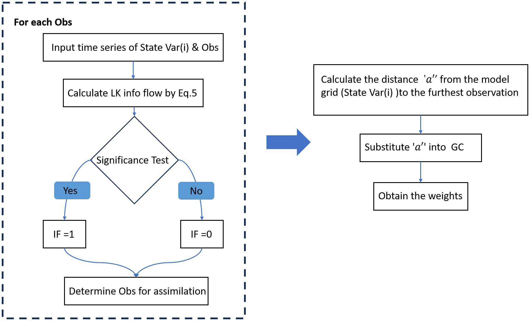
LK information flow-based localization method for single ‘state variable (i)’.
where , represents the information flow from the observation to the jth model grid, which can be treated as a binary filter.
The LK information flow is utilized in the SCDA to not only identify the localization range but also quantify the maximum distance ‘a’ where a causal link is formed. Through the integration with G-C function, a non-empirical localization range that inherently reflects causality can be identified based on information flow analysis, and the corresponding adjusting parameter ‘a’can provide adaptive weights based on the G-C function.
3 Numerical model and twin experiment
3.1 Intermediate atmosphere-ocean-land coupled model
The intermediate atmosphere-ocean-land coupled model (Wu et al., 2012) utilized in this study comprises three main components: a global spectral barotropic atmospheric model, a 1.5-layer baroclinic ocean model, and a simplified land model. These components are interconnected through a specific coupling method designed to simulate the interactions among the atmosphere, ocean, and land. All three model components adopt 64 × 54 Gaussian grid.
The atmospheric component is represented by a global spectral barotropic model as shown in Equation 7, which employs the potential vorticity conservation equation, while accounting for the nonlinear effects of vorticity advection.
where , , f denotes the Coriolis parameter, y represents the northward meridional distance from the equator, represents the Jacobian operator, ψ represents the geostrophic atmosphere stream-function, λ is the flux coefficient from the ocean (land) to the atmosphere, To and Tl denote sea surface temperature (SST) and land surface temperature (LST) respectively, and μ is a scale factor that converts stream-function to temperature.
The ocean is represented by a 1.5-layer baroclinic ocean model shown in Equation 8, which incorporates a slab mixed layer and simulates upwelling through a stream-function equation.
where is the oceanic stream-function, is the oceanic deformation radius, is the reduced gravity and is the mean thermocline depth, is the momentum coupling coefficient between the atmosphere and the ocean, is the horizontal diffusion coefficient of the oceanic stream-function, and are the damping and horizontal diffusion coefficients of sea surface temperature (SST), respectively, represents the intensity of upwelling, is the ratio of upwelling to damping, Co is the flux coefficient from the atmosphere to the ocean is the solar radiation forcing that introduces the seasonal cycle.
The land is modeled using a simple linear approach that simulates the evolution of land surface temperature as illustrated in Equation 9.
where m represents the ratio of heat capacity between the land and the ocean mixed layer, and are damping and diffusive coefficients, respectively, and Cl denotes the flux coefficient from the atmosphere to the land.
The atmospheric model is coupled with the ocean model through flux terms that represent exchanges at both oceanic and terrestrial surfaces. These flux terms are integrated into the potential vorticity conservation equation. The ocean model provides feedback to the atmospheric model via its stream-function equation and heat flux terms, which characterize energy and momentum exchanges between the ocean and the atmosphere. Furthermore, the ocean model is coupled with the land model through heat flux terms that describe energy exchange between the ocean and the land. The land model, represented by a simple linear equation, simulates the evolution of land surface temperature and incorporates feedback from the land surface to the atmospheric model by accounting for heat exchange between the atmosphere and the land surface. All three model components-the atmosphere, ocean, and land-utilize the same 64 × 54 Gaussian grid and are solved using the Leapfrog time integration method with a half-hour time step. An Asselin-Robert time filter is introduced to suppress spurious computational modes that arise from the Leapfrog time integration. Additional information regarding the coupled model, including default parameter settings, can be found in Wu et al. (2012).
3.2 The twin experiment design
To validate the effectiveness of the proposed method, we conducted twin experiments to ensure experimental stability and mitigate performance evaluation errors arising from uncontrolled data uncertainty.
The true model is first created to serve as the baseline system and then used to generate a biased version and an observation system. This true model is initialized with climatological averages , and executes a 55-year integration, with the first 50 years serving as spin-up and the final 5-year outputs constituting the true value. To evaluate the assimilation performance, parameter biases (1.1 times the true values) are introduced to establish the biased model. The model’s outputs provide the prior estimates for subsequent analysis. In this configuration, the systematic errors arise from perturbations in model parameters. Same as the true model, the biased model is also initialized with , and executes a 50-year integration as spin-up. Following previous studies (Wu et al., 2012; Cao et al., 2024), Gaussian white noise with a standard deviation of 106 for ψ, 102 for φ and 1 K for To, and Tl is added as observation errors on the 64×54 Gaussian grid to generate ‘observations’ (Figure 2), where these error magnitudes are set to 4% of the global mean natural variability. The sampling frequencies are 6 hour for and 1 day for φ, To, and Tl fields, due to distinct temporal scale of different components.
Figure 2
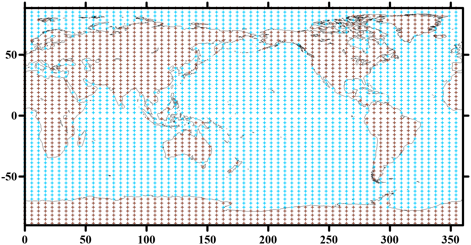
Location of observations, φ/To (blue “+”), Tl (brown “+”), ψ (all “+”).
In this experimental framework, the EAKF is employed to conduct a 5-year state estimation experiment, with the evaluation of results based on the last 5 years of the biased model. As summarized in Table 1, the assimilated variables include ψ, φ, To, and Tl. The assimilation processes for ψ, , and To not only leveraged their own respective observations but also integrated cross-component observations from the other two variables. In contrast, the Tl is solely assimilated using its own observations because it is simulated through a relatively simple and semi-independent structure, which results in weak coupling interactions with other components. The biased model is initialized for a 50-year period to generate the biased initial states of . The ensemble initial states of are produced by superimposing a Gaussian white noise (with a standard deviation of 106) on , whileφ, To, and Tl remain unchanged. The inflation method adopts the adaptive inflation algorithm proposed by Anderson (2007). To facilitate a comparison with the localization method based on LK information flow, the optimal local radii in conventional G-C for ψ and Tl are set at 1,500 and 1,000 km, respectively. The optimal local radius for both φ and To is defined as 1,000 km × cos [min (latitude, 60)], following the study outlined according to Cao et al. (2024). The sensitivity of the LK method to ensemble size is evaluated using configurations N = [5, 10, 20, 30, 40], with specific analysis focused on the N=20 case.
Table 1
| State variables | Observations |
|---|---|
| ψ (Atmosphere stream-function) | ψ, φ, and To |
| φ (Oceanic stream-function) | φ, ψ, and To |
| To (Sea surface temperature) | To, ψ, and φ |
| Tl(Land surface temperature) | Tl |
The SCDA schemes.
The proposed LK information flow-based localization method is tested within the twin experiment. To evaluate its effectiveness and assess the differences between causal and correlational effects on assimilation, the assimilation results are compared with those based on the conventional G-C method in SCDA system. Since an optimized localization can accurately reflect the complex relationships between components and enhance the effectiveness of SCDA, the localization results will thus be discussed first in the next section.
4 Results
The localization results estimated using the LK information flow are compared with the optimal localization radius obtained from the G-C method, followed by an analysis of their corresponding SCDA results. For the LK information flow estimation, a time series consisting of 9600 output times is selected to ensure both efficiency and effectiveness. This length is chosen because a time series that is too short may not satisfy the fundamental assumption of ergodicity, potentially leading to inaccurate results, whereas an excessively long time series would increase the consumption of computational resources.
4.1 The localization results
The localization results based on LK information flow in SCDA are calculated using Equation 5. Where is estimated based on the time series from the observation at the point to the state at the point with a significance test conducted. Liang (2008) pointed out that the values of LK information flow in this context are not directly comparable. Therefore, this study focuses solely on the existence of LK information flow.
Since constructing LK information flow-based localization method requires utilizing the area of LK information flow shown in Figure 3, this result was generated before the first DA cycle. In Figure 3, two grid points were selected for demonstration. The first point is located in the tropical Pacific Ocean, a region dominated by El Niño–Southern Oscillation (ENSO) dynamics. The second point resides in the South Pacific, an area influenced by the Antarctic Circumpolar Current (ACC) and prevailing westerlies. While air–sea interactions at both locations exhibit high activity and intrinsic asymmetry, their underlying physical drivers differ significantly. Figure 3a illustrates the existence range of LK information flow from ψ to φ, demonstrating the influence range of ψ on φ. To compare the influence of the same variable on other variables at the same point, the existing range of LK information flow from ψ to To is presented in Figure 3b. This indicates that the influence range of LK information flow calculated from ψ to φ at the same point differs from that calculated from ψ to To. This finding underscores that the influence range of one variable on each of the other variables varies at the same point. The LK information flow effectively captures this variable heterogeneity, highlighting the differing influence ranges of a variable across multiple variables, which is particularly critical in multi-component systems like SCDA.
Figure 3
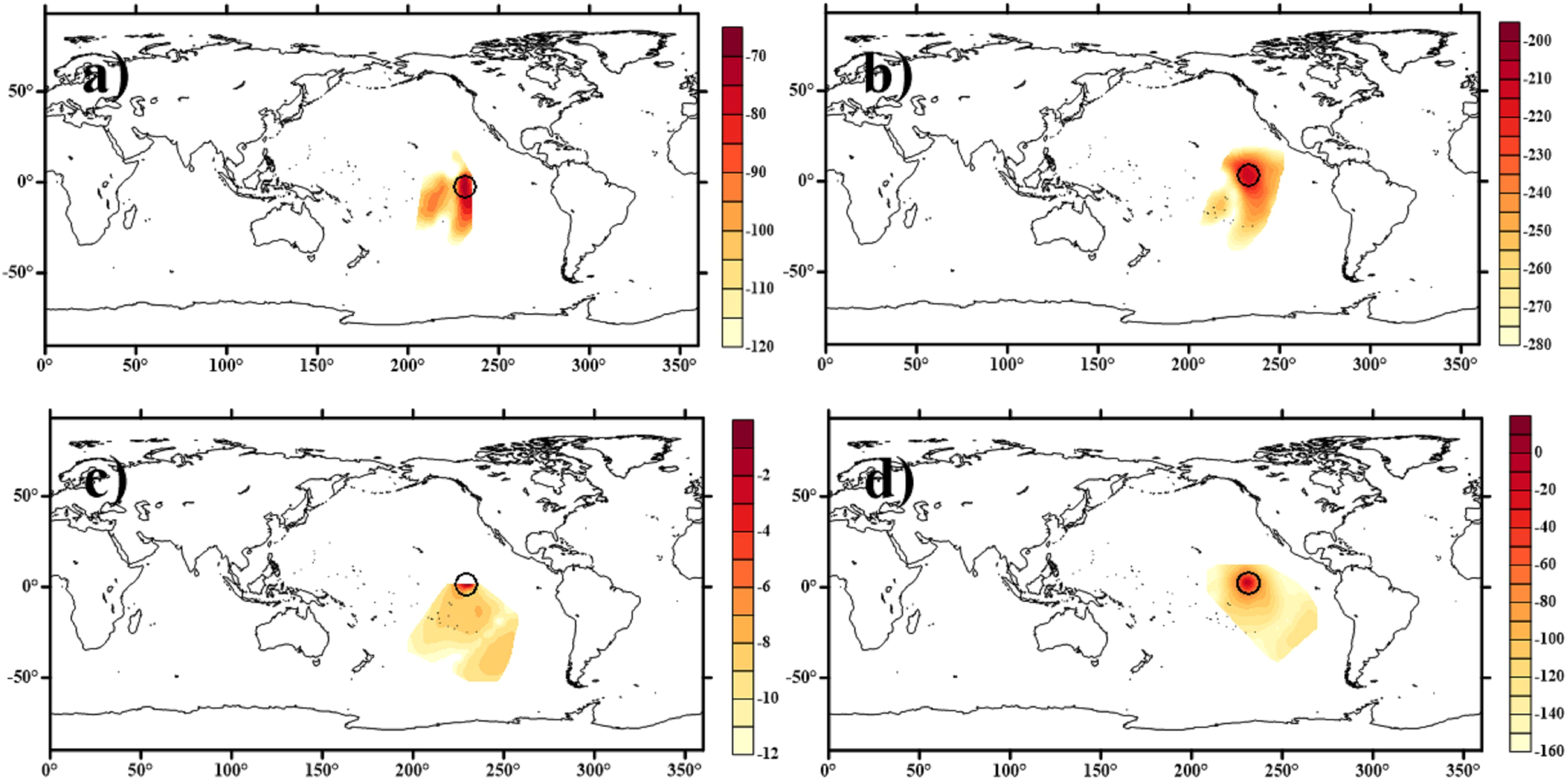
An example of the area and value of LK information flow from (a)ψ (atmosphere stream-function) to φ (oceanic stream-function), (b)ψ to To (sea surface temperature), (c)φ to ψ and (d)To to ψ. Where “○” (black) represents the model grid; The value of LK information in this figure has all undergone logarithmic transformation.
To investigate the directional relationship between the two variables, Figure 3c presents the estimated influence range based on LK information flow from φ to ψ at the same point. In contrast to Figure 3a, the weights between the same variable pair ψ and φ exhibit a distinct pattern and range when considering the inherent causal direction. This observation suggests that even for the same pair of variables, accounting for the directionality of causal interactions reveals asymmetric influence: the ψ at point A may significantly drive the φ at point B, whereas φ at this point of B does not necessarily exert an equivalent influence on ψ at A. If their influences were symmetric, Figures 3a and c would depict identical influence ranges—a phenomenon that is rarely observed in practice. This directional asymmetry is often overlooked by conventional correlation analysis, which assumes relationships to be undirected and homogeneous. The same finding can also be observed in Figure 3d, which illustrates the area and value of LK information flow from To (sea surface temperature) to ψ (atmosphere stream-function) at the same grid point as in Figure 3b.
To investigate whether the relationship between the same two variables exhibits different variations across different points, Figure 2 in supplementary plots the influence range estimated based on LK information flow from ψ to φ at another point. It shows that the ranges to which ψ at two distinct points influence φ are drastically different. This indicates that the intrinsic relationship between variables manifests uniquely at each point, exhibiting spatial heterogeneity. This spatial heterogeneity underscores the unique advantages of causal analysis.
As demonstrated by the results, the relationship between the two components exhibits variable heterogeneity, directional asymmetry, and spatial heterogeneity—characteristics clearly identified and analyzed through the LK information flow. This demonstrates the strengths of causal analysis. Through a comprehensive analysis of these relationships among components, we facilitate an accurate estimation of the cross-component localization parameter, which plays a crucial role in SCDA.
Based on the analysis of the causality between two components, the observational information at a specific point can affect certain aspects of the surrounding model state field. Considering its application in the DA process for coupled systems, the localization area and weights can be estimated based on the range and corresponding magnitude of observations that influence the update of a state variable at a computational grid point as calculated according to Equation 6.
As with Figure 3, the two representative grid points shown in Figure 4 are respectively situated in the ENSO-dominated tropical Pacific Ocean, and the South Pacific region modulated by the ACC and prevailing westerlies. Figure 4b illustrates the influence range and corresponding weights from the observation of ψ to the state variable To at this point, indicating the localization range for the state variable. For comparison, the same localization results based on G-C estimation at the same grid point are presented in Figure 4a. As shown, the localization area in Figure 4a appears as a region with a fixed radius. The G-C method determines the optimal localization radius through empirical trials. In contrast, the localization results estimated by LK information flow exhibit irregular variation (non-isotropic). This indicates a discrepancy between the areas estimated by the two methods. This means that in the assimilation process to update the ψ at the target point, observations of To at certain points, although utilized based on the G-C localization, are actually not used according to LK information flow analysis. Because, according to the judgment of LK information flow, the observations from these points are not deemed to have a direct relationship with the ψ at the target point, and therefore cannot be employed to update the state variables at this location. Moreover, some observations, despite being distant and outside the optimal localization radius of the G-C, are used to update the states at the target point due to their direct causality with the variables requiring updates.
Figure 4
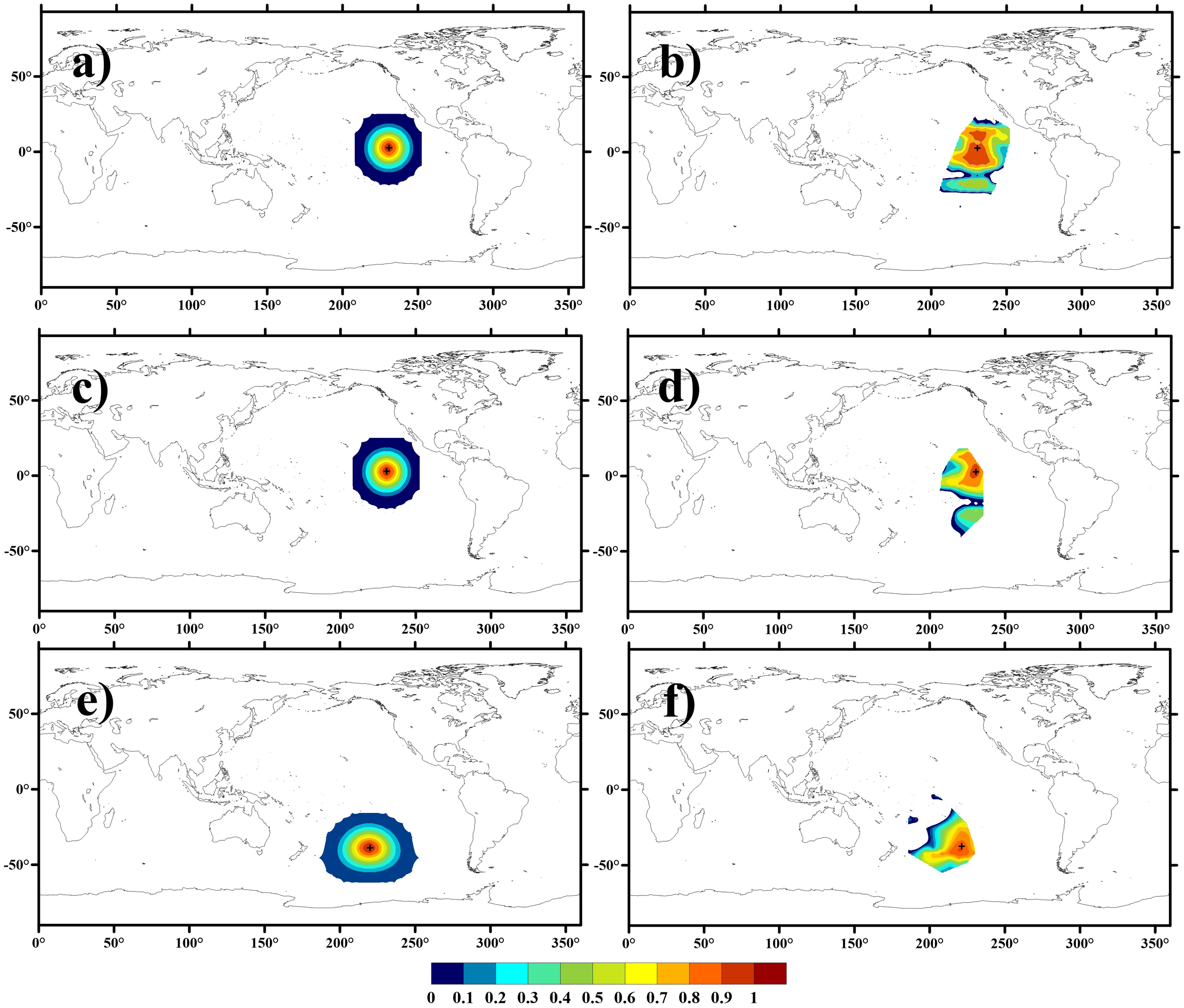
An example of the localization based on the G-C method (a, c, e) and LK information flow-based localization method (b, d, f), which use the observation of ψ (atmosphere stream-function) to update state variables To (sea surface temperature) (a, b) and φ (oceanic stream-function) (c–f). Where “+” (black) represents the location of the state variable, (a–d) are the same model grid point, while (e, f) are another grid point.
Similar findings can be observed between Figures 4c and d, where the localization results for the observation of ψ used to update the state variable φ at the same point are presented. Notably, for the same observation information of ψ, when the state variables that require updating at this computational grid point change, the corresponding localization range and weights also vary. This further indicates that, when updating state variables at a specific point, the observation area required for assimilation is not necessarily identical for different state variables based on the same observed information. In other words, each state variable in the assimilation process, even when located at the same computational grid point, necessitates distinct regions and weights of observational information, reflecting the uniqueness of the variable. This uniqueness is challenging to capture using the G-C method. Conversely, the LK information flow-based localization method effectively distinguishes the varying degrees of influence that the same observation exerts on different state variables. This capability is particularly crucial for coupled systems, such as atmosphere-ocean-land models.
In comparison with Figures 4c and d, the impact of the observation ψ on updating the state variable φ at another computational grid is illustrated in Figures 4e and f. The results of the LK information flow analysis indicate that when identical observations are employed to update the same state variable, both the range of required observations and their corresponding weights vary according to changes in the computational grid points. This finding suggests that the LK information flow-based localization method effectively differentiates the magnitude of influence exerted by observation data on the state variable at various locations. Such spatial heterogeneity may reflect the distinct localized physical environments and dynamic mechanisms surrounding each grid point, which cannot be captured by the G-C method that enforces uniform influence patterns across all grid points.
Overall, when updating a state variable, the LK information flow method, in contrast to the G-C method which assumes isotropic relationships between state variables and surrounding observations, can identify and select the relevant range and weight of correlated observations for each state variable at each computational grid. As noted by Gaspari and Cohn (1999), the correlations of geophysical fields rarely exhibit such special symmetries. Thus, this anisotropy may align more closely with physical laws and contribute to the advancement of SCDA.
4.2 Assimilation results with 20 ensembles
Based on the aforementioned localization estimation, the SCDA was conducted, and the results were statistically assessed using the spatially averaged root mean square error () as defined in Equation 10, and the temporally averaged root mean square error () over the last year, as defined in Equation 11.
where I and J represent the number of rows and columns, respectively, within the model grid, and represent the ensemble mean of the variables and true value at the (i,j) grid point at time s, respectively.
where S represents the number of time steps.
The spatially averaged RMSE at each time step obtained from the twin experiment based on localization of the LK information flow localization method is depicted as the orange line in Figure 5. Figures 5a–d illustrate the assimilation results for ψ, φ, To, and Tl, respectively. For comparison, the DA results based on G-C localization are represented in the blue line. It can be observed that the assimilation results based on G-C localization stabilize at approximately 0.8 to 1 year. In contrast, when considering the LK information flow for localization, the updated ψ, φ, and To align more closely with the true values, with the presented error decreasing within half a year. Notably, for ψ, the assimilated result based on the localization of LK information flow exhibits an error of 2.36×10⁵, which is 5% lower than that obtained through G-C localization. In the case of To, the error is further suppressed to 0.28 K, a 22% reduction relative to the G-C. φ exhibits the most pronounced enhancement: its error decreases from 61 under G-C localization to 29 with the LK method, achieving a 51% improvement. Regarding the assimilation results for Tl shown in Figure 5d, both experiments yield consistent outcomes. As indicated in Table 1, it is important to note that the state variable Tl is updated solely by assimilating observations of Tl itself. Since only the information from a single observed element is considered in relation to the corresponding state variable at the assimilated grid point. Consequently, the influence of surrounding observed information on the assimilated point is likely to exhibit a homogeneous variation concerning distance. Therefore, the two localization methods are likely to yield similar results in estimating their relationship, thus resulting in no significant differences in the assimilation outcomes.
Figure 5
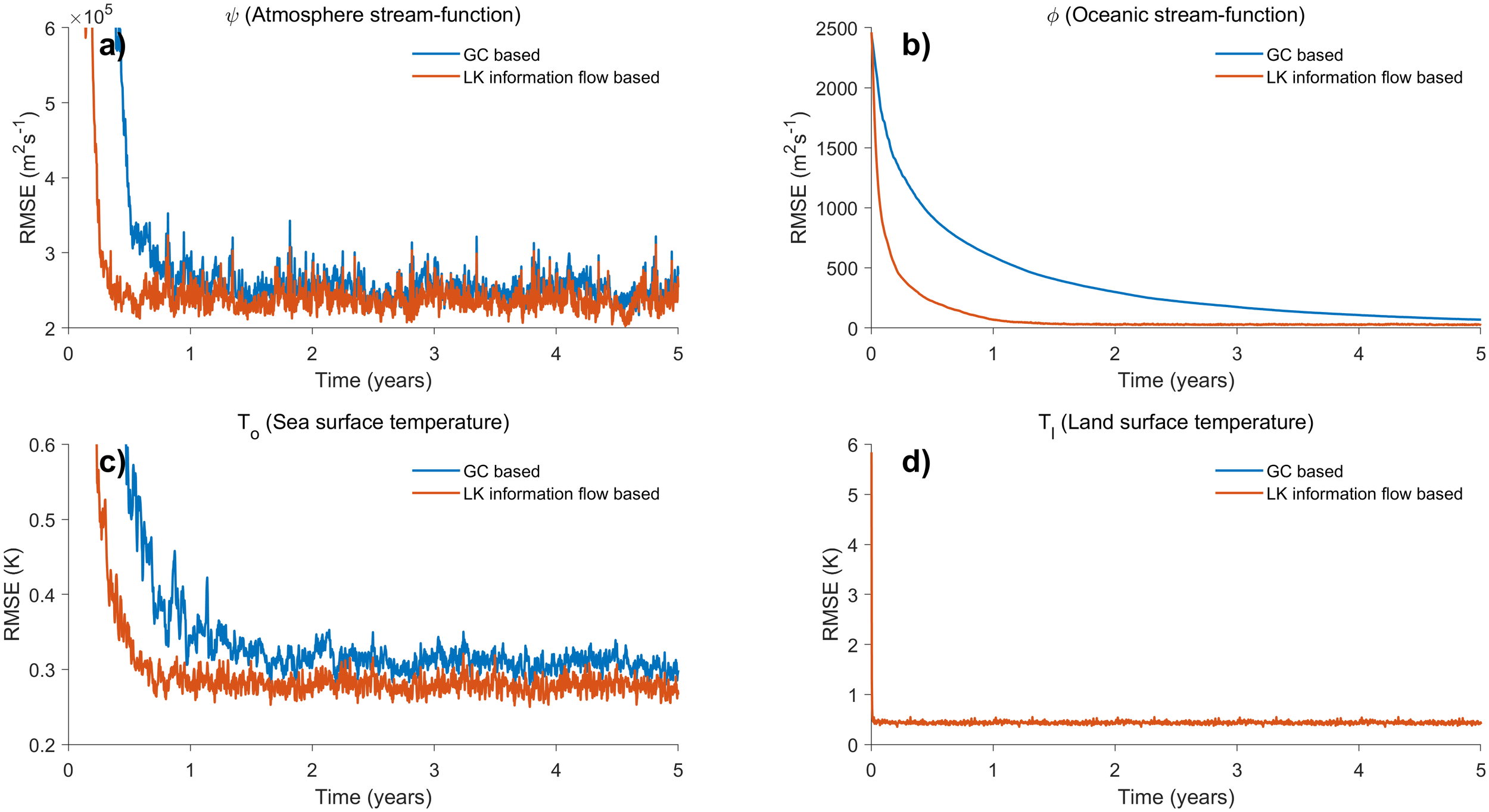
Spatially averaged RMSE time series based on LK information flow-based localization method and G-C method. Variables shown are the (a)ψ (atmosphere stream-function, ), (b) φ (oceanic stream-function, ), (c)To (sea surface temperature, K) and (d)Tl (land surface temperature, K).
Overall, the observational information required for updating each computational grid is typically inhomogeneous, both spatially and in relation to specific variables, particularly when transferring information across components. Consequently, the LK information flow-based SCDA demonstrates faster stabilization and more convincing performance.
To further illustrate the spatial variation of the assimilation results, the RMSE averaged over the final year after the system reaches a stable state is analyzed for the SCDA based on LK information methods for ψ, φ, and To are shown in Figures 6a, c and e, respectively. As observed, the assimilated RMSE for ψ exhibits higher values in land areas depicted in Figure 6a. Figure 6c illustrates that the errors in the assimilation results for demonstrate a decreasing trend from the equator to the poles. In contrast, the RMSE of the assimilation results for To is more evenly distributed globally. The spatial error patterns in the assimilation results stem from the biased model used in this study. Specifically, parameter perturbations introduced systematic biases, which vary across variables and regions due to their differential sensitivity to parameters (Wu et al., 2012). Furthermore, the geographical sensitivity of the parameters leads to different magnitudes of bias for the same variable across different regions. As a systematic bias caused by parameter perturbations, it can only be corrected through parameter optimization. The characteristics of the distributions presented in the three plots of our experimental results are caused by systematic bias and do not fall within the scope of correction in this state field estimation test. Therefore, it is more valuable to focus on the error differences in the assimilation results compared to another G-C-based localization method.
Figure 6
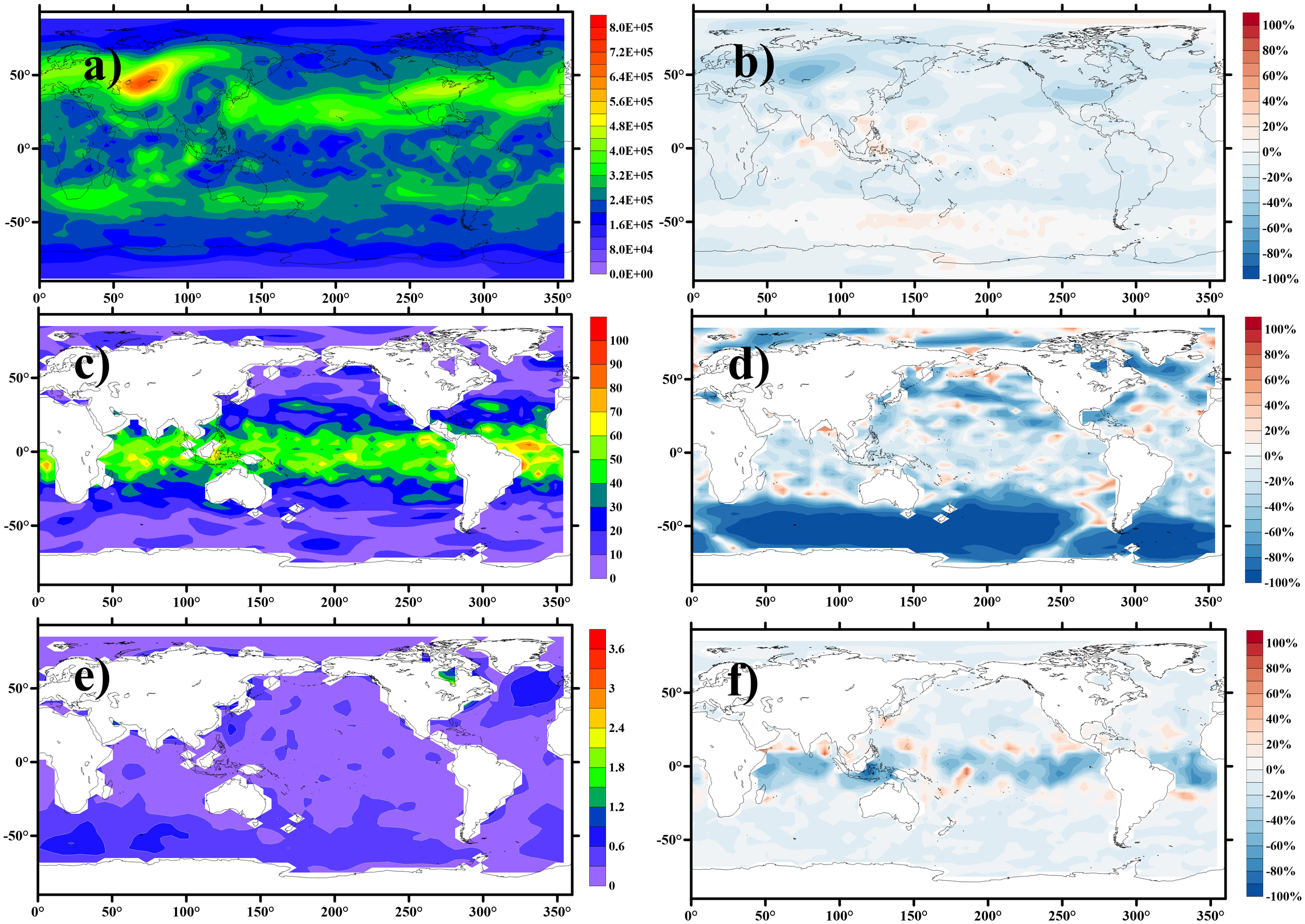
Temporally averaged RMSE (the final year) based on LK information flow-based localization method (a, c, e) and the percentage error reduction achieved by the LK localization relative to the G-C method, calculated as (e_LK – e_GC)/e_GC × 100% (b, d, f). Variables shown are the (a, b)ψ (atmosphere stream-function, ), (c, d)φ (oceanic stream-function, ), (e, f)To (sea surface temperature, K).
The percentage error reduction achieved by the LK localization relative to the G-C method (calculated as (e_LK – e_GC)/e_GC × 100%) is illustrated in Figures 6b, d and f. It is evident that the assimilation results derived from the LK information flow method exhibit a significant reduction in error across this simulation region when compared to those obtained from the G-C method. This finding suggests that the LK information flow-based localization method enhances the assimilation results, both under high-resolution observational data in the polar regions and low-resolution observational data in the equatorial region, thereby demonstrating the universality of the LK method. Notably, the assimilation results for φ reveal a substantial decrease in error in the Southern Ocean region following localization via the LK information flow. This outcome indicates that the LK information flow analysis effectively filters out spurious correlations between φ and other components in this region while preserving the fundamental coupling mechanisms and integrating causally related observational information into the assimilation process, resulting in a marked improvement in assimilation effectiveness.
4.3 Ensemble size sensitivity test
Robustness evaluation of the LK localization method across ensemble size variations was conducted via dedicated sensitivity analysis, systematically testing configurations encompassing N = [5, 10, 20, 30, 40]. The results were statistically assessed using the spatial-temporal average and associated standard deviation over the last year, as defined in Equations 12 and 13.
Where, represents spatially averaged RMSE, as defined in Equation 10; represents the standard deviation.
The result of the ensemble size sensitivity test is shown in Figure 7. Figures 7a–c respectively display the Spatial-temporal average and associated standard deviations for variables ψ, φ, and To using both localization methods across multiple ensemble sizes. It is observed that errors for all variables decrease with increasing ensemble size under both localization schemes. The G-C method exhibits greater sensitivity to ensemble size than the LK method, demonstrating a more rapid error reduction. This occurs because larger ensembles effectively mitigate the impact of spurious correlations. However, the intrinsic ability of the LK method to suppress spurious correlations attenuates the error-reducing effect of increased ensemble size. Notably, even at larger ensemble sizes, the G-C method yields higher errors than the LK method at equivalent ensemble sizes, though the performance gap between the two methods narrows as the ensemble size increases. Crucially, filter divergence occurs when using the G-C method at an ensemble size of 5, while the LK method maintains stability—albeit with larger errors. This indicates that although the LK method effectively reduces errors for small ensemble sizes, its capability to suppress spurious correlations is significantly diminished under extremely small ensembles (e.g., N=5) due to severely limited information availability.
Figure 7
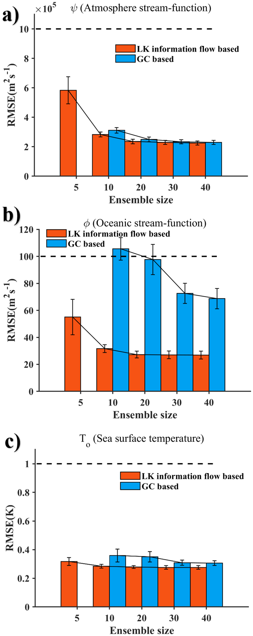
Spatial-temporal average and standard deviation of last 1 year based on G-C and LK method. Variables shown are the (a)ψ (atmosphere stream-function, ), (b) φ (oceanic stream-function, ), (c)To (sea surface temperature, K).
5 Discussion
Prior studies have highlighted both the significance and the challenges associated with implementing SCDA. In this study, we seek to diagnose and identify the inherent relationships between two components to adjust the assimilation process in a coupled system. The LK information flow analysis was employed to assess relationships not only among various variables but also between observation and state variables, as well as information across different geographic locations. One interesting finding is that different state variables respond to observed information in distinct and directional ways. Additionally, the effect of observational information on a state variable is characterized differently across geographic locations. These insights are revealed through causality analysis using the LK information flow method, which offers capabilities beyond conventional G-C optimization based on correlation analysis. Critically, ensemble size sensitivity tests demonstrate that the LK method’s advantages are particularly pronounced in small ensembles (e.g., ensemble size of 5, 10, and 20). When the G-C method optimizes the influence radius of observational information, it assumes isotropic among internal components, often neglecting variable–specific directional couplings and scale disparities between components (as shown in Figure 3). In contrast, the LK method not only utilizes observations beyond the empirical radius defined by the G-C method but also eliminates non-causal statistical noise within the G-C optimized range, thereby avoiding filter divergence observed in G-C at N=5 (Figure 7) and resulting in LK method-based SCDA stabilizing more quickly and achieving greater accuracy.
These findings further confirm that one factor limiting the improvement of SCDA performance is its high sensitivity to hyperparameters, such as localization (Miwa and Sawada, 2024). Specifically, when the ensemble size is small, SCDA’s performance becomes more vulnerable to variations in hyperparameters. This highlights the practical necessity of accurately estimating SCDA’s hyperparameters to ensure better performance. Grounded in causal analysis theory, the LK method reframes the empirical determination of localization parameters as a quantitative assessment of causal dependence strength. This establishes a physically constrained framework for determining localization parameters, thereby enhancing the robustness of SCDA.
Our study was conducted based on twin experiments of an ideal model. Further research is needed to determine whether the LK method can be extended to real-world assimilation systems. In practice, for coupled assimilation systems, the primary challenges arise from the larger number of components that must be managed, the stronger nonlinear characteristics, and the more irregularity of observational information. The LK method’s ability to identify causality among components is particularly advantageous for filtering out consistent information in complex coupled systems, thereby avoiding interference among components. Regarding the irregular features that may exist in observational data, such as resolution or uncertainty, the LK method requires only the time series from the observation positions with no specific resolution requirements. Noisy observations can also be screened and eliminated. Furthermore, earlier studies have shown that LK information flow maintains its capacity to accurately determine causality even within highly nonlinear systems (Liang, 2014) and demonstrates strong robustness in high-noise environments (Zhou et al., 2024). Therefore, we believe that the application of LK information-based SCDA will also show stable and convincing performance in practical trials.
6 Conclusions
This study proposes a causality-driven adaptive localization method, termed the LK information flow localization method, aimed at enhancing SCDA by addressing critical challenges such as sensitivity to hyperparameters and spurious correlations in cross-component interactions. By leveraging causality analysis, the LK method offers a physically constrained framework for localization, facilitating more accurate and efficient assimilation of observational data across coupled systems. By integrating the LK information flow with the EAKF within an intermediate atmosphere–ocean–land coupled model, our results reveal that the LK-based SCDA effectively captures variable heterogeneity, directional asymmetry, and spatial heterogeneity in component interactions, which are often overlooked by conventional correlation-based methods like conventional G-C localization. These capabilities enable the LK method to filter out non-causal statistical noise and utilize observations beyond the empirical radius of G-C, resulting in faster stabilization and significantly improved assimilation accuracy.
While the LK method exhibits distinct advantages in small-ensemble regimes due to its causality analysis, its capability to achieve high absolute accuracy is still limited by the small ensemble size. Specifically, the errors (e.g., RMSE) obtained with the LK method using small ensembles are smaller than those of the G-C method, but their absolute errors remain considerable. Moreover, ensemble sensitivity tests confirm that the performance gap between LK and G-C narrows rapidly beyond a threshold, with diminishing returns on LK’s relative improvement as ensemble size increases. This convergence indicates that LK’s distinctive value may diminish in computational environments supporting larger ensembles, where G-C’s isotropic localization benefits more directly from inflated sampling. Although the computation of information flow can be parallelized, the additional computational cost incurred under high-resolution operating systems remains non-negligible. When the LK method demonstrates comparable errors to the G-C method under large-ensemble conditions, a trade-off between computational cost and accuracy must be carefully considered.
The twin experiments conducted in this study highlight the potential of the LK method to enhance SCDA performance, particularly in systems characterized by small ensemble sizes and complex interactions. However, the current work focuses on the stable, large-scale dynamics between coupled components. The performance of this static framework in capturing real-world transient, small-scale dynamics remains to be validated. In addition, future work should also explore the integration of flow-dependent ensemble covariances within the LK framework to define the information flow dynamically throughout the DA window. Such development would allow the information pathways to adapt instantaneously to the evolving atmospheric and oceanic states, potentially capturing fast-changing interactions between the two components more accurately. This dynamic framework could also be applied to vertical localization. However, given that observation devices below the sea surface are often mobile, obtaining long-term measurements at a fixed position becomes challenging. In such scenarios, how to implement the LK method will be a key focus of our future work. Notwithstanding these challenges, the LK method establishes a new approach to localization by replacing empirical parameterization with causality, thereby positioning it to enhance the accuracy and reliability of Earth system predictions.
Statements
Data availability statement
The original contributions presented in the study are included in the article/Supplementary Material. Further inquiries can be directed to the corresponding author.
Author contributions
TW: Writing – original draft, Writing – review & editing. XW: Writing – review & editing. LC: Writing – review & editing. WL: Writing – review & editing. GH: Writing – review & editing.
Funding
The author(s) declare financial support was received for the research and/or publication of this article. This research is cosponsored by grants from the National Key Research and Development Program of China(2023YFC3107802).
Acknowledgments
We would like to express our sincere gratitude to Professor X S Liang for providing the valuable method and sincerely appreciate the editor and reviewers for their valuable comments and suggestions that helped us improve the quality of the article.
Conflict of interest
The authors declare that the research was conducted in the absence of any commercial or financial relationships that could be construed as a potential conflict of interest.
Generative AI statement
The author(s) declare that no Generative AI was used in the creation of this manuscript.
Any alternative text (alt text) provided alongside figures in this article has been generated by Frontiers with the support of artificial intelligence and reasonable efforts have been made to ensure accuracy, including review by the authors wherever possible. If you identify any issues, please contact us.
Publisher’s note
All claims expressed in this article are solely those of the authors and do not necessarily represent those of their affiliated organizations, or those of the publisher, the editors and the reviewers. Any product that may be evaluated in this article, or claim that may be made by its manufacturer, is not guaranteed or endorsed by the publisher.
Supplementary material
The Supplementary Material for this article can be found online at: https://www.frontiersin.org/articles/10.3389/fmars.2025.1600634/full#supplementary-material
References
1
Anderson J. L. (2001). An ensemble adjustment kalman filter for data assimilation. Monthly Weather Rev.129, 2884–2903. doi: 10.1175/1520-0493(2001)129<2884:AEAKFF>2.0.CO;2
2
Anderson J. L. (2003). A local least squares framework for ensemble filtering. Monthly Weather Rev.131, 634–642. doi: 10.1175/1520-0493(2003)131<0634:ALLSFF>2.0.CO;2
3
Anderson J. L. (2007). Exploring the need for localization in ensemble data assimilation using a hierarchical ensemble filter. Physica D: Nonlinear Phenomena230, 99–111. doi: 10.1016/j.physd.2006.02.011
4
Anderson J. Lei L. (2013). Empirical localization of observation impact in ensemble kalman filters. Monthly Weather Rev.141, 4140–4153. doi: 10.1175/MWR-D-12-00330.1
5
Burgers G. Leeuwen P.J.v. Evensen G. (1998). Analysis scheme in the ensemble kalman filter. Monthly Weather Rev.126, 1719–1724. doi: 10.1175/1520-0493(1998)126<1719:ASITEK>2.0.CO;2
6
Cao L. Han G. Li W. Wu H. Wu X. Zhou G. et al . (2024). Impact of instantaneous parameter sensitivity on ensemble-based parameter estimation: simulation with an intermediate coupled model. J. Adv. Modeling Earth Syst.16, e2024MS004253. doi: 10.1029/2024MS004253
7
Chang C.-C. Kalnay E. (2022). Applying prior correlations for ensemble-based spatial localization. Nonlinear Processes Geophysics29, 317–327. doi: 10.5194/npg-29-317-2022
8
Evensen G. (1994). Sequential data assimilation with a nonlinear quasi-geostrophic model using Monte Carlo methods to forecast error statistics. J. Geophysical Research: Oceans99, 10143–10162. doi: 10.1029/94JC00572
9
Evensen G. (1997). Advanced data assimilation for strongly nonlinear dynamics. Monthly Weather Rev.125, 1342–1354. doi: 10.1175/1520-0493(1997)125<1342:ADAFSN>2.0.CO;2
10
Frolov S. Rousseaux C. S. Auligne T. Dee D. Gelaro R. Heimbach P. et al . (2023). Road map for the next decade of earth system reanalysis in the United States. Bull. Am. Meteorological Soc.104, E706–E714. doi: 10.1175/BAMS-D-23-0011.1
11
Gaspari G. Cohn S. E. (1999). Construction of correlation functions in two and three dimensions. Q. J. R. Meteorological Soc.125, 723–757. doi: 10.1002/qj.49712555417
12
Goodliff M. Penny S. G. (2022). Developing 4D-var for strongly coupled data assimilation using a coupled atmosphere–ocean quasigeostrophic model. Monthly Weather Rev.150, 2443–2458. doi: 10.1175/MWR-D-21-0240.1
13
Hagan D. F. T. Wang G. Liang X. S. Dolman H. A. J. (2019). A time-varying causality formalism based on the Liang-Kleeman information flow for analyzing directed interactions in nonstationary climate systems. J. Climate32, 7521–7537. doi: 10.1175/JCLI-D-18-0881.1
14
Han G. Wu X. Zhang S. Liu Z. Li W. (2013). Error covariance estimation for coupled data assimilation using a lorenz atmosphere and a simple pycnocline ocean model. J. Climate26, 10218–10231. doi: 10.1175/JCLI-D-13-00236.1
15
Houtekamer P. L. Mitchell H. L. (1998). Data assimilation using an ensemble kalman filter technique. Monthly Weather Rev.126, 796–811. doi: 10.1175/1520-0493(1998)126<0796:DAUAEK>2.0.CO;2
16
Houtekamer P. L. Mitchell H. L. Pellerin G. Buehner M. Charron M. Spacek L. et al . (2005). Atmospheric data assimilation with an ensemble kalman filter: results with real observations. Monthly Weather Rev.133, 604–620. doi: 10.1175/MWR-2864.1
17
Houtekamer P. L. Zhang F. (2016). Review of the ensemble kalman filter for atmospheric data assimilation. Monthly Weather Rev.144, 4489–4532. doi: 10.1175/MWR-D-15-0440.1
18
Lei L. Anderson J. L. (2014a). Comparisons of empirical localization techniques for serial ensemble kalman filters in a simple atmospheric general circulation model. Monthly Weather Rev.142, 739–754. doi: 10.1175/MWR-D-13-00152.1
19
Lei L. Anderson J. L. (2014b). Empirical localization of observations for serial ensemble kalman filter data assimilation in an atmospheric general circulation model. Monthly Weather Rev.142, 1835–1851. doi: 10.1175/MWR-D-13-00288.1
20
Liang X. S. (2008). Information flow within stochastic dynamical systems. Phys. Rev. E78, 31113. doi: 10.1103/PhysRevE.78.031113
21
Liang X. S. (2014). Unraveling the cause-effect relation between time series. Phys. Rev. E90, 52150. doi: 10.1103/PhysRevE.90.052150
22
Liang X. S. Kleeman R. (2005). Information transfer between dynamical system components. Phys. Rev. Lett.95, 244101. doi: 10.1103/PhysRevLett.95.244101
23
Liang X. S. Xu F. Rong Y. Zhang R. Tang X. Zhang F. (2021). El Niño Modoki can be mostly predicted more than 10 years ahead of time. Sci. Rep.11, 17860. doi: 10.1038/s41598-021-97111-y
24
Lu F. Liu Z. Zhang S. Liu Y. Jacob R. (2015). Strongly coupled data assimilation using leading averaged coupled covariance (LACC). Part II: CG-CM experiments. Monthly Weather Rev.143, 4645–4659. doi: 10.1175/MWR-D-15-0088.1
25
Lu X. Sun J. Wei G. Chang C.-T. (2023). Causal interactions and financial contagion among the BRICS stock markets under rare events: A Liang causality analysis. Int. J. Emerging Markets20, 2014–2041. doi: 10.1108/IJOEM-01-2023-0055
26
Miwa N. Sawada Y. (2024). Strongly versus weakly coupled data assimilation in coupled systems with various inter-compartment interactions. J. Adv. Modeling Earth Syst.16, e2022MS003113. doi: 10.1029/2022MS003113
27
Pearl J. Mackenzie D. (2018). The book of why: The new science of cause and effect. Science361, 855–855. doi: 10.1126/science.aau9731
28
Penny S. G. Bach E. Bhargava K. Chang C.-C. Da C. Sun L. et al . (2019). Strongly coupled data assimilation in multiscale media: experiments using a quasi-geostrophic coupled model. J. Adv. Modeling Earth Syst.11, 1803–1829. doi: 10.1029/2019MS001652
29
Rong Y. Liang X. S. (2022). An information flow-based sea surface height reconstruction through machine learning. IEEE Trans. Geosci. Remote Sens.60, 1–9. doi: 10.1109/TGRS.2022.3140398
30
Sluka T. C. Penny S. G. Kalnay E. Miyoshi T. (2016). Assimilating atmospheric observations into the ocean using strongly coupled ensemble data assimilation. Geophysical Res. Lett.43, 752–759. doi: 10.1002/2015GL067238
31
Stanley Z. C. Draper C. Frolov S. Slivinski L. C. Huang W. Winterbottom H. R. (2024). Vertical localization for strongly coupled data assimilation: experiments in a global coupled atmosphere-ocean model. J. Adv. Modeling Earth Syst.16, e2023MS003783. doi: 10.1029/2023MS003783
32
Stips A. Macias D. Coughlan C. Garcia-Gorriz E. Liang X. S. (2016). On the causal structure between CO2 and global temperature. Sci. Rep.6, 21691. doi: 10.1038/srep21691
33
Wu X. Zhang S. Liu Z. Rosati A. Delworth T. L. Liu Y. (2012). Impact of geographic-dependent parameter optimization on climate estimation and prediction: simulation with an intermediate coupled model. Monthly Weather Rev.140, 3956–3971. doi: 10.1175/MWR-D-11-00298.1
34
Yoshida T. Kalnay E. (2018). Correlation-cutoff method for covariance localization in strongly coupled data assimilation. Monthly Weather Rev.146, 2881–2889. doi: 10.1175/MWR-D-17-0365.1
35
Zhou D. Liu J. Yang X. Wei Y. Wu Z. Li M. (2024). “The bayesian network method for handling cyclic loops based on information flow,” in 2024 IEEE 6th International Conference on Civil Aviation Safety and Information Technology (ICCASIT). 789–793. doi: 10.1109/ICCASIT62299.2024.10827953
Summary
Keywords
strongly coupled data assimilation, EAKF, localization, adaptive method, causal analysis
Citation
Wang T, Wang X, Cao L, Li W and Han G (2025) Causality-driven localization method for improving ensemble-based Kalman filters in strongly coupled data assimilation system. Front. Mar. Sci. 12:1600634. doi: 10.3389/fmars.2025.1600634
Received
26 March 2025
Accepted
07 August 2025
Published
04 September 2025
Volume
12 - 2025
Edited by
Andrea Storto, National Research Council (CNR), Italy
Reviewed by
Lilian Garcia-Oliva, Barcelona Supercomputing Center, Spain
Luyu Sun, University of Maryland, College Park, United States
Kenta Kurosawa, Chiba University, Japan
Updates
Copyright
© 2025 Wang, Wang, Cao, Li and Han.
This is an open-access article distributed under the terms of the Creative Commons Attribution License (CC BY). The use, distribution or reproduction in other forums is permitted, provided the original author(s) and the copyright owner(s) are credited and that the original publication in this journal is cited, in accordance with accepted academic practice. No use, distribution or reproduction is permitted which does not comply with these terms.
*Correspondence: Xuan Wang, xuanwang@tju.edu.cn
Disclaimer
All claims expressed in this article are solely those of the authors and do not necessarily represent those of their affiliated organizations, or those of the publisher, the editors and the reviewers. Any product that may be evaluated in this article or claim that may be made by its manufacturer is not guaranteed or endorsed by the publisher.