The variability of wind-driven currents in the Norwegian Trench

The Norwegian Trench (NT) is the main pathway for North Sea water into the Atlantic Ocean and for Atlantic Water (AW) into the North Sea. The processes that determine the cross-shelf exchange through the NT are key to understanding the variability of the salt budgets in the North Sea. Here, high-resolution numerical simulations from Copernicus Marine Services (CMEMS) for two recent years (2022, 2023) reveal new sources of variability of the flows in the NT. We find that wind regulates the flows in the NT, particularly in enabling the outflow of the fresh-water river plume, the Norwegian Coastal Current (NCC), in the Skagerrak during easterly wind conditions. Strong NCC outflows are associated with transport in a northward direction into the Atlantic Ocean. Furthermore, intensified eddy activity at the surface is found during strong NCC flows, causing high velocity surface currents sometimes exceeding magnitudes of 1 m/s. AW inflows partly compensate the northward outflows, keeping the net transport of 2–3 Sv constant over both years. However, the magnitudes of the AW inflows are small compared to the NCC. AW inflows that are comparable to the NCC outflows only occur during northerly winds in winter. We show that the variability of surface flows in the NT is wind induced, but that the effects of the canyon-like shape of the NT and seasonality of winds and river discharges introduce more variable deep flows than previously considered.

1 Introduction

The North Sea in northern Europe (Figure 1A) is one of the best-studied shelf seas worldwide (Huthnance et al., 2022). Disproportional to its small size, the North Sea is of large ecologic importance (Van Der Molen and Paetsch, 2022; Huthnance et al., 2022). Overall the North Sea is a shallow sea with an average depth of approximately 100 m. However, the Norwegian Trench (NT), a deep canyon along the Norwegian coast, has an average water depth of 300 m (Hovland and Indreeide, 1980). The NT plays a key role in the exchange with the Atlantic Ocean by channelling the outflow of the North Sea waters (Huthnance et al., 2009; Hordoir et al., 2013; Christensen et al., 2018). Davies and Heaps (1980) showed that the NT influences the wind-driven circulation of the North Sea, in particularly in forcing inflows over the shelf into the North Sea as a compensation for intensified outflows through the trench. The NT emerges from the Skagerrak, extends northward coast-parallel to Norway, and ends in the Norwegian Sea (Johannessen et al., 1989). The conceptual overview in Figure 1A is based on previous studies about the NT, e.g. McClimans and Lonseth (1985); Furnes et al. (1986); Sætre et al. (1988); Johannessen et al. (1989) and Hordoir et al. (2013). Mork (1981) summarized first insights about the dynamics in the NT based on the data that was collected during “The Norwegian Coastal current” project, which started in 1975. The Norwegian Coastal Current (NCC) is a baroclinic coastal trapped current composed of fresher waters from the North Sea, the Baltic Current (BC), the Jutland Current (JC) and from the many fjords and rivers, e.g. Glomma, around Norway (Christensen et al., 2018; Skagseth et al., 2011). The water of the NCC is characterized by salinities below 35 PSU, however freshening due to fjord outflows can reduce the salinity below 32 PSU (Johannessen, 1986). The magnitude of the contribution and the principal source of freshwater is spatially and temporally variable, changing along the Norwegian coastline and over the seasonal cycle (Skagseth et al., 2011). Formed in the Skagerrak, the NCC flows northward along the coastline of Norway on the eastern side of the NT. Due to its lower density, the NCC flows in the upper 50–100 m of the water column and stratifies the system (Ikeda et al., 1989; Albretsen et al., 2012). Partly, underneath the NCC the recirculating waters of the North Sea flow northward out of the North Sea into the Atlantic Ocean (Winther and Johannessen, 2006). Outflows of the NCC are related to westerly and easterly wind conditions in the Skagerrak, which result in blocking and outbreak conditions, respectively (Mork, 1981; Christensen et al., 2018; Hordoir et al., 2013). The seasonality in prevailing winds strongly affects the width, depth, and strength of the NCC (Mork, 1981; Sætre et al., 1988). A typical observation is that a branch of the NCC deviates westwards at 58°N, before turning eastwards farther North (Ikeda et al., 1989). Multiple studies observed that intense winds over autumn and winter increase the wind-driven transport of the NCC, whereas over summer when winds weaken, the transport decreases (Davies and Heaps, 1980; Skagseth et al., 2011; Winther and Johannessen, 2006). Along-shore and cross-shore winds can favour upwelling and downwelling conditions, thus widening and shallowing the NCC or deepening and narrowing it, respectively (Davies and Heaps, 1980; Huthnance et al., 2009).

Figure 1

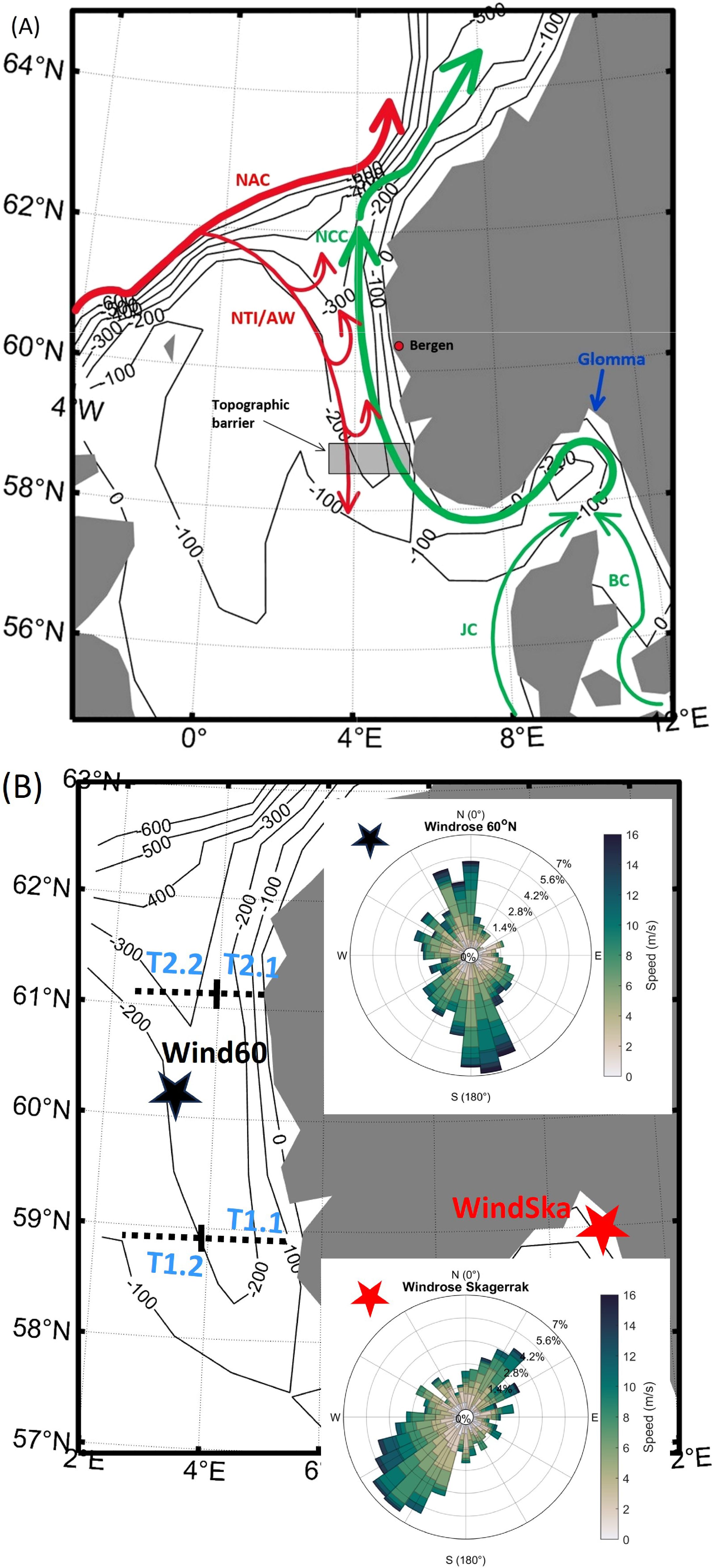
Figure 1. (A) Map of schematized mean currents in the northern North Sea: The Jutland Current (JC) and the Baltic Current (BC) meet in the Skagerrak and form the Norwegian Coastal Current (NCC). The NCC flows alongshore and northwards following the Norwegian coastline. From the north, the Atlantic Water (AW) branching from the North Atlantic Current (NAC) flows southward along the western side into the trench as NT Inflow (NTI). The discharge of the Glomma River contributes to the freshwater body of the NCC. The topographic map generated with MATLABs M_Map package shows bathymetry data in metres (Pawlowicz, 2020). (B) Topographic map showing the study area of the NT, the four transect (T1.1, T1.2, T2.1 and T2.2) and the two locations of the wind time series. The two wind roses show the daily mean wind speeds and directions from 01-01–2022 to 31-12–2023 for wind site 60°N and the Skagerrak. The wind roses display the direction of origin of the wind.

The Atlantic Water (AW) branching from the North Atlantic Current (NAC), flows southwards along the western side of the NT as NT Inflow (NTI), see Winther and Johannessen (2006) and Johannessen et al. (1989). The AW is classified by salinities equal to or higher than 35 PSU (Furnes et al., 1986). As the NAC carries heat from the subtropics, the NTI is warmer than the North Sea waters (Albretsen et al., 2012). In the NT, the currents at higher depth are influenced by the shape of the trench and its topography (Mork, 1981). Approximately, half of the inflowing AW is redirected eastwards at 58.5°N – 59°N and continues northwards underneath the NCC, see Figure 1A (Furnes et al., 1986; Ikeda et al., 1989). Along these latitudes, a steep change in topography acts like a barrier to the AW flow as it restricts the width of the trench and the southward flows through the NT. In previous studies, the eastward redirection of AW, is referred to as retroflection (Furnes et al., 1986). Additionally, southward shoaling causes a deflection of the currents to the east by topographic steering already at higher latitudes (Johannessen et al., 1989; McClimans et al., 2000). AW inflow events that reach farther south into the NT and renew the bottom water are rare and are only observed under very cold winter conditions (Mork, 1981). These AW inflow events are the main source of salinity and heat for the North Sea in winter (Albretsen et al., 2012). Whether these events are wind or density driven is not clear yet.

Within the NT, mesoscale eddies, sharp fronts, and meanders are the result of baroclinic instabilities caused by the interaction of the NCC and the AW (Ikeda et al., 1989; McClimans et al., 2000). On short time scales, eddies can cause flow velocities at the surface that exceed magnitudes of 1 m/s. McClimans et al. (2009) found that surface eddies impact the entire water column and can be measured down to the bed of the NT. Anticyclonic eddies with large baroclinic contributions are present on the eastern side, while cyclonic eddies from barotropic instabilities are found in the northwestern part of the NT (Ikeda et al., 1989; Johannessen et al., 1989). Due to mixing and the lack of sufficient freshwater sources to sustain the low salinity of the NCC, the salinity of the NCC increases northwards (Skagseth et al., 2011). Horizontal and vertical density gradients weaken, such that the generation of eddies is suppressed.

Various studies suggest that the net cross-shelf transport through the NT ranges between 1–3 Sv (1 Sv = 10e6 m³/s) and is constant over annual time scales (Christensen et al., 2018; Huthnance et al., 2009; Akpınar et al., 2022; Mork, 1981; Winther and Johannessen, 2006). However, the wind-driven variability on daily to weekly time scales is just as large or even larger, leading to transports between 1–6 Sv. On longer time scales, the North-Atlantic Oscillation (NAO) can explain much of the variability of the currents in the NT (Akpınar et al., 2022; Winther and Johannessen, 2006). The NAO describes the pressure systems in northern Europe and is the main cause of decadal variability in wind-driven flows in the North Sea and North Atlantic.

The overview above shows the wealth of previous studies in the region, but knowledge about the processes controlling the cross-shelf exchange through the NT is still lacking. Until now there is no detailed overview which describes the spatial and temporal variability of the flow field in the NT. Publications from the 90’s present detailed observations (although limited by the then available instruments), theoretical models or laboratory experiments of the NT (Davies and Heaps, 1980; Mork, 1981; McClimans and Lonseth, 1985; Furnes et al., 1986; Sætre et al., 1988). However, the simplifications and temporal and spatial restrictions of the models and data, did not allow for understanding of the range and cause of variability in the flows. Some more recent publications looked at the results from numerical simulations of isolated parts of the system, e.g. the Skagerrak (Christensen et al., 2018), the surface circulation (Akpınar et al., 2022), AW pathways (Winther and Johannessen, 2006), while others focussed on a full spatial coverage of the North Sea, but missing the details of the NT, e.g. Huthnance et al. (2009); Suendermann and Pohlmann (2011). However, the dynamics in the NT cannot be understood in isolation. Here, we present a new conceptual picture of the flows over the entire water column in the NT. By accounting for the interconnection of flows and winds, we show the variability of the flow field over two recent years. We use high-resolution numerical simulation outputs to explore the 3-dimensional flow structure in the NT and how it varies over time. In doing so, we present a new picture of the responses of the flow field in the NT, for example to wind and seasonal forcing.

2 Materials and methods

2.1 Data

We use the output products from the Atlantic - European Northwest Shelf - Ocean Physics Analysis and Forecast (NWSHELF_ANALYSISFORECAST_PHY_004_013) (CMEMS_1) provided by Copernicus Marine Services (CMEMS_1, 2025). CMEMS model outputs are obtained from simulations using the Atlantic Margin Model (AMM15) with an eddy-resolving configuration and the Nucleus for European Modelling of the Ocean (NEMO 3.6) numerical code (Tonani et al., 2019; Aznar et al., 2025). The regional forecast model resolves the North-Western Shelf domain (16°W-10°E; 46°N – 61.3°N) on a regular grid with a horizontal resolution of 1/36° (~1–3 km) (Aznar et al., 2025). The vertical dimension is resolved in 50 geopotential vertical levels of high resolution near the surface (~ 1 m) and low resolution at higher depth. The model is forced by hourly atmospheric conditions provided by the European Centre for Medium-Range Weather Forecasts (ECMWF). Boundary conditions and initial conditions are given by the global eddy resolving model of 1/12° resolution (GLOBAL ANALYSIS-FORECAST_PHY_001_024). Freshwater discharges are represented by 33 rivers and by coastal runoffs from all around the North Sea. The model contains 11 tidal harmonic constituents, however for daily outputs the de-tided outputs, averaged over 25 h, are available. The bathymetric information is provided by GEBCO (GEBCO Bathymetric Compilation Group, 2024). Both vertical and horizontal mixing is parametrized in the model by the k-ϵ parametrization. The data is assimilated with altimeter, in situ temperature, salinity and satellite sea surface temperature observations. In this configuration, the model is validated to produce reliable high-resolution results for the surface flows in the study area (Akpınar et al., 2022). Deep flows were not validated in previous studies. However, we find sufficient similarities to previous observation data, e.g. Furnes et al. (1986); Winther and Johannessen (2006) and Johannessen et al. (1989), to state that the model simulates the main processes with sufficient accuracy. Our study area extends from 57°N to 61.28°N, and 2.03°E to 9.97°E. We use daily meridional (v) and zonal (u) flow velocities (m/s) (de-tided), salinity (S in PSU), temperature (T in °C) and density defined ocean mixed layer depth (MLD in m) from 01 January 2022 to 31 December 2023.This study uses the CMEMS outputs of the forecasting model which resolves the study area in the highest resolution available (1.5 km horizontal resolution). However, these outputs are not stored. To reproduce the years 2022-2023, the reanalysis product for the North-West European Shelf can be used. The horizonal resolution of 7 km is lower than in the forecast product, but the results are remarkably similar (Akpınar et al., 2022).

We use wind data from the outputs of the CMEMS product Global Ocean Hourly Reprocessed Sea Surface Wind and Stress from Scatterometer and Model (WIND_GLO_PHY_L4_MY_012_006) (CMEMS_2, 2024) (Giesen et al., 2024). Two output locations are selected to gather hourly wind data, namely 1) 60.48°N/3.80°E, 2) 58.71°N/10.34°E. In the following the stations are called 60°N (1) and Skagerrak (2), see Figure 1B and Figures 2A, B. The outputs are averaged over 24 h, to simplify the comparison to the oceanographic model data. Eastward and northward wind data (m/s) is resolved on a horizontal grid with 0.125° resolution. Daily wind data from 01 January 2022 to 31 December 2023 is used in the study. River discharge data from Glomma is used to show the influence of seasonal river discharge (Figure 2C). The data is provided by the Global Runoff Data Centre and provides daily mean discharges from 01 January 2022 to 31 December 2023.

Figure 2

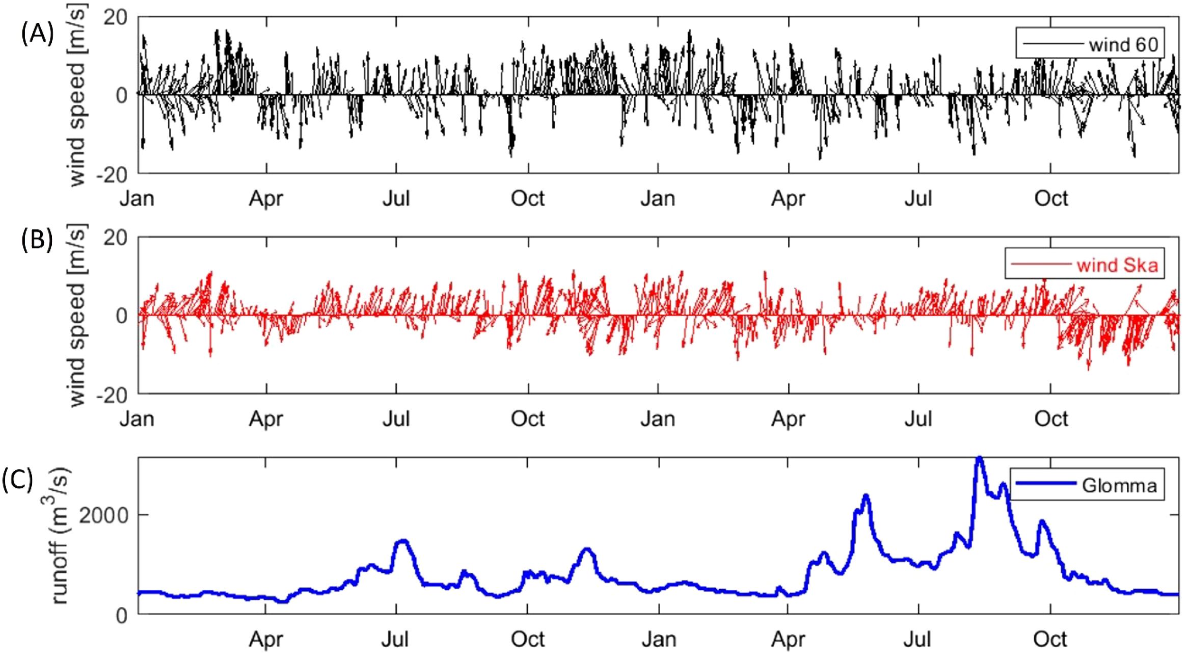
Figure 2. Daily mean wind speed and direction (A) at 60°N and (B) in the Skagerrak over 2022 and 2023. (C) shows the time series of daily mean river discharge from Glomma.

2.2 Analysis

We analyse time series of daily mean model outputs of 2022 and 2023 along four zonal transects extending from 3.9-5.5°E (T1.1) and 2.3-3.9°E (T1.2) at 58.9°N and from 3.9-5.5°E (T2.1) and 2.3-3.°E (T2.2) at 61.28°N (Figure 1B). The location of T1.1 is chosen to capture the NCC without it being strongly entrained by AW. T1.2 is used to capture AW inflow as well as the westwards displacement of the branch of the NCC. The location of T2 is chosen to estimate the cross-shelf exchange based on the data of the northern most flows in the model outputs. T2.1 is selected to capture the NCC outflow towards the north and T2.2 to capture the AW inflow. The total zonal extent of 2.3-5.5°E covers the entire area of the trench but excludes the flows in the North Sea. All parameters are averaged over the zonal extent of the transects which is approximately 100 km. Daily averaged zonal and meridional flow velocities, temperature, salinity, and Eddy Kinetic Energy (EKE) are used in this study. Eddy Kinetic Energy (EKE) is used to identify temporal and spatial distributions of eddies that impact the flow. EKE is defined as “the kinetic energy of the time-varying component of the velocity field” (Martinez-Moreno et al., 2019) and calculated as

$\begin{array}{ll}EKE=\frac{1}{2}(u^{\prime 2}+v^{\prime 2})=\frac{1}{2}{({(u-u_a)}^2+(v-v_a)}^2) & (1)\end{array}$

where $u^{\text{'}2}$ and $v^{\text{'}2}$ are the deviations of daily mean flow velocities ($u$, $v)$ from the annual mean velocities ($u_a,v_a).$ To identify the influence of wind on the flow, we correlate the averaged zonal and meridional flow velocities to the wind time series of 2022 and 2023 at the locations Skagerrak and 60°N. The correlation coefficients (r) of daily averaged wind and flow vectors are calculated based on the Pearson Correlation. We use p = 0.05 as significance threshold, so that r is significant when p < 0.05 and |r| > r (p = 0.05). For the correlation, the averaged velocities over depths from 0 to 400 m are used.

Meridional volumetric transports $(Q_{net})$ ($m^3$/s or in Sv) for 2022 and 2023 are calculated by integrating the averaged velocities in northward $(v_n)$ and southward $(v_s)$ direction along all four transects over depth as

$\begin{array}{ll}{Q}_{n = }\frac{1}{T_a} {\displaystyle {\int }_A{\int }_{T_a}}{v}_n\text{d}A\text{d}t ;\hspace{1em}{Q}_{s = }\frac{1}{T_a} {\displaystyle {\int }_A{\int }_{T_a}}{v}_s\text{d}A\text{d}t & (2)\end{array}$

$\begin{array}{ll} Q_{net = }{Q}_n-Q_s & (3)\end{array}$

with A the cross-sectional area for the transects (T1.1, T1.2, T2.1 and T2.2) and $T_a$ a period of one year (2022 and 2023). Zonal flows are not considered as the dominant exchange flows are in northward and southward direction.

3 Results

3.1 Flow velocities and directions over 2022-2023

We visualize current velocities and directions at 6 locations within the NT for the time span of two years by plotting current roses, see Figure 3. The locations are chosen to cover large parts of the trench and include the outflow area of the NCC as well as the NTI area. The current roses are plotted from the surface data and from data at 150 m depth to show the variation of flows over depth. According to Albretsen et al. (2012), the upper 100 m capture the NCC. The 150 m depth output is well below the 100 m transition and thereby representative for the deeper flow dynamics. The individual time series of flow velocities of all locations are provided in the supplementary material (Supplementary Figures 1, 2). At the surface (Figure 3A), the north-westward flow of the NCC is captured in Station 1. The primarily northward flow of the NCC, following the Norwegian coastline contour in the east, is shown at Stations 3 and 6. These three stations show largest current velocities, exceeding 0.9 m/s. In the West, opposite of the stations which capture the NCC, Stations 2 and 4 show the southward inflow of AW into the trench. In general, the western stations show much lower current speeds than the eastern stations, indicating that the southward inflow of AW is less energetic than the northward outflow of the NCC. At Station 2, the most frequent flow regime is a flow in southeastern to southwestern direction. However, Station 2 also captures strong north-eastward flows with speeds up to 0.45 m/s. Such flows are not present at a depth of 150 m at Station 2; thus, we deduce that they are restricted to the surface only and most probably originate from a westward deviation of a branch of the NCC (Figure 3B). This is further called the westward displacement of the NCC. We do not capture a northward component of the flow at Station 4, but we do at Station 5. At Station 4, the flows are south-eastwards and indicate AW propagation. At Station 5, a strong north-westward flow component is captured, which might result from the western branch of the NCC merging with the more eastern coast parallel branch of the NCC again. At the surface, Stations 3, 4 and 6 show the lowest variability, indicating separate flow pathways of southward directed AW in the west and northward directed coastal waters in the east. Station 1 is slightly more variable compared to Stations 3 and 6, as the extension of the NCC towards the west can vary. At Station 5, the flows are northward across the shelf, but more variable than in the two neighbouring stations. We expect that the variability at Station 5 is due to the alternating occurrence of AW and NCC.

Figure 3

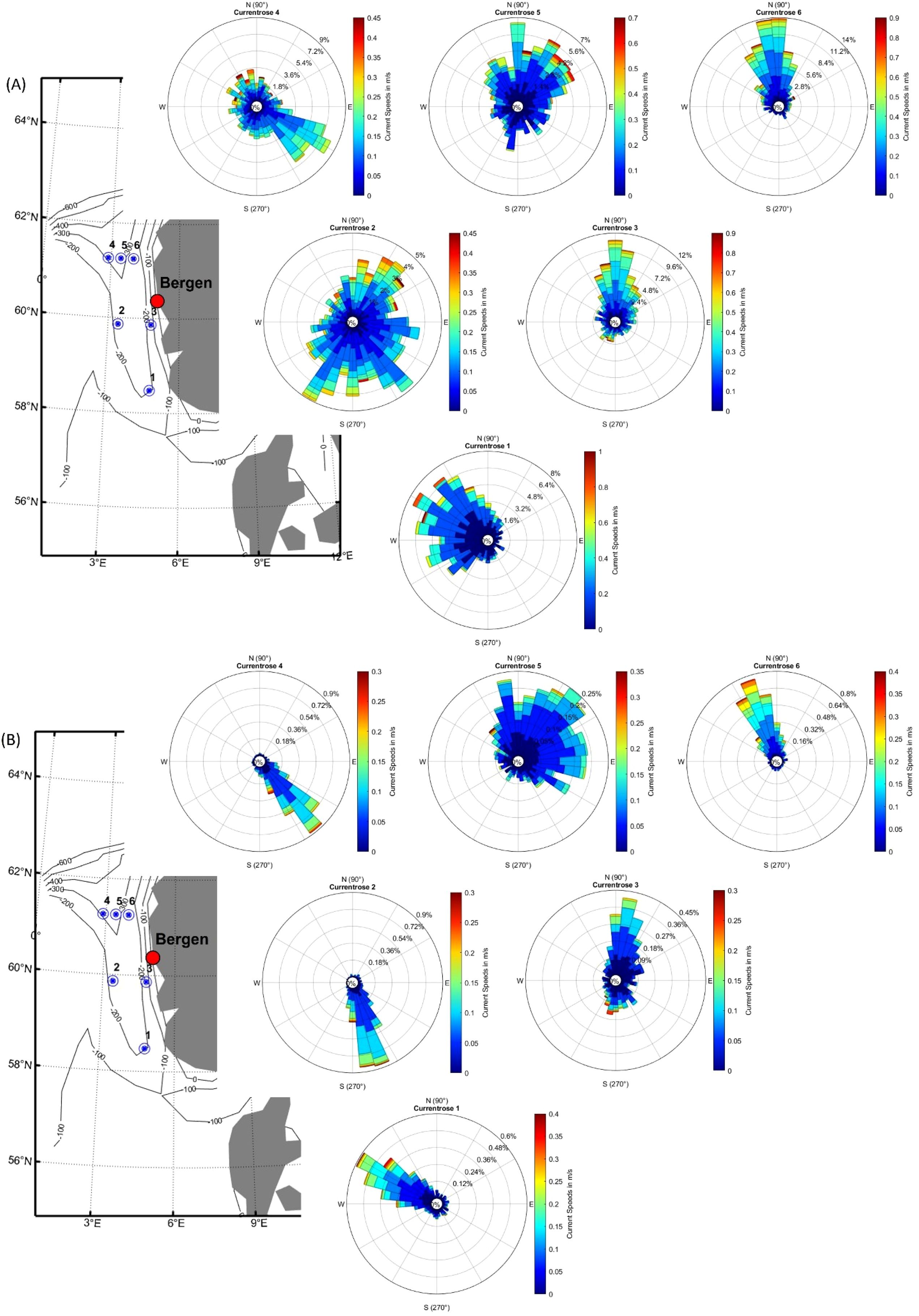
Figure 3. Daily mean current velocities and directions (A) at the surface and (B) at 150 m depth at 6 locations of CMEMS outputs from 01-01–2022 to 31-12 2023. The coordinates are the following: (°N/°E) 1) 58.47/4.81, 2) 59.87/3.42, 3) 59.88/4.81, 4) 61.25/2.86, 5) 61.25/3.42 and 6) 61.25/3.92. For each station, the flow velocity time series has been aggregated into a current rose, indicating the magnitude, direction, and occurrence of flow magnitude and direction in percentage over 2 years. The direction indicates where the flow is going, in contrast to wind roses, which indicate the direction of origin of the wind. We assign North to 90° to point 0° in x-direction.

The current roses at the surface and at 150 m depth show similarities, but also differences. All stations, except Station 5, show low variability at 150 m depth. The variability in the currents is lower at 150 m compared to the surface flows, as the currents are less influenced by winds, topographically steered and restricted by the shape of the canyon itself. The southward inflow of AW is captured in the West (Stations 2 and 4) and the northward outflow of North Sea water in the East (Stations 3 and 6). At Station 1, the flow follows the topography of the trench pointing westwards. At Station 2, the direction of the flow at a depth of 150 m is steered by the topography of the trench, thus only showing the southwards directed AW inflow. At Station 5, the strong variability in eastward direction indicates inflow of AW which is in agreement with the theory of topographic steering at that location. Although the surface and the flows at 150 m depth show similarities in flow direction at Station 5 the mechanisms that steer the flow are very different. At 150 m depth, the NCC does not influence the flow, such that the variability is only related to the redirection of AW and North Sea waters at higher depth. At Station 3, the flow at 150 m depth is mostly northwards, but with some exceptions of strong southward currents. These southwards flows are likely to result from AW inflows which deviate south-eastwards and flow southwards along Station 3. In general, the current roses show that the flow regimes in the NT can be locally very variable and that the forcing of the currents varies over depth.

3.2 Two-year variations along four transects in the NT

Time series of flow velocities and direction, temperature, salinity and EKE (Equation 1) are analysed at the transects T1.1, T1.2, T2.1 and T2.2 (Figures 4, 5) together with wind data from two locations (Figures 2A, B) and river discharge information of Glomma (Figure 2C). As the wind speed and direction are not uniform over our study area, we consider the wind conditions at two locations: Skagerrak and 60°N. We chose 60°N as this represents the upper boundary of our study area and Skagerrak to represent the wind forcing at the location of generation of the NCC. We use three wind events, highlighted with rectangles in Figures 4 and 5, to stress the effect of winds on the flows over two consecutive years. These three main wind conditions are further discussed in Section 3.4.

Figure 4

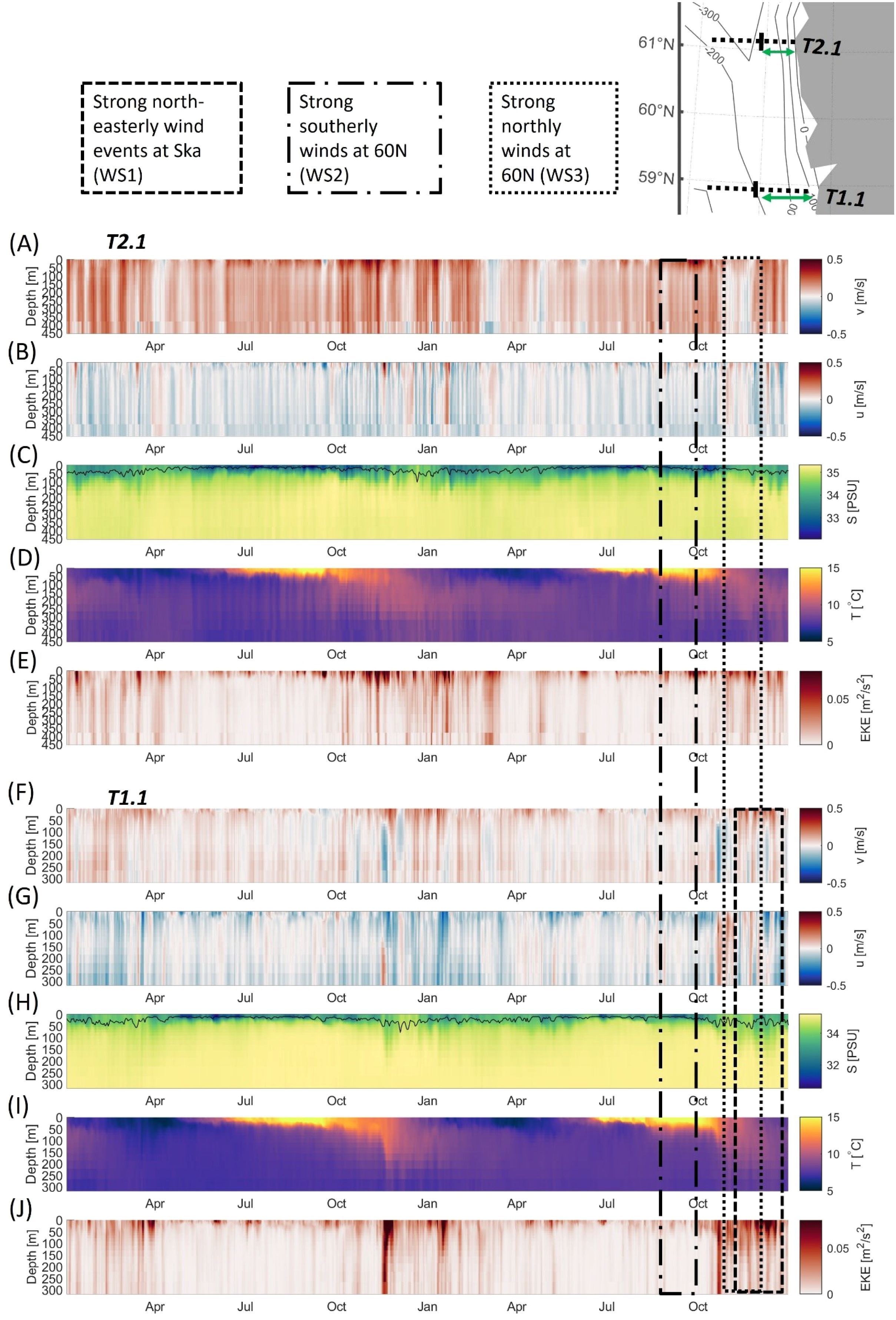
Figure 4. Daily (A) meridional and (B) zonal flow velocities, (C) salinity with MLD (line), (D) temperature and (E) EKE over depths along transect T1.1 (upper) and of (F) meridional and (G) zonal flow velocities, (H) salinity with MLD (line), (I) temperature and (J) EKE over depths along transect T2.1 (lower) for 2022-2023. The small map indicates the location of both transects with green arrows (see Figure 1 for better reference). We present the Wind Scenarios (WS1-3), which are analysed in more detail in Chapter 3.4.

Figure 5

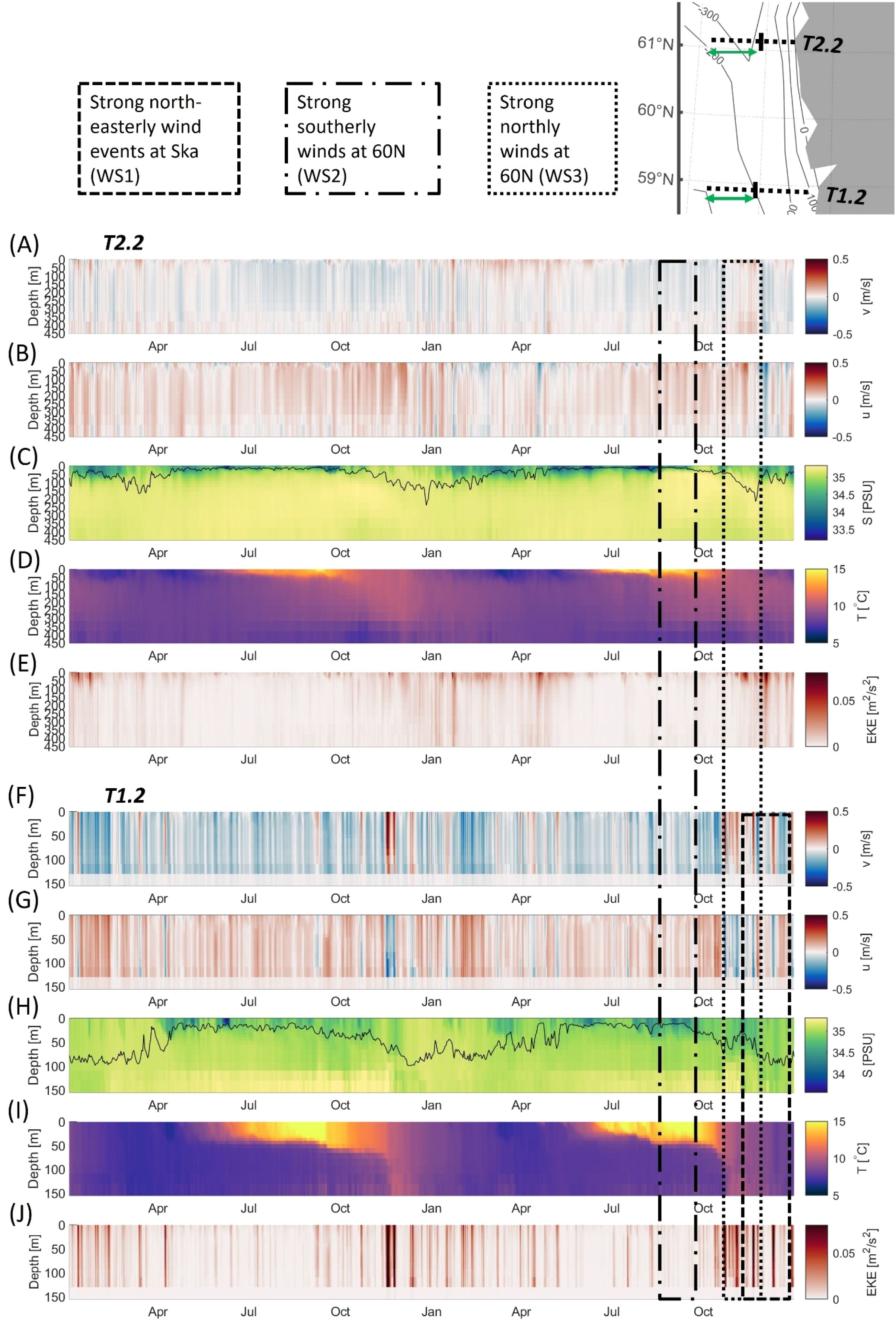
Figure 5. Daily (A) meridional and (B) zonal flow velocities, (C) salinity with MLD (line), (D) temperature and (E) EKE over depths along transect T2.2 (upper) and of (F) meridional and (G) zonal flow velocities, (H) salinity with MLD (line), (I) temperature and (J) EKE over depths along transect T1.2 (lower) for 2022-2023. The small map indicates the location of both transects with green arrows (see Figure 1 for better reference). We present the Wind Scenarios (WS1-3), which are analysed in more detail in Chapter 3.4.

3.2.1 Eastern part of the NT – NCC outflow

The eastern part of the NT shows the north-westward propagation of the NCC and the deeper north-westward outflow of North Sea water in the lower water column (Figures 4A, B, F, G). At both transects, north-westward flow in the upper water column is related to the NCC which flows along the coast of Norway. The NCC, which is visualised by the low surface salinities, is confined to the upper 50 to 100 m of the water column (see MLD in C, H). MLDs in winter extend to a maximum of 50 m and reduce in summer to less than 20 m in both transects. Below the NCC, North Sea water and AW of higher salinity (35 PSU) are flowing north-westwards. However, and especially in winter, south-eastward flow events are happening. At T1.1, south-eastward flows are constrained to the lower water column (> 50 m) and are only rarely visible at the surface where north-westward currents dominate. At T2.1, north-westward flows dominate and are intensified, compared to the southern transect. At T2.1, south-eastward flow events in winter extend over the entire water column. Both transects show intensified flow velocities in winter (October-April) with magnitudes of up to 0.5 m/s whereas in summer (April-October) flow velocities are much lower (< 0.2 m/s). This seasonality coincides with the seasonality of winds, which strengthen over winter and weaken over summer (see Figure 2A, B). At T1.1, large north-westward velocities in the upper 50 m occur during north-easterly winds in the Skagerrak (WS1). These northward velocities are attributed to an outflow of the NCC and are strongest over winter time. At T2.1 maximum north-westward velocities fall together with southerly winds in October 2022-January 2023 and September-October 2023. The strengthening of the flow can either indicate a strengthening of the NCC due to downwelling, or due to flow and wind direction being aligned and thus intensifying the flow (WS2). Largest AW inflows, which extend over the entire lower water column, happen in winter, for example in December 2022 and December 2023, and align with northerly wind conditions (WS3).

In winter, increased flow velocities fall together with increased EKE in both transects (E, J). In winter, high EKE patches extend over the entire water column, whereas in summer, they are restricted to the very shallow surface layers as the water column is stratified, and mixing is suppressed. Increased EKE in summer coincides with increased flow magnitudes and minimal surface salinities (C, H), which are related to fjord or river discharges, for example of Glomma (see Figure 2C). Strong horizontal gradients in sea surface salinity favour the generation of eddies along the eastern side of the trench, whereas strong vertical gradients suppress vertical mixing and confine the influence of wind and atmosphere-ocean exchange to the upper water column. Both transects show surface waters to warm up to 16 °C in summer and cool down to 6 °C in winter (D, I). Increased temperatures in the lower water column over winter could result from the strong AW inflow which brings warmer water into the trench or from convective mixing. Increased MLD over winter in both transects suggest increased vertical mixing, a weakening of the stratification and thus increased heat transport into the lower water column. As the northern transect shows slightly higher temperature over winter in the deep layers but similar MLD, we relate increased temperature over winter to the influence of AW inflow. In December 2022, a strong AW inflow event is detected at T1.1 by south-eastward flows which align with increased MLDs. For depths larger than 100 m there is no seasonality in salinity detected in any of the transects.

3.2.1.1 Correlation at T1.1

Figure 6 shows the correlations between the wind conditions and current velocities over the entire water column at T1.1. We distinguish the wind conditions at the two wind stations Skagerrak (A, B, E, F) and 60°N (C, D, G, H). Each subplot indicates the correlation between the flow velocities in four directions and the given wind direction. Westerly winds at both locations show a positive correlation with all four flow directions, with the eastward flows showing the largest correlation of 0.5 for the westerly wind condition at 60°N and with all correlations increasing with depth (B, D). Easterly winds in the Skagerrak show a peak of positive correlations (0.3-0.4) with all velocities at 50 m (F), while easterly winds at 60°N show maximum correlations at 50 m depth with northward and eastward flows but minimum correlations with southward and westward flows (H). In the Skagerrak, southerly winds correlate with north-westward flows in the lower water column but show no correlation with surface flows (A). At 60°N, southerly winds correlate with positive with eastward flows in the upper water column, following the Ekman profile, and with westward flows in the lower water column (C). At 60°N, northly winds show a negative correlation with northward flows in the upper 50 m and a weak positive correlation with westward flows at depths of 120–220 m (E, G). For northly winds in the Skagerrak, the correlations are similar for northward and eastward flows, both being positive and largest in the upper 50 m, while southward flows show a positive correlation which strengthens with increasing depth.

Figure 6

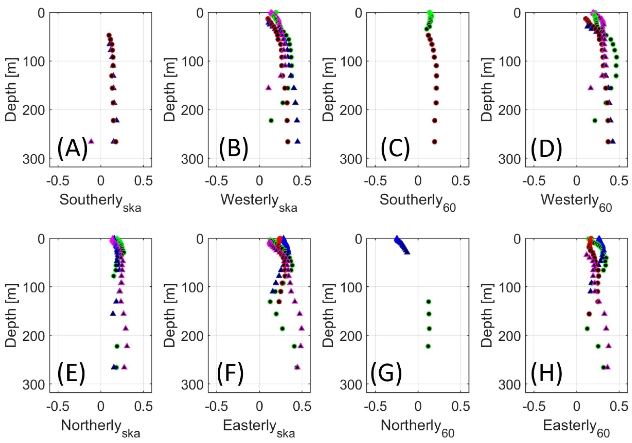
Figure 6. Correlation coefficients over depths are visualized for 8 wind conditions (A-H). The correlation is conducted for eastward (green), northward (blue), westward (red) and southward (magenta) flow velocities over all depth at T1.1. Missing correlation coefficient points indicate that the correlation was not significant.

3.2.1.2 Correlation at T2.1

In Figures 7A-H we show the correlations of winds and flows at T2.1. Westerlies and southerlies at both locations have similar correlations to flows (A-D). Northward and westward flows show low positive correlation at the surface, an increase until 50 m depth and a gradual positive correlation of 0.4-0.5 over the entire water column for westerlies. For southerlies, the profiles are similar, but as depth increases, the correlations stay equal or decrease. For southerly winds, the correlation of the westward velocities is weaker and the peak at 50 m depth for the northward flows is more pronounced. Westerly winds in the Skagerrak and southerly winds at both locations show a negative correlation with southward flows at the surface. For southerly winds in the Skagerrak, the correlation is weak but positive at 150 m. Southerly winds at 60°N show a weak positive correlation with eastward flows in the upper 50 m of the water column. For northerly winds, northward flow shows a negative correlation of -0.2-0.3 over the entire water column at 60°N and over the lower water column (150 m – 400 m) in the Skagerrak (E, G). Southward flows correlate positively with a maximum at 100 m depth. The correlation vanishes with increasing depth in the Skagerrak, but increases at 60°N. At both locations, westward flows show positive correlations with northly winds at the very surface and eastward flows show positive correlations of 0.2-0.3 over the entire water column with northly winds and easterly winds. Easterlies in the Skagerrak correlate positively (0.2-0.3) with southward, northward, and eastward flows (F). The correlation with northward flows is confined to the upper 80 m while southward and eastward flows show correlations until 200–300 m depth. Easterlies at 60°N correlate positively with eastward flows, but show a negative correlation for northward flows at 150–400 m depth (H).

Figure 7

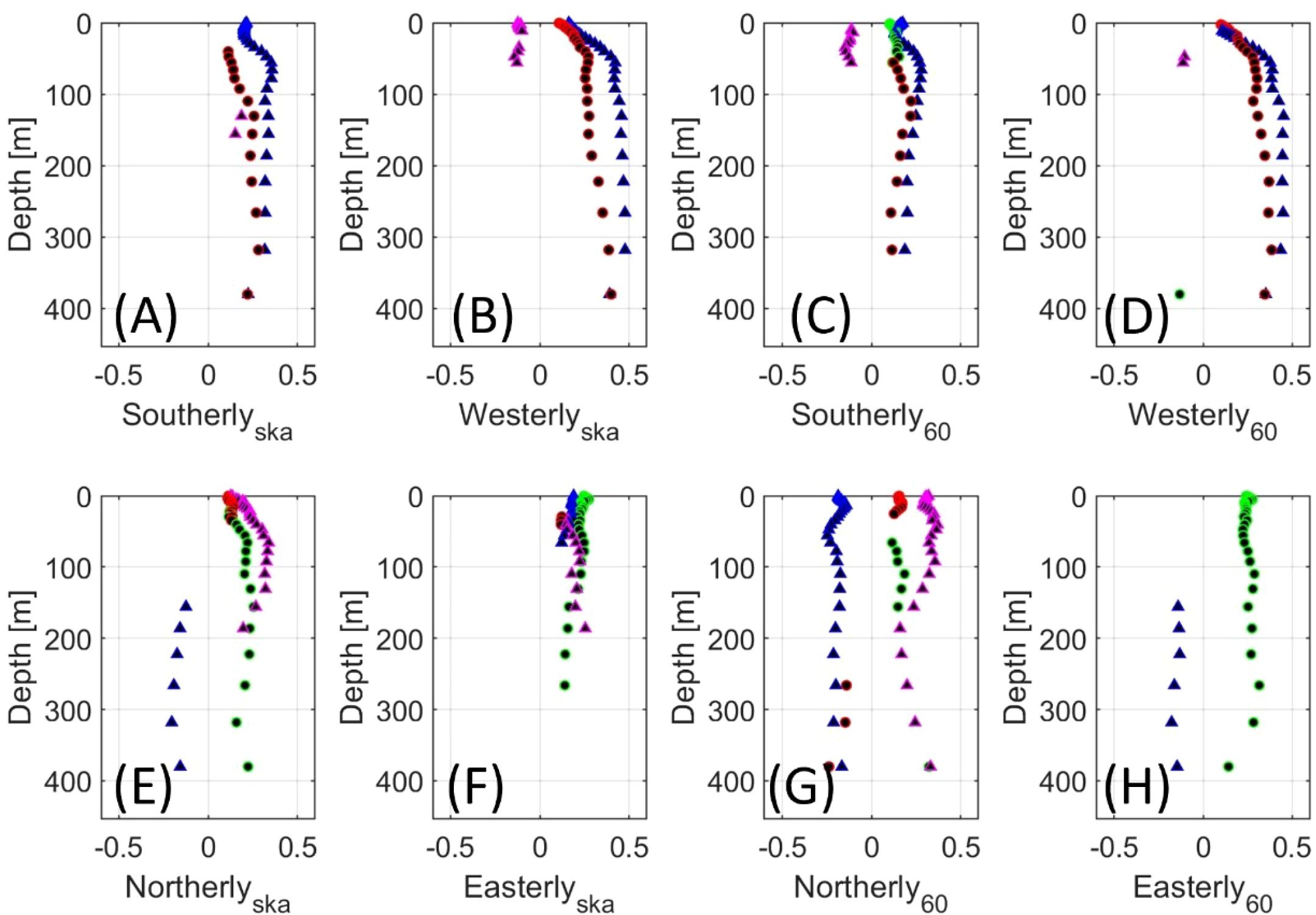
Figure 7. Correlation coefficients over depths are visualized for 8 wind conditions (A-H). The correlation is conducted for eastward (green), northward (blue), westward (red) and southward (magenta) flow velocities over all depth at T2.1. Missing correlation coefficient points indicate that the correlation was not significant.

3.2.2 Western part of the NT - AW inflow

In Figure 5, we show the western transects, which resolve the inflow of AW into the NT. At T1.2, the shallow North Sea shelf is captured, such that when averaging over the transect, the vertical profile of T1.2 only extends to 150 m water depth (F-J). In both transects, the main current direction is south-eastward (A, B, F, G). At the southern transect T1.2 (A, B), the south-eastward flows extend over the entire water column. In the north, at T2.2 (F, G), the water column shows multi-directional flows. Different flow directions at the surface and at higher depth are enabled by the strong salinity stratification (C). In summer (April-October) the currents are southward from the surface down to 350 m depths, and below that north-westwards again. In winter, the surface flows are north-westwards at the surface until 50–100 m depth. Below that depth, the flow either continues in north-westwards direction or changes to a south-eastward direction. At 350 m depth, the direction of flow is north-westward or north-eastward. At T2.2, strong north-westward currents are related to NCC outflows, aligning with low salinity events at the surface (H). In November 2023, while southerly wind conditions predominate (WS2), the westward branch of the NCC is captured at T1.2 by north-westward velocities, which extend over the entire water column. In summer, the water column at T2.2 is stratified by a fresher surface layer and MLDs of 20–50 m indicate a very shallow stratification with low mixing. Below that, the water column is filled with AW and North Sea water. In the two-year time series, there are three events at T2.2 where the surface is not stratified and the MLD deepens to 150–200 m: March-April 2022; winter 2022-2023; and November-December 2023. During these events, EKE increases, but by far not as strongly as observed in the eastern transects (Figure 4E). At T1.2 the MLD is shallow over summer but deepens to 100 m over winter in both years, showing the same seasonality as T2.2. High EKE events happen in winter and align with convective mixing of the water column (I, J). In both transects the seasonality in temperature is remarkably similar to what we observe in Figure 4. However, at T2.2 the lower water column is warmer than elsewhere in the trench (D), which can be related to the proximity of T2.2 to the shelf edge and consequently increased water contribution from the NAC.

3.2.2.1 Correlation at T1.2

Figures 8A-H shows the correlation of winds and current speeds averaged over T1.2. Southerly winds at both locations show a positive correlation of 0.2 with eastward flows over the upper 25–40 m of the water column (A, C). For southerly winds at 60°N, we see a negative correlation with southward flows in the upper meters of the water column. Besides this, any other correlation is absent. Westerly winds at both locations correlate with southward and eastward flows (B, D). The correlation is strongest with 0.6 at the surface and decreases to 0.2-0.3 with increasing depth, showing the shallowness of the surface layer which feels the direct wind impact. Easterly winds show positive correlations with northward and westward flows, both showing strongest correlations of 0.6 at the surface and decreasing correlations with depth (F, H). There is a negative correlation of about -0.3 between easterly winds and southward flows, which decreases with depth. In the Skagerrak, northerly winds show positive correlations with northward and westward flows (0.2), where the latter one only shows a correlation in the upper 40 m of the water column (E, G). Negative correlations with northerly winds are calculated for eastward flows (-0.2) in the upper 40 m and for southward flows in the lower 40–100 m of the water column. At 60°N, northerly winds correlate positively with southward flows throughout the entire water column, with eastward flows at 50–130 m depth and negatively with northward flows in the upper 20 m of the water column.

Figure 8

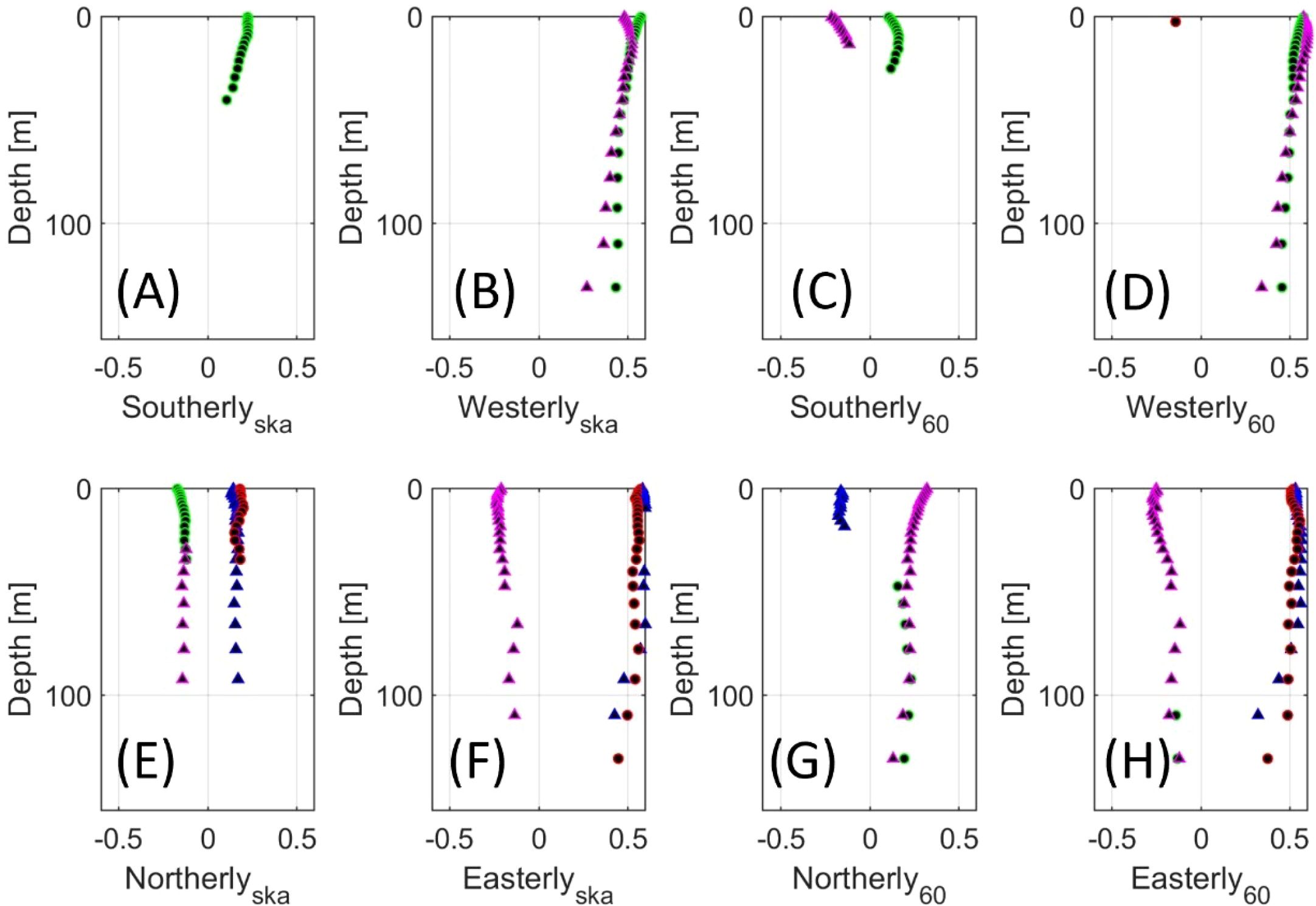
Figure 8. Correlation coefficients over depths are visualized for 8 wind conditions (A-H). The correlation is conducted for eastward (green), northward (blue), westward (red) and southward (magenta) flow velocities over all depth at T1.2. Missing correlation coefficient points indicate that the correlation was not significant.

3.2.2.2 Correlation at T2.2

The correlations of flows and winds at T2.2 is shown in Figures 9A-H. In the Skagerrak and at 60°N, westerly winds show similar correlations with all four flow directions (B, D). Southward flows show largest correlations with westerlies in the surface layer (0.4), a maximum correlation at 50 m depth and a strong decrease of correlation with depth. Compared to that, northward and eastward flows show a minimum in the correlation at 50 m depth. Westward flows in the Skagerrak show a similar correlation profile as the southward flows, only weaker. Easterly winds in the Skagerrak show a positive correlation to southward and eastward flows, with a maximum of 0.4 at 100 m depth (F). Easterly winds at 60°N show a positive correlation with eastward flows in the upper 150 m, but a negative and only very scattered surface correlation to southward flows. Southerly winds in the Skagerrak correlate positively with north-, east- and southward flows, where the latter one shows largest correlation at 30 m depth. Southerlies at 60°N correlate negatively with southward and westward flows at the very surface (A, C). Northward flows show a positive correlation, increasing with depth, while eastward flows a strong positive surface correlation of 0.3, decreasing until vanishing at 100 m depth. Northerly winds at 60°N only show correlations in the upper 50 m of the water column, which are negative for eastward flows, and positive for northward, southward, and westward flows (G). In the Skagerrak, northerlies correlate positively over the entire water column, with all flow directions showing largest correlations at the surface, especially for westward flows with 0.3. All correlations decrease at 50 m but continue between 0.1-0.3 until 200 m for northward and eastward flows, and until 300–400 m for southward and westward flows (E).

Figure 9

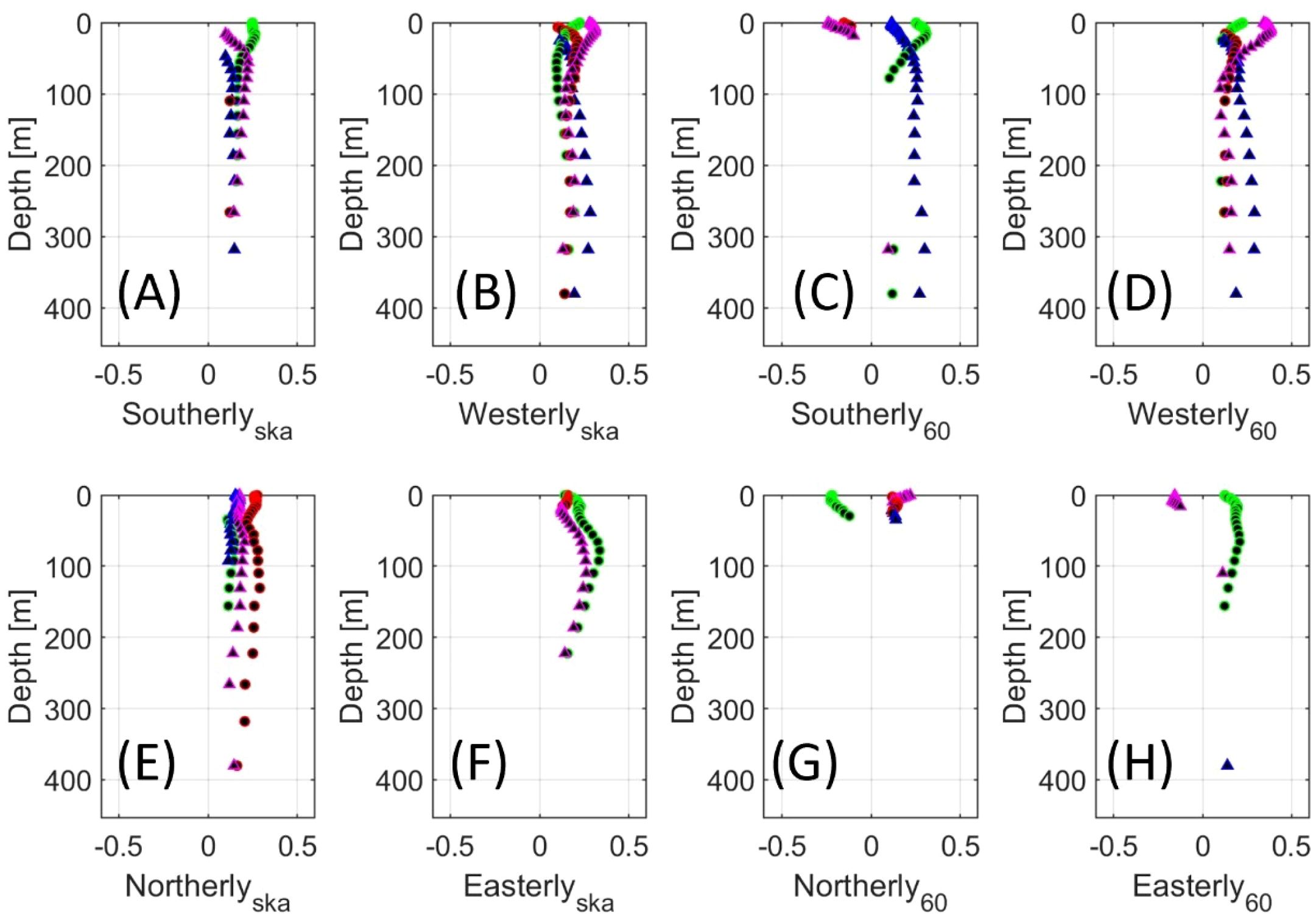
Figure 9. Correlation coefficients over depths are visualized for 8 wind conditions (A-H). The correlation is conducted for eastward (green), northward (blue), westward (red) and southward (magenta) flow velocities over all depth at T2.2. Missing correlation coefficient points indicate that the correlation was not significant.

3.3 Transports in 2022 and 2023

Net volumetric transports are calculated at each transect for 2022 and 2023 over the upper 400 m of the water column (Table 1; Equations 2, 3). In Figure 10 we show the daily transports at each of the transects (A-D) but separated for transport above and below the MLD. Table 1 shows that in- and outflows at T1 (T1.1 and T1.2) compensate, such that the net transports in 2022 and 2023 are low across the southern transect T1. T1.1 shows positive northward transports for both years, while transports at T1.2 are of the same magnitude but southwards. In Figure 10, largest transport magnitudes are calculated in winter and are in northward direction at T1.1 (A), whereas at T1.2 (B), southward directed transports dominate, except in winter where largest magnitudes are northwards. We show that at the eastern side of the NT (T1.1 and T2.1) the surface transports are northwards, but that below the MLD, in-and outflows in southward and northward direction balance. At T1.2, the southward transports above and below the MLD contribute to the net southward transport and are only compensated for by northward transports in winter. At T2 (T2.1 and T2.2) northward transports dominate. At T2.1 the northward transport is much larger and not compensated by the inflow at T2.2 (Table 1). At T2.1 the large contribution of positive meridional transport below the MLD is the main source of the large transport volume (C). Transports above the MLD are small in comparison. Both northern transects show a strong seasonality, with increased winter transports in both directions, especially for transports above the MLD. At T2.1, the seasonality in northward transports below the MLD is largest with a maximum of 10 Sv in winter 2022. The transport profile of T2.2 is very similar to that of T1.1, showing balanced conditions for in- and outflows below the MLD. Taking all transects into account, the net meridional transports over both years are 2–3 Sv.

Table 1

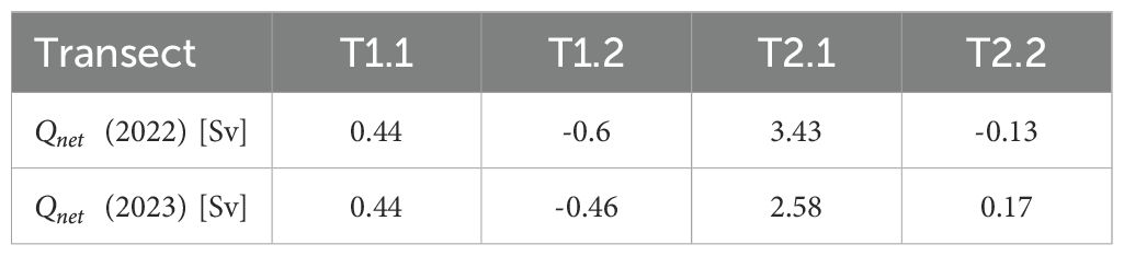
Table 1. Net transports ($Q_{net}$) calculated with equation 3 at all transects over 2022 and 2023.

Figure 10

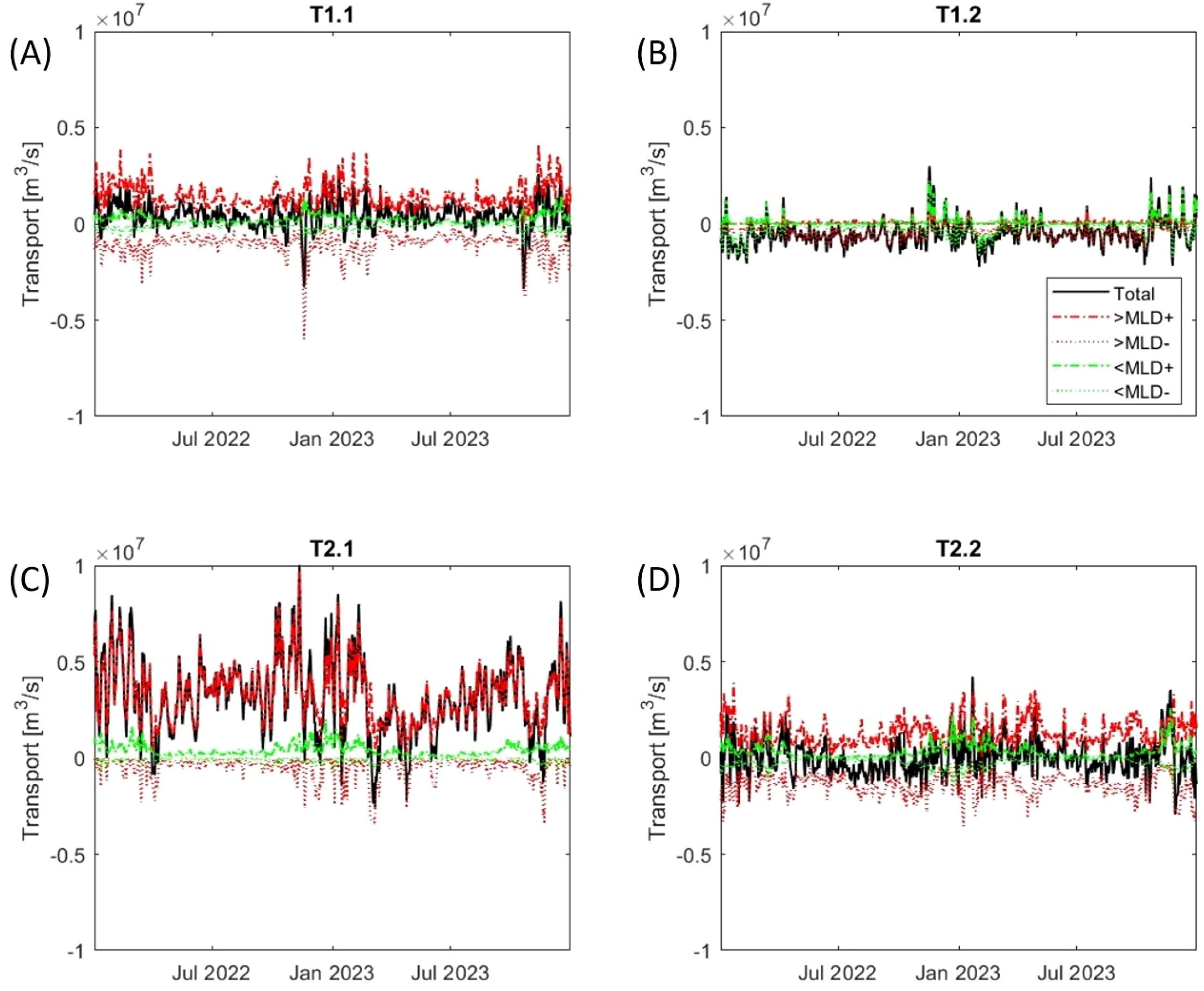
Figure 10. Daily transports for all transects (A-D) over 2022 and 2023. Transport above the MLD (< MLD) is contributed by the NCC, whereas transport below the MLD (> MLD) is related to North Sea and AW transport.

3.4 Flow and wind scenarios in the NT

From the relations identified in Section 3.2, we create scenarios that capture the largest wind-induced variability of the flows in our study area over winter. Wind Scenario WS1 (Figure 11) shows the NCC outflow during north-easterly winds in the Skagerrak. Wind Scenario WS2 (Figure 12) captures strong northward currents during southerly winds and Wind Scenario WS3 (Figure 13) reveals the deep AW inflow during northerly winds in wintertime. These scenarios illustrate the most energetic inflow and outflow conditions of the NT and can therefore be used to explain the short-term variations in cross-shelf exchange flows. The response of the hydrodynamics to these wind conditions is presented for characteristic days (see Figures 4, 5). We acknowledge that there are other wind scenarios and that seasonality in flow patterns is large, but a full discussion of all possible wind scenarios is beyond the scope of this study. Instead, we selected wind conditions during some days in winter 2023, to show the influence of wind under the same year and seasonal circumstances.

Figure 11

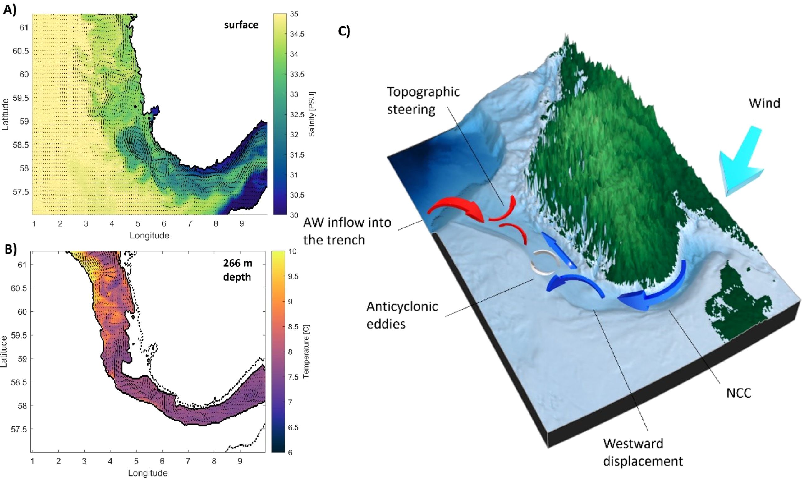
Figure 11. Contour plots of (A) surface salinity and (B) temperature at 266 m depth for WS1 (December 1^st, 2023). Current velocities (arrows) have maximum velocity at the surface of 1 m/s and of 0.5 m/s at depth. (C) We schematize the flows and the prevailing wind direction on a topographic map provided by GEBCO (GEBCO Compilation Group, 2024).

Figure 12

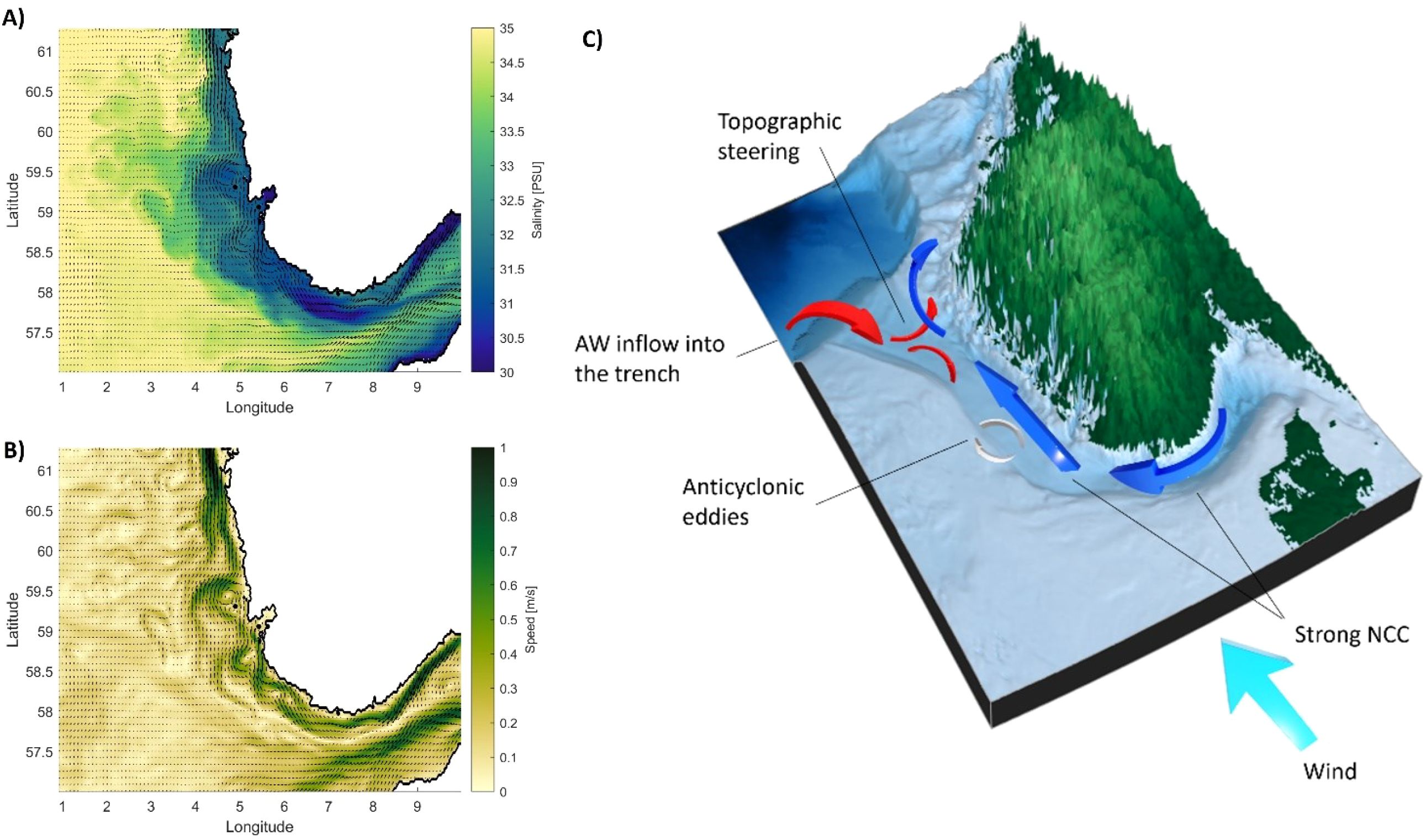
Figure 12. Contour plots of (A) surface salinity and (B) surface current velocities for WS2 (September 27^th, 2023). Current velocities (arrows) have maximum velocity at the surface of 1 m/s. (C) We schematize the flows and the prevailing wind direction on a topographic map provided by GEBCO (GEBCO Compilation Group, 2024).

Figure 13

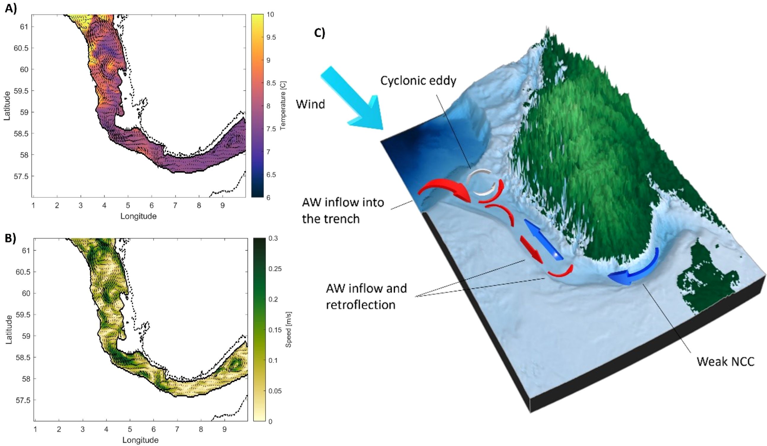
Figure 13. Contour plots of (A) temperature and (B) current velocity at 266 m depth for WS3 (November 25^th, 2023). Current velocities (arrows) have maximum velocity of 0.5 m/s at depth. (C) We schematize the flows and the prevailing wind direction on a topographic map provided by GEBCO (GEBCO Compilation Group, 2024).

For WS1, we selected a representative day in 2023, where north-easterly winds dominate in the Skagerrak and northerly wind conditions at 60°N (Figure 11). These two wind conditions often occur together, especially in winter (see Figures 2A, B). Increased inflow during northerly winds and outflow during north-easterly winds might be one of the main reasons why transports above and below the MLD mostly compensate (Figure 10). During WS1, the NCC enters the trench as a large freshwater plume with current speeds of 1 m/s at the surface from the Skagerrak in the East (A). A clockwise rotating eddy (anticyclone) is generated in the NCC at 58°N. The horizontal salinity gradient between the NCC and AW in zonal direction, is largest in the south of the trench and weakens towards the north. Due to mixing of the NCC with the AW and the lack of sufficient freshwater input, eddies are not generated frequently at higher latitudes. On that day, the NCC is displaced towards the west, which is very typical during easterly and southerly winds. At 266 m depth current velocities are weaker with a maximum velocity magnitude of 0.5 m/s (B). Large velocity magnitudes are induced by the inflow of AW in the northwest of the NT and around the topographic barrier at 58.5°N. This is a frequently occurring velocity distribution. The direction of flow is northward in large parts of the trench, except for the southward directed AW inflow in the northwest. NTIs that do not propagate far south in the NT but are redirected eastwards, explain averaged annual transport conditions. The southward flowing water is deflected to the east before reaching 58°N and merges with the northward flow of the North Sea water on the eastern side of the trench, contributing to a net northward transport across the shelf (see Figure 10). As the topographic barrier confines the northward flow, it intensifies the North Sea flows and blocks the AW from flowing southwards.

WS2 shows the response of the surface currents to southerly winds (Figure 12). Southerly winds are dominant in summer (April-October 2022 and 2023) but can also happen in winter. In Figure 12, we see that the NCC is narrow and confined against the coast in the north of the NT. Current velocities reach maximum velocities of 1 m/s. In the rest of the NT the NCC is meandering and the largest velocities of just less than 1 m/s occur at the edges of mesoscale eddies. The strong and confined NCC at the surface indicates downwelling conditions which are induced by onshore/eastward Ekman transport (see Figure 7C). We do not show the flows at higher depth here as they fall into the category of the conditions described in Figure 11, with dominant northward outflow of North Sea waters in the east of the trench and southward inflowing AW in the northwest of the trench.

In Figure 13, we show large NTIs which occur rarely, and only in winter during northly wind (WS3). These inflow events can be identified by an increase of temperature due to inflow of new AW from the NAC (A). Under strong NTI conditions the AW propagates until 58°N and is either redirected eastward by the topographic barrier or overflows it in southward direction. The magnitude of the southward directed current increases as it flows around the sill, often triggering cyclonic vortices nearby (B). The northward flow around the sill is suppressed. At the northern edge of the NT, an anticlockwise (cyclonic) eddy can be seen for some days of the simulation outputs, especially during AW inflows. Flow velocities in the vicinity of the eddy and of the topographic barrier reach magnitudes of 0.3 m/s close to the bed. The diameter of the eddy is restricted by the width of the trench, which at 61°N approximates 100 km. The location of the eddy and its diameter do not change over the two years of simulation output, yet its intensity changes in proportion to the strength of the inflow and outflow at higher depth. In the Skagerrak, another cyclonic eddy is captured, this one smaller with a diameter of around 50 km.

4 Discussion and conclusion

The results of our two-year analysis provide new insights into the flow dynamics of the NT. Our analysis shows that the NT is a very dynamic system, with wind and seasonality driving flows at the surface and at larger depths. In the East, the NCC flows northwards in the upper 50–100 m of the water column (Figure 3, Stations 3 and 6). The westward displacement of the NCC which is discussed in Ikeda et al. (1989), is captured in the current roses, as well as along the western transect T1.2 in Figure 5. Westwards propagation of the NCC coincides with easterly wind conditions (Figures 9, 11), which are also identified to be the main wind direction to cause strong NCC outflows in the Skagerrak (Figure 4). In the West, the NTI of AW is captured at the surface and at higher depth (Figure 3, Stations 2 and 4). The retroflection of AW, first described by Furnes et al. (1986), is identified in the model outputs in Figures 4 and 11. At T1.1 flows in south-eastward direction indicate the eastward retroflection of southward flowing AW. The current rose of Station 5 shows the topographically steered flow in the North, resulting in an eastward redirection of the flow, as described in Johannessen et al. (1989) (Figure 3).

From this two-years analysis we see that the intra-annual variation is low. This finding is supported by studies that calculated similar transports in very different years. In agreement with others, e.g. Winther and Johannessen (2006); Christensen et al. (2018) and Huthnance et al. (2009), we calculated the net transport through the NT to be 2–3 Sv. We identify that seasonal variations are much larger than intra-annual variations (Figure 10) which agrees with Winther and Johannessen (2006). Largest transports happen over winter, in both, northward and southward direction, below and above the MLD. In general, this indicates an intensification of flows over the entire North Sea domain during winter time.

Several studies related the transports in the NT to the large-scale meteorological forcing of the NAO. The NAO is known to impact the flows of the North Sea and North Atlantic in a seasonal cycle, especially strengthening them over winter (Winther and Johannessen, 2006; Christensen et al., 2018; Albretsen et al., 2012). Aagaard (1970) observed that the spatial pressure distribution over the Norwegian Seas varies over seasons and the flows are to a substantial extent wind-driven. For weekly to monthly time scales, Winther and Johannessen (2006) show significant correlation between the transport of the NCC and the NAO. Albretsen et al. (2012) show correlations of AW inflow into the North Sea and winter NAO (NAO index from December to March). Strong westerly wind conditions, which are predominant during positive winter NAO, intensify the NAC which carries warmer water into the North Sea. Our results also show warmer deep-water inflows over winter during northerly and north-westerly winds which we classify as intensified AW inflows, as presented in WS3 (Figure 13). We acknowledge that convective mixing could also be responsible for increased water temperatures at higher depth in winter. In Figures 4 and 5, we show increased MLD over winter, indicating intensified mixing. However, the contribution of one or the other process is not quantified here. A connection of the NTIs to the NAO is reasonable, as the relation of NAO is strongest over longer (yearly, decadal) time scales and often used as a predictor of North Atlantic flows (Winther and Johannessen, 2006). What we explore here are NTIs that reach southward but are not as strong as to reach the Skagerrak. However, we expect these inflows to contribute to the salt budget of the North Sea and to its bio-chemical system (Van Der Molen and Paetsch, 2022).

For the first time, we discuss a deep cyclonic eddy, which is captured by the model at the mouth of the NT during WS3. This eddy is strongest during large AW inflows, as shown by the coinciding increases of flow magnitude and temperature (Figure 13). We doubt that its generation is solely caused by topographic steering (Johannessen et al., 1989) but that it might be created by the canyon-like shape of the NT. Mork (1981) already mentioned that the role of the bottom topography needs to be explained in more detail to understand the presence of trapped vortices at high depth. His suggestion is based on the study of Eide (1979) who discusses the topographically induced eddy generation along the Norwegian coastline. However, the eddy visible in the model has not been discussed before and neither has its generation. In the North, the topography of the NT is similar to a canyon, as the slopes towards the shelf in the West and towards Norway in the East function as barriers to the flow. Inflows into the NT are redirected either by the topographic barrier (Furnes et al., 1986) or by topographic steering, creating a cyclonic circulation at the mouth of the canyon. We suggest that these two effects might be further influenced by dynamics inherent to canyon flows. The generation of large eddies at the mouth of or within canyons is described in Allen et al. (2001). Christensen et al. (2018) investigated the cyclonic eddy, which is present in the Skagerrak under certain conditions, however without attributing its generation to canyon flows. Davies and Heaps (1980) could simulate the cyclonic eddy in the North in a very simplified model. They related its generation solely to the wind-driven currents in the North Sea.

In our study we use EKE to identify surface eddies. Increased EKE coincides with outflows of the NCC (Figures 4, 5). Hence, we conclude that the generation of eddies, caused by the density difference of the NCC and AW is resolved in the model (Tonani et al. (2019); Ikeda et al. (1989); Akpınar et al. (2022)). Largest density differences of AW in the West and fresher water in the East happen in summer. Increased river discharges, for example from Glomma, contribute to a freshening of the surface waters in the eastern part of the NT and can cause baroclinic instabilities, which result in eddy generation. Based on the findings of Johannessen (1986), fjord outflows are seasonal, such that the effect might be very similar to the one of river discharge presented in this study. Johannessen (1986) suggests that during summer, fjord discharges with salinities of less than 32 PSU contribute to a freshening of the NCC. The very fresh surface waters, which are mostly visible at 58°N, might discharge from the Stavanger fjord, and might be one of the main reasons why the most stable eddies are generated at that latitude. We suggest that further research should include the contribution of eddies to the total net transport of the NT, and a more detailed investigation of the influence of eddies on the deeper water column.

Finally, our research findings in Section 3.2 show that the flows in the NT are wind-driven. These findings agree with previous studies. Davies and Heaps (1980); Mork (1981); Huthnance et al. (2009); Hordoir et al. (2013) and Christensen et al. (2018) discussed wind as the dominant forcing to explain the variability of flows in the NT. However, the question of how wind influences the flow under consideration of other variables, such as the topography of the NT or seasonal changes, remained unanswered. We state that the effect of wind is significant, also under consideration of the deepening of the trench towards the North (Mork, 1981), the seasonality of the flow (Johannessen et al., 1989) and a more complex model (Davies and Heaps, 1980). As shown by Akpınar et al. (2022), the wind is not uniform over the NT area, often showing a dipole pattern. To capture the effect of wind forcing, we suggest that at least two stations are needed, for example Skagerrak and 60°N. Some of the correlations presented in Figures 6, 7 and 8, 9 show different patterns depending on the wind location that was chosen. Figure 6 (T1.1) shows the wind-driven onset of the NCC via a positive correlation of north-eastward flows during easterly winds in the Skagerrak and at 60°N. The correlation is of r=0.3 at 20–40 m depths, which corresponds to the depths of the NCC. As the correlation decreases with increasing depth, the results show that it is really the surface layer which is impacted by NCC outbreaks in the Skagerrak. In agreement with Winther and Johannessen (2006) and Hordoir et al. (2013), the results show that easterly winds are the main wind direction enabling large freshwater plumes to leave the Skagerrak and form the NCC. On the other hand, westerly winds show high correlations of r=0.4-0.5 with all flow directions below 50 m depth, but low correlations at the surface. Both, AW and North Sea water are influenced by westerly wind conditions. We believe that a proportion of the deeper water in the NT is AW coming from the North Sea shelf, as the correlation for westerlies and south-easterly flows is large in T1.2. The decrease of impact of easterly winds towards the North, agrees with Christensen et al. (2018) and Davies and Heaps (1980). We observe large correlations of north-eastward flows with westerly and southerly winds at the surface. As shown in WS2, the NCC is confined against the coast during south-westerly wind conditions which is in agreement with Huthnance et al. (2009). Furthermore, they identify that during westerly winds, eastward flows cause downwelling conditions along the Norwegian coast. Hordoir et al. (2013) identified that during coast parallel winds (southerlies), increased flow velocities are related to the fact that Kelvin waves propagate in the same direction as the wind is forcing the flow. Our results agree with that, showing intensified northward flow during southerly winds. In Figure 9 (T2.2) the AW inflows at the surface are visualized by a positive correlation of southward flows during westerly winds which is in agreement with Winther and Johannessen (2006), who suggest that the AW inflow is driven by westerly winds.

Overall, we found that the cross-shelf exchange through the NT is driven by the prevailing wind system over the North Sea. We show that that the sensitivity of both the AW inflow and the NCC outflow to wind forcing determines the chaotic nature of the currents in the NT. Since inflow and outflow impact each other, wind forcing on either the inflowing or outflowing currents causes a reaction throughout the NT. The seasonality in wind and river discharge, make the currents in the NT respond to the seasonal cycle over both years. The average annual transports for 2022 and 2023 suggest net northward outflows of 2–3 Sv into the Atlantic Ocean. Over annual time scales, these transports are constant, but variations over days, can be more than three times as large. On daily timescales, surface eddies play a significant role in increasing surface velocities, which consequently lead to increased transport through the NT.

Data availability statement

The original contributions presented in the study are included in the article/Supplementary Material. Further inquiries can be directed to the corresponding author.

Author contributions

AE: Conceptualization, Investigation, Writing – review & editing, Methodology, Writing – original draft, Visualization, Formal Analysis. JP: Supervision, Writing – review & editing. BP: Supervision, Writing – review & editing.

Funding

The author(s) declare financial support was received for the research and/or publication of this article. This publication is part of the program “The role of the North Sea in the Atlantic Ocean biogeochemical system: North Sea-Atlantic Exchange (NoSE)” with file number OCENW.XL21.XL21.075 which is financed by the Dutch Research Council (NWO).

Acknowledgments

We would like to thank all collaborators within the NoSE project who contributed to this study. We would also like to thank Matthew Humphreys for sharing the script to plot the 3D bathymetry data. Finally, we would like to thank the reviewers for their valuable comments and final contributions.

Conflict of interest

The authors declare that the research was conducted in the absence of any commercial or financial relationships that could be construed as a potential conflict of interest.

Generative AI statement

The author(s) declare that no Generative AI was used in the creation of this manuscript.

Any alternative text (alt text) provided alongside figures in this article has been generated by Frontiers with the support of artificial intelligence and reasonable efforts have been made to ensure accuracy, including review by the authors wherever possible. If you identify any issues, please contact us.

Publisher’s note

All claims expressed in this article are solely those of the authors and do not necessarily represent those of their affiliated organizations, or those of the publisher, the editors and the reviewers. Any product that may be evaluated in this article, or claim that may be made by its manufacturer, is not guaranteed or endorsed by the publisher.

Supplementary material

The Supplementary Material for this article can be found online at: https://www.frontiersin.org/articles/10.3389/fmars.2025.1600994/full#supplementary-material

Supplementary Figure 1 | Supplementary plot of flow velocities timeseries for all six current rose stations presented in Figure 3A.

Supplementary Figure 2 | Supplementary plot of flow velocities time series for all six current rose stations presented in Figure 3B.

References

Aagaard K. (1970). Wind-driven transports in the Greenland and Norwegian seas. Deep Sea Research and Oceanographic Abstracts. 17, 281–291. doi: 10.1016/0011-7471(70)90021-5

Crossref Full Text | Google Scholar

Akpınar A., Palmer M. R., Inall M., Berx B., and Polton J. (2022). Locally modified winds regulate circulation in a semi-enclosed shelf sea. J. Geophysical Research: Oceans 127, 1–12. doi: 10.1029/2021JC018248

Crossref Full Text | Google Scholar

Albretsen J., Aure J., Sætre R., and Danielssen D. S. (2012). Climatic variability in the Skagerrak and coastal waters of Norway. ICES J. Mar. Sci. 69, 758–763. doi: 10.1093/icesjms/fsr187

Crossref Full Text | Google Scholar

Allen S. E., Vindeirinho C., Thomson R. E., Foreman M. G. G., and Mackas D. L. (2001). Physical and biological processes over a submarine canyon during an upwelling event. Can. J. Fisheries Aquat. Sci. 58, 671–684. doi: 10.1139/f01-008

Crossref Full Text | Google Scholar

Aznar R., Castrillo-Acuña L., Reffray G., Escudier R., Sotillo M. G., and Cailleau S. (2025). Atlantic - European North West Shelf - Ocean Physics Analysis and Forecast Product NWSHELF_ANALYSISFORECAST_PHY_004_013. Issue 1.3. Mercator Ocean International, Toulouse, France.

Google Scholar

Christensen K. H., Sperrevik A. K., and Brostroem G. (2018). On the variability in the onset of the norwegian coastal current. J. Phys. Oceanography 48, 723–738. doi: 10.1175/JPO-D-17-0117.1

Crossref Full Text | Google Scholar

CMEMS_1. (2025). NWSHELF_ANALYSISFORECAST_PHY_004_013 [Dataset]. E.U. Copernicus Marine Service Information (CMEMS). Marine Data Store (MDS). doi: 10.48670/moi-00054 (Accessed April 22, 2024).

Crossref Full Text | Google Scholar

CMEMS_2. (2024). WIND_GLO_PHY_L4_MY_012_006 [Dataset]. E.U. Copernicus Marine Service Information (CMEMS). Marine Data Store (MDS). doi: 10.48670/moi-00185 (Accessed April 28, 2025).

Crossref Full Text | Google Scholar

Davies A. M. and Heaps N. S. (1980). Influence of the Norwegian Trench on the wind-driven circulation of the North Sea. Tellus 32, 164–175. doi: 10.3402/tellusa.v32i2.10491

Crossref Full Text | Google Scholar

Eide L. I. (1979). Evidence of a topographically trapped vortex on the Norwegian continental shelf. Deep-Sea Res. 26, 601–621. doi: 10.1016/0198-0149(79)90036-0

Crossref Full Text | Google Scholar

Furnes G. K., Hackett B., and Sætre R. (1986). Retroflection of atlantic water in the norwegian trench. Deep-Sea Res. 33, 247–265. doi: 10.1016/0198-0149(86)90121-4

Crossref Full Text | Google Scholar

GEBCO Bathymetric Compilation Group (2024). The GEBCO_2024 Grid - a continuous terrain model of the global oceans and land. NERC EDS British Oceanographic Data Centre NOC doi: 10.5285/1c44ce99-0a0d-5f4f-e063-7086abc0ea0f

Crossref Full Text | Google Scholar

Giesen R., Stoffelen A., and Verhoe A. (2024). For global ocean hourly sea surface wind and stress from scatterometer and model products WIND_GLO_PHY_L4_NRT_012_004 WIND_GLO_PHY_L4_MY_012_006. Toulouse, France: Mercator Ocean International

Google Scholar

Global Runoff Data Centre. “BfG-department M4 “Geodata center, wasserBLIck, GRDC,” in Imprint – global runoff data centre (Koblenz, Germany: World Meteorological Organization (WMO) at the Federal Institute of Hydrology).

Google Scholar

Hordoir R., Dietrich C., Basu C., Dietze H., and Meier H. E. M. (2013). Freshwater outflow of the Baltic Sea and transport in the Norwegian current: A statistical correlation analysis based on a numerical experiment. Continental Shelf Res. 64, 1–9. doi: 10.1016/j.csr.2013.05.006

Crossref Full Text | Google Scholar

Hovland M. and Indreeide A. (1980). Detailed sea bed mapping for a pipeline across the Norwegian Trench. Int. Hydrographic Rev. LVII, 101.

Google Scholar

Huthnance J. M., Holt J. T., and Wakelin S. L. (2009). Deep ocean exchange with west-European shelf seas. Ocean Sci. 5, 621–634. doi: 10.5194/os-5-621-2009

Crossref Full Text | Google Scholar

Huthnance J., Hopkins J., Berx B., Dale A., Holt J., Hosegood P., et al. (2022). Ocean shelf exchange, NW European shelf seas: Measurements, estimates and comparisons. Prog. Oceanography 202, 102760. doi: 10.1016/j.pocean.2022.102760

Crossref Full Text | Google Scholar

Ikeda M., Johannessen J. A., Lygre K., and Sandven S. (1989). A process study of mesoscale meanders and eddies in the norwegian coastal current. J. Phys. Oceanography 19, 20–35. doi: 10.1175/1520-0485(1989)019<0020:APSOMM>2.0.CO;2

Crossref Full Text | Google Scholar

Johannessen O. M. (1986). “Brief overview of the physical oceanography,” in The nordic seas, chapter 4 (Springer-Verlag New York Inc). Ed. Hurdle B. G.

Google Scholar

Johannessen J. A., Svendsen E., Sandven S., Johannessen O. M., and Lygre K. (1989). Three-dimensional structure of mesoscale eddies in the norwegian coastal current. J. Phys. Oceanography 19, 3–19. doi: 10.1175/1520-0485(1989)019<0003:TDSOME>2.0.CO;2

Crossref Full Text | Google Scholar

Martínez-Moreno J., Hogg A. M., Kiss A. E., Constantinou N. C., and Morrison A. K. (2019). Kinetic energy of eddy-like features from sea surface altimetry. J. Adv. Modeling Earth Syst. 11, 3090–3105. doi: 10.1029/2019MS001769

Crossref Full Text | Google Scholar

McClimans T. A., Eidnes G., and Moshagen H. (2009). “Extreme bottom currents along a deep fjord pipeline route,” in Proceedings of the Nineteenth (2009) International Offshore and Polar Engineering Conference, Osaka, Japan.

Google Scholar

McClimans T. A. and Lonseth L. (1985). Oscillations of frontal currents. Continental Shelf Res. 4, 699–707. doi: 10.1016/0278-4343(85)90037-8

Crossref Full Text | Google Scholar

McClimans T. A., Pietrzak J. D., Huess V., Kliem N., Nilsen J. H., and Johannessen B. O. (2000). Laboratory and numerical simulation of the Skagerrak circulation. Continental Shelf Res. 20, 941–974. doi: 10.1016/S0278-4343(00)00007-8

Crossref Full Text | Google Scholar

Mork M. (1981). Circulation phenomena and frontal dynamics of the norwegian coastal current. Philos. Trans. R. Soc. London. Ser. A 302, 635–647. doi: 10.1098/rsta.1981.0188

Crossref Full Text | Google Scholar

Pawlowicz R. (2020). "M_Map: A mapping package for MATLAB", version 1.4m. Available online at: www.eoas.ubc.ca/~rich/map.html (Accessed September, 2024).

Google Scholar

Sætre R., Aure J., and Ljoen R. (1988). Wind effects on the lateral extension of the Norwegian Coastal Water. Continental Shelf Res. 8, 239–253. doi: 10.1016/0278-4343(88)90031-3

Crossref Full Text | Google Scholar

Skagseth Ø., Drinkwater K. F., and Terrile E. (2011). Wind-and buoyancy-induced transport of the Norwegian Coastal Current in the Barents Sea. J. Geophys. Res. 116, C08007. doi: 10.1029/2011JC006996

Crossref Full Text | Google Scholar

Suendermann J. and Pohlmann T. (2011). A brief analysis of North Sea physics. Oceanologia 53, 663–689. doi: 10.5697/oc.53-3.663

Crossref Full Text | Google Scholar

Tonani M., Sykes P., King P. R., McConnell N., Pequignet A., O’Dea E., et al. (2019). The impact of a new high-resolution ocean model on the Met Office North-West European Shelf forecasting system. Ocean Sci. 15, 1133–1158. doi: 10.5194/os-15-1133-2019

Crossref Full Text | Google Scholar

Van Der Molen J. and Paetsch J. (2022). An overview of Atlantic forcing of the North Sea with focus on oceanography and biogeochemistry. J. Sea Res. 189, 102281. doi: 10.1016/j.seares.2022.102281

Crossref Full Text | Google Scholar

Winther N. G. and Johannessen J. A. (2006). North Sea circulation: Atlantic inflow and its destination. J. Geophys. Res. 111, C12018. doi: 10.1029/2005JC003310

Crossref Full Text | Google Scholar