Abstract
Periodic wetting and drying occur extensively in many shallow water systems such as coastal wetlands. Proper description of the wetting and drying front (WDF) is a challenge for hydrodynamic models of these systems and yet it is essential for accurate simulations of flow and transport processes within them. In this study, we developed a wetting and drying algorithm with cell division method to track the WDF on three-dimensional unstructured grids of a finite volume-based hydrodynamic model. An inundation function was introduced to determine intersections of the moving WDF with sides of elements at the boundary. These front-associated, partially wetted elements were simulated simultaneously with fully wetted elements with full consideration of the WDF’s movement and its influence on local mass and momentum balance so as to guarantee the overall flow continuity and mass conservation. Test simulations with benchmark cases were conducted to compare the performances of the new algorithm and a traditional method. The results demonstrated the improvement achieved by the improved method in terms of mass conservation, and proper simulations of the WDF and bed friction effects in near-front areas. The improved method exhibits superiority in dealing with high-order nonlinear flow and transport processes in coastal salt marsh system because it solves momentum equations in partially wetted cells. Although it was implemented within a finite-volume model, the improved algorithm, in principle, can be applied to hydrodynamic models based on other numerical methods.
1 Introduction
Wetting and drying is a common phenomenon in many shallow water systems (Sobey, 2009; Lu et al., 2024). For example, large areas of a coastal wetland typically undergo periodic submergence (wetting) and emergence (drying) as the tides rise and fall (Barros et al., 2020). The flow domain in such a system, with a moving boundary at the wetting and drying front (WDF), contracts considerably from high to low tide stages and expands as the tide rises again. The impact of the moving boundary on flow and mass transport within the system is significant, especially when there are questions focused on the neighborhood of the WDF. Simulation of the WDF is, therefore, a key element of hydrodynamic models for shallow-water bodies subjected to periodic water level oscillations.
Although considerable progress has been made over the past 20 years in hydrodynamic modelling of shallow water systems, proper representation of the moving boundary caused by wetting and drying remains a challenge. Lynch and Gray (Lynch and Gray, 1980) suggested that many shallow water problems could only be formulated correctly by specifying zero depth along the moving boundary that evolves according to flow characteristics. However, such a boundary condition is non-linear and extremely difficult to deal with.
In general there are two approaches to numerical modelling of the moving boundary: one based on a moving mesh and the other on a fixed grid. The moving mesh approach adapts the numerical grid at each time step to follow the continuously deforming fluid boundary. This approach conforms to the physical theory better than the second one and tends to give more accurate predictions (Poussel et al., 2025). Ghazizadeh et al (Ghazizadeh et al., 2020; Liang and Borthwick, 2008) presented a Godunov-type shallow water flow solver based on adaptive quadtree grids which aimed at simulating flood flows over natural terrains. The model was used to simulate the propagation of a flood generated by a dam break over an initially dry floodplain. Such an approach is computationally very expensive because the model grid is re-generated with the moving boundary at every time step.
The second approach based on fixed grids can be further divided into two subcategories according to their different methods of treating dry cells or elements: (a) the porosity method and (b) the turn off/on method. Using the porosity approach, all the dry (and wet) cells are included in the computation by introducing “porous flow” in dry cells, where the local water level falls below the bed level. The “slot method” is one such porosity approach (Johnsgard, 1999). Since free surface flow equations are used in the artificial porous medium, numerical oscillations often occur at the moving boundary, especially if the porosity value is set too low. Nielsen and Apelt (Nielsen and Apelt, 2003) found that the selection of the artificial porous medium parameters values can have a serious impact on the accuracy of the model prediction. They pointed out that satisfactory results can be achieved only if suitable values of the artificial porosity and hydraulic conductivity are used; however, how to determine these values remains an unresolved question.
The turn off/on model uses a small positive depth, , to define the wet-dry threshold. Nodes with water depths below h0 are identified and assumed to be dry. Elements/cells having all dry nodes are taken as fully dry elements and removed from the active grid for the current time-step computation. Usually, the modeller has two choices for dealing with partially wet cells (not all nodes dry; Figure 1A) using standard numerical techniques: either to include or exclude them from the computational domain (Figures 1B, C) (Bates, 2000; Sehili et al., 2014). The exclusion approach is to simply mask out these partially wet elements. While this ensure that all nodes still involved in the computation are wet, it leads to an unrealistic representation of the motion of the wetting and drying front, which is forced to move by one element at a time as the dry area mask is updated. Boundary conditions applied at such a moving front can also cause problems such as violation of mass conservation and under-predictions of energy dissipation in the shallow water (Horritt, 2002; Choudhary et al., 2025). Moreover, this approach can suffer serious numerical instabilities. The alternative approach is to include partially wet elements in the computation (Figure 1C). Despite improvements, existing methods based on this approach still cannot avoid problems with mass conservation and dramatic, irregular changes of boundaries as a result of small water depth variations (Bates, 2000). In addition, setting water level of dry nodes to the local bed level, as done in many existing methods, causes a spurious free surface slope that affects the accuracy of the numerical solution (Figure 1D). The determination of h0 is empirical. To ensure the stable operation of the model, a relatively large value of h0 is generally chosen. For example, in coastal ocean models, a typical value of 0.05 m is often employed (Lu et al., 2020). Nevertheless, an excessively large h0 value will result in cumulative volume errors. For the precise resolution of the wetting - drying front, h0 should be set as small as possible, Wu and Lin (Wu and Lin, 2015) used a value of 0.02 m. However, an extremely small h0 value can give rise to issues such as the appearance of a spurious surface slope, slow boundary movement, and boundary irregularities.
Figure 1
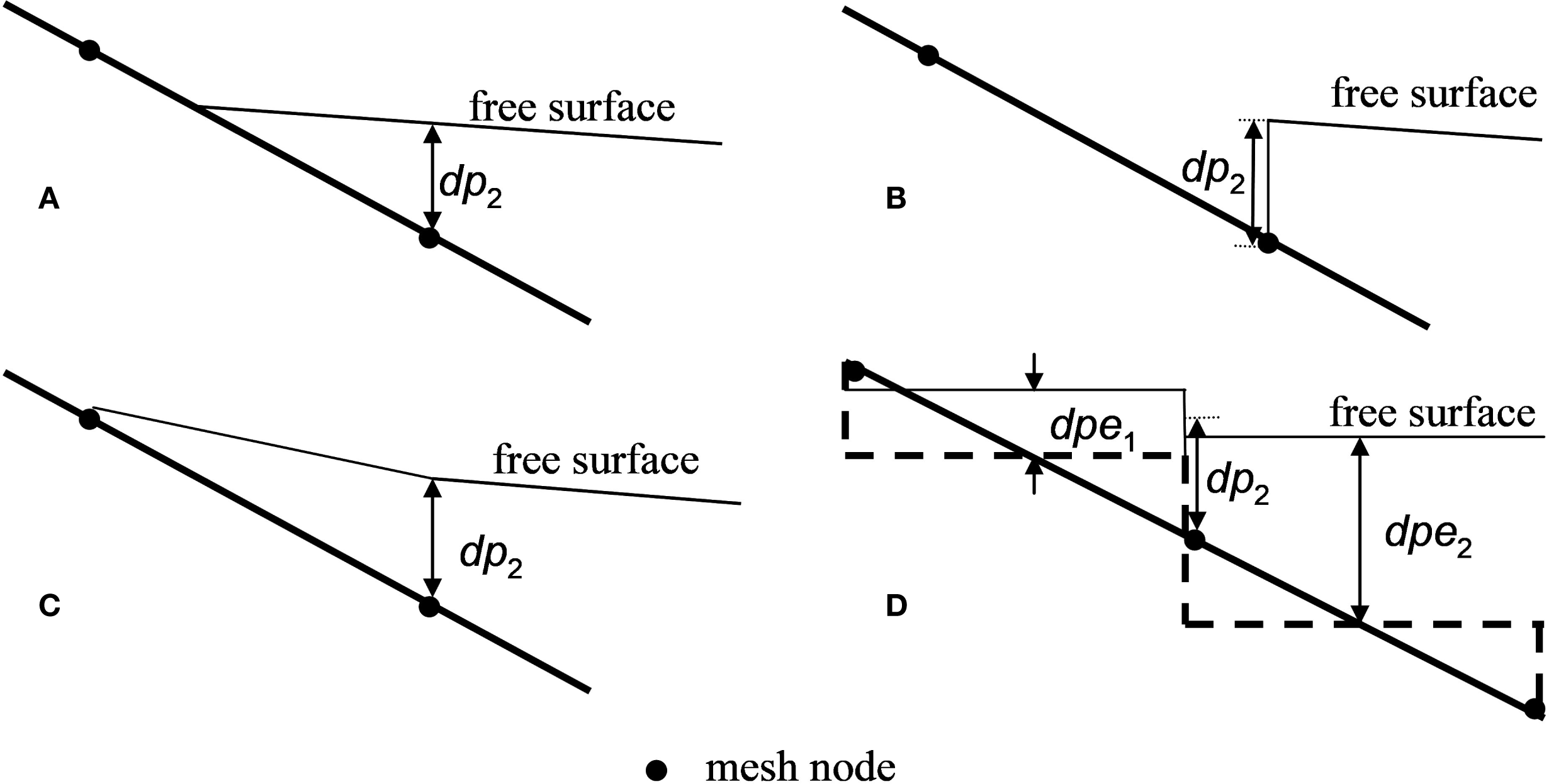
Representation of a continuous free surface in a finite-volume model based on a fixed grid: (A) partially wet (dry) element; (B) partially wet element excluded in the computation; (C) partially wet element included in the computation as approximated by previous methods; and (D) the discrete form of the region within the computational domain. Note that dp2 is the water depth of the wet node; dpe1 and dpe2 are the water depths of the partially wet and the fully wet elements, respectively.
Many studies have been conducted to improve the method by addressing the above-mentioned problems. Detailed comparisons between different fixed grid methods can be found in Balzano (Vacondio et al., 2014) and Horitt (Jafarzadegan et al., 2023). Sabbagh-Yazdi and Zounemat-Kermani (Sabbagh-Yazdi and Zounemat-Kermani, 2009; Yoshioka et al., 2014) added an artificial viscosity to the formulation to damp out the numerical oscillations caused by wetting and drying. Falconer and Chen (Falconer and Chen, 1991)improved the method by considering the direction of the flow velocity when determining whether or not a dry cell is becoming flooded. Liang and Marche (Liang and Marche, 2009) developed a 1D flow solver for simulating frictional flows over complex domains involving wetting and drying by ensuring the positivity of water depth and deriving additional source terms to balance spurious fluxes. Brufau et al. (Brufau et al., 2004) modified the wetting and drying condition by including the normal velocity to the cell edge to achieve high accuracy in mass conservation. Bunya et al. (Bunya et al., 2009) proposed an operator to keep the water depth positive to prevent numerical instability due to excessive drying. Bates and Hervouet (Bates and Hervouet, 1999; Bates, 2000) improved the method by rescaling the continuity equation on the basis of the sub-grid topography, identifying partially wetted elements on the basis of a simple analysis of water surface slopes and removing spurious water-surface slope terms in the momentum equation. Defina (Defina, 2000) defined a function to describe the wet area fraction of a partially wetted element. Based on this function, new momentum and mass balance equations were developed with consideration of local topographic variations to allow a realistic description of small water depth flows. Another class of fixed grid model, different from including or excluding partially wet cells from the computational domain, has got considerable success recently, which solve continuity (and scalar mass conservation) equations in all cells on a fixed grid, but only solve momentum equations in fully wetted cells (Bradford and Sanders, 2002; Begnudelli and Sanders, 2006). Bradford and Sanders (Bradford and Sanders, 2002) explored the benefits of extrapolating the velocity in to partially wetted cells which proved helpful in highly dynamic wave runup and rundown problems. This scheme was the basis of a more general purpose 2D flow and transport model which proved to be excellent for tracking sharp fronts in tidal wetlands (Begnudelli and Sanders, 2006). The Volume-Freesurface Reconstruction (VFR) method by Begnudelli and Sanders (Begnudelli and Sanders, 2006) distinguished between the volume in a cell and the free surface height in a cell, which allowed for a physically reasonable filling and draining of partially wetted cells and improved variable reconstruction at cell edges in support of mass and momentum flux calculations. Despite these developments, accurate simulations of moving WDF remains a difficulty in modelling shallow water systems, especially coastal wetlands where large areas undergo periodic wetting and drying under the influence of tides.
In this paper, we present a new algorithm for accurately and efficiently simulating the WDF as it moves along the sides of the partially wetted elements. The method tracks the WDF defined by zero water depth and flux. The movement of the WDF results in changes of the flow domain’s boundary as discussed above. Such changes occur within the partially wetted elements, where the wet area is partly bounded by the wetting and drying front. As the front moves, the attributes of these elements vary, including the wet fractions of sides (which intersect with the WDF) and area, and representative water depth. These quantities, computed every time step, are incorporated in the solution to reflect the influence of the moving WDF on the flow. In essence, this algorithm treats the partially wet cells as special fully wet cells by cell division method and solve momentum and continuity equations in both partially wet and fully wet cells. The rest of the paper is organized as follows: section 2 presents the mathematical model together with details of the numerical strategy and improved WDF tracking algorithm. Section 3 presents test cases. Finally, conclusions are made in section 4.
2 Mathematical model and numerical solution
2.1 Hydrodynamic model ELCIRC
A three-dimensional hydrodynamic model, ELCIRC (Zhang et al., 2004), was selected for studying the wetting and drying problem and implementing the new WDF algorithm. ELCIRC uses a finite-volume/finite-difference Eulerian-Lagrangian method to solve the shallow water equations. It has been used to simulate a wide range of physical processes in shallow water systems driven by atmospheric, ocean and river forces (Baptista et al., 2005; Zhang and Baptista, 2004; Gong et al., 2009; Wang et al., 2008). The numerical method is volume-conservative, stable and computationally efficient. The model incorporates the wetting and drying condition based on a traditional fixed grid method. In our study, we examined the suitability of ELCIRC for simulations of flow and transport in salt marsh systems. Salt marshes are important coastal wetlands where extensive areas are subjected to periodic wetting and drying as tides rise and fall. The existing wetting and drying algorithm within the ELCIRC model were found to be inadequate for proper simulations of the moving boundary due to wetting and drying, and its effects on flow and transport processes in these tidal wetland systems.
The detailed mathematical model of ELCIRC can be found in (Zhang et al., 2004). For the purpose of simplicity and clarity, here we take two-dimensional non-linear shallow water Equations 1–4 as the governing equations to illustrate the improved wetting and drying algorithm:
where , are the horizontal Cartesian coordinates and is the vertical coordinate [L]; is the time [T] and is the z-coordinate of a reference level [L] (e.g., mean sea level [L]); is the free surface elevation [L] and is the bathymetric depth [L]; , and are the water velocities in the , and direction, respectively [L/T]; g is the magnitude of the gravitational acceleration [L2/T]; is the fluid density [M/L3], is the base density [M/L3] is the vertical eddy viscosity [L2/T]; is the vertical eddy diffusivity for solute [L2/T]; is the atmospheric pressure at the free surface [M/LT2]. Note that wind stress and Coriolis force although not presented in the above governing equations for the purpose of simplicity, are integrated in the ELCIRC model.
For the bottom boundary, ELCIRC assumes a balance between the internal Reynolds stress (Equation 5) and the bottom frictional stress (Equation 6), i.e.,
with the bottom shear stress [M/L1T2] and [M/L1T2] defined as follows,
where [L/T] and [L/T] are the velocities at the bottom; and [-] is the bottom drag coefficient calculated according to with being the Manning coefficient [4].
2.2 Numerical solution with the existing wetting and drying algorithm
In ELCIRC, the computational domain is discretized into a combination of triangular and/or quadrangular elements in the horizontal plane. We suppose that in total, the mesh has nodes, elements and sides. Topography is defined by the still water depth (dp) specified at each node (x,y), i.e., . Organization of the neighborhood of elements, nodes and sides within the mesh is critical for unstructured grid-based models. Integer mapping arrays are used to define the neighborhood of nodes, sides and elements surrounding each other’s, as shown in Figure 2.
Figure 2
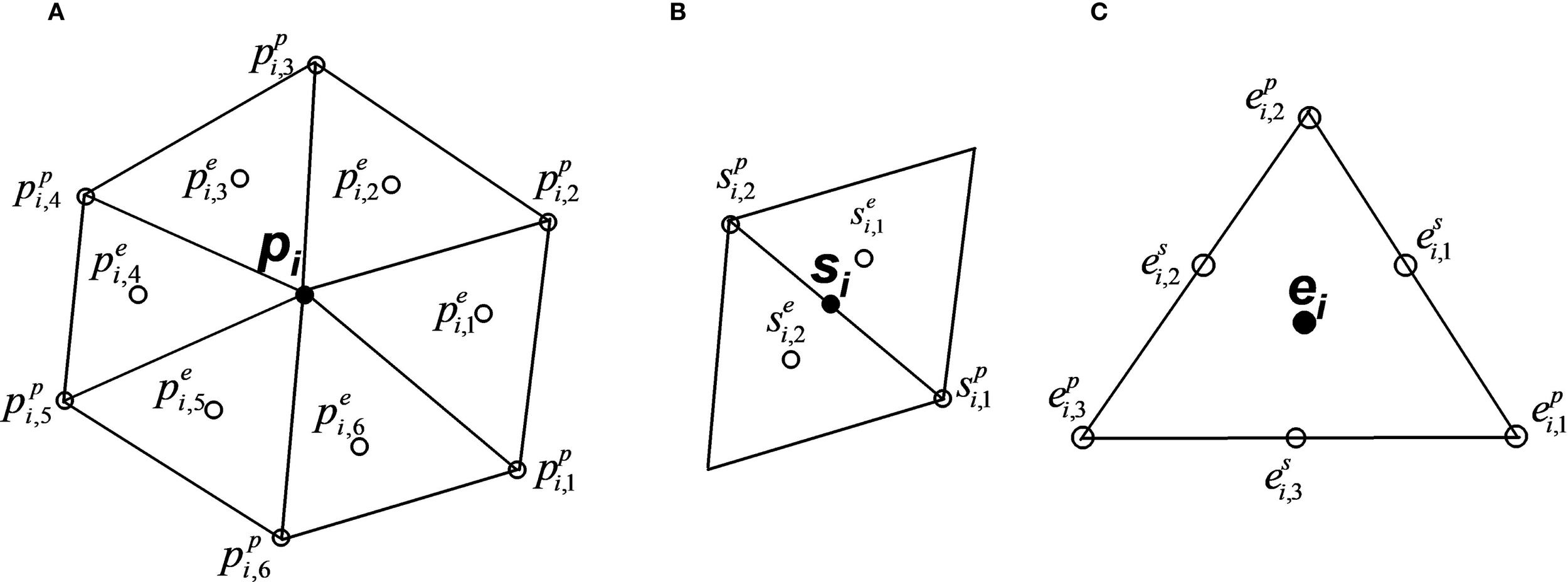
Schematic diagrams of the grid showing the neighborhood mapping for (A) node (indicated by circles), (B) side, and (C) element. The symbol indicates the object under consideration. The superscript indicates the nature of the neighbouring object – whether it is a node (p), side (s) or element (e). The subscript indicates the relationship between the object and its neighbouring objects.
Nodes surrounding node are mapped by and surrounding elements by , where and ; is the number of the nodes and elements that surround each node, typically in the range of 4-10. Similar notations apply to the mapping related to the side , including (for surrounding nodes) and (for surrounding elements), where and . Note that represents the length of the side and is the distance between the orthocentres of two elements that share side i. Considering the th element , the surrounding nodes and sides are and , where and j = 1,…, i3-4 (i3-4 = 3 or 4, depending on whether the element is triangular or quadrangular). Ai is the area of the element.
The existing wetting and drying algorithm used in ELCIRC is based on a traditional turn off/on method, which excludes partially wet elements from the computational domain. At the beginning of each time step, the wet/dry status of each node, side and element is determined. The mass conservation equation is solved for wet elements using the finite-volume method to obtain elementwise water levels (for the element orthocentre). The momentum conservation equations are solved for wet sides with the Eulerian-Lagrangian algorithm to obtain sidewise velocities (for the side’s midpoint). Then nodewise water level is calculated by interpolation. At a node (i) where all surrounding elements are wet, the nodewise water level is computed as an area-weighted average of the elementwise water levels (Equation 7), i.e.,
where is the number of wet elements surrounding the node and is the elementwise water level for kth wet element around the node. At a node surrounded by both wet and dry elements, its water level is computed based on a simple arithmetic average (Equation 8).
where kmax,w is the number of wet elements surrounding the node. Subsequently, the wet or dry status of each node is determined based on its water depth (h = η - Hs) relative to the threshold h0: wet if h ≥ h0 and dry if h<0. The status of the element is then updated according to its surrounding nodes. An element is wet only when all the surrounding nodes are wet. Similarly only sides with both end nodes wet are updated as wet sides. As mentioned in the introduction, this approach leads to an unrealistic representation of the motion of the wetting and drying front and causes problems such as violation of the mass conservation principle. Also it tends to be seriously affected by numerical oscillations.
2.3 Numerical solution with the improved wetting and drying algorithm
Studies have been conducted to examine how partially wet elements may be retained in the computational domain in order to improve the numerical solution. In dealing with the partially wet elements, previous methods re-distributed the water volume over the whole element area while maintaining the geometry of the elements (Horritt, 2002; Begnudelli and Sanders, 2006). In contrast, the present improved algorithm considers directly the movement of the WDF across the partially wet elements. As the WDF moves, the wet parts of sides and area of a partially wet element expand or contract. Such changes are tracked and their effects on the flow are incorporated in the numerical solution with the improved method.
Following previous studies (Horritt, 2002; Heniche et al., 2000; Begnudelli and Sanders, 2006; Lu et al., 2024), an inundation function is defined for a region with area . The inundation function takes the value of 1 for wet areas or wet sections of sides and 0 for dry areas or dry sections of sides (Figure 3A). Then the wet fraction of area for a partially wet element is defined as Equation 9:
Figure 3
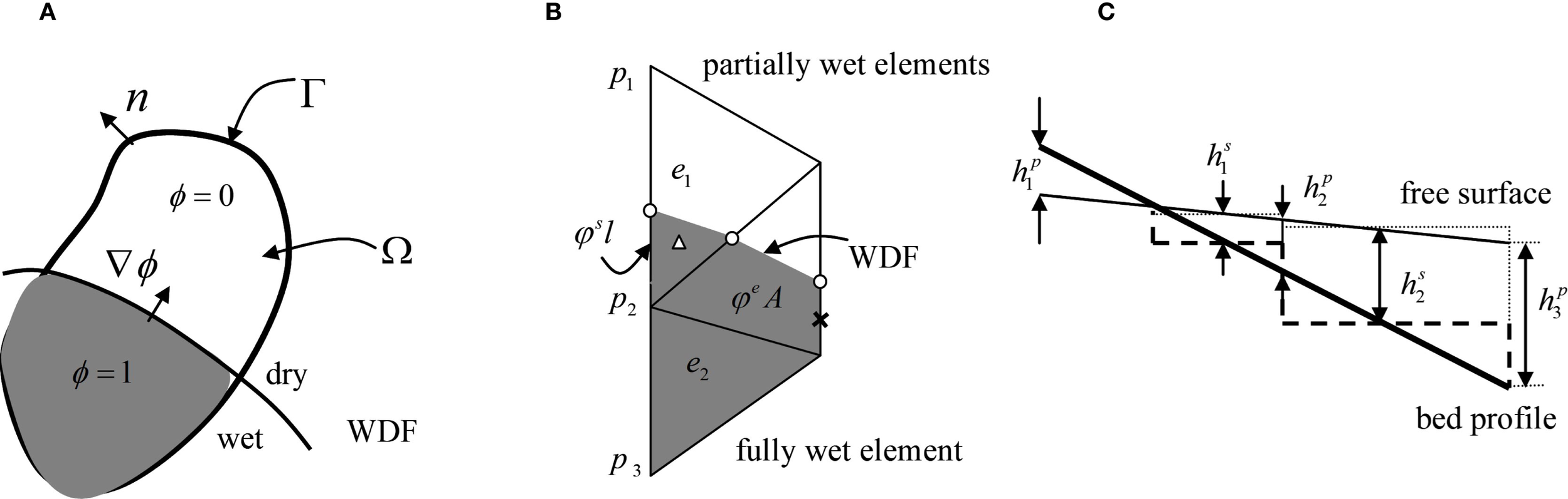
Schematic diagrams illustrating concepts and treatments used by the improved method: (A) a computational region bounded by the segment with normal unit vector . The function is the inundation function with value unity for wetted parts and zero for dry parts. Its gradient is perpendicular to the WDF; (B) discretization in the horizontal plane (x-y) with circles highlighting the intersections of the WDF with partially wet sides, a cross showing the midpoint of the wet part of a partially wet side and a triangle indicating the orthocentre of the wet part of a partially wet element; and (C) discretization in the vertical plane (x - z) with h1s indicating the water depth at the midpoint of the wet part of a partially wet side, which is used in computing the solution.
The wet fraction of side length is given by Equation 10:
where l is the length of the side.
Equation 8 is used to calculate the nodewise water level with being the total number of wet and partially wet elements surrounding the node. Based on the computed nodewise water levels, the status of nodes, elements and sides can then determine by Equations 9, 10. To locate the WDF, its intersection with a partially wet side, of zero water depth, is calculated by linear interpolation of water depth between the wet and dry nodes of the side. The WDF intersection points together with wet nodes form a wet triangle or quadrangle in a partially wet element, i.e., the wet part of the element. The partially wet element can then be treated as a wet element with new geometric parameters based on the wet part of the element (Figures 3B, C), including the element orthocentre and midpoints of sides.
A semi-implicit finite-volume approach is used to discretize the continuity equation. Following Casulli and Waters (Casulli and Walters, 2000) and Zhang et al. (Zhang et al., 2004), we constructed a local coordinate system based on an element side with the x-axis pointing outside of the element from the center of the side. Correspondingly, and represent normal and tangential velocities in the discretized equations. For element , the discretized continuity equation is given by:
where superscripts and denote the time steps, is time step, and is the weighting between time levels for the temporal discretization. The function assumes a value of 1 or -1 depending on whether the unit vector normal to the kth side of the element points outward or inward, respectively. Equation 11 applies to both wet and partially wet elements. Compared with previous numerical solutions, this equation includes two additional parameters to deal with partially wet elements: the wet fraction coefficients of element area () and sides (). Both coefficient values range between zero (completely dry) and unity (completely wet). When computing the flux terms in Equation 11 for a partially wet side, one must consider only the wet section of the side, i.e., u (local normal velocity) and h (local water depth), both based on the midpoint of the wet section. This approach is derived from considering continuity for a partially wet element only within the wet part of the element. Note that the flux across the totally dry side (part of the WDF) is zero because of the zero-water depth even though the calculated flow velocity at the side is non-zero.
The Eulerian-Lagrangian method is adopted to treat the convection terms of the momentum equations. Thus the discretized momentum equations are:
where and are the backtracked values obtained using the Lagrange reverse-tracing method (Casulli and Walters, 2000). Again when applied to partially wet elements, these equations are evaluated based on the wet parts of the elements. To solve the side-based discretized normal momentum equation, the distance between the orthocentres of two adjacent elements needs to be calculated; if a partially element is involved, its orthocentre is based on the wet part of the element. The tangential momentum Equation 12, applied to a side, involves the length of the side and the water surface elevations of its two end nodes for approximating the water surface slope (second term on the RHS of Equation 13). For a partially wet side, the side length is based on the wet section of the side, i.e., (φsili). This wet section has a dry node as given by the intersection with the WDF, where the water surface elevation equals the bed elevation. This allows more accurate predictions of the water surface slope in the partially wet element.
The WDF algorithm is summarized as follows:
-
Determine the status of nodes, sides and elements based on current nodewise water levels;
-
Determine the locations of WDF (intersections with partially wet sides) and wet parts of partially elements;
-
Update the geometric parameter values for partially wet elements (orthocentres of the wet part of the element) and sides (midpoint of the wet section of the side);
-
Calculate and for partially wet elements and sides;
-
Solve mass and momentum conservation equations for wet and partially wet elements to get elementwise water levels and sidewise velocities;
-
Interpolate computed elementwise water levels to get nodewise water levels;
-
Go back to the first step to start computation for next time step.
Compared with the existing wetting and drying algorithm used in ELCIRC, the improved algorithm presented here incorporates the partially wet elements in the computation. In particular, the current method tracks the movement of the WDF within these partially wet elements and deals with the wet parts of the elements, which evolve with moving WDF. In contrast to previous methods, this algorithm solves the continuity and momentum equations specifically for the wet parts of partially wet elements rather than seeking whole element-based solutions by approximations of water re-distribution in the elements (Defina, 2000). The method of decomposing physical processes is conducive to proposing approaches to solving complex problems (Gao et al., 2023, Gao et al., 2024).
3 Numerical tests
3.1 Comparisons with the traditional method originally used in ELCIRC
To compare the performance of the improved method with that of the traditional method, we applied both methods to simulate a simple case of flows on a tidal beach. The computation domain had a plan dimension of 6000 m × 2000 m with a bed slope 0.0005 (Figures 4A, B). Slip conditions were invoked at the lateral boundaries (y = -1000 and 1000 m). A still water with an elevation of 0 m was assumed as the initial condition; all the simulations were run for a sufficiently long period of time for the system to reach a quasi-steady state (i.e., periodic solution with the effect of initial condition diminished). An inflow boundary was imposed at the left-hand side (LHS) of the domain, where the time-varying water depth mimicking the tide was specified as:
Figure 4
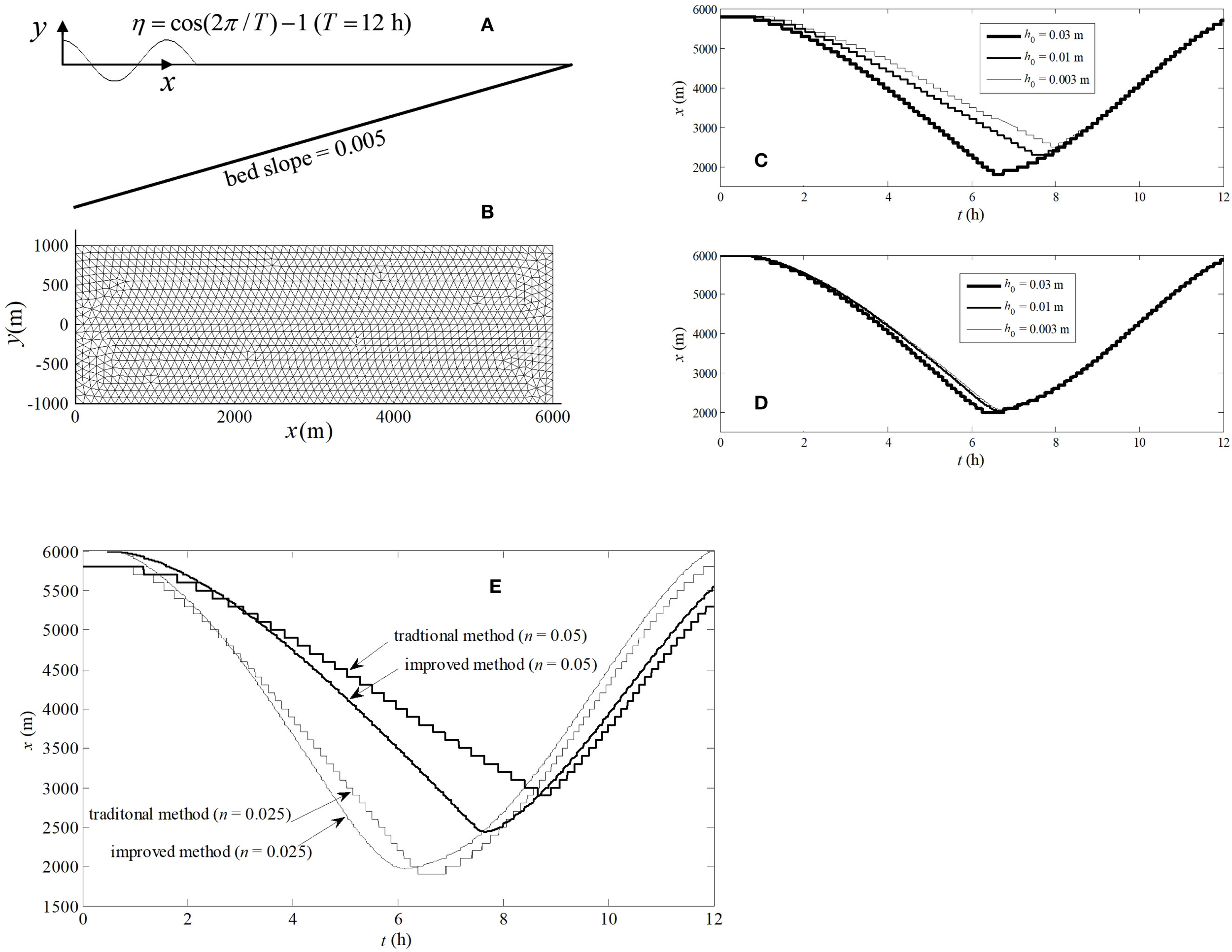
Topography (A) and mesh grid (B) for the first test case; Comparison of the wetting and drying fronts predicted by the traditional method (C) and the improved method (D) with different thresholds (h0) used in the simulations; Comparison of the wetting and drying fronts predicted by the traditional method and the improved method with different Manning coefficient (n) values used in the simulations (E).
where h is the period of the tidal cycle. The right-hand side (RHS) of the domain was assumed to be an impermeable boundary (no flux). The quasi-steady results from the test simulations are discussed below.
With the fixed-grid approach, setting a proper value for the critical water depth h0 (threshold for the wet-dry separation) is important and yet often arbitrary. Ideally the simulation results should be insensitive to h0 once it is set in a small-value range as required by the convergence of the solution. The first test was on such insensitivity. We compared the movements of the WDF predicted by the traditional and improved method in Figure 4B. The results show that the predictions by the traditional method varied significantly with . The predicted WDF moved more slowly when the threshold was set smaller. This is a numerical artefact that has been observed in previous numerical studies (Schubert et al., 2008). In contrast, the improved method gave predictions that were more or less independent of the threshold once its value was set small enough (Figure 4D).
We also tested how the improved method performs with different Manning coeddicent values. Figure 4E shows the comparison of the WDFs predicted by the traditional method and improved method with different bottom drag coefficient (Manning coefficient) values. When the Manning coefficient was small, the difference between the results given by these two methods is minor. However, their predictions started to deviate significantly as the Manning coefficient increased, especially during the falling tide. The reason which causes the difference is that the traditional method distributes the fluid volume all over the area of partially wet cell. When a partially wet cell will be dried soon, water only occupied a small part of its area. Using the whole area to divide fluid volume to get water depth is unreasonable and smaller than reality. As Equations 12 and 13 show, the last term contains water depth and Manning coefficient. The bigger Manning coefficient is, the more important the term including the water depth is in Equations 12 and 13, then the bigger error caused with the traditional method, the more difference the two methods show.
To further examine the performances of both methods, we calculated the accumulated mass errors of the simulations as given by the sum of differences between total water volume change in the domain and the net flux across the seaward boundary for the falling and rising tide periods (Table 1). These errors are associated with the artificial water loss (negative error) and gain (positive error) due to drying and wetting, respectively. It is important to point out that the errors for the two different tidal phases do not cancel each other and are likely to affect significantly the simulation of solute transport in the system (if it were considered), causing long-term mass imbalance problems. The comparison shows that the accumulated mass error in the prediction by the improved method is significantly smaller than that given by the traditional method. It is also evident from the results that smaller threshold helps to reduce the mass error in both cases. However, such a reduction can only be achieved meaningfully with the improved method because changes in h0 with the traditional method will lead to incorrect simulations of the WDF’s movement and flow in the adjacent, shallow water area as discussed above.
Table 1
| Tidal process | Mass error (×102 m3) (Traditional method) | Mass error (×102 m3) (Improved method) | |||
|---|---|---|---|---|---|
| H 0 = 0.03m | H 0 = 0.01m | H 0 = 0.03m | H 0 = 0.01m | H 0 = 0.001m | |
| During ebb tide | 8.2 | 6.8 | 4.0 | 1.4 | 0.8 |
| During flood tide | -1.8 | -1.0 | -1.2 | -0.8 | -0.6 |
Comparison of accumulated mass errors in the simulation results given by the traditional method and the improved method with different thresholds used in the simulations.
3.2 Moving shorelines over a frictional parabolic topography
Sampson (2006), Liang and Marche (2009) derived an analytical solution of the non-linear shallow water equations for perturbed flow in a container with a frictional bed of parabolic topography. This solution serves as a benchmark test for validating the wetting and drying procedure in the numerical model. The bed profile of the domain is defined by:
where and are constants. The analytical solution depends on a bed friction parameter (related to the bed friction coefficient according to ) and a hump amplitude parameter ,
where is the water surface elevation above the bed’s lowest point (datum), is a constant that corresponds to a specified initial condition and . As , , being the still water elevation above the datum. The projection of the WDF (two parallel straight lines on the plane) is given by
As , , indicating that the oscillatory flow is completely damped by bed friction.
In the numerical simulation, the computational domain had plan dimensions of 10000 m (x) 1000 m (y). Slip conditions were invoked at the lateral walls. The following parameter values in Equation 15 were used: km, m, and . The numerical simulation lasted for 6000 s. Figure 5 shows the comparisons between the numerical predictions and analytical solutions of the free water surface profile at various times throughout the simulation. The moving WDFs on both sides and the water surface were well reproduced by the improved method at all times. This is in contrast with the rather poor performance by the traditional method. At t = 6000s, the WDFs predicted by the improved method coincide with the analytical solution (Equation 17). In contrast, due to volume loss, the WDFs obtained by the traditional method are lower. The improvement by the current method is further demonstrated in Figure 6 where the time-varying surface elevation at two locations and Figure 5 where the time-varying WDF at the left side are shown. Figure 6 shows that both the amplitude of local water level oscillations and the asymptotic water level have been under-predicted by the traditional method. The current method improved the numerical simulation in both aspects. Error curves (Figure 6C) are computed to qualify the accuracy of the numerical predicts. The error is defined as
Figure 5
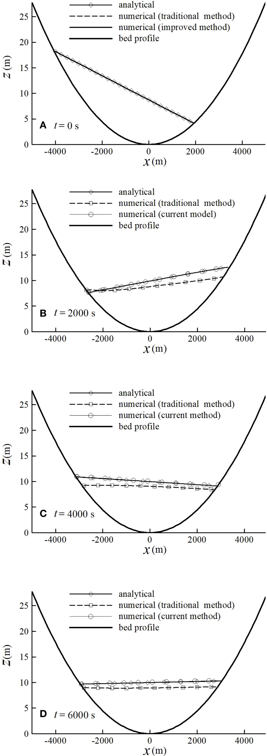
Sloshing motions in a vessel with a parabolic bottom topography (Equation 15), as predicted by the analytical solution (Equation 16) and numerical simulations at (A)t=0 s, (B)t=2000 s, (C)t=4000 s and (D)t=6000 s.
Figure 6
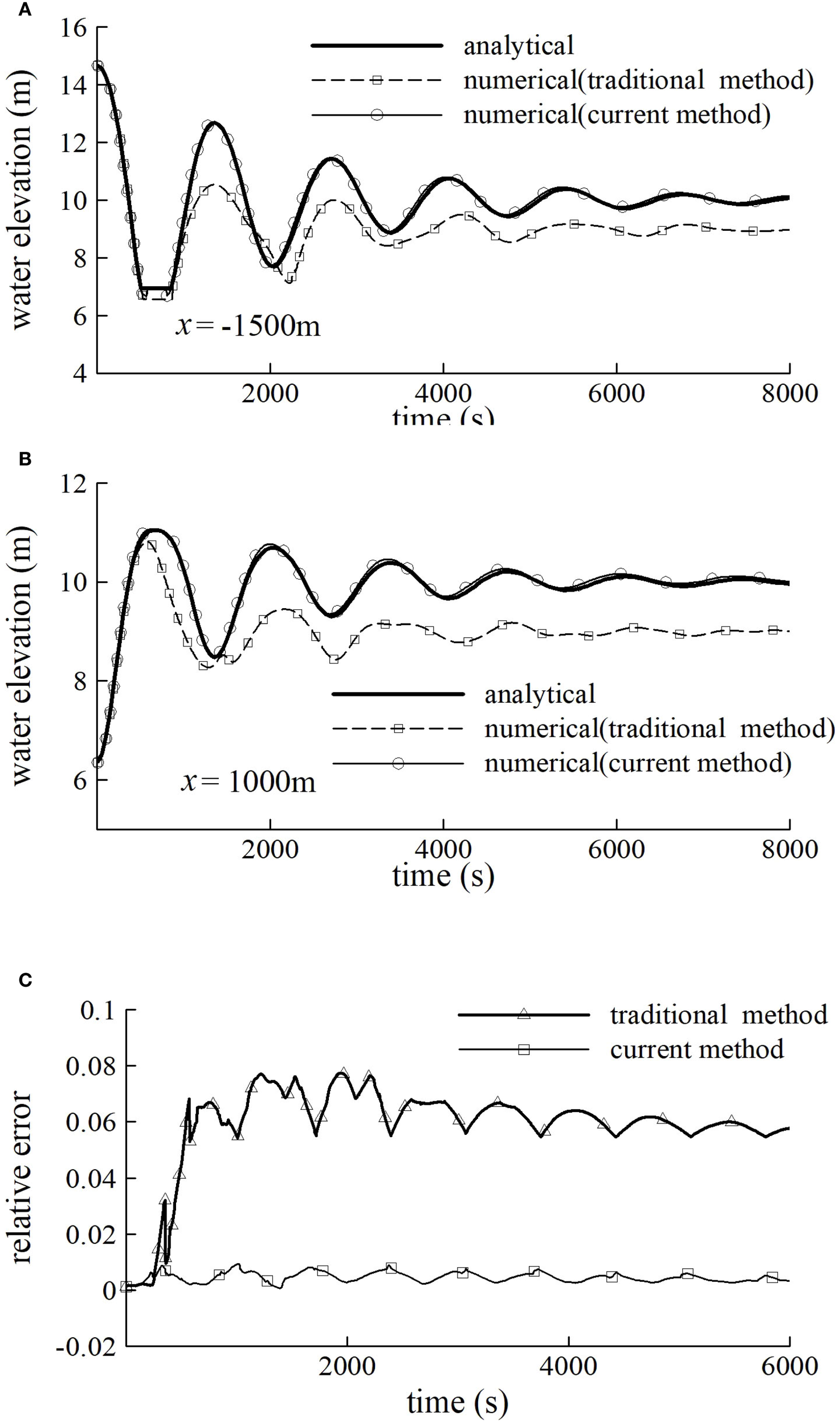
Water surface elevation varying with time at (A) point (-1500, 0) and (B) point (1000, 0), as predicted by the analytical solution (Equation 16) and numerical simulations, and (C) the error time history with the traditional method and current improved method.
where ηi and zsi are the predicted and analytical water surface elevation at cell i. Figure 6C presents the error time history of error for the simulations on the grid with 100 cells. With same grid and time step, the error is found about 0.005 with current mothed and 0.06 with traditional method. Figure 5 shows that the predicted WDF with current method matches considerate well with analytical solution while with traditional method, error is more and more serious with time going on. When a point becomes dry, the speed of the flow at the point is as same as the speed of WDF at that time. The speed of the WDF of this case could be computed from Equation 16. Then we choose two points to compare their speeds predicted by traditional method, current method and analytical solution. Figures 6A, B present that better results, no matter about the transient time when the points dried or the speed during the points drying, could be got by current method.
3.3 Tidal flow on a beach with variable slope
A further test was conducted to examine predictions of the WDF movement driven by tides on a beach with a non-uniform slope. The computational domain was set to be 500 m long in the x direction. The bed elevation was defined by Equation 18:
A still water level with an elevation of 0.35 m was used as the initial condition. The inflow boundary was imposed at the RHS of the domain, where the time-varying water depth driving the tidal cycle was specified as Equation 19:
where min is the period of the simulated tide. The LHS of the domain was assumed to be an impermeable boundary. A constant Manning coefficient of 0.03 was used throughout the domain. The predicted water surfaces by both the traditional method and the improved method at four different times are compared in Figure 7. As the tide receded, the water surface elevation decreased gradually across the simulation domain. A very shallow water depth first occurred at (Figure 7A) around m where the bed slope changed from -0.001 to -0.01. It appeared that two flow regimes developed around the slope break point. Upstream of this point, the water was moving more slowly due to the gentle bed slope while the flow downstream retreated more rapidly because of the steeper bed slope. In principle, these two parts should not be separated totally. The slowly moving water upstream would continue to flow downstream. However, the result predicted by the traditional method (Figure 7B) exhibited flow separation, which was confirmed by the results of active elements shown in Figure 8B. In contrast, the improved method predicted a single connected water body with a gradually falling water surface and WDF, as physically expected (Figures 7A, B, 8A). While disconnected flows can occur in reality due to topographic depressions, the flow separation predicted by the traditional method in this case was a numerical artefact, which would further affect the mass transport if it was also simulated. From (Figure 7C), the shoreline moved up on the sloping beach slowly until the whole domain was submerged. The results predicted by the improved method for the rising tide stages agree closely with those reported in literature (Heniche et al., 2000), where a different numerical scheme was used. In particular, the problem with the slow movement of the WDF predicted by the traditional method, which caused over-steepening of the front (at t = 54 mins) (Figure 7D), was avoided by the improved method.
Figure 7
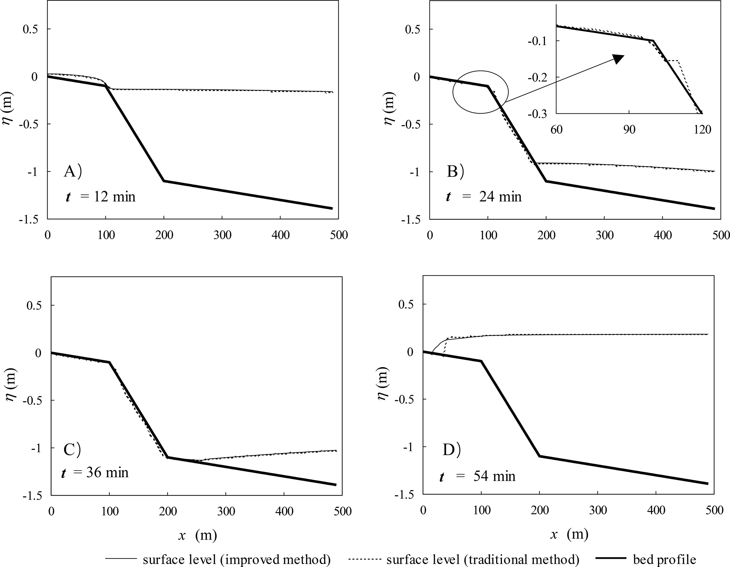
Tidal propagation on a beach with varying slopes defined by Equation 18: free surface elevation at four different times: (A)t=12 min, (B)t=24, (C)t=36 min, (D)t=36 min. Surface elevation at 500m is defined by Equation 19.
Figure 8
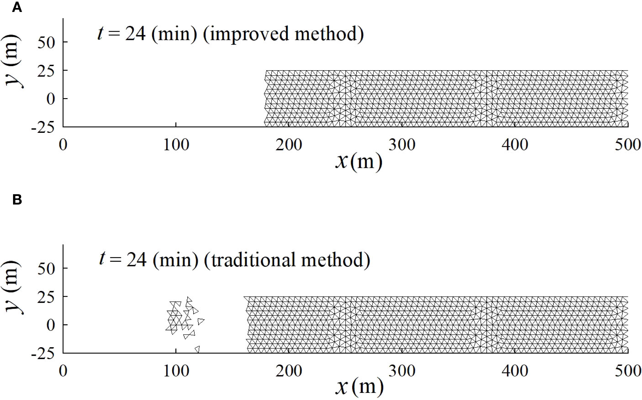
Tidal propagation on a beach with varying slopes: wet elements at t = 24 min (other areas of the domain are dry elements) with (A) improved method and (B) traditional method.
3.4 Application to a salt marsh system
In an estuarine channel or a salt marsh creek, the tidal flow asymmetry, sediment transport and morphology are interconnected. When the tide from deep water enters a shallow water body, transformations occur in its amplitude and shape. These transformations introduce distortions in the tidal wave form, both in the elevation and velocity time series. The interaction of tide with the bed and resulting transformations can be explained based on the nonlinear terms in the conservation equations of mass and momentum (Lanzoni and Seminara, 1998; Sivakholundu et al., 2009). Tidal fluctuations play a key role in plant zonation through alteration of soil aeration and salt transport, and drive the export of significant fluxes of carbon and nutrients to coastal water (Xin et al., 2022). We applied the improved method to study the different behaviors of residual sediment transport caused by different forms of tidal signals. The results explained to some extent why salt marsh systems tend to have diverse topographic structures.
For the purpose of computational efficiency, we first computed the propagation of tides in a tidal channel and subsequently used predicted local tidal signals of different forms at different locations to simulate their further propagation through the adjacent wetland systems such as salt marshes. The simulated channel had plan dimensions of 50 km (x) 500 m (y), a bottom slope of 0.0002 with a Manning coefficient of 0.02 (Figure 9B). The initial water level in the domain was set to be 1 m above the averaged mean sea level and the tidal forcing was specified at the origin of the x coordinate. The time series of water surface elevation and flow velocity became periodic after 4 tidal periods. Figure 10A displays the simulated temporal variations of water surface elevation at four different locations (P1 to P4) as shown in Figure 9A. The shape and phase of the tidal wave changed gradually from P1 to P4. Since our focus was on the shape of the driving tidal signal, the simulated tides at P2, P3 and P4 were shifted and rescaled to have the same phase and amplitude of oscillations, and phase-averaged value as those of the tide at P1 (Figure 10B) prior to their applications to the sub-scale (local-scale) models (Figure 9B).
Figure 9
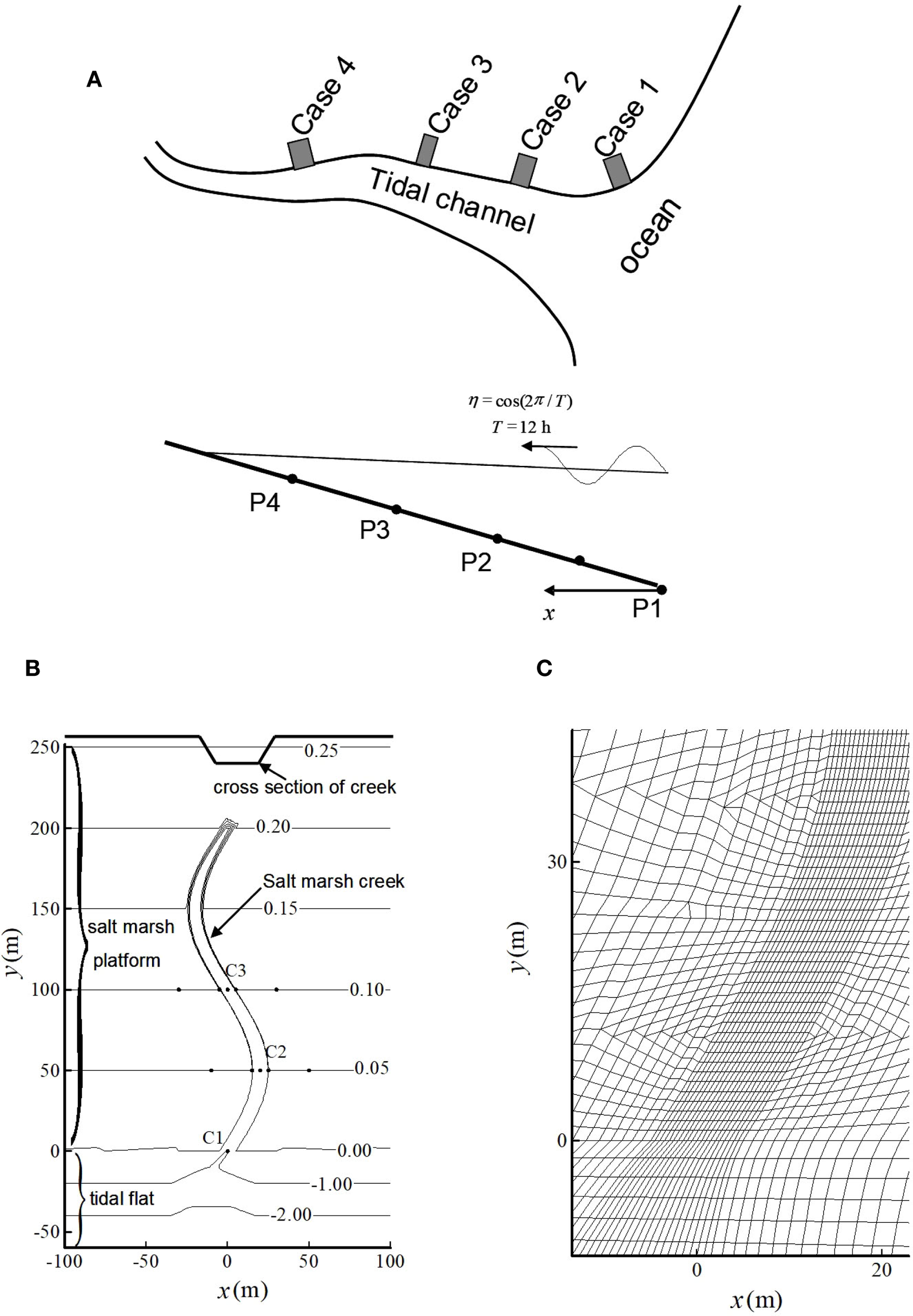
(A) Schematic diagram of the hybrid model consisting a large-scale tidal channel sub-model and four local-scale salt marsh models at points 1, 2, 3 and 4 along the channel (P1 is the origin of the x coordinate, P2, P3, P4 are 12.5 km, 25 km and 37.5 km inland of P1); (B) Schematic diagram of the local-scale salt marsh model with a meandering creek. The contours show the bed elevations in m; (C) Computational grid. High grid densities are needed near the creek to resolve the rapid topography changes.
Figure 10
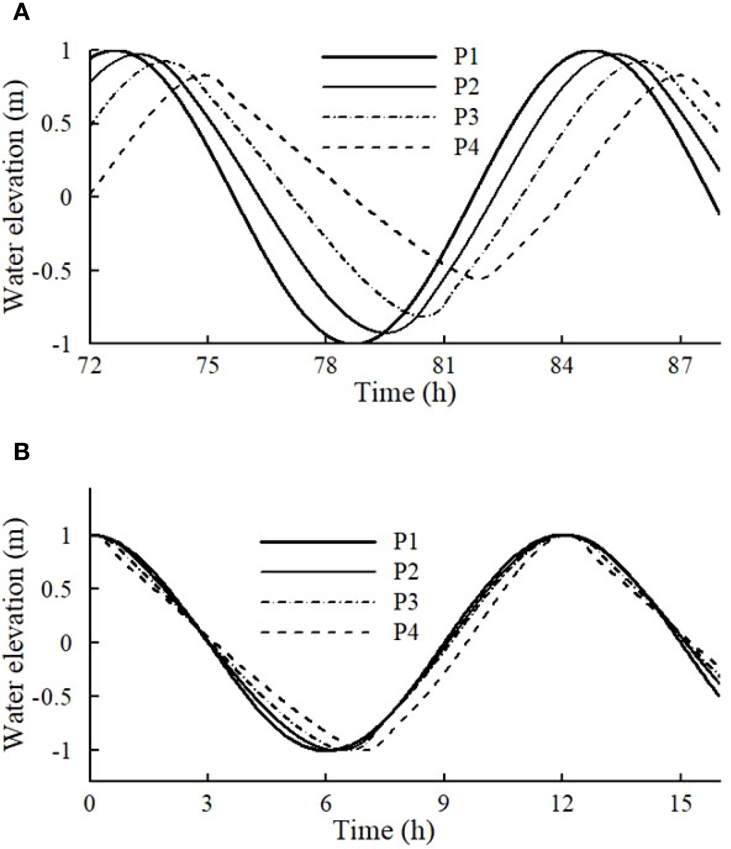
(A) Time serials of local water surface elevations at P1-P4; (B) Shifted and re-scaled tidal signals with the same phase, oscillation range and averaged elevation.
The modified tidal oscillations at P1-P4 were used as inputs for four local-scale salt marsh models to examine how four different forms of tides influence the tidal water flows and sediment transport in the wetland system associated with the tidal channel. The computational domain of the local-scale model was composed of a salt marsh platform of 250 m × 100 m in plan dimensions, and with a bottom slope of 0.001 and a Manning coefficient of 0.05. A tidal channel was assumed to border the marsh platform with a tidal flat of 60 m × 100 m in plan dimensions, a bottom slope of 0.05 and a Manning coefficient of 0.025. The tidal flat intersected the marsh platform at where both bed elevations were zero. A meandering creek was embedded in the salt marsh from m to m. The centerline of the creek followed a curve defined by the function . Along this centerline, the bed elevation of the creek varied from -1 m to 0 m linearly. The creek’s cross-section was assumed to be a trapezoid with the bottom side length equal to 2 m and the top side length 12 m. At the upper end of the creek, a bevel side was assumed with the same slope as that of the bevel side of the cross section. The Manning coefficient for the creek bed was assumed to be the same as that of the tidal channel bed, 0.025. Three observation points (C1, C2 and C3) were set along the creek’s centerline with y equal to 0, 50 and 100 m, respectively. Two other groups of observation points were also included in analyzing the simulation results: eight points with the same y coordinates as those of C2 and C3, and located symmetrically on both sides of the creek with distances of 5 m and 30 m away from the creek’s centerline (i.e., C2L1, C2R1, C2L2, C2R2, C3L1, C3R1, C3L2 and C3R2 shown in Figure 9B). The computational domain was discretized into a combination of triangular and quadrangular elements with the smallest length of the sides equal to 3 m (Figure 9C).
For the purpose of comparison, the first case (using the tidal signal at P1 as the driving force) was also simulated using the traditional method. Figure 11B shows that the wetting and drying front predicted by the traditional method was rather irregular. There were pockets of dry elements surrounded by wet elements at the creek bank and marsh platform. This phenomenon again is a numerical artefact as discussed in section 3.3. In contrast, these irregularities and artefact did not occur in the simulation using the improved method (Figure 11A). The improvement made by the improved method was further demonstrated by the results shown in Figure 11C which plots the speed of local tidal current at C2L1 during the drying period on a falling tide. The traditional method predicted a prolonged drying process during the falling tide due to the method’s over-prediction of the bed friction effect in the shallow water area near the WDF as discussed previously. The simulation by the traditional method further suffered large numerical oscillations associated with the drying process. The improved method clearly has resolved these problems and provides a feasible means for conducting the following analysis.
Figure 11
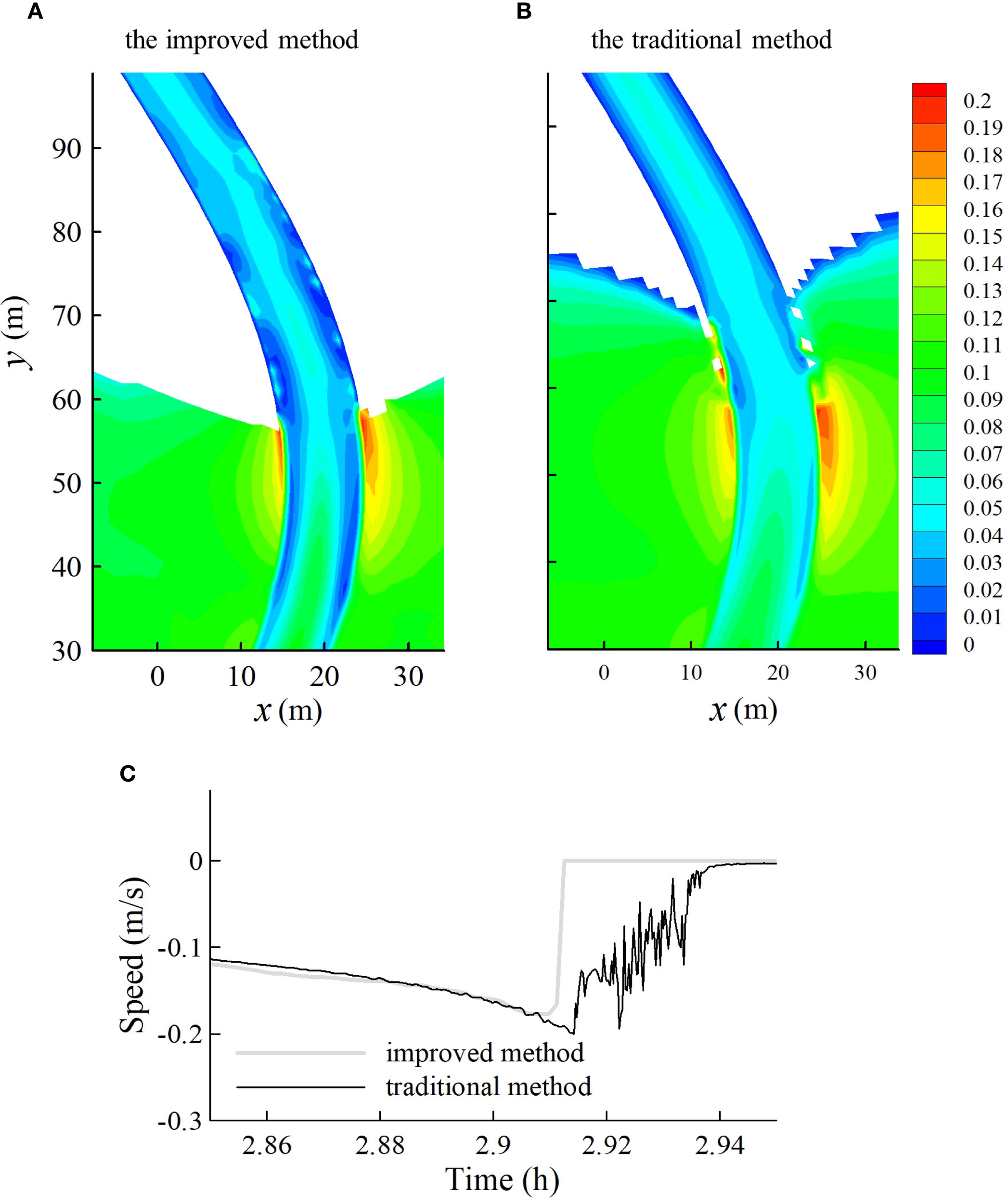
Comparison of the magnitude of the velocity (m/s) and the WDF predicted by the improved method (A) and the traditional method (B) for case 1; Comparison of the velocity of the tidal flow during the drying period during the falling tide at point C2L1 predicted by the improved method and the traditional method for case 1 (C).
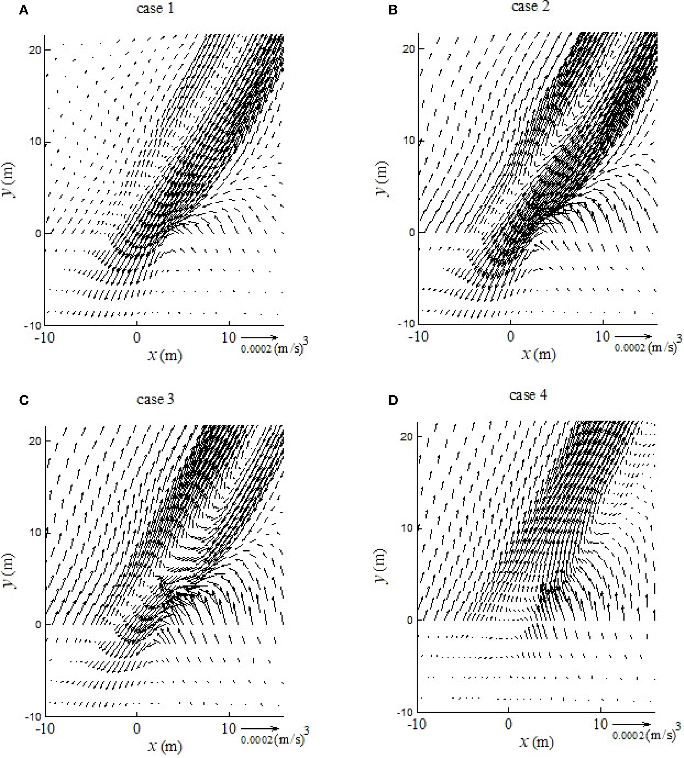
Salt marsh systems embedded with meandering creeks are complex systems involving many hydrodynamic processes. Here we illustrate this using a simplified model of sediment transport. The sediment transport rate () due to water current (neglecting threshold velocity for initiation of particle movement) may be expressed by , where is a function representing sediment grain size, bed slope characteristics, etc.; is current velocity; and varies between 2 and 5. We defined a net flux quantity over a tidal cycle, which might be related to the net (residual) sediment transport rate (Ip et al., 1998),
The divergence of this pseudo residual sediment flux was calculated to illustrate how the topography might change under different tidal signals (Figure 12). A positive divergence of the residual sediment flux indicates local erosion and a negative value is linked to local accretion. Figure 12 shows three trends of topographic variations as the tidal signal changed from P1 to P4: (1) the condition of the salt marsh platform changed from mainly stable to being accreted; (2) around the edge of the salt marsh platform and tidal channel, conditions changed from being accreted to being eroded; and (3) overall the creek remained eroded and the bank of the creek being accreted to different extents under all tidal signals.
Figure 12
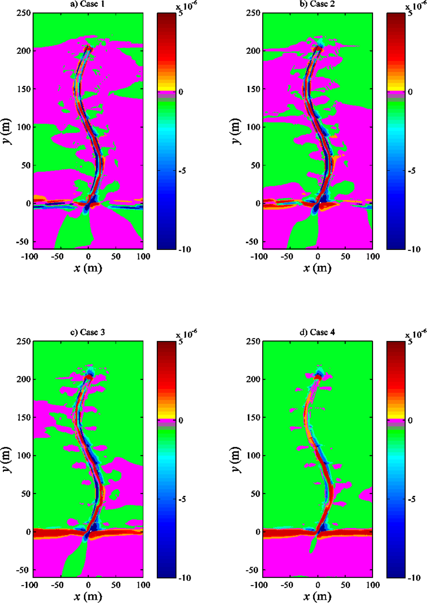
Spatial variations of divergence of pseudo residual sediment transport flux (m2/s3) for cases 1 (A), 2 (B), 3 (C) and 4 (D). The pseudo residual sediment transport flux is defined by Equation 20.
The topographic variations among the four cases were essentially due to the differences in the shapes of the tidal signals used to drive the models. Figure 13 shows the temporal variations of velocity at the observation points for case 1 and case 4. It is evident that the lengths of the flooding and ebbing tide periods differed between these two cases. The ebb tide in case 4 lasted much longer than that in case 1. Although local tidal signals of water surface elevation had the same amplitude in both cases (Figure 10B), the amplitudes of local velocity oscillations were different (Figure 13). Furthermore, the effect of topography on the flow velocity was significant, especially around the locations near the tidal creek. Flow directions at locations near the tidal creek varied from being predominantly perpendicular to the creek at the beginning of flooding and the end of drainage of the marsh platform, to being largely parallel to the creek for the rest of the rising and ebbing tide periods, respectively. The effects of topography on flow velocity and hence sediment transport rate is further shown in Figure 14. The spatial distribution of the residual sediment flux varied significantly with topography. Large spatial gradients of typically occurred at locations with rapid topographic changes, which would lead to large modifications of the local topography. Such flow-topography interactions underpin the evolution of the salt marsh and present a great challenge for numerical modelling. The challenge is two-fold: (1) in such a tidally influenced system, the residual flow and transport properties, which control the system’s long-term behavior, are likely to be controlled by higher-order processes, thus requiring highly accurate numerical solutions; and (2) topography variations, while representing a key driving factor of the system, exacerbate the problem with the WDF, hindering accurate simulations of the moving boundary.
Figure 13
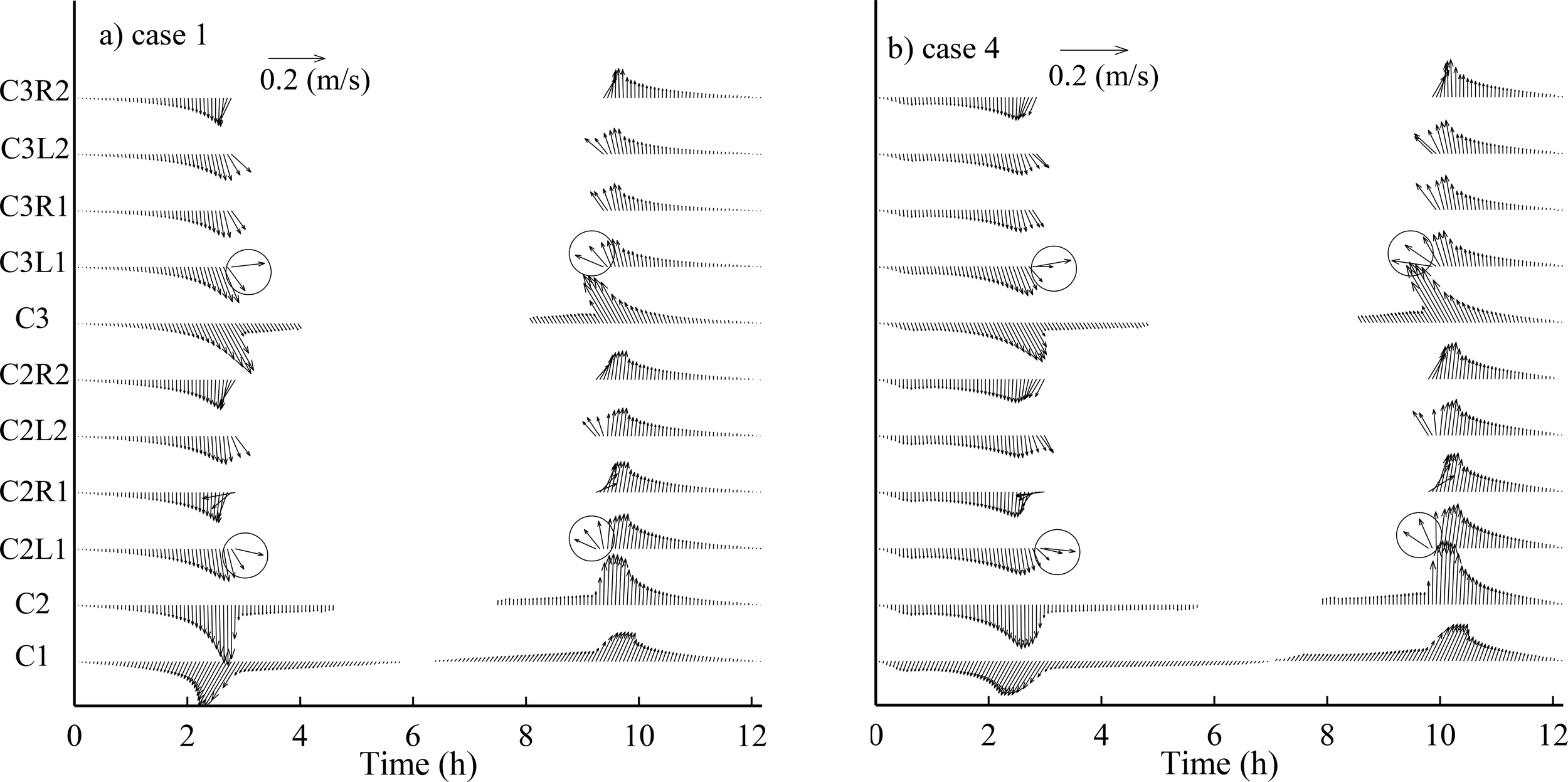
Temporal variations of flow velocity at different locations for case 1 (A) and case 4 (B). The ordinate of Figure (B) is identical to that of Figure (A). Circles highlight flows at locations near the tidal creek at the beginning of flooding and the end of drainage of the marsh platform with directions being predominantly perpendicular to the creek.
Figure 14
Pseudo residual sediment transport flux (q) near the creek mouth for cases 1 (A), 2 (B), 3 (C) and 4 (D).
The application case presented above has demonstrated the advancement made by the improved method in resolving these challenges, which will improve the capacity of hydrodynamic models for simulating complex flow and transport processes in coastal wetlands. The results suggested that (1) the numerical problems with the WDF encountered by the traditional method have been largely resolved by the improved method; and (2) particularly with the removal of numerical oscillations suffered by the traditional method, the improved method may be used to simulate and analyze high-order processes and quantities such as residual sediment transport flux, which control the evolution of coastal wetlands.
4 Conclusions
We have developed an improved wetting and drying algorithm for a hydrodynamic model based on unstructured grids. The algorithm combines an inundation function, wet fraction of area and wet fraction of side length to describe the changes of geometric parameters of partially wet elements with the moving WDF. These changes are fully incorporated in the numerical solution. The discretized continuity equation and momentum equations are solved for partially wet elements and sides with full consideration of the WDF movement to guarantee that local water surface slope, flux volume and bed friction are modelled accurately.
The test and application cases demonstrated the improvement achieved by the improved method in terms of mass conservation, and proper simulations of the WDF and bed friction effects in the near-front area. Moreover, the improved method has been shown to be capable of simulating high-order processes in a tidally influenced wetland system. Such simulations would not be possible with the traditional method, affected by numerical oscillations caused by the WDF movement.
Although it was implemented within a finite-volume model, the improved algorithm, in principle, can be applied to hydrodynamic models based on other numerical methods. The capability of this method will enable applications of numerical models to examine key processes that control the evolutions of coastal wetlands such as salt marshes.
Statements
Data availability statement
The original contributions presented in the study are included in the article/supplementary material. Further inquiries can be directed to the corresponding author/s.
Author contributions
LY: Conceptualization, Investigation, Software, Data curation, Visualization, Validation, Formal Analysis, Methodology, Writing – original draft, Writing – review & editing.
Funding
The author(s) declare financial support was received for the research and/or publication of this article. This research was supported by the National Natural Science Foundation of China [grant numbers 42276169].
Conflict of interest
The authors declare that the research was conducted in the absence of any commercial or financial relationships that could be construed as a potential conflict of interest.
Generative AI statement
The author(s) declare that no Generative AI was used in the creation of this manuscript.
Any alternative text (alt text) provided alongside figures in this article has been generated by Frontiers with the support of artificial intelligence and reasonable efforts have been made to ensure accuracy, including review by the authors wherever possible. If you identify any issues, please contact us.
Publisher’s note
All claims expressed in this article are solely those of the authors and do not necessarily represent those of their affiliated organizations, or those of the publisher, the editors and the reviewers. Any product that may be evaluated in this article, or claim that may be made by its manufacturer, is not guaranteed or endorsed by the publisher.
References
1
Baptista A. M. Zhang Y. L. Chawla A. Zulauf M. Seaton C. Myers E. P. et al . (2005). A cross-scale model for 3D baroclinic circulation in estuary-plume-shelf systems: II. Application to the Columbia River. Continental Shelf Res.25, 935–972. doi: 10.1016/j.csr.2004.12.003
2
Barros M. L. C. Da Silva T. D. Da Cruz A. G. B. Rosman P. C. C. (2020). Numerical simulation of wetland hydrodynamics and water quality. J. Braz. Soc. Mechanical Sci. Eng.42, 444–459. doi: 10.1007/s40430-020-02523-y
3
Bates P. D. (2000). Development and testing of a subgrid-scale model for moving-boundary hydrodynamic problems in shallow water. Hydrological Processes14, 2073–2088. doi: 10.1002/1099-1085(20000815/30)14:11/12<2073::AID-HYP55>3.0.CO;2-X
4
Bates P. D. Hervouet J. M. (1999). A new method for moving-boundary hydrodynamic problems in shallow water. Proc. R. Soc. London Ser. a-Mathematical Phys. Eng. Sci.455, 3107–3128. doi: 10.1098/rspa.1999.0442
5
Begnudelli L. Sanders B. F. (2006). Unstructured grid finite-volume algorithm for shallow-water flow and scalar transport with wetting and drying. J. Hydraulic Engineering-Asce132, 371–384. doi: 10.1061/(ASCE)0733-9429(2006)132:4(371)
6
Bradford S. F. Sanders B. F. (2002). Finite-volume model for shallow-water flooding of arbitrary topography. J. Hydraulic Engineering-Asce128, 289–298. doi: 10.1061/(ASCE)0733-9429(2002)128:3(289)
7
Brufau P. Garcia-Navarro P. Vazquez-Cendon M. E. (2004). Zero mass error using unsteady wetting-drying conditions in shallow flows over dry irregular topography. Int. J. Numerical Methods Fluids45, 1047–1082. doi: 10.1002/fld.729
8
Bunya S. Kubatko E. J. Westerink J. J. Dawson C. (2009). A wetting and drying treatment for the Runge-Kutta discontinuous Galerkin solution to the shallow water equations. Comput. Methods Appl. Mechanics Eng.198, 1548–1562. doi: 10.1016/j.cma.2009.01.008
9
Casulli V. Walters R. A. (2000). An unstructured grid, three-dimensional model based on the shallow water equations. Int. J. Numerical Methods Fluids32, 331–348. doi: 10.1002/(SICI)1097-0363(20000215)32:3<331::AID-FLD941>3.0.CO;2-C
10
Choudhary G. K. Trahan C. J. Pettey L. Farthing M. Berger C. Savant G. et al . (2025). Strongly coupled 2D and 3D shallow water models: theory and verification. J. Hydraulic Eng.151 (1), 04024049-1~14. doi: 10.1061/JHEND8.HYENG-13631
11
Defina A. (2000). Two-dimensional shallow flow equations for partially dry areas. Water Resour. Res.36, 3251–3264. doi: 10.1029/2000WR900167
12
Falconer R. A. Chen Y. (1991). An improved representation of flooding and drying and wind stress effects in a two-dimensional tidal numerical model. Proc. Institution Civil Engineers91, 659–678. doi: 10.1680/iicep.1991.17484
13
Gao J. Hou L. Liu Y. Shi H. (2024). Influences of bragg reflection on harbor resonance triggered by irregular wave groups. Ocean Eng.305, 117941–117961. doi: 10.1016/j.oceaneng.2024.117941
14
Gao J. Shi H. Zang J. Liu Y. (2023). Mechanism analysis on the mitigation of harbor resonance by periodic undulating topography. Ocean Eng.281, 114923–114942. doi: 10.1016/j.oceaneng.2023.114923
15
Ghazizadeh M. A. Mohammadian A. Kurganov A. (2020). An adaptive well-balanced positivity preserving central-upwind scheme on quadtree grids for shallow water equations. Comput. Fluids208, 104633–104653. doi: 10.1016/j.compfluid.2020.104633
16
Gong W. P. Shen J. Cho K. H. Wang H. V. (2009). A numerical model study of barotropic subtidal water exchange between estuary and subestuaries (tributaries) in the Chesapeake Bay during northeaster events. Ocean Model.26, 170–189. doi: 10.1016/j.ocemod.2008.09.005
17
Heniche M. Secretan Y. Boudreau P. Leclerc M. (2000). A two-dimensional finite element drying-wetting shallow water model for rivers and estuaries. Adv. Water Resour.23, 359–372. doi: 10.1016/S0309-1708(99)00031-7
18
Horritt M. S. (2002). Evaluating wetting and drying algorithms for finite element models of shallow water flow. Int. J. Numerical Methods Eng.55, 835–851. doi: 10.1002/nme.529
19
Ip J. T. C. Lynch D. R. Friedrichs C. T. (1998). Simulation of estuarine flooding and dewatering with application to Great Bay, New Hampshire. Estuar. Coast. Shelf Sci47, 119–141. doi: 10.1006/ecss.1998.0352
20
Jafarzadegan K. Moradkhani H. Pappenberger F. Moftakhari H. Bates P. Abbaszadeh P. et al . (2023). Recent advances and new frontiers in riverine and coastal flood modeling. Rev. Geophysics61. doi: 10.1029/2022RG000788
21
Johnsgard H. (1999). A numerical model for run-up of breaking waves. Int. J. Numerical Methods Fluids31, 1321–1331. doi: 10.1002/(SICI)1097-0363(19991230)31:8<1321::AID-FLD927>3.0.CO;2-K
22
Lanzoni S. Seminara G. (1998). On tide propagation in convergent estuaries. J. Geophysical Research-Oceans103, 30793–30812. doi: 10.1029/1998JC900015
23
Liang Q. H. Borthwick A. G. L. (2008). Adaptive quadtree simulation of shallow flows with wet-dry fronts over complex topography. Comput. Fluids38, 221–234.
24
Liang Q. H. Marche F. (2009). Numerical resolution of well-balanced shallow water equations with complex source terms. Adv. Water Resour.32, 873–884. doi: 10.1016/j.advwatres.2009.02.010
25
Lu L. J. Chen Y. C. Li M. J. Zhang H. Liu Z. W. (2024). Robust well-balanced method with flow resistance terms for accurate wetting and drying modeling in shallow water simulations. Adv. Water Resour.191, 104760–104772. doi: 10.1016/j.advwatres.2024.104760
26
Lu X. Mao B. Zhang X. Ren S. (2020). Well-balanced and shock-capturing solving of 3D shallow-water equations involving rapid wetting and drying with a local 2D transition approach. Comput. Methods Appl. Mechanics Eng.364, 112897–112922. doi: 10.1016/j.cma.2020.112897
27
Lynch D. R. Gray W. G. (1980). Finite-element simulation of flow in deforming regions. J. Comput. Phys.36, 135–153. doi: 10.1016/0021-9991(80)90180-1
28
Nielsen C. Apelt C. (2003). Parameters affecting the performance of wetting and drying in a two-dimensional finite element long wave hydrodynamic model. J. Hydraulic Engineering-Asce129, 628–636. doi: 10.1061/(ASCE)0733-9429(2003)129:8(628)
29
Poussel C. Ersoy M. Golay F. (2025). Wetting and drying treatments with mesh adaptation for shallow water equations using a runge–kutta discontinuous galerkin method. Int. J. Numerical Methods Fluids.364, 112897–112922. doi: 10.1002/fld.5365
30
Sabbagh-Yazdi S.-R. Zounemat-Kermani M. (2009). Numerical solution of tidal currents at marine waterways using wet and dry technique on Galerkin finite volume algorithm. Comput. Fluids38, 1876–1886. doi: 10.1016/j.compfluid.2009.04.010
31
Sampson J. (2006). Moving boundary shallow water flow above parabolic bottom topography. ANZIAM47, 73–87. doi: 10.21914/anziamj.v47i0.1050
32
Schubert J. E. Sanders B. F. Smith M. J. Wright N. G. (2008). Unstructured mesh generation and landcover-based resistance for hydrodynamic modeling of urban flooding. Adv. Water Resour.31, 1603–1621. doi: 10.1016/j.advwatres.2008.07.012
33
Sehili A. Lang G. Lippert C. (2014). High-resolution subgrid models: background, grid generation, and implementation. Ocean Dynamics64, 519–535. doi: 10.1007/s10236-014-0693-x
34
Sivakholundu K. M. Mani J. S. Idichandy V. G. Kathiroli S. (2009). Estuarine channel stability assessment through tidal asymmetry parameters. J. Coast. Res.25, 315–323. doi: 10.2112/07-0921.1
35
Sobey R. J. (2009). Wetting and drying in coastal flows. Coast. Eng.56, 565–576. doi: 10.1016/j.coastaleng.2008.12.001
36
Vacondio R. Palù D. Mignosa P. (2014). GPU-enhanced Finite Volume Shallow Water solver for fast flood simulations. Environ. Model. Software57, 60–75. doi: 10.1016/j.envsoft.2014.02.003
37
Wang C. F. Wang H. V. Kuo A. Y. (2008). Mass conservative transport scheme for the application of the ELCIRC model to water quality computation. J. Hydraulic Engineering-Asce134, 1166–1171. doi: 10.1061/(ASCE)0733-9429(2008)134:8(1166)
38
Wu W. Lin Q. (2015). A 3-D implicit finite-volume model of shallow water flows. Adv. Water Resour.83, 263–276. doi: 10.1016/j.advwatres.2015.06.008
39
Xin P. Wilson A. Shen C. Ge Z. Moffett K. B. Santos I. R. et al . (2022). Surface water and groundwater interactions in salt marshes and their impact on plant ecology and coastal biogeochemistry. Rev. Geophysics60. doi: 10.1029/2021RG000740
40
Yoshioka H. Unami K. Fujihara M. (2014). A finite element/volume method model of the depth-averaged horizontally 2D shallow water equations. Int. J. Numerical Methods Fluids75, 23–41. doi: 10.1002/fld.3882
41
Zhang Y. L. Baptista A. M. (2004). Benchniarking a new open-source 3D circulation model (ELCIRC). Comput. Methods Water Resources Vols 1 255, 1791–1800.
42
Zhang Y. L. Baptista A. M. Myers E. P. (2004). A cross-scale model for 3D baroclinic circulation in estuary-plume-shelf systems: I. Formulation and skill assessment. Continental Shelf Res.24, 2187–2214. doi: 10.1016/j.csr.2004.07.021
Summary
Keywords
wetting and drying, hydrodynamic modelling, moving boundary, coastal wetland, coastal hydrodynamics
Citation
Yuan L (2025) Cell division method for numerical simulation of wetting and drying in hydrodynamic models with unstructured grids. Front. Mar. Sci. 12:1601009. doi: 10.3389/fmars.2025.1601009
Received
27 March 2025
Accepted
22 September 2025
Published
15 October 2025
Volume
12 - 2025
Edited by
Giandomenico Foti, Mediterranean University of Reggio Calabria, Italy
Reviewed by
Junliang Gao, Jiangsu University of Science and Technology, China; Jian Zhou, Hohai University, China
Updates
Copyright
© 2025 Yuan.
This is an open-access article distributed under the terms of the Creative Commons Attribution License (CC BY). The use, distribution or reproduction in other forums is permitted, provided the original author(s) and the copyright owner(s) are credited and that the original publication in this journal is cited, in accordance with accepted academic practice. No use, distribution or reproduction is permitted which does not comply with these terms.
*Correspondence: Lirong Yuan, yuanlr@mail.sysu.edu.cn
Disclaimer
All claims expressed in this article are solely those of the authors and do not necessarily represent those of their affiliated organizations, or those of the publisher, the editors and the reviewers. Any product that may be evaluated in this article or claim that may be made by its manufacturer is not guaranteed or endorsed by the publisher.