Abstract
Introduction:
Offshore wind energy has entered a pivotal phase of development for the U.S. Atlantic Outer Continental Shelf (OCS), a region that supports critical habitats, migratory corridors and flyways for many marine species. Assessing where and when marine wildlife occurs is a crucial first step in developing a risk assessment framework to evaluate potential risks and impacts of offshore wind development.
Methods:
In this study, we perform this initial assessment by evaluating the expected occurrence of marine mammal, seabird and sea turtle taxa in areas of interest to identify patterns and potential areas of concern. Specifically, this work depicts the expected monthly density of 84 marine species and taxa within each of the 29 active wind energy lease areas plus a 10 km buffer to account for nearby activity. We then compare these densities to subregional thresholds, evaluated as the 90th percentile of the subregion’s monthly density, to provide comparisons across the shelf region.
Results:
This analysis synthesizes the most recent spatial distribution models of 31 marine mammal taxa (26 species and 5 guilds), 49 seabird species and 4 sea turtle species to provide a unified evaluation of the major marine wildlife in the region. Out of the 84 species and taxa analyzed, 56 exhibit levels of expected density in wind energy areas that exceed the corresponding 90th percentile subregional threshold at some point throughout the year.
Discussion:
These results represent an initial assessment in the broader Occurrence, Exposure, Response, and Consequence (OERC) framework, originally developed by the U.S. Navy for marine species risk assessments. These results offer valuable guidance to marine spatial planners, management agencies and offshore wind developers on the expected locations and timing of interaction risk to wildlife species in or near wind energy areas across the region.
1 Introduction
Amidst advancements in offshore wind (OSW) on the Atlantic Outer Continental Shelf (OCS) of the US, driven by the growing demand for renewable energy infrastructure, it remains crucial to evaluate the potential impacts on the wildlife sharing these habitats (Sinclair et al., 2018; Copping et al., 2020; Galparsoro et al., 2022; Methratta et al., 2023; Congressional Research Service, 2024). With an ambitious goal of reaching 30 GW of OSW energy capacity by 2030, more than 50 projects have been proposed across US Atlantic, Pacific, and Gulf of America waters, and over 30 leases have been issued in the Atlantic OCS alone (Croll et al., 2022; Methratta et al., 2023; Congressional Research Service, 2024). This coastal shelf region is not only vital for renewable energy expansion but also contains migratory corridors and critical foraging, breeding, and calving habitats for many marine species, including marine mammals, seabirds, and sea turtles (Best and Halpin, 2019; Copping et al., 2020; Congressional Research Service, 2024; Morant et al., 2025; Secor et al., 2025). These higher-trophic-level species are valuable indicators of ecosystem health, making them particularly important to study in the context of OSW expansion (Garthe et al., 2023; Morant et al., 2025). As development continues and accelerates, understanding the spatiotemporal occupancy of these marine species is fundamental to assess the potential risks and impacts of the new infrastructure (Garthe et al., 2023; Methratta et al., 2023; Silber et al., 2023; Morant et al., 2025; Secor et al., 2025).
This preliminary stage of United States OSW development provides a unique opportunity to develop frameworks tailored to specific regional conditions, helping spatial planners, management agencies, and OSW developers better assess and mitigate wildlife interaction risk (Methratta et al., 2023; Silber et al., 2023; Morant et al., 2025). The introduction of OSW infrastructure brings a range of potential stressors to marine ecosystems, including, but not limited to, physical structures, elevated noise levels, seafloor disturbance, altered nutrient dynamics, increased vessel traffic, and marine debris (Best and Halpin, 2019; Copping et al., 2020; Silber et al., 2023; Congressional Research Service, 2024; Morant et al., 2025; Secor et al., 2025). These and other stressors can result in both direct impacts—including collisions, entanglements, habitat degradation, and communication disruptions—as well as indirect effects, such as increased energy expenditures from avoidance behaviors and altered migration routes as well as reduced foraging efficiency due to shifts in the ecosystem food web (Galparsoro et al., 2022; Silber et al., 2023; Morant et al., 2025; Secor et al., 2025). Over time, these individual-level impacts can accumulate, potentially leading to reduced breeding success and long-term population-level consequences if not properly mitigated, though the extent of these outcomes remains largely unknown (Macrander et al., 2022; Methratta et al., 2023; Silber et al., 2023).
Despite these risks, OSW development also presents potential ecological and research benefits in addition to its primary role of reducing greenhouse gas emissions. Turbine foundations can enhance benthic habitats by providing a new substrate to support invertebrate communities, potentially increasing prey availability for higher trophic levels as well (Galparsoro et al., 2022; Morant et al., 2025; Secor et al., 2025). Furthermore, the expansion of resource use in the region has spurred substantial investment in environmental monitoring and research, improving the baseline knowledge of offshore ecosystems, and enabling more targeted, data-driven decision-making (Silber et al., 2023; Morant et al., 2025).
The effects of OSW impacts vary across species, influenced by their unique ecological roles, behaviors, physiological vulnerabilities, and current population status (Best and Halpin, 2019; Fox and Petersen, 2019; Galparsoro et al., 2022; Macrander et al., 2022; Garthe et al., 2023)—for instance, marine mammals and sea turtles, which rely on underwater sound for communication and navigation, are particularly vulnerable to site assessment and construction-related noise, while seabirds may face collision risks with blades when the turbines are in operation (Best and Halpin, 2019; Ferrara et al., 2019; Charrier et al., 2022; Galparsoro et al., 2022; Garthe et al., 2023; Silber et al., 2023; Congressional Research Service, 2024). Temporal factors, such as construction schedules and seasonal migrations, mean that species may face varying levels of impacts over time, while risks are unevenly distributed spatially depending on the overlap of OSW areas with critical habitats, such as breeding or foraging sites (Best and Halpin, 2019; Fox and Petersen, 2019; Copping et al., 2020; Macrander et al., 2022; Maxwell et al., 2022; Secor et al., 2025). Understanding these spatiotemporal dynamics is critical to linking species occurrence with potential OSW-related effects and is an essential step to assess potential impacts and develop targeted mitigation strategies to minimize wildlife interactions (Best and Halpin, 2019; Congressional Research Service, 2024).
Given the complexity of the potential impacts of OSW, a more nuanced, systematic approach to risk assessments is crucial to help integrate the spatiotemporal variations across species and habitats. One approach for compound evaluations is the “occurrence, exposure, response, consequence” (OERC) framework, originally adapted by the US Navy for their Integrated Comprehensive Monitoring Program for marine species. This framework provides a systematic progression, starting with the foundational understanding of species occurrence and then moving to the more complex aspects of exposure, response, and consequence, ultimately leading to an assessment of potential risk (Bell, 2013). Each element of the OERC framework, described in detail in Figure 1, can be evaluated quantitatively as retrospective assessments, models, or simulations. By organizing information in a ladder structure, the OERC framework accommodates data from diverse sources and can integrate cumulative impacts. The focus of our study on species occurrence serves as the critical first step in the OERC framework, providing essential baseline knowledge of temporal and spatial habitat use patterns, and lays the groundwork for subsequent assessments.
Figure 1
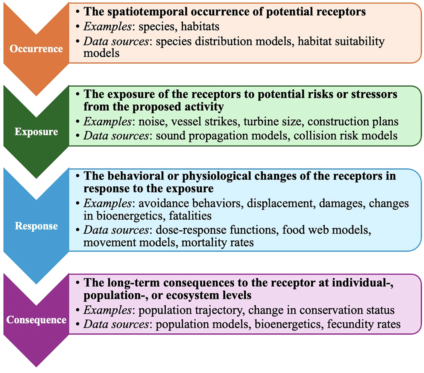
The elements of the “occurrence, exposure, response, consequence” risk assessment framework as described and used by the US Navy for their Integrated Comprehensive Monitoring Program for marine species, with examples and potential data sources. The figure is adapted from an unpublished presentation by Saana Isojunno, Centre for Research into Environmental and Ecological Modelling (CREEM), University of St. Andrews (Isojunno and Thomas, 2022).
Here we employ widely used spatial distribution models (SDMs) for 84 marine life taxa to evaluate their occurrence within wind energy lease areas (WELAs) and five subregions along the US Atlantic coast to identify spatiotemporal overlaps of marine life and offshore wind activities. This analysis aims to better understand the species, time periods, and areas that may be most vulnerable to potential OSW impacts, helping inform the prioritization of mitigation and monitoring efforts. For each of the 29 active Atlantic WELAs, we calculated the average monthly predicted densities for 13 marine mammal taxa (12 species and one guild), 49 seabird species, and four sea turtle species. We also calculated the average annual density for 18 additional marine mammal taxa (14 species and four guilds) for which only year-round average predictions were available. To provide a more focused and representative subset for this assessment and enable a clearer interpretation of risk across multiple taxa, we concentrated more closely on 11 focal species chosen to capture a range of spatiotemporal patterns, behaviors, conservation statuses, and ecologies. The focal species include four marine mammal, three avian, and four sea turtle species.
The marine mammal focal species are fin whales (Balaenoptera physalus), humpback whales (Megaptera novaengliae), minke whales (Balaenoptera acutorostrata), and North Atlantic right whales (Eubalaena glacialis). North Atlantic right whales, listed as “critically endangered” on the IUCN Red List (Cook, 2020), have been a primary focus of monitoring and mitigation in the region. While minke and humpback whales (Northwest Atlantic population) are currently listed as “least concern” (Cook, 2018a, 2018c), both species, as well as North Atlantic right whales, are currently experiencing an unusual mortality event in the region, as defined by the Marine Mammal Protection Act (MMPA 16 U.S.C. § 1421h(9)), highlighting the importance of continued study (Silber et al., 2023; Steinkamp, 2008; Congressional Research Service, 2024). Fin whales are listed as “vulnerable” and have limited migratory movement, making them more sensitive to displacement risk (Cook, 2018b; Davis et al., 2020).
The avian species selected—red-throated loons (Gavia stellata), northern gannets (Morus bassanus), and great black-backed gulls (Larus marinus)—were chosen due to their high sensitivity to collision and displacement and their habitat use patterns (Willmott et al., 2023; Heinänen et al., 2020; Peschko et al., 2021; Fauchald et al., 2024). While all three bird species are listed as “least concern” on the IUCN Red List (BirdLife International, 2018a, 2018c, 2018b), red-throated loons and northern gannets are both designated as “priority” under the Bird Conservation Region 30 (BCR30) from the North American Bird Conservation Initiative and as “high concern” by the Atlantic Marine Bird Conservation Cooperative (AMBCC) (Stepanuk et al., 2023; Marine Bird Species Priority List – July 2014, 2014; Curtice et al., 2019). Additionally, great black-backed gulls are year-long residents in the northeast, making them more vulnerable to potential habitat degradation (Welcker and Nehls, 2016; Goodale et al., 2019).
Although sea turtles are not often the focus of OSW studies, they may be particularly vulnerable due to their strong fidelity to migratory routes and critical habitats as well as their attraction to artificial light and structures, which could increase their overlap with WELAs (Secor et al., 2025). All four of the modeled sea turtle species—green (Chelonia mydas), Kemps ridley (Lepidochelys kempii), leatherback (Dermochelys coriacea), and loggerhead (Caretta caretta)—were considered focal species for this analysis and are all listed on the IUCN Red List. Greens, who are considered “endangered”, and Kemps ridleys, who are listed as “critically endangered”, are especially tied to specific nesting sites, raising concerns about displacement risk (Wibbels and Bevan, 2019; Seminoff, 2023; Secor et al., 2025), while leatherbacks and loggerheads, both classified as “vulnerable”, may be sensitive to the noise frequencies produced by OSW activities (Wallace et al., 2013; Bailey et al., 2014; Casale and Tucker, 2017).
To provide further context for this analysis, we use the subregional divisions—Gulf of Maine (GOM), Southern New England (SNE), New York/New Jersey Bight (NYNJB), Central US Atlantic (CA), and Southeastern US Atlantic (SEA)—established by the Regional Wildlife Science Collaborative (Figure 2). To account for regional variations in species distribution and to create a standardized context for comparability across the region, we calculated the 90th percentile of monthly density, hereafter referred to as “thresholds”, for each species across these divisions. This approach highlights locations and time periods of particularly high species occurrence, identifying potential areas of elevated risk and facilitating the prioritization of monitoring and mitigation.
Figure 2
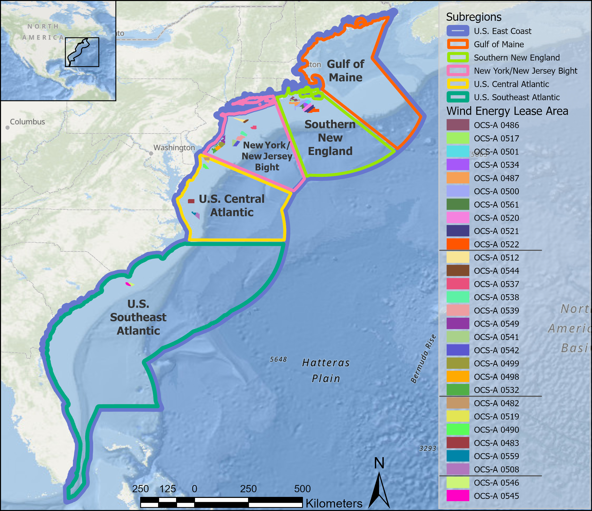
Map of the Atlantic coast of the US with the RWSC-defined subregions and active lease sites used in the analysis. In the legend, the WELAs are ordered by latitude from north to south, with black horizontal lines marking subregion boundaries: Southern New England (SNE), New York–New Jersey Bight (NYNJB), Central Atlantic (CA), and South Atlantic (SEA) in descending order.
As OSW development expands across the US OCS, understanding the cumulative and interconnected nature of its ecological effects—across regions, seasons, and life stages—will be critical. However, major knowledge gaps persist in predicting the long-term, population-level outcomes of these overlapping effects, particularly due to the complexity of ecological connectivity and impacts of concurrent stressors (Methratta et al., 2023; Silber et al., 2023). By establishing a robust baseline of species occurrence, this work provides a critical foundation to integrate wildlife distribution patterns into broader, multi-faceted risk frameworks. These insights are essential not only for informing near-term mitigation and monitoring efforts but also for supporting more proactive spatial planning that aligns OSW expansion with long-term conservation and sustainability goals.
2 Materials and methods
2.1 Data resources and spatial extent
2.1.1 Species distribution data
The species distribution products used in this study are density surface models (DSMs) that cover 84 marine taxa, including 31 marine mammal taxa (Table 1; Roberts et al., 2016, 2023), 49 seabird species (Table 2; Winship et al., 2023), and four sea turtle species (Table 3; DiMatteo et al., 2024). These publicly available DSMs were generated by relating quality-checked observation data from aerial or ship-based line-transect surveys to environmental variables using models to predict species density across spatial grid cells—marine mammals at a 5 km × 5 km resolution and a 10 km × 10 km resolution for seabirds and sea turtles. Each dataset included detailed metadata, such as platform type and characteristics (e.g., observation height, flight speed), and environmental conditions. This auxiliary information was used to develop detection probability functions that were incorporated into the models. All DSMs reflect composite predictions across their respective period of data collection (Table 4), averaged per calendar month, except 18 marine mammal taxa that were at a year-round temporal resolution. For more details about each of the datasets and access information, see Table 4.
Table 1
| Dataset | Description | Citation | Temporal extent | Temporal resolution | Spatial extent | Spatial resolution/unit |
|---|---|---|---|---|---|---|
| Wind energy lease area outlines | BOEM distributed outlines of all active WELAs with project names and other data attributes | BOEM, 2024 | Current listings as of 12/12/24 | — | — | — |
| Subregions | US Atlantic coast subregions defined by the RWSC | RWSC (Regional Wildlife Science Collaborative for Offshore Wind), 2024 | — | — | US Atlantic coast EEZ from Maine to southern tip of Florida | — |
| Marine mammals | Modeled absolute density surfaces for 31 marine mammal taxa | Roberts et al., 2016, 2023 | 1998–2020 | Monthly (13 taxa: 12 species and 1 guild) and year-round (18 taxa: 14 species and 4 guilds) | US Atlantic coast EEZ from Maine to the southern tip of Florida | 5 km × 5 km; animals per 100 km2 |
| Avians | Modeled relative density surfaces for 49 marine bird species | Winship et al., 2023 | 1998–2020 | Monthly | US and Canadian Atlantic EEZ from Nova Scotia to the southern tip of Florida | 10 km × 10 km; animals per strip transect segment |
| Sea turtles | Modeled absolute density surfaces for four sea turtle species | DiMatteo et al., 2024 | 2003–2019 (green turtle only 2010–2019) | Monthly | US Atlantic EEZ from the Gulf of Maine to the northern Florida Keys | 10 km × 10 km; animals per 1 km2 |
Summary of the five primary datasets used as spatial inputs throughout the spatial analysis workflow.
Table 2
| Common name | Scientific name/taxon | Taxonomic grouping | Time-step | IUNC status | ESA status |
|---|---|---|---|---|---|
| Atlantic spotted dolphin | Stenella frontalis | Species | Month | Data deficient | Not listed |
| Mesoplodont beaked whales | Mesoplodon spp. | Guild | Year-round | Varies by species | Varies by species |
| Blue whale | Balaenoptera musculus | Species | Year-round | Endangered | Endangered |
| Common bottlenose dolphin | Tursiops truncatus | Species | Month | Least concern | Not listed |
| Clymene dolphin | Stenella clymene | Species | Year-round | Data deficient | Not listed |
| Fin whale | Balaenoptera physalus | Species | Month | Vulnerable | Endangered |
| False killer whale | Pseudorca crassidens | Species | Year-round | Near threatened | Not listed |
| Frasers dolphin | Lagenodelphis hosei | Species | Year-round | Least concern | Not listed |
| Cuviers beaked whale | Ziphius cavirostris | Species | Year-round | Least concern | Not listed |
| Rissos dolphin | Grampus griseus | Species | Month | Least concern | Not listed |
| Harbor porpoise | Phocoena phocoena | Species | Month | Least concern | Not listed |
| Humpback whale | Megaptera novaeangliae | Species | Month | Least concern | Endangered |
| Killer whale | Orcinus orca | Species | Year-round | Data deficient | Not listed |
| Melon headed whale | Peponocephala electra | Species | Year-round | Least concern | Not listed |
| Common minke whale | Balaenoptera acutorostrata | Species | Month | Least concern | Not listed |
| North Atlantic right whale | Eubalaena glacialis | Species | Month | Critically endangered | Endangered |
| Northern bottlenose whale | Hyperoodon ampullatus | Species | Year-round | Data deficient | Not listed |
| Pilot whales | Globicephala spp. | Guild | Year-round | Varies by species | Varies by species |
| Pantropical spotted dolphin | Stenella attenuata | Species | Year-round | Least concern | Not listed |
| Pygmy killer whale | Feresa attenuata | Species | Year-round | Data deficient | Not listed |
| Rough-toothed dolphin | Steno bredanesis | Species | Year-round | Least concern | Not listed |
| Short-beaked common dolphin | Delphinus delphis | Species | Month | Least concern | Not listed |
| Sei whale | Balaenoptera borealis | Species | Month | Endangered | Endangered |
| Spinner dolphin | Stenella longirostris | Species | Year-round | Least concern | Not listed |
| Sperm whale | Physeter macrocephalus | Species | Month | Vulnerable | Endangered |
| Striped dolphin | Stenella frontalis | Species | Year-round | Least concern | Not listed |
| Unidentified beaked whales | Mesoplodon spp. | Guild | Year-round | Varies by species | Varies by species |
| Dwarf and pygmy sperm whales | Kogia spp. | Guild | Year-round | Data deficient | Not listed |
| Seals | Phocidae | Guild | Month | Varies by species | Varies by species |
| White beaked dolphin | Lagenorhynchus albirostris | Species | Year-round | Least concern | Not listed |
| Atlantic white-sided dolphin | Lagenorhynchus acutus | Species | Month | Least concern | Not listed |
List of marine mammal taxa used in the analysis with their taxonomic grouping and temporal resolution specified.
The four focal species are presented in bold.
Table 3
| Common name | Scientific name | AMBCC vulnerability listing | BCR listing | IUNC status | ESA status |
|---|---|---|---|---|---|
| Arctic tern | Sterna paradisaea | Medium concern | Not listed | Least concern | Not listed |
| Atlantic puffin | Fratercula arctica | High concern | Not listed | Vulnerable | Not listed |
| Audubons shearwater | Puffinus lherminieri | High concern | High priority | Least concern | Not listed |
| Band-rumped storm-petrel | Hydrobates castro | Medium concern | Not listed | Least concern | Endangered |
| Black guillemot | Cepphus grylle | Not listed | Not listed | Least concern | Not listed |
| Black scoter | Melanitta americana | Medium concern | High priority | Near threatened | Not listed |
| Black tern | Chlidonias niger | Medium concern | Not listed | Least concern | Not listed |
| Black-capped petrel | Pterodroma hasitata | High concern | Not listed | Endangered | Endangered |
| Black-legged kittiwake | Rissa tridactyla | Medium concern | Not listed | Vulnerable | Not listed |
| Bonapartes gull | Chroicocephalus philadelphia | Not listed | Not listed | Least concern | Not listed |
| Bridled tern | Onychoprion anaethetus | Low concern | High priority | Least concern | Not listed |
| Brown pelican | Pelecanus occidentalis | Medium concern | Not listed | Least concern | Not listed |
| Common eider | Somateria mollissima | High concern | High priority | Near threatened | Not listed |
| Common loon | Gavia immer | High concern | Not listed | Least concern | Not listed |
| Common murre | Uria aalge | High concern | Not listed | Least concern | Not listed |
| Common tern | Sterna hirundo | Not listed | Moderate priority | Least concern | Not listed |
| Corys shearwater | Calonectris borealis | Medium concern | Moderate priority | Least concern | Not listed |
| Double-crested cormorant | Phalacrocorax auritus | Not listed | Not listed | Least concern | Not listed |
| Dovekie | Alle | Not listed | Not listed | Least concern | Not listed |
| Forsters tern | Sterna forsteri | Not listed | High priority | Least concern | Not listed |
| Great black-backed gull | Larus marinus | Not listed | Not listed | Least concern | Not listed |
| Great shearwater | Ardenna gravis | Medium concern | High priority | Least concern | Not listed |
| Great skua | Stercorarius skua | Not listed | Not listed | Least concern | Not listed |
| Herring gull | Larus argentatus | Not listed | Not listed | Least concern | Not listed |
| Horned grebe | Podiceps auritus | Not listed | High priority | Vulnerable | Not listed |
| Laughing gull | Leucophaeus atricilla | Low concern | Not listed | Least concern | Not listed |
| Leachs storm-petrel | Oceanodroma leucorhoa | Medium concern | Not listed | Vulnerable | Not listed |
| Least tern | Sternula antillarum | High concern | High priority | Least concern | Not listed |
| Long-tailed duck | Clangula hyemalis | High concern | High priority | Vulnerable | Not listed |
| Manx shearwater | Puffinus | Medium concern | Moderate priority | Least concern | Not listed |
| Northern fulmar | Fulmarus glacialis | Not listed | Not listed | Least concern | Not listed |
| Northern gannet | Morus bassanus | High concern | High priority | Least concern | Not listed |
| Parasitic jaeger | Stercorarius parasiticus | Not listed | Not listed | Least concern | Not listed |
| Pomarine jaeger | Stercorarius pomarinus | Not listed | Not listed | Least concern | Not listed |
| Razorbill | Alca torda | High concern | Moderate priority | Least concern | Not listed |
| Red phalarope | Phalaropus fulicarius | Medium concern | Moderate priority | Least concern | Not listed |
| Red-breasted merganser | Mergus serrator | Not listed | Moderate priority | Least concern | Not listed |
| Red-necked phalarope | Phalaropus lobatus | High concern | Moderate priority | Least concern | Not listed |
| Red-throated loon | Gavia stellata | High concern | Highest priority | Least concern | Not listed |
| Ring-billed gull | Larus delawarensis | Not listed | Not listed | Least concern | Not listed |
| Roseate tern | Sterna dougallii | High concern | Highest priority | Least concern | Endangered |
| Royal tern | Thalasseus maximus | Medium concern | Moderate priority | Least concern | Not listed |
| Sooty shearwater | Ardenna grisea | Not listed | Not listed | Near threatened | Not listed |
| Sooty tern | Onychoprion fuscatus | Low concern | Not listed | Least concern | Not listed |
| South polar skua | Stercorarius maccormicki | Not listed | Not listed | Least concern | Not listed |
| Surf scoter | Melanitta perspicillata | Medium concern | High priority | Least concern | Not listed |
| Thick-billed murre | Uria lomvia | Not listed | Not listed | Least concern | Not listed |
| White-winged scoter | Melanitta deglandi | High concern | High priority | Least concern | Not listed |
| Wilsons storm-petrel | Oceanites oceanicus | Not listed | Not listed | Least concern | Not listed |
List of avian species used in this analysis with their respective AMBCC, BCR, IUCN, and ESA statuses.
The distribution data for these species have a 10 km × 10 km spatial resolution and a monthly temporal resolution. The three focal species are presented in bold.
Table 4
| Common name | Scientific name | IUCN status | ESA listing |
|---|---|---|---|
| Green sea turtle | Chelonia mydas | Endangered | Endangered |
| Kemps ridley sea turtle | Lepidochelys kempii | Critically endangered | Endangered |
| Leatherback sea turtle | Dermochelys coriacea | Vulnerable | Endangered |
| Loggerhead sea turtle | Caretta | Vulnerable | Endangered |
List of sea turtle species used in this analysis with their respective IUCN and ESA statuses.
The distribution data for these species have a 10 km × 10 km spatial resolution and a monthly temporal resolution. All of the four species listed are considered focal species in this analysis.
Density calculations were used instead of abundance to account for the varying sizes of WELAs and subregions, facilitating comparability between these areas. To maintain data integrity, each dataset was used at its maximum temporal and spatial resolution and retained in its original coordinate reference system. It is important to note that while the marine mammal and sea turtle models applied distance sampling techniques to estimate absolute density (individuals per unit area), the seabird models estimate relative density (an index of presence rather than of absolute abundance). This is because distance sampling is generally not feasible for seabird surveys due to missed detections and movement bias. To allow for comparison across avian species, we convert our calculations to proportional density (see Section 2.2 Analysis).
2.1.2 Spatial boundaries
The study area covers over 886,000 km2, comprising the US East Coast Exclusive Economic Zone (EEZ), extending from the shore out to approximately 200 nautical miles, from Maine to Florida. To subdivide this large area and provide ecological context for the calculations, we used delineations provided by the RWSC that were based on ecological, political, and geographic characteristics, yielding five subregions: Gulf of Maine, Southern New England, New York/New Jersey Bight, Central US Atlantic, and Southeastern US Atlantic as shown in Figure 2.
To delineate the WELAs, we use publicly available polygon shapefiles distributed by the Bureau of Ocean Energy Management (BOEM) (last update 12/12/24). Three provisional sites, Block Island, CVOW, and the GOM Research Lease, were removed from the analyses because of their operational status and significantly smaller extents, yielding a total of 29 WELAs that were analyzed. A 10-km geodesic buffer was applied to each WELA to account for the movement of marine species and potential leakage of noise and other OSW effects beyond lease boundaries. This buffer aligns with initial estimations of construction sound propagation distances for the hearing frequency ranges of baleen whales and sea turtles (Piniak, 2012; Best and Halpin, 2019; Amaral et al., 2020), the commonly accepted minimum acoustic detection range for baleen whales (Van Parijs et al., 2021), and seabird displacement studies (Garthe et al., 2023). Exploratory assessments showed that the density estimates with and without the buffer were similar; however, the 10-km buffer ensured that potential interaction risks were accounted for in a manner consistent with existing research, offering a conservative yet reasonable estimate of species occurrence.
2.2 Analysis
For each month and all 84 taxa, we analyzed species occurrence within WELAs by extracting the predicted density values for all grid cells that fell within the buffered boundaries of each WELA. We then computed the spatial average of these values to generate a monthly (or yearly) mean density per species per WELA. These averages were used to identify seasonal patterns and compare with subregional thresholds.
To evaluate whether certain WELAs had months with consistently high species density, we established a threshold for comparison between the WELAs and their respective subregions: Gulf of Maine, Southern New England, New York/New Jersey Bight, US Central Atlantic, and US Southeast Atlantic. We selected the 90th percentile of the subregions monthly (or yearly) densities as the threshold, following established methods from previous studies assessing marine life risk [marine mammals (Avila et al., 2018; Rockwood et al., 2021), sea birds (Studwell et al., 2021), and sea turtles (Abecassis et al., 2013)] and discussions with stakeholders. These values were computed independently for each calendar month (or yearly average) and used as comparative benchmarks to identify whether each WELA had above-threshold densities in any given time period and consider regional ecological patterns. These values were visualized as various heatmaps and analyzed to identify patterns and potential areas of concern that could inform OSW management. Although the Gulf of Maine subregion was included in these analyses, it contains no active WELAs, so its values are not referenced further in this paper.
To account for the relative density values from the seabird DSMs and facilitate accurate species comparisons, we standardized the predicted relative density values using a normalizing factor before calculating the average monthly densities for each WELA and each subregions 90th percentile threshold. This method, adapted from Winship et al. (2023), scales the predicted relative density by dividing each grid cell of the DSM by the mean density across all grid cells for each species and month prior to calculating the monthly WELA averages and subregional thresholds. This results in a scale where values above 1 indicate areas of above-average density, while values below 1 indicate areas of below-average density. Normalizing in this way highlights spatial patterns and areas of particularly high or low relative density, without distorting interspecies comparisons. However, it is important to note that these values are still not equivalent to absolute density and cannot be directly interpreted as individual counts. Furthermore, because the DSMs of the other taxa in this study are still presented as absolute values, this approach does not facilitate cross-taxa comparisons.
While the calculations were completed for all 84 marine taxa, we selected 11 species to act as focal species. These were chosen to represent a variety of temporal, spatial, and ecological properties and were also informed by regional management relevance and stakeholder input. The focal species include four marine mammals (fin whales, humpback whales, minke whales, and North Atlantic right whales), three avian species (red-throated loons, northern gannets, and great black-backed gulls), and all four modeled sea turtle species (green, Kemps ridley, leatherback, and loggerhead).
3 Results
This study calculated the predicted densities of 84 marine taxa across 29 WELAs in the US Atlantic region. For all taxa, the average monthly (or annual, for the 18 year-round marine mammal taxa) density statistics for each WELA, 90th percentile thresholds for all subregions, differences between the densities and thresholds, and summary tables of species with the highest overall densities and densities above the 90th percentile in WELAs can be found in the Supplementary Material.
3.1 Marine mammals
All of the 13 monthly marine mammal taxa were predicted to have some level of presence across the lease areas; however, the two southernmost lease areas, OCS-A 0546 and OCS-A 0545, showed no presence for several species (Rissos dolphin, minke whale, white-sided dolphins, and sei whale) in any month. Additionally, three taxa (harbor porpoises, North Atlantic right whales, and seals) showed no predicted presence in two of the CA WELAs, OCS-A 0508 and OSC- A 0559, during selected months. Of the 18 year-round marine mammal taxa, seven were not present in any of the WELAs (false killer whale, Frasers dolphin, melon headed dolphin, northern bottlenose whale, pygmy killer whale, spinner dolphin, and white beaked dolphin), and two—blue whale and killer whale—had no presence in the two southern leases.
The highest overall densities were short-beaked common dolphin in SNE and NYNJB (n = 40.0 in September in OCS-A 0522 and n = 48.2 in October in OCS-A 0537), bottlenose dolphin in CA (n = 27.9 in August in OCS-A 0490), and Atlantic spotted dolphin in SEA (n = 21.4 in July in OCS-A 0545). The species with the highest difference between density and the subregional 90th percentile threshold (hereafter: Δ) for each subregion were seals in SNE (Δ = 6.50 in April in OCS-A 0501), bottlenose dolphin in NYNJB (Δ = 13.3 in August in OCS-A 0532), and Atlantic white-sided dolphin in CA and SEA (Δ = 14.6 in July in OCS-A 0508 and Δ = 9.48 in July in OCS-A 0545).
Among the four focal species specifically, we can identify patterns of seasonal and spatial density (Figure 3). Fin whales exhibited seasonal density peaks from May through September, with minor peaks in December and January, particularly in SNE. However, these densities never exceeded the subregional threshold. In the NYNJB, some WELAs had persistent presence from December to November, but only one lease, OCS-A 0537, surpassed the threshold in a single month (July), and in the CA, OCS-A 0508 exceeded the threshold in March.
Figure 3
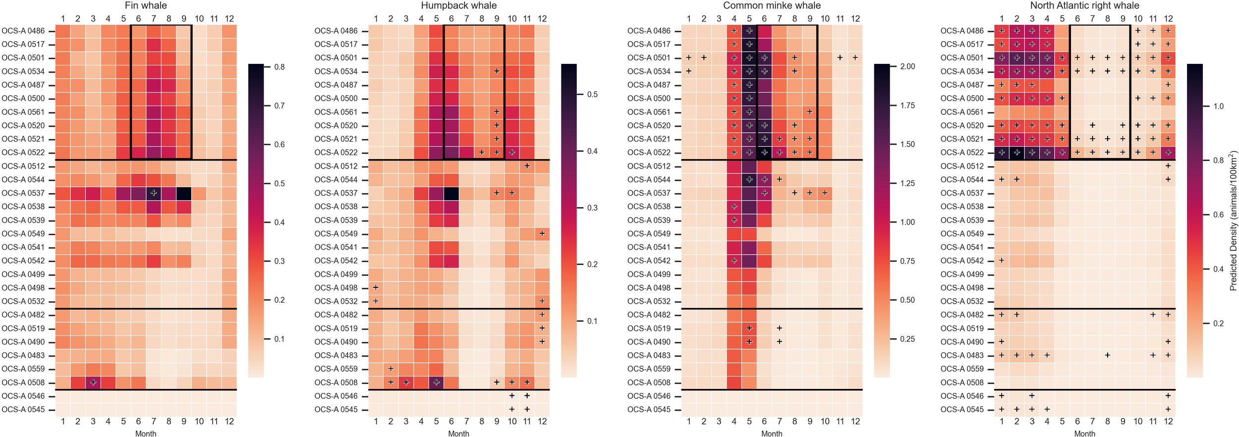
Heatmaps depicting mean monthly densities (animals/100 km²) for each focal marine mammal species—fin, humpback, minke, and North Atlantic right whale—within each wind energy lease area (WELA). WELAs are ordered by latitude, from north to south, with black horizontal lines marking subregion boundaries: Southern New England (SNE), New York–New Jersey Bight (NYNJB), Central Atlantic (CA), and South Atlantic (SEA) in descending order. Cells marked with a plus sign indicate densities above the 90th percentile for the corresponding subregion. The black boxes outline the months discussed in the discussion with notable differences in species occurrence among the focal species. Note: The color bar is not normalized between species.
Humpback whales demonstrated the lowest densities overall, with their highest density observed in OCS-A 0537 in June. They displayed two distinct peaks: April through June and October through November. Four SNE leases (OCS-A 5061, 5020, 5021, and 5022) exceeded the threshold in September, with some sites exceeding it in August and October as well. The largest difference over the threshold for humpbacks occurred in OCS-A 0508 in May (Δ = 0.163), with additional months exceeding the threshold in February, March, September, October, and November.
Minke whales had a pronounced peak in all subregions besides SEA, with the highest densities occurring April through May. In SNE, all 10 leases surpassed the threshold during these months, with OCS-A 0501 exceeding it for 8 months out of the year, though not consecutively. Persistent elevated densities from April to September were observed in two leases in SNE, OCS-A 0521 and 0522. The largest difference was in May in OCS-A 0501 (Δ = 0.418).
North Atlantic right whales exhibited a seasonal peak in SNE from December to May. Four of the SNE leases (OCS-A 0501, 0534, 0521, and 0522) had densities exceeding the thresholds for the entire year, with only OCS-A 0561 falling below the threshold in all months. The seasonal peak in SNE was mirrored throughout the coast, with OCS-A 0483 and OCS-A 0545 exceeding the thresholds for 7 and 5 months, respectively.
Although we cannot analyze the temporal patterns of the 18 taxa with only year-round distributions, we can identify spatial patterns (Figure 4). Of these 18 taxa, pilot whales had the highest densities in all lease areas besides the two SEA lease sites, where pantropical spotted dolphins and rough-toothed dolphins had the highest densities. OCS-A 0559 and OCS-A 0508, the two leases off the Outer Banks in North Carolina, had the most taxa with detectable average annual densities (greater than 0.02), including Clymene dolphins, pilot whales, pantropical spotted dolphins, and striped dolphins. None of the lease sites had densities exceeding the regional thresholds for any of the year-round taxa.
Figure 4
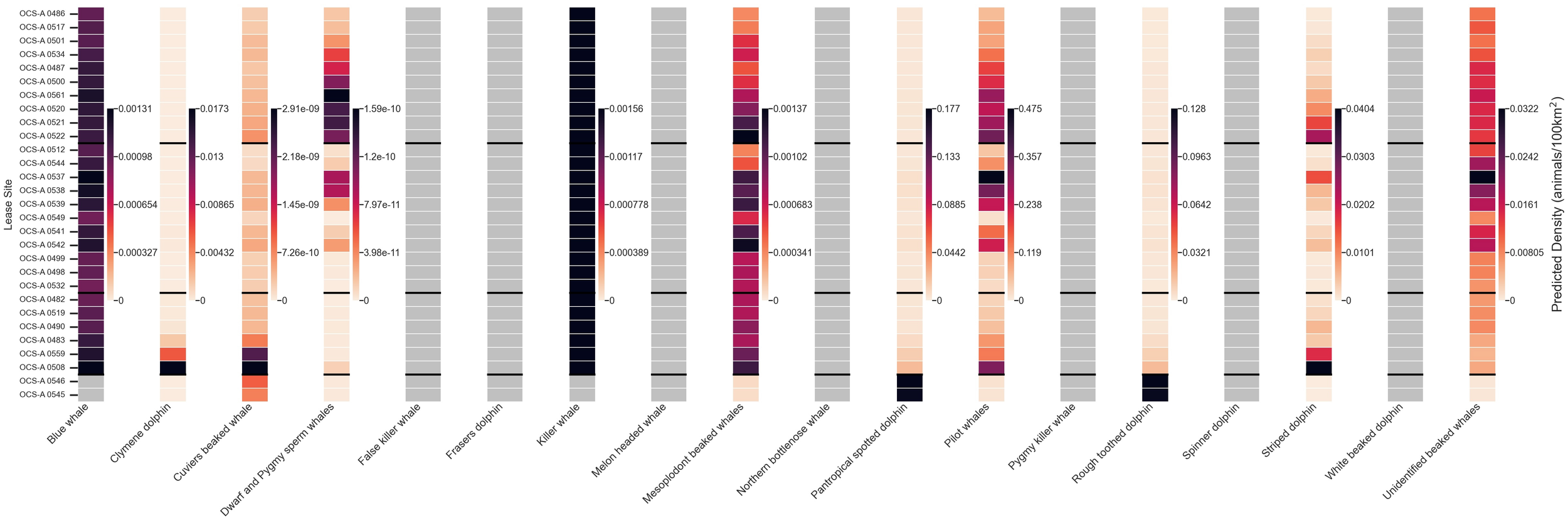
Heatmap depicting mean monthly densities (animals/100 km²) for all 18 year-round modeled marine mammal taxa within each wind energy lease area (WELA). WELAs are ordered by latitude, from north to south, with black horizontal lines marking subregion boundaries: Southern New England (SNE), New York–New Jersey Bight (NYNJB), Central Atlantic (CA), and South Atlantic (SEA) in descending order. No density values exceed the 90th percentile thresholds within any subregion. The gray cells represent areas with no predicted presence. Note: The color bar is not normalized between species.
3.2 Avian
All 49 species were predicted to be present in all 29 lease areas throughout the year. The species with the highest relative densities and relative densities above the 90th percentile in WELAs for each subregion are shown in Appendix C. The species with the highest relative densities were white-winged scoter in SNE, NYNJB, and CA (n = 20.1 in March in OCS-A 0486, n = 17.0 in January in OCS-A 0532, and n = 14.7 in February in OCS-A 0482, respectively) and red phalarope in SEA (n = 25.5 in January in OCS-A 0545).
The species with the highest difference between density and the 90th percentile threshold for each subregion was common eider in SNE (Δ = 13.6 in March in OCS-A 0486), white-winged scoter in NYNJB and CA (Δ = 8.96 in December in OCS-A 0532 and Δ = 11.8 in February in OCS-A 0482, respectively), black-legged kittiwake in SNE, NYNJB, and CA (Δ = 0.182 in December in OCS-A 0534, Δ = 0.0460 in January in OCS-A 0544, and Δ = 0.0605 in January in OCS-A 0519, respectively), and red phalarope in SEA (Δ = 18.1 in January in OCS-A 0545).
Among the focal species, northern gannets and red-throated loons exhibit clear seasonal patterns, while great black-backed gulls maintain a consistent presence year-round across all regions, except for SEA (Figure 5). Northern gannet density peaks shift across the coast over the course of the year. In SNE, higher relative densities are observed from April to November, especially in June, where the difference between density and subregional threshold is greatest in OCS-A 0486 (Δ = 2.99). This area also exceeds the threshold in all months except March. In NYNJB, peak relative densities occur from March to June and October to December. In CA, peaks are observed from February to April and November to December, while in SEA, the highest densities are found from November through March. In NYNJB, months with densities exceeding the threshold are more dispersed, while in CA and SEA, these months occur in succession—for instance, OCS-A 0546 in SEA maintains densities above the threshold for eight consecutive months, from October through May.
Figure 5
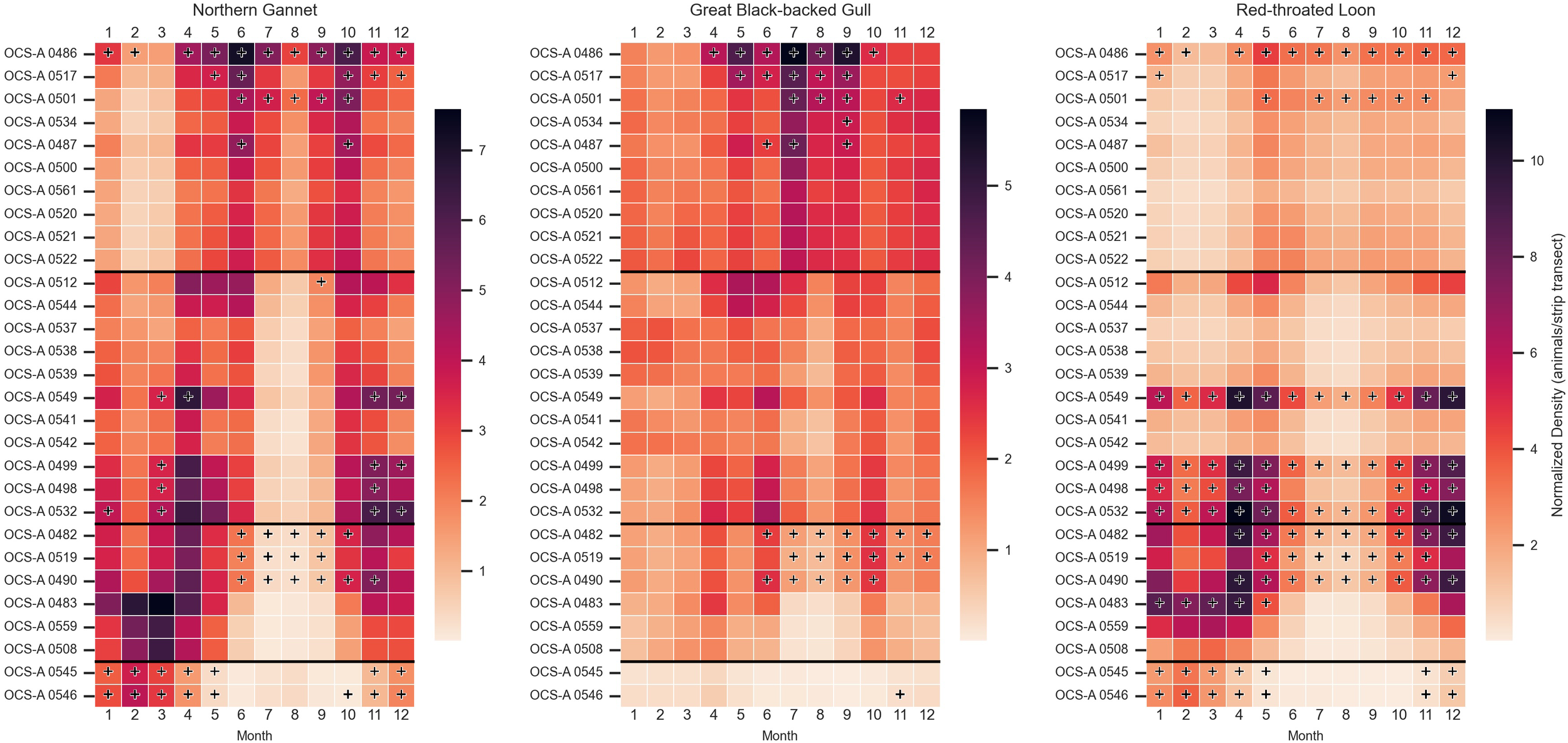
Heatmaps depicting normalized monthly densities (animals/ship transects) for each focal avian species—great black-backed gull, northern gannet, and red-throated loon—within each wind energy lease area (WELA). WELAs are ordered by latitude, from north to south, with black horizontal lines marking subregion boundaries: Southern New England (SNE), New York–New Jersey Bight (NYNJB), Central Atlantic (CA), and South Atlantic (SEA) in descending order. Cells marked with a plus sign indicate densities above the 90th percentile for the corresponding subregion. Note: The color bar is not normalized between species.
Red-throated loons exhibited lower overall relative densities in SNE but showed a slight peak from May to June and September–November. Two WELAs had densities exceeding the threshold for six or more months, with OCS-A 0486 exceeding the threshold in all months except March. Throughout the rest of the coast, peak densities were more pronounced, occurring from October to May in NYNJB, November to May in CA, and December to March in SNE. A clear spatial peak was observed in the WELAs further south in NYNJB and further north in CA. Seven lease sites in these areas had densities exceeding the threshold for seven or more months, including three in NYNJB (OCS-A 0549, 0499, and 0532), which exceeded the threshold year-round. OCS-A 0532 also had the highest density-threshold difference in December (Δ = 5.02). The two leases in SEA also had 7 months over the threshold.
While the presence of great black-backed gulls was more constant, there were higher densities in April through October. In SNE, OCS-A 0486 had higher than threshold numbers in 7 months, with the highest difference in September (Δ = 2.55). OCS-A 0482 in CA also had 7 months with higher than threshold numbers. There were no leases over the threshold in NYNJB and none in January through March across the whole coast.
3.3 Sea turtles
Sea turtles were predicted to occur in all WELAs throughout the year, though notable temporal gaps were observed in the densities of Kemps ridley and green sea turtles (Figure 6). These species had no predicted density for at least three consecutive months in 27 of the 29 lease sites. In contrast, the two SEA leases, OCS-A 0546 and OCS-A 0545, showed the year-round presence of all four sea turtle species. The overall densities for each WELA and densities above the 90th percentile threshold for each subregion are shown in Appendix C. All species exhibited a seasonal density peak from June through October, although the regional extent and duration of this peak varied by species.
Figure 6
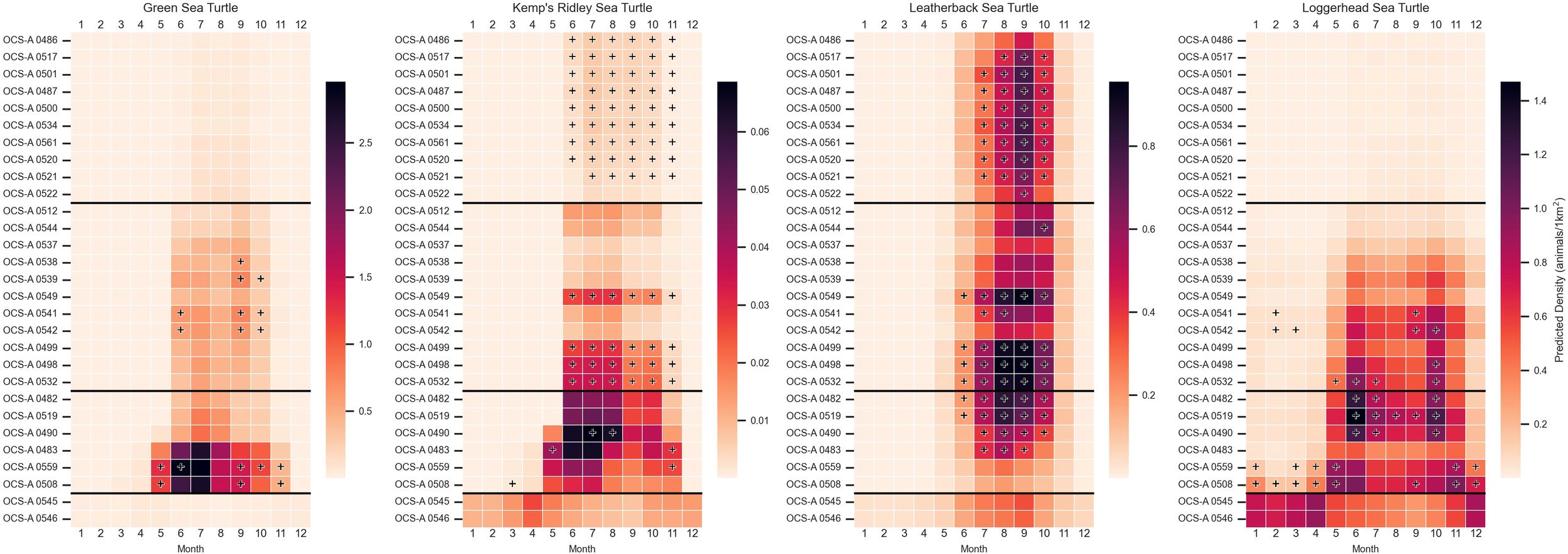
Heatmaps depicting mean monthly densities (animals/1 km²) for each modeled sea turtle species—green, Kemps ridley, leatherback, and loggerhead—within each wind energy lease area (WELA). WELAs are ordered by latitude, from north to south, with black horizontal lines marking subregion boundaries: Southern New England (SNE), New York–New Jersey Bight (NYNJB), Central Atlantic (CA), and South Atlantic (SEA) in descending order. Cells marked with a plus sign indicate densities above the 90th percentile for the corresponding subregion. The color bar is not normalized between species.
The species with the highest overall densities were leatherback for SNE (n = 0.777 in September in OCS-A 0501), loggerhead in NYNJB and SEA (n = 0.959 in June in OCS-A 0532 and n = 0.933 in April in OCS-A 0545), and green in CA (n = 2.96 in July in OCS-A 0559). The species with the highest difference between density and the 90th percentile threshold for each subregion was leatherback for SNE and NYNJB (n = 0.260 in September in OCS-A 0501 and n = 0.343 in August in OCS-A 0498) and loggerhead in CA (n = 0.428 in June in OCS-A 0519). No species exceeded the subregional threshold in any of the SEA WELAs.
Green sea turtles peaked from June through September in the NYNB and from May through November in parts of the CA. In the CA, densities exceeded the threshold for six consecutive months in OCS-A 0482, with the highest difference for the species occurring there in July (Δ = 2.65). In OCS-A 0559, densities were above the threshold for five non-consecutive months. Several other leases in CA exceeded thresholds as well, particularly in June, September, and October.
Leatherback turtles exhibited the strongest and most widespread peak, with elevated densities from June through October across the coast. There were 15 leases in SNE, NYNJB, and CA that had three or more months exceeding thresholds, all occurring between July through October. The highest difference in density for leatherbacks occurred in OCS-A 0482 in CA in September (Δ = 0.370).
Kemps ridley showed a similar pattern, though their presence was less pronounced in SNE and SEA, where densities appeared more consistent year-round. In SNE, 10 of the 11 SNE leases, excluding OCS-A 0522, exceeded thresholds from June through October. In the NYNJB, four leases followed a similar pattern, including OCS-A 0532, which recorded the highest difference in June (Δ= 0.0178).
Loggerheads had an extended peak from May through November, primarily in NYNJB and CA. While densities in SNE were lower and did not exceed any thresholds, the SEA showed year-round presence, with higher densities during the opposite months of NYNJB and CA, from November to April. In CA, all but one lease had at least 1 month over the threshold, with OCS-A 0508 showing 8 months and OCS-A 0559 showing 6 months above the threshold. Additionally, six leases in CA and NYNJB exceeded thresholds in October. The highest difference in density from the threshold occurred in OCS-A 0508 in CA in December (Δ = 0.365).
4 Discussion
This study represents the first application of current density surface models (DSMs) to assess the potential risks of OSW development to marine mammal, seabird, and sea turtle species along the US Atlantic coast. The results emphasize the substantial spatiotemporal variability in species distributions shaped by the complex migratory, behavioral, and habitat use patterns of these taxa (Best and Halpin, 2019; Silber et al., 2023; DiMatteo et al., 2024; Secor et al., 2025). By employing the OERC framework, we can tease apart these multifaceted ecosystem interactions by isolating individual risk components to provide the solid foundation needed for effective minimization and mitigation strategies. Although the focus of this assessment is on species occurrence, the initial phase of the OERC risk framework, the findings also offer insights into broader dimensions of species risk, such as potential conflicts, information gaps, and priorities for future research in OSW planning and mitigation.
As anticipated, the species assessed exhibit distinct seasonal distribution patterns tied to migration, foraging, breeding, and calving habitat preferences (Bailey et al., 2014; Best and Halpin, 2019; Silber et al., 2023; Morant et al., 2025; Secor et al., 2025)—for example, many avian species, including two of the focal species, northern gannet and red-throated loon, showed higher relative densities during the colder months in the more southern leases, while sea turtles peaked during the late summer and fall. Among the four focal baleen whale species, the three highly migratory species—humpback, minke, and North Atlantic right whales—showed more breaches of the 90th percentile density threshold than fin whales, who have been documented to have limited migratory movements and maintain a wide distribution year-round (Figure 3) (Risch et al., 2014; Davis et al., 2020; Silber et al., 2023; Secor et al., 2025). Similarly, the consistent presence of Kemps ridleys and loggerheads in the SEA subregion and the minimal seasonal variation in great black-backed gulls suggest that tailored management strategies may be necessary for species that remain near or within WELAs throughout the year. Although great black-backed gulls are not ESA-listed, they are of growing conservation concern due to their population decline, large size, and breeding activities in the GOM and SNE regions, making them more vulnerable to OSW collision and displacement risks (Willmott et al., 2023; Curtice et al., 2019; Goodale et al., 2019).
A further comparison of species density on a monthly time-step reveals critical differences in species occupancy that have direct implications on OSW mitigation strategies—for example, North Atlantic right whales were least abundant in SNE during the mid-late summer months, while minke, fin, and humpback whales exhibited high densities in that region at this time (demarcated by the black box in Figure 3). Such patterns have already informed management practices, such as limiting pile-driving activities to the summer and seasonal vessel speed restrictions to reduce risk to the critically endangered North Atlantic right whale (Silber et al., 2023; Stepanuk et al., 2023). However, these temporal differences in migratory patterns have been further complicated in recent years by the effects of climate change and prey field fluctuations, highlighting the need for regular monitoring, continuous investigation, and adaptive management approaches (Gulland et al., 2022; Lettrich et al., 2023; Silber et al., 2023; Secor et al., 2025).
A critical spatial variable to consider is the distance to the shore of the WELA. Many of the avian species showed higher densities in the lease sites within 50 km of the shore (Figure 7), such as OCS-A 0486 which exceeded the regional density threshold for all three focal avian species in at least 7 months (see Figure 5). This pattern is also evident for red-throated loons in NYNJB and CA, where all eight lease sites with elevated densities and threshold exceedances were within 50 km of the shore. In contrast, several of the year-round marine mammals showed higher densities in the leases further offshore, such as pilot whales, striped dolphins, mesoplodont beaked whales, and unidentified beaked whales (Figure 8). The offshore distributions of these more elusive and distant marine mammal species will play an increasingly important role as floating wind farms become more prevalent and OSW activities take up further offshore habitats. This wide variety of distributional patterns underscores the need for site-specific species data to inform effective mitigation planning.
Figure 7
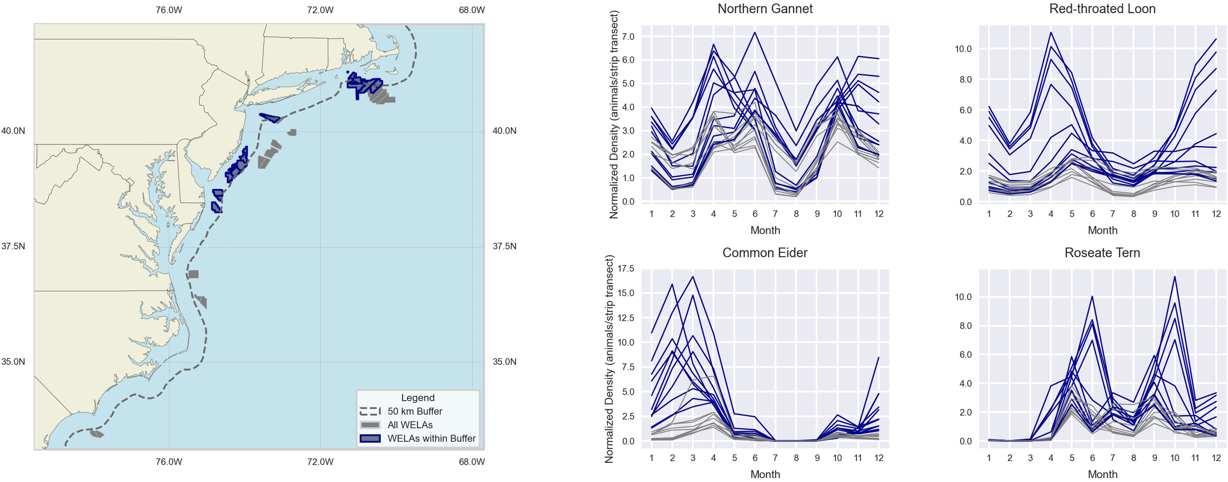
Time series showing the densities of two focal avian species and two other species. The blue lines illustrate density values in WELAs less than 50 km from the shore, and the gray lines illustrate density values in WELAs greater than 50 km from the shore. The Y-axis is not standardized.
Figure 8
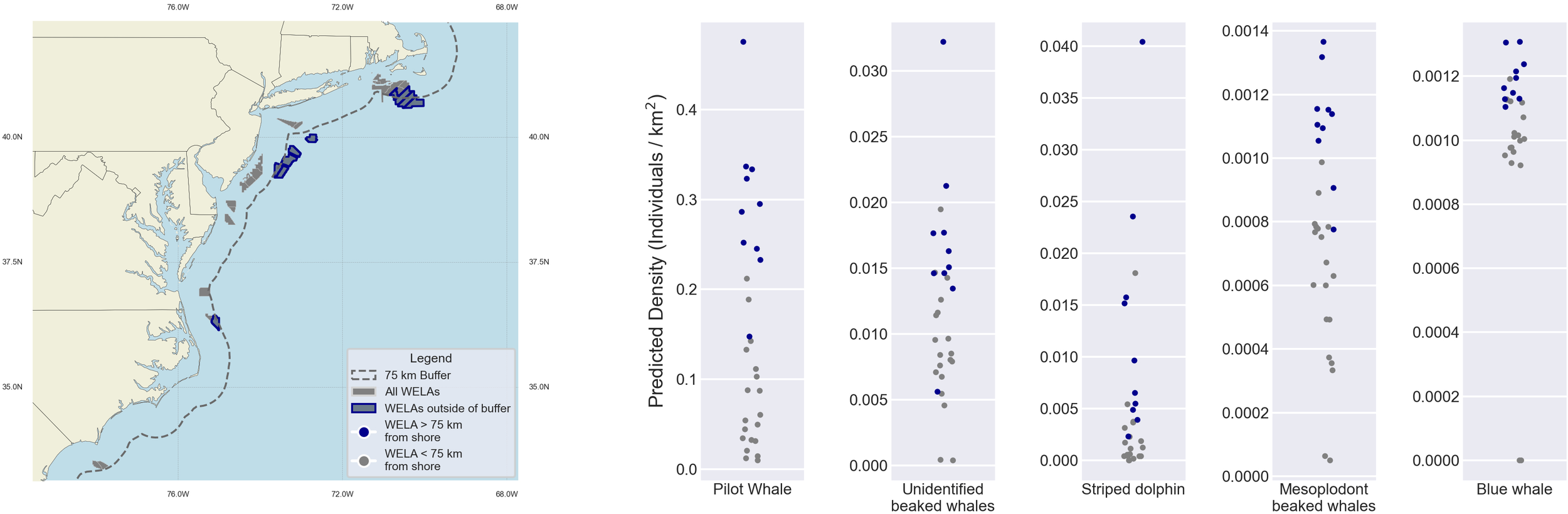
Strip plot showing the densities of four marine mammal taxa. The blue points illustrate density values in WELAs greater than 75 km from the shore, and the gray points illustrate density values in WELAs less than 75 km from the shore. The Y-axis is not standardized.
In addition to highlighting species of high concern, these results are also valuable to identify other species at risk from OSW development that have not been as consistently studied in that context. Green sea turtles were highly concentrated in the three lease sites around the Virginia–North Carolina border (OCS-A 0483, 0559, and 0508), emphasizing the need for more focused research on their habitat use in that area prior to OSW construction. Among marine mammals, harbor porpoises, bottlenose dolphins, and seals had the highest densities and persistently exceeded density thresholds, suggesting a heightened risk of disturbance (Figure 9). For seabirds, species such as the Bonapartes gull, common eider, common loon, laughing gull, surf scoter, and white-winged scoter were found to have densities higher than subregional thresholds throughout the subregions (Figure 10). Besides Bonapartes gull, these species are considered priority species under BCR30 and/or AMBCC with high sensitivity to collision and displacement, making them potentially at a greater risk from OSW activities (Steinkamp, 2008; Marine Bird Species Priority List – July 2014, 2014; Curtice et al., 2019; Goodale et al., 2019). While there is existing literature on the potential risk of OSW to many of these species—green sea turtles (Secor et al., 2025), harbor porpoises (Benhemma-Le Gall et al., 2021), bottlenose dolphins (Branstetter et al., 2018), seals (Best and Halpin, 2019), white-winged scoter, laughing gull, common loon, surf scoter (Best and Halpin, 2019; Goodale et al., 2019), and common eider (Beuth et al., 2017; Best and Halpin, 2019; Tanskanen et al., 2022)—these findings further highlight the importance of considering a broad range of species for OSW planning and mitigation efforts.
Figure 9
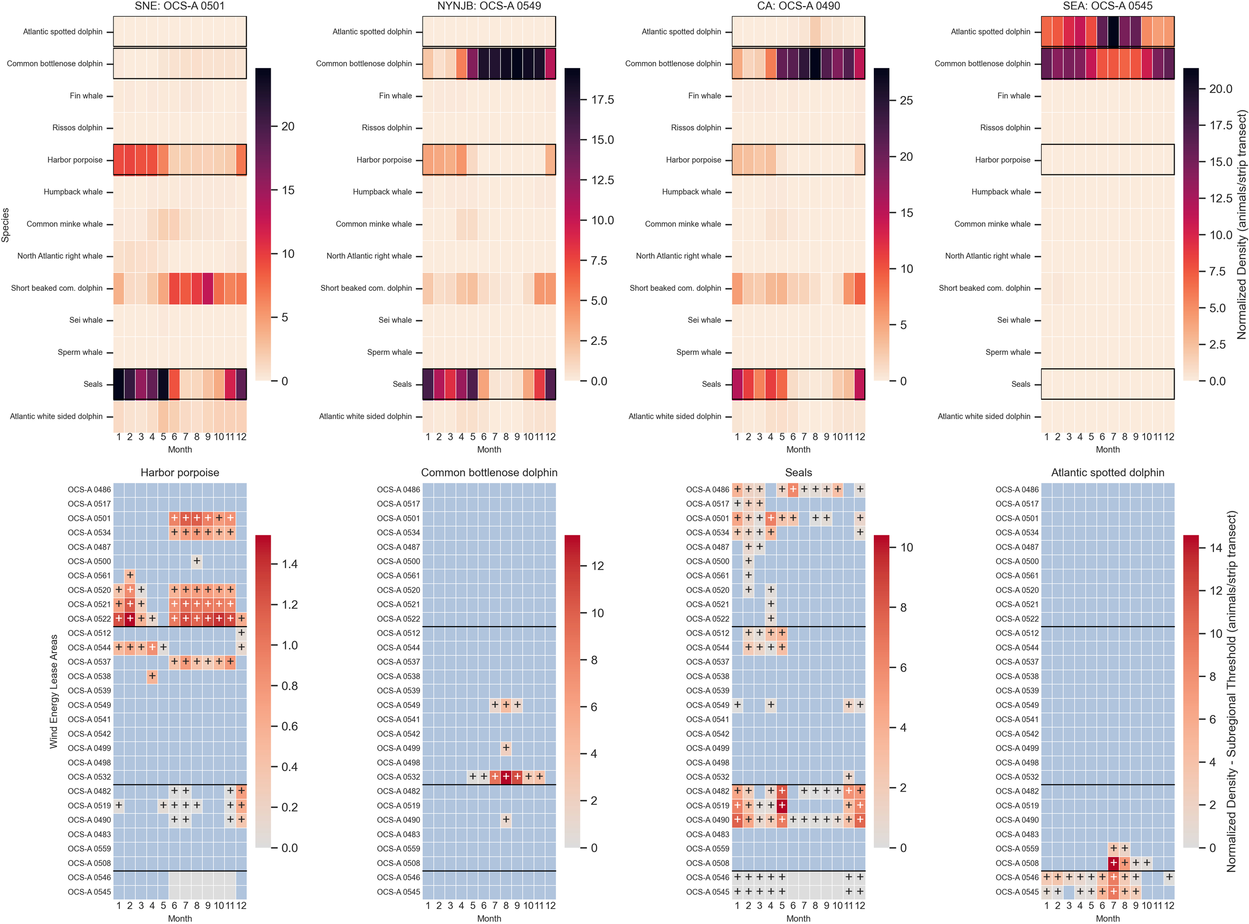
Heatmaps of the densities of the 13 monthly marine mammal taxa in five lease sites, one within each subregion, and the differences between density and subregional thresholds for four of the more abundant species. The color scale in the lower panels represents density difference: the blue cells indicate a species density below the subregional threshold, the solid gray cells denote no difference (typically due to the species absence in that WELA or month), and cells with a plus sign indicate a species density exceeding the threshold. The gray-to-red scale illustrates the magnitude of the exceedance, with deeper red indicating a greater difference above the threshold. The color bar is not normalized between species.
Figure 10
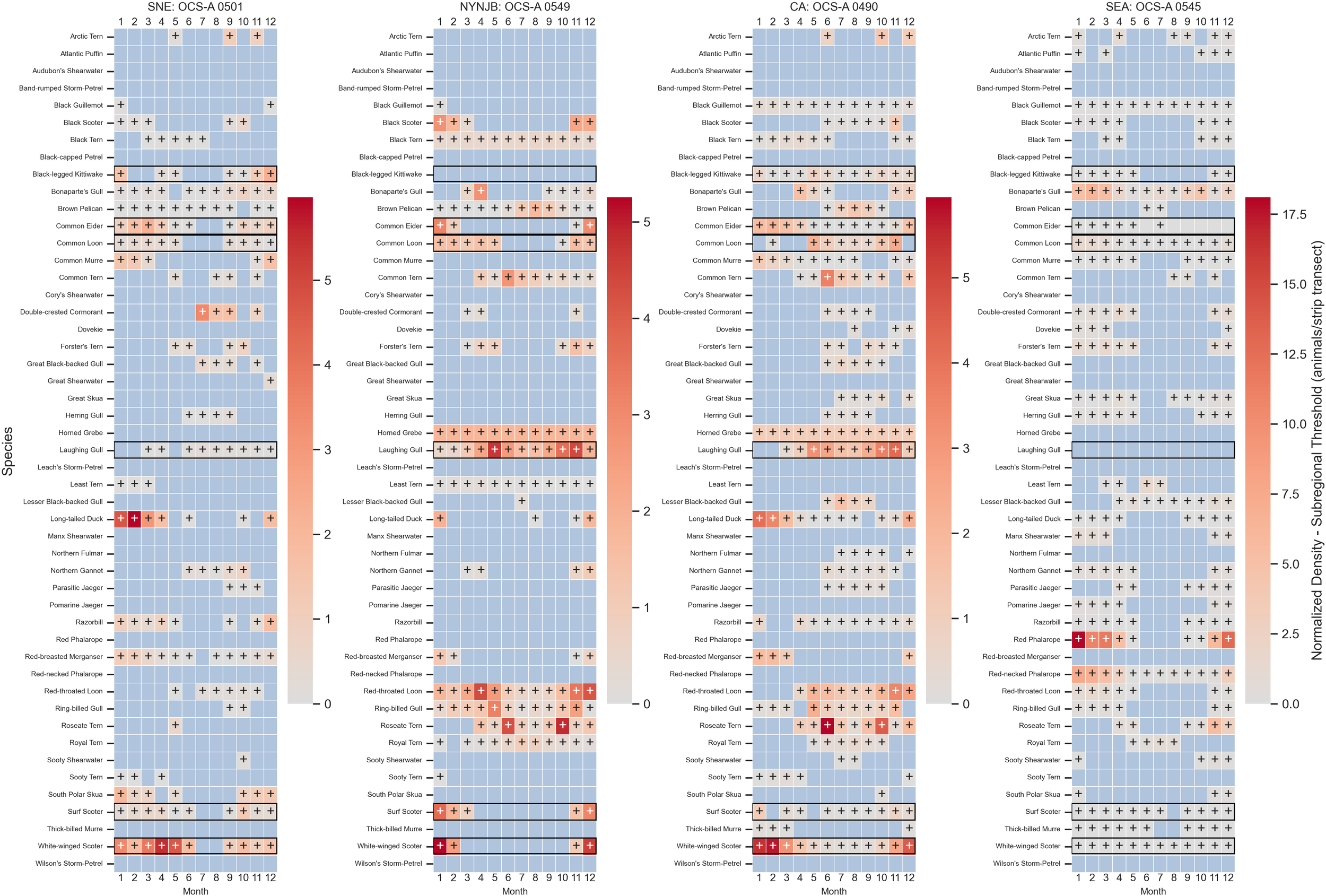
Heatmap of the difference in density to regional thresholds for all avian species in a lease area from each subregion. The most central leases were selected for each subregion to provide a characteristic view of the subregion as a whole; however, densities differ greatly within subregions. The color scale represents density difference: the blue cells indicate a species density below the subregional threshold, the solid gray cells denote no difference (typically due to the species absence in that WELA or month), and cells with a plus sign indicate a species density exceeding the threshold. The gray-to-red scale illustrates the magnitude of the exceedance, with deeper red indicating a greater difference above the threshold. The black rectangles highlight species with a higher persistence of months over the 90th percentile threshold.
Because this study was based on predictions from DSMs built using dynamic environmental covariates, it is essential to acknowledge the limitations associated with studying a highly dynamic and elusive marine ecosystem. The DSMs rely on visual observations, which are inherently subject to uncertainty from variable survey effort and detectability (Curtice et al., 2019; Sparks and DiMatteo, 2023; Roberts et al., 2023; Winship et al., 2023)—for example, low baleen whale densities predicted in the SEA during winter, despite known southern migrations for many species, may reflect limited survey coverage rather than a true absence (Roberts et al., 2023). Interannual variability in migration patterns, exacerbated by climate change, further challenges predictive modeling and underscores the need for ongoing monitoring (Sparks and DiMatteo, 2023; Roberts et al., 2023; Silber et al., 2023; Winship et al., 2023; Secor et al., 2025). These challenges are compounded for data-deficient species, many of which lack IUCN status or basic ecological information, making it difficult to fully assess risk. Addressing these limitations is essential to not only validate and improve model accuracy but to support more proactive and site-specific mitigation strategies. Doing so will require continued baseline studies, the integration of additional data streams (e.g., passive acoustic monitoring, telemetry), and investment in technological advancements (Macrander et al., 2022; Silber et al., 2023; Morant et al., 2025).
5 Conclusion
This foundational assessment provides the first large-scale, species-level assessment of predicted occurrence across all current WELAs throughout the US Atlantic Outer Continental Shelf. We identify both where and when species are most likely to overlap with OSW activities to establish a crucial ecological baseline to inform future OSW decision-making. As potential impacts are not uniform but shaped by species-specific traits, behaviors, movements, and vulnerabilities, conservation solutions cannot be one-size-fits-all, underscoring the need for nuanced, spatiotemporally informed mitigation strategies tailored to ecological context. The patterns presented in our findings, such as sustained high densities in specific lease areas or frequent exceedances of subregional thresholds, offer actionable data-driven guidance to align OSW development with conservation priorities. Our results show that each of the selected focal species exhibits levels of expected occurrence in WELAs that exceed the corresponding 90th percentile subregional density threshold at some point throughout the duration of the year. This finding suggests that all focal species are likely to experience exposure to OSW infrastructure in the US Atlantic in one or more instances each year.
As the initial phase in the OERC risk framework, these results lay the groundwork for incorporating species exposures, behavioral responses, and consequences that, when integrated, will offer a more comprehensive understanding of risk across taxa and geographies. Beyond its applications to OSW planning, the OERC risk framework and approach presented here provide broader utility for spatial planning, environmental impact assessments, evaluating the effectiveness of current mitigation strategies, and ecosystem-based management for sustainable development across multiple sectors and other environments.
While OSW development holds significant promise to advance renewable energy capacity, it must proceed with robust, science-based assessments such as this and be complemented by long-term monitoring throughout all phases of development to strengthen future models, inform management, and minimize unintended impacts to marine species and ecosystems. Although these results are only predictive, large-scale, ecosystem-wide studies remain essential to balance renewable energy development with the lasting conservation of marine habitats. By enhancing the knowledge base around OSW–wildlife interactions, we can better ensure that the transition to renewable energy continues with full consideration of marine biodiversity and ecosystem resilience.
Statements
Data availability statement
The original contributions presented in the study are included in the article/Supplementary Material. Further inquiries can be directed to the corresponding author.
Author contributions
DB: Data curation, Formal analysis, Investigation, Methodology, Visualization, Writing – original draft, Writing – review & editing. JC: Conceptualization, Data curation, Methodology, Supervision, Writing – review & editing. JR: Data curation, Resources, Writing – review & editing. BO: Writing – review & editing, Methodology. PH: Conceptualization, Methodology, Supervision, Writing – review & editing.
Funding
The author(s) declare that financial support was received for the research and/or publication of this article. This material is based upon work supported by the US Department of Energys Office of Energy Efficiency and Renewable Energy (EERE) and the Bureau of Ocean Energy Management (BOEM) under the Wind Energy Technologies Office (WETO) Award Number DE-EE0010287.
Acknowledgments
We would like to acknowledge the contributions of several colleagues and institutions that were integral to the success of this work. We thank Jason Roberts for providing the marine mammal density surface models, Arliss Winship for the avian density surface models, and Andrew DiMatteo and Laura Sparks for the sea turtle density surface models. We also appreciate the feedback and guidance from these three data providers, which were crucial in enhancing the manuscript. Discussions with Len Thomas and Saana Isojunno from the University of St. Andrews, whose work on risk assessment frameworks as part of Project WOW influenced the direction of this manuscript, were also valuable. We also extend our thanks to the entire Project WOW team for their foundational work, which served as the basis for this study. Lastly, we thank our lab manager, Corrie Curtice, for her ongoing guidance and support throughout the project.
Conflict of interest
The authors declare that the research was conducted in the absence of any commercial or financial relationships that could be construed as a potential conflict of interest.
Generative AI statement
The author(s) declare that no Generative AI was used in the creation of this manuscript.
Correction note
01 July 2025 A correction has been made to this article. Details can be found at: 10.3389/fmars.2025.1650279.
21 August 2025 A correction has been made to this article. Details can be found at: 10.3389/fmars.2025.1663700.
Publisher’s note
All claims expressed in this article are solely those of the authors and do not necessarily represent those of their affiliated organizations, or those of the publisher, the editors and the reviewers. Any product that may be evaluated in this article, or claim that may be made by its manufacturer, is not guaranteed or endorsed by the publisher.
Author disclaimer
This report was prepared as an account of work sponsored by an agency of the United States Government. Neither the United States Government nor any agency thereof, nor any of their employees, makes any warranty, express or implied, or assumes any legal liability or responsibility for the accuracy, completeness, or usefulness of any information, apparatus, product, or process disclosed, or represents that its use would not infringe privately owned rights. Reference herein to any specific commercial product, process, or service by trade name, trademark, manufacturer, or otherwise does not necessarily constitute or imply its endorsement, recommendation, or favoring by the United States Government or any agency thereof. The views and opinions of authors expressed herein do not necessarily state or reflect those of the United States Government or any agency thereof.
Supplementary material
The Supplementary Material for this article can be found online at: https://www.frontiersin.org/articles/10.3389/fmars.2025.1602182/full#supplementary-material
References
1
Abecassis M. Senina I. Lehodey P. Gaspar P. Parker D. Balazs G. et al (2013). A model of loggerhead sea turtle (Caretta caretta) habitat and movement in the oceanic north pacific. PloS One8, e73274. doi: 10.1371/journal.pone.0073274
2
Amaral J. L. Miller J. H. Potty G. R. Vigness-Raposa K. J. Frankel A. S. Lin Y.-T. et al (2020). Characterization of impact pile driving signals during installation of offshore wind turbine foundations. J. Acoustical Soc. America147, 2323–2333. doi: 10.1121/10.0001035
3
Avila I. C. Kaschner K. Dormann C. F (2018). Global risk maps based on documented threats, (1991-2016) for marine mammals: GIS files. Mendeley Data1(221), 44–58. doi: 10.17632/jwfrz8238k.1
4
Bailey H. Brookes K. L. Thompson P. M. (2014). Assessing environmental impacts of offshore wind farms: lessons learned and recommendations for the future. Aquat. Biosyst.10, 8. doi: 10.1186/2046-9063-10-8
5
Bell J. (2013). Navy strategic planning process for marine species monitoring. Available online at: https://www.navymarinespeciesmonitoring.us/files/8013/8454/0231/NAVY_STRATEGIC_PLANNING_PROCESS_FOR_MONITORING_11152013.pdf. (Accessed February 28, 2024).
6
Benhemma-Le Gall A. Graham I. M. Merchant N. D. Thompson P. M . (2021). Broad-scale responses of harbor porpoises to pile-driving and vessel activities during offshore windfarm construction. Front. Mar. Sci.8. doi: 10.3389/fmars.2021.664724
7
Best B. D. Halpin P. N. (2019). Minimizing wildlife impacts for offshore wind energy development: Winning tradeoffs for seabirds in space and cetaceans in time. PloS One14, 215722. doi: 10.1371/journal.pone.0215722
8
Beuth J. M. Mcwilliams S. R. Paton P. W.C. Osenkowski J. E . (2017). Habitat use and movements of common eiders wintering in southern New England. J. Wildlife Manage.81, 1276–1286. doi: 10.1002/jwmg.21289
9
BirdLife International (2018a). “Gavia stellata,” in The IUCN red list of threatened species 2018. (Gland, Switzerland: International Union for Conservation of Nature (IUCN)). doi: e.T22697829A131942584
10
BirdLife International (2018b). “Larus marinus,” in The IUCN red list of threatened species 2018 (Gland, Switzerland: International Union for Conservation of Nature (IUCN)). doi: e.T22694324A132342572
11
BirdLife International (2018c). “Morus bassanus,” in The IUCN red list of threatened species 2018 (Gland, Switzerland: International Union for Conservation of Nature (IUCN)). doi: e.T22696657A132587285
12
BOEM (Bureau of Ocean Energy Management) . (2024). Wind Lease Boundaries – BOEM [GIS layer]. ArcGIS Online Services. Available online at: https://services7.arcgis.com/G5Ma95RzqJRPKsWL/ArcGIS/rest/services/Wind_Lease_Boundaries__BOEM_/FeatureServer (Accessed December 12, 2024).
13
Branstetter B. K. Bowman V. F. Houser D. S. Tormey M. Banks P. Finneran J. J. et al (2018). Effects of vibratory pile driver noise on echolocation and vigilance in bottlenose dolphins (Tursiops truncatus). J. Acoustical Soc. America143, 429. doi: 10.1121/1.5021555
14
Casale P. Tucker A. D. (2017). “Caretta caretta,” in The IUCN red list of threatened specie. (Gland, Switzerland: International Union for Conservation of Nature (IUCN)). doi: e.T3897A119333622
15
Charrier I. Jeantet L. Maucourt L. Régis S. Lecerf N. Benhalilou A. et al (2022). First evidence of underwater vocalizations in green sea turtles Chelonia mydas. Endangered Species Res.48, 31–41. doi: 10.3354/esr01185
16
Congressional Research Service (2024). Potential impacts of offshore wind on the marine ecosystem and associated species: background and issues for congress. R47894. U.S (Washington D.C. U.S.: Congressional Research Service). Available at: https://www.legistorm.com/reports/view/crs/358242/Potential_Impacts_of_Offshore_Wind_on_the_Marine_Ecosystem_and_Associated_Species_Background_and_Issues_for_Congress.html (Accessed February 28, 2024).
17
Cook J. G. (2018a). “Balaenoptera acutorostrata,” in The IUCN red list of threatened species 2018. (Gland, Switzerland: International Union for Conservation of Nature (IUCN)). doi: e.T2474A50348265
18
Cook J. G. (2018b). “Balaenoptera physalus,” in The IUCN red list of threatened species 2018. (Gland, Switzerland: International Union for Conservation of Nature (IUCN)). doi: 10.2305/IUCN.UK.2018-2.RLTS.T2478A50349982.en
19
Cook J. G. (2018c). Megaptera novaeangliae, The IUCN Red List of Threatened Species 2018. (Gland, Switzerland: International Union for Conservation of Nature (IUCN)). doi: 10.2305/IUCN.UK.2018-2.RLTS.T13006A50362794.en
20
Cook J. G. (2020). “Eubalaena glacialis,” in The IUCN red list of threatened species 2020. (Gland, Switzerland: International Union for Conservation of Nature (IUCN)). doi: 10.2305/IUCN.UK.2020-2.RLTS.T41712A178589687.en
21
Copping A. E. Gorton A. M. May R. Bennet F. DeGeorge E. Repas Goncalves M. et al (2020). Enabling renewable energy while protecting wildlife: an ecological risk-based approach to wind energy development using ecosystem-based management values. Sustainability12, 9352. doi: 10.3390/su12229352
22
Croll D. A. Ellis A. A. Adams J. Cook A. S.C.P. Garthe S. Goodale M. W. et al (2022). Framework for assessing and mitigating the impacts of offshore wind energy development on marine birds. Biol. Conserv.276, 109795. doi: 10.1016/j.biocon.2022.109795
23
Curtice C. Cleary J. Shumchenia E. Halpin P. N. (2019). Marine-life data and analysis team (MDAT) technical report on the methods and development of marine life data to support regional ocean planning and management. Available online at: https://seamap.env.duke.edu/models/mdat/MDAT-Technical-Report.pdf. (Accessed March 8, 2024).
24
Davis G. E. Baumgartner M. F. Corkeron P. J. Bell J. Berchok C. Bonnell J. M. et al (2020). Exploring movement patterns and changing distributions of baleen whales in the western North Atlantic using a decade of passive acoustic data. Global Change Biol.26, 4812–4840. doi: 10.1111/gcb.15191
25
DiMatteo A. Roberts J. J. Jones D. Garrison L. Hart K. M. Kenney R. D. et al (2024). Sea turtle density surface models along the United States Atlantic coast. Endangered Species Res.53, 227–245. doi: 10.3354/esr01298
26
Fauchald P. Ollus V. M.S. Ballesteros M. Breistøl A. Christensen-Dalsgaard S. Molværsmyr S. et al (2024). Mapping seabird vulnerability to offshore wind farms in Norwegian waters. Front. Mar. Sci.11. doi: 10.3389/fmars.2024.1335224
27
Ferrara C. R. Vogt R. C. Sousa-Lima R. S. Lenz A. and Morales-Mávil J. E . (2019). Sound communication in embryos and hatchlings of lepidochelys kempii. Chelonian Conserv. Biol.18, 279. doi: 10.2744/CCB-1386.1
28
Fox A. D. Petersen I. K. (2019). Offshore wind farms and their effects on birds. (Aarhaus, Denmark: Report by Aarhaus University). Available online at: https://www.researchgate.net/profile/A-Fox-2/publication/335703152_Offshore_wind_farms_and_their_effects_on_birds/links/5d769211299bf1cb8095256e/Offshore-wind-farms-and-their-effects-on-birds.pdf (Accessed April 17, 2024).
29
Galparsoro I. Menchaca I. Garmendia J. M. Borja Á. Maldonado A. D. Iglesias G. et al (2022). Reviewing the ecological impacts of offshore wind farms. NPJ Ocean Sustainability1, 1–8. doi: 10.1038/s44183-022-00003-5
30
Garthe S. Schwemmer H. Peschko V. Markones N. Müller S. Schwemmer P. et al (2023). Large-scale effects of offshore wind farms on seabirds of high conservation concern. Sci. Rep.13, 4779. doi: 10.1038/s41598-023-31601-z
31
Goodale M. W. Milman A. Griffin C. R. (2019). Assessing the cumulative adverse effects of offshore wind energy development on seabird foraging guilds along the East Coast of the United States. Environ. Res. Lett.14, 074018. doi: 10.1088/1748-9326/ab205b
32
Gulland F. M.D. Baker J. D. Howe M. LaBrecque E. Leach L. Moore S. E. et al (2022). A review of climate change effects on marine mammals in United States waters: Past predictions, observed impacts, current research and conservation imperatives. Climate Change Ecol.3, 100054. doi: 10.1016/j.ecochg.2022.100054
33
Heinänen S. Žydelis R. Kleinschmidt B. Dorsch M. Burger C. Morkūnas J. et al (2020). Satellite telemetry and digital aerial surveys show strong displacement of red-throated divers (Gavia stellata) from offshore wind farms. Mar. Environ. Res.160, 104989. doi: 10.1016/j.marenvres.2020.104989
34
Isojunno S. Thomas L. (2022). WOW: task 2 update, 13 december. (St. Andrews, Scotland: Centre for Research into Ecological and Environmental Modelling).
35
Lettrich M. D. Asaro M. J. Borggaard D. L. Dick D. M. Griffis R. B. Litz J. A. et al (2023). Vulnerability to climate change of United States marine mammal stocks in the western North Atlantic. Gulf Mexico Caribbean PloS One18, 290643. doi: 10.1371/journal.pone.0290643
36
Macrander A. M. Brzuzy L. Raghukumar K. Preziosi D. Jones C . (2022). Convergence of emerging technologies: Development of a risk-based paradigm for marine mammal monitoring for offshore wind energy operations. Integrated Environ. Assess. Manage.18, 939–949. doi: 10.1002/ieam.4532
37
Marine Bird Species Priority List – July 2014 (2014). Atlantic marine birds cooperative. Available online at: https://atlanticmarinebirds.org/resources/priority-species-list/ (Accessed 8 May 2025).
38
Maxwell S. M. Breed G. A. Nickel B. A. Makanga-Bahouna J. Pemo-Makaya E. Parnell R. J. et al (2022). Potential impacts of floating wind turbine technology for marine species and habitats. J. Environ. Manage.307, 114577. doi: 10.1016/j.jenvman.2022.114577
39
Methratta E. T. Silva A. Lipsky A. Ford K. Christel D. Pfeiffer L . (2023). Science priorities for offshore wind and fisheries research in the northeast U.S. Continental shelf ecosystem: perspectives from scientists at the national marine fisheries service. Mar. Coast. Fisheries15, e210242. doi: 10.1002/mcf2.10242
40
Morant J. Payo-Payo A. María-Valera A. Pérez-García J. M . (2025). Potential feeding sites for seabirds and marine mammals reveal large overlap with offshore wind energy development worldwide. J. Environ. Manage.373, 123808. doi: 10.1016/j.jenvman.2024.123808
41
Peschko V. Mendel B. Mercker M. Dierschke J. Garthe S . (2021). Northern gannets (Morus bassanus) are strongly affected by operating offshore wind farms during the breeding season. J. Environ. Manage.279, 111509. doi: 10.1016/j.jenvman.2020.111509
42
Piniak W. E. D. (2012). Acoustic ecology of sea turtles: implications for conservation. Available online at: https://hdl.handle.net/10161/6159 (Accessed 8 May 2025).
43
Risch D. Castellote M. Clark C. W. Davis G. E. Dugan P. J. Hodge L. E. et al (2014). Seasonal migrations of North Atlantic minke whales: novel insights from large-scale passive acoustic monitoring networks. Movement Ecol.2, 24. doi: 10.1186/s40462-014-0024-3
44
Roberts J. J. Best B. D. Mannocci L. Fujioka E. Halpin P. N. Palka D. L. et al (2016). Habitat-based cetacean density models for the U.S. Atlantic Gulf Mexico Sci. Rep.6, 22615. doi: 10.1038/srep22615
45
Roberts J. J. Yack T. M. Halpin P. N. (2023). Marine mammal density models for the U.S. Navy Atlantic Fleet Training and Testing (AFTT) study area for the Phase IV Navy Marine Species Density Database (NMSDD) . (Durham, NC: Report prepared for Naval Facilities Engineering Systems Command, Atlantic by the Duke University Marine Geospatial Ecology Lab). Available online at: https://seamap.env.duke.edu/seamap-models-files/Duke/Reports/AFTT_Marine_Mammal_Density_Models_2022_v1.3.pdf (Accessed December 15, 2023).
46
Rockwood R. C. Calambokidis J. Jahncke J . (2021). Modeling whale deaths from vessel strikes to reduce the risk of fatality to endangered whales. Front. Mar. Sci.8. doi: 10.3389/fmars.2021.649890
47
RWSC (Regional Wildlife Science Collaborative for Offshore Wind) (2024). Integrated science plan for offshore wind, wildlife, and habitat in the U.S. Atlantic waters. Version 1.0. Available online at: https://rwsc.org/science-plan (Accessed 27 December 2024).
48
Secor D. H. OBrien M. H. P. Bailey H. (2025). The flyway construct and assessment of offshore wind farm impacts on migratory marine fauna. ICES J. Mar. Sci.82, fsae138. doi: 10.1093/icesjms/fsae138
49
Seminoff J. A. (2023). “Chelonia mydas” in The IUCN red list of threatened species 2023. (Gland, Switzerland: International Union for Conservation of Nature (IUCN)). doi: e.T4615A247654386
50
Silber G. Dangerfield A. Smith J. Reeb D. Levenson J . (2023). “Offshore wind energy development and north atlantic right whales” in OCS study BOEM 2023-051 (US Department of the Interior, Bureau of Ocean Energy Management, Sterling (VA).
51
Sinclair K. Copping A. E. May R. Bennet F. Warnas M. Perron M. et al (2018). Resolving environmental effects of wind energy. WIREs Energy Environ.7, e291. doi: 10.1002/wene.291
52
Sparks L. M. DiMatteo A. (2023). Sea Turtle Distribution and Abundance on the East Coast of the United States. In: Technical Report 12428. (Newport, RI: Naval Undersea Warfare Center Division). Available online at: https://seamap.env.duke.edu/seamap-models-files/NUWC/Reports/TR_12428_FINAL_2023-06-01.pdf (Accessed December 15, 2023).
53
Steinkamp M. (2008). NEW ENGLAND/MID-ATLANTIC COAST BIRD CONSERVATION REGION (BCR 30) IMPLEMENTATION PLAN. (Hadley, MD: Atlantic Coast Joint Venture). Available online at: https://www.acjv.org/BCR_30/BCR30_June_23_2008_final.pdf (Accessed April 17, 2024).
54
Stepanuk J. E. Kim H. Nye J. A. Roberts J. J. Halpin P. N. Palka D. L. et al (2023). Subseasonal forecasts provide a powerful tool for dynamic marine mammal management. Front. Ecol. Environ.21, 117–123. doi: 10.1002/fee.2506
55
Studwell A. Hines E. Nur N. Jahncke J . (2021). Using habitat risk assessment to assess disturbance from maritime activities to inform seabird conservation in a coastal marine ecosystem. Ocean Coast. Manage.199, 105431. doi: 10.1016/j.ocecoaman.2020.105431
56
Tanskanen A. Yrjölä R. Oja J. Aalto R. Tanskanen S . (2022). Long-term impact on the breeding birds of a semi-offshore island-based wind farm in Åland. Northern Baltic Sea Ornis Svecica32, 47–65. doi: 10.34080/os.v32.22331
57
Van Parijs S. M. Baker K. Carduner J. Daly J. Davis G. E. Esch C. et al (2021). NOAA and BOEM minimum recommendations for use of passive acoustic listening systems in offshore wind energy development monitoring and mitigation programs. Front. Mar. Sci.8. doi: 10.3389/fmars.2021.760840
58
Wallace B. P. Tiwari M. Girondot M. (2013). “Dermochelys coriacea,” in The IUCN red list of threatened species, vol. 2013. doi: e.T6494A43526147
59
Welcker J. Nehls G. (2016). Displacement of seabirds by an offshore wind farm in the North Sea. Mar. Ecol. Prog. Ser.554, 173–182. doi: 10.3354/meps11812
60
Wibbels T. Bevan E. (2019). “Lepidochelys kempii,” in The IUCN red list of threatened specie. doi: e.T11533A155057916
61
Willmott J. R. Forcey G. Vukovich M. (2023). New insights into the influence of turbines on the behaviour of migrant birds: implications for predicting impacts of offshore wind developments on wildlife. J. Phys. Conf. Ser.275, 012006. doi: 10.1088/1742-6596/2507/1/012006
62
Winship A. Leriness J. Coyne M. Howell J. Saba V. Christensen J. et al (2023). Modeling the distributions of marine birds at sea to inform planning of energy development on the US Atlantic Outer Continental Shelf. Report No.: OCS Study BOEM 2023-060 (Sterling (VA: .S. Department of the Interior, Bureau of Ocean Energy Management), 413.
Summary
Keywords
offshore wind energy, wildlife occurrence, risk assessment, marine mammals, seabirds, sea turtles, U.S. Atlantic coast
Citation
Brill DN, Cleary J, Roberts JJ, O’Brien BR and Halpin PN (2025) Expected occurrence of wildlife in US Atlantic offshore wind areas. Front. Mar. Sci. 12:1602182. doi: 10.3389/fmars.2025.1602182
Received
29 March 2025
Accepted
19 May 2025
Published
18 June 2025
Corrected
21 August 2025
Volume
12 - 2025
Edited by
Yaisel Juan Borrell Pichs, University of Oviedo, Spain
Reviewed by
Katsufumi Sato, The University of Tokyo, Japan
Mustapha Aksissou, Abdelmalek Essaadi University, Morocco
Updates
Copyright
© 2025 Brill, Cleary, Roberts, O’Brien and Halpin.
This is an open-access article distributed under the terms of the Creative Commons Attribution License (CC BY). The use, distribution or reproduction in other forums is permitted, provided the original author(s) and the copyright owner(s) are credited and that the original publication in this journal is cited, in accordance with accepted academic practice. No use, distribution or reproduction is permitted which does not comply with these terms.
*Correspondence: Deborah N. Brill, Deborah.brill@duke.edu
Disclaimer
All claims expressed in this article are solely those of the authors and do not necessarily represent those of their affiliated organizations, or those of the publisher, the editors and the reviewers. Any product that may be evaluated in this article or claim that may be made by its manufacturer is not guaranteed or endorsed by the publisher.