Observations of fin whales and vessels offshore oregon using fibre optic distributed acoustic sensing

We analysed Distributed Acoustic Sensing (DAS) data from a fibre optic sensing system deployed on an existing submarine cable located offshore Oregon to characterize fin whale calls. A sequence of over 300 calls in a 2-hour period was identified using the conventional earthquake detection technique of template matching. With these initial detections we then used a robust correlation, and stacking process to estimate the call signatures and timings. Calls were found to be of two distinct types that are typical for fin whales and referred to as doublets. The calls typically alternate between the two types with an inter-call interval of approximately 15 seconds. These sequences pause approximately every 12 minutes for a couple of minutes before recommencing. These breaks are interpreted to be the whale resurfacing to breath. We track the whale’s location over two hours using conventional location methods from time picks derived from a correlation process. This shows that the whale moved eastwards, towards the Pacific coastline, before turning to the south. Coincidentally, during this time frame a large container vessel also traverses the submarine fibre optic cable. The distance between the vessel and the whale ranges between 16 km and 2km at the closest point of approach. The whale initially appears to turn north as the vessel approaches to within 10km of the vessel and then follows an erratic localized track before proceeding in a southward direction away from the vessel. This behaviour may be indicative of an avoidance behaviour. This observation suggests fibre optic acoustic measurement systems could routinely monitor underwater radiated noise from marine traffic and marine mammals using existing seafloor cables to establish typical behavioural patterns.

1 Introduction

Distributed Acoustic Sensing (DAS) is an optoelectronic system that uses Rayleigh backscattered light and Optical Time Domain Reflectometry (OTDR) to measure dynamic strain events along a fibre optic cable. Unlike conventional transducer-based measurements DAS systems provide distributed measurements over the fibre optic cable without the need for a dedicated sensing transducer and the associated power and telemetry equipment. Pulses of laser light are injected into the fibre optic cable and the returning backscattered signals are recorded as a function of time. Changes in the backscattered signals between consecutive pulses are used to measure acoustic axial strains along the fibre. These axial strains are an average of the effects of ground motion over a length of the sensing fibre referred to as the gauge length. The optoelectronics system is typically referred to as an interrogator unit and can provide broadband frequency measurements from <0.001 Hz to 50 kHz with a dynamic range greater than 100 dB. The maximum sensing range depends on several factors such as optical losses along the fibre, laser power etc. with modern systems providing useful data over tens of kilometres. This results in wider spatial apertures and denser sampling than can be achieved with typical acoustic sensing arrays e.g. towed arrays.

When deployed on the seafloor DAS systems can record multiple signal types such as earthquakes, tidal effects, Scholte waves, gravity waves, marine mammals and underwater radiated noise from marine traffic. Similar measurements can also be obtained using conventional Passive Acoustic Monitoring (PAM) systems that use fixed hydrophones e.g. on tethered buoys or ocean bottom recorders, gliders or towed arrays. However, such systems typically have a smaller spatial aperture compared with DAS which provides dense spatial measurements over greater distances of tens of kilometres in real time.

DAS and Distributed Temperature Sensing (DTS) measurements were recorded from 1–5 November 2021 during scheduled maintenance of the Regional Cabled Array (RCA) monitoring network. The Ocean Observatories Initiative (OOI) RCA has two cables extending from Pacific City, Oregon, USA; the North cable, which extends to Axial Seamount, and the South cable that loops back onto the continental margin south of Pacific City. Both cables contain a twisted pair of optical fibres providing a 10 Gbps ethernet connection to a seabed observatory. DAS data are acquired over approximately 95 km for the South cable and 65 km for the North cable (Figure 1).

Figure 1

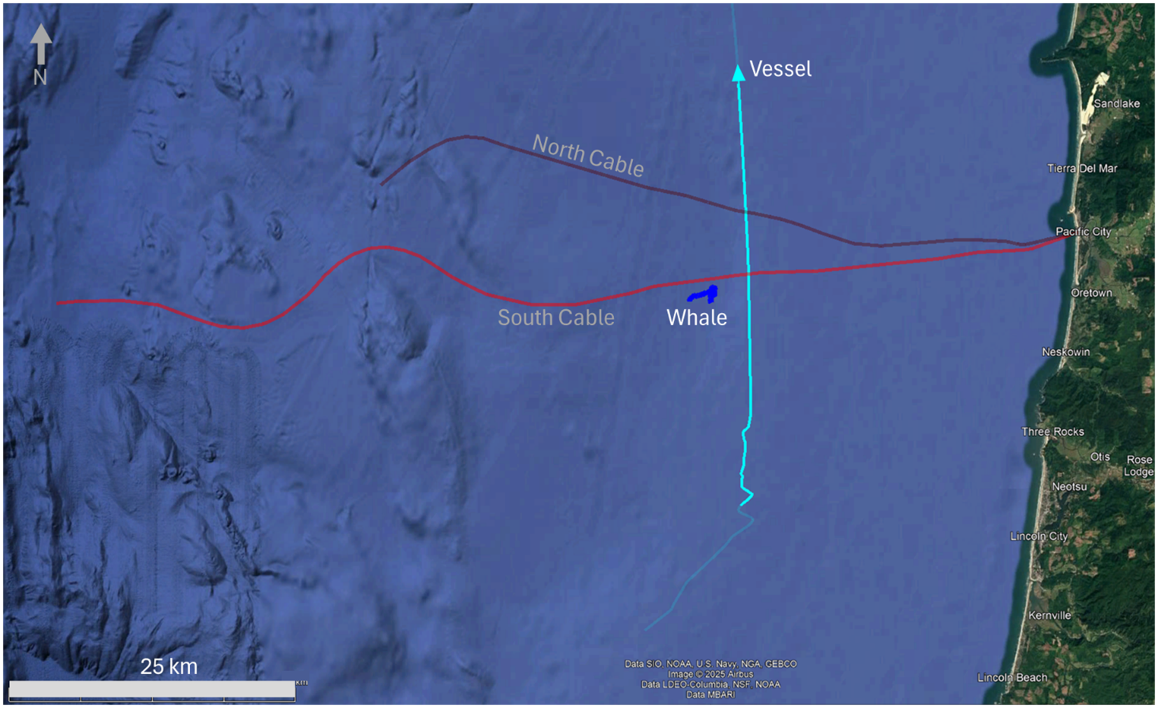
Figure 1. Map view of the study area showing the South (bright red line) and North (dark red line) cables extending into the Pacific Ocean from the Oregon coastline. Also shown are the locations of the fin whale calls analysed (dark blue line) and the track of the vessel (cyan line) (Google Earth Data SIO, NOAA, U.S. Navy, NGA, GEBCO, MBARI, LDEO-Columbia, Image ^© 2025Airbus).

An initial analysis of the RAPID OOI dataset by Wilcock et al. (2023) identified a variety of signals including blue and fin whale calls, vessel noise and ocean surface gravity waves. Subsequent studies using the data include the micro-seismicity, marine sediment characterization, ocean monitoring, and acoustic propagation (Abadi et al., 2022; Ragland et al., 2023; Douglass et al., 2023; Goestchel et al., 2024; Fang et al., 2022, Shi et al., 2025). Similar observations have also been observed in Artic regions (Bouffaut et al., 2022).

This study describes a processing scheme based on conventional earthquake analysis techniques that allowed us to identify a 2-hour long sequence of fin whale calls that coincided with the passage of a large container vessel.

2 Materials and methods

The data analysed are from the South cable and were acquired with a Silixa iDASv3 interrogator using a 30m gauge length, a channel sample spacing of 2m and a sampling frequency of 200 Hz. The fibre is interrogated up to the first optical repeater at 95km from the shore in water depths up to 1600m. Over this range the cable is buried to a nominal depth of 1.5m below the seafloor. The interrogator unit, computing equipment and data storage is located in a facility close to the beach landing point of the cable.

An early study of these data by Wilcock et al. (2023) identified many acoustic sources such as earthquakes, vessels and marine mammals, that could be used to characterize the signal and noise regimes characteristic of a submarine DAS system. Over the four days of recording earthquakes were identified, typically from far-field higher frequency T-phases (waterborne arrivals) that were effectively planar. The region offshore the Oregon coast is a busy commercial shipping area with vessels ranging from small fishing vessels (typically 20m) to much larger container and bulk carrier vessels (200 m). An analysis of public domain Automatic Identification System (AIS) data from the National Oceanic and Atmospheric Administration (NOAA) indicates that over the four days of the DAS recording 30 vessels passed within range of the sensing range of the two cables. However, only a few of the larger vessels were detectable as their Underwater Radiated Noise (URN) signatures were of higher amplitude. The vessel’s acoustic signals along with their AIS navigation data were used in calibrating the DAS channel positions along the fibre. Acoustic signals from the whales were clearly observed throughout the survey and were identified to be from blue whales and, much more frequently, fin whales (Wilcock et al., 2023).

Fin whales are some of the loudest marine animals with reported sound pressure levels (SPL) of 189 dB re 1 μPa at 1 m (Weirathmueller et al., 2012). For comparison, the SPL for an airgun array measured in horizontal directions is around 223–229 dB re 1 μPa at 1 m (Landrø and Amundsen, 2010). Typical fin whale calls last around 1s and repeat every 15 seconds with a downward frequency sweep around 20Hz. In the preliminary analysis (Wilcock et al., 2023) of the OOI RAPIDS data the fin whales were reported to be producing two call types characterized in terms of amplitude and frequency.

In the next sections we will describe how the 4 days of DAS data were screened to identify a dataset containing fin whale calls. We then used correlation techniques to generate a high-quality estimate of the call which was subsequently used to estimate direct arrival times. These arrival times were then used to the whale’s location.

2.1 Signal conditioning

The field data are dominated by slow moving, low frequency (< 1 Hz) surface gravity waves. These signals can be effectively removed using a high pass filter at e.g. 5 Hz. However, since our target signal from fin whales is band limited to frequencies between 10 and 40Hz (Wiggins and Hildebrand, 2020) we apply a 5^th order Butterworth band pass filter and additionally down-sample to 100 Hz (Nyquist frequency of 50Hz). A typical noise type associated with DAS data is so-called Common Mode Noise (CMN) which is caused by near-interrogator vibrations. CMN is characterized by instantaneous noise occurring over all channels which translates into zero-wavenumber and broadband frequency noise. This noise can be effectively removed by estimating the noise from weighted stacking across all channels and subtracting the noise estimate from the contaminated data. Finally, random noise is attenuated using a Wiener filter. At this stage we have conditioned the data so that the fin whale calls are readily visible in the data (see Figure 2).

Figure 2

Figure 2. Example of data conditioning showing 6 seconds of data from 07:16:25 UTC. The plot on the left shows the original data dominated by low frequency, low velocity surface gravity waves with a higher frequency fin whale call just visible and (right) the same data after bandpass frequency filtering, CMN removal and Wiener filtering. Trace normalization applied.

The DAS system generates significant data volumes from the four days of recording. The interrogator unit on the South cable samples data at a temporal frequency of 200Hz for over 40000 channels spaced every 2m along the cable. These sampling rates result in approximately 2.7 Tb of data being generated every day. We use a blocking approach (also known as mean pooling) to efficiently detect individual whale calls on these large data volumes. The blocking process sums the absolute strain values with blocks of size 5 channels and 5 time samples. This block size preserves the 1s long whale calls whilst reducing the data volume by a factor of 25 (see Figure 3). This blocking, in addition to the temporal down sampling from 200Hz to 100Hz, reduces the raw data volumes by a factor 50.

Figure 3

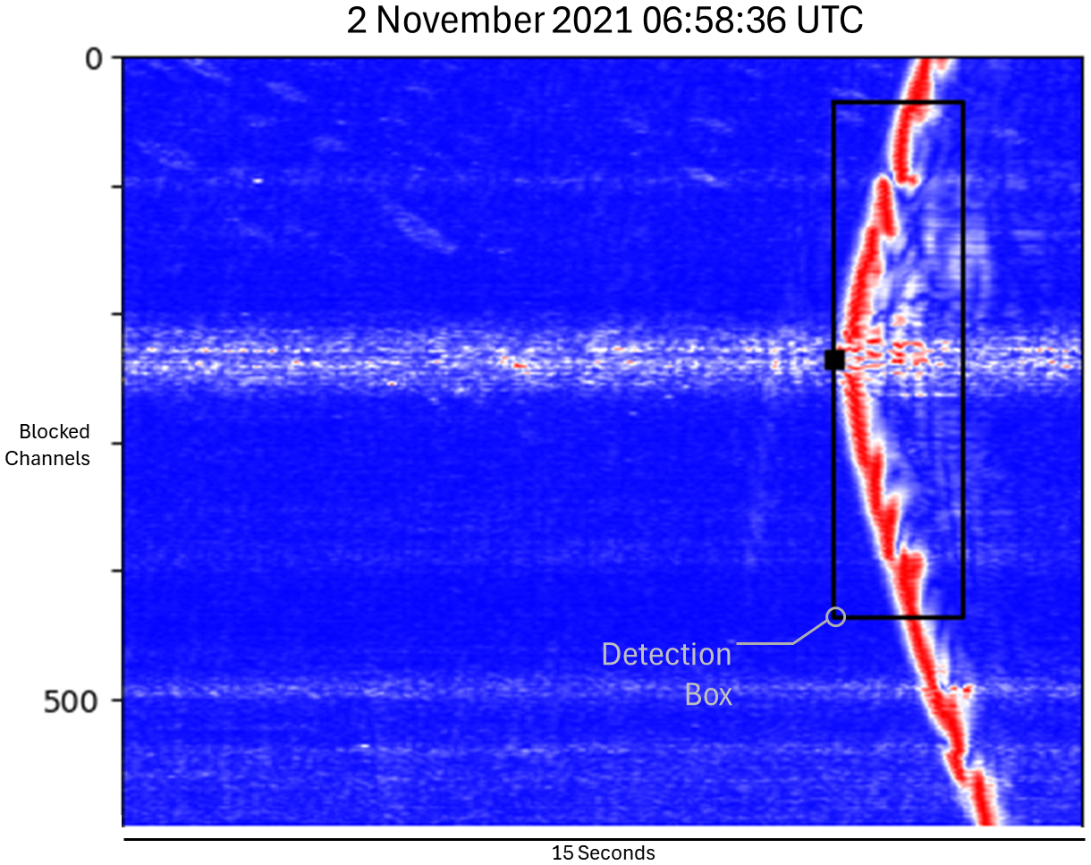
Figure 3. Detected call on blocked data at 06:58:36 UTC. The apex of the detected event is indicated by the small black square and the black outline labelled Detection Box indicates the template size.

We use template matching to detect whale calls. The templates model the whale call signature and the DAS data characteristics using amplitude and travel time modelling for events located up to 1 km offset from a linear DAS fibre (assuming 300 m water depths and a speed of sound in water of 1480 m/s). The modelling includes geometrical spreading, and the cosine squared amplitude DAS response (Mateeva et al., 2014). The resulting template corresponds to a window of spatial aperture of 4km and a temporal aperture of 2 seconds. This translates to an equivalent size of 400 channels by 40 time samples in the blocked data. From this template we also designed two additional templates – referred to as ‘Inside’ and ‘Outside’ templates - which were used to quality control (QC) detected events to remove false positives. The two QC templates are applied after a potential detection has occurred to measure the amplitudes of the data inside and outside the template, and subsequently a Signal to Noise (S/N) metric to determine the timing and type of calls was calculated (see Figure 4).

Figure 4

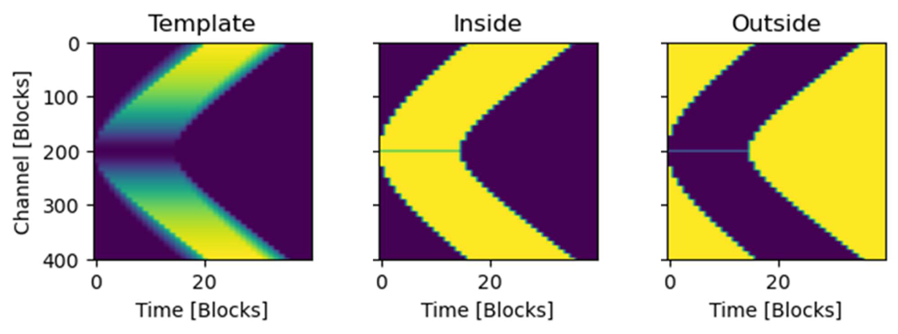
Figure 4. Detection template (left) and additional Inside (middle) and Outside (right) QC templates. Blue colours correspond to zero and yellow corresponds to 1.

The template is cross correlated with the blocked data to identify areas of high correlation. Regions exceeding a cross-correlation threshold determined from testing are then evaluated with the QC templates to obtain a signal to noise metric used to flag a valid detection. Detections are flagged when the SNR exceeds 2. Template matching is applied to data from South cable recorded on the 2 November 2021 from 06:15 to 08:15 UTC (23:15 01/11/2021 to 01:15 02/11/2021 PDT) and resulted in over 300 detections. Timeline plots showing the detection metrics of S/N and peak amplitude are shown in Figure 5. These show that the metrics generally follow two levels. Subsequent investigations show that these two levels correspond to two different call types, principally characterized by high and low amplitudes. Such calls are characteristic of fin whales and are referred to as doublet songs. We also observe breaks in the calls occurring approximately every 12 minutes and lasting for about 1 minute (as indicated by the grey boxes in Figure 5). These pauses in the calling sequences are interpreted to be the fin-whale surfacing to breath.

Figure 5

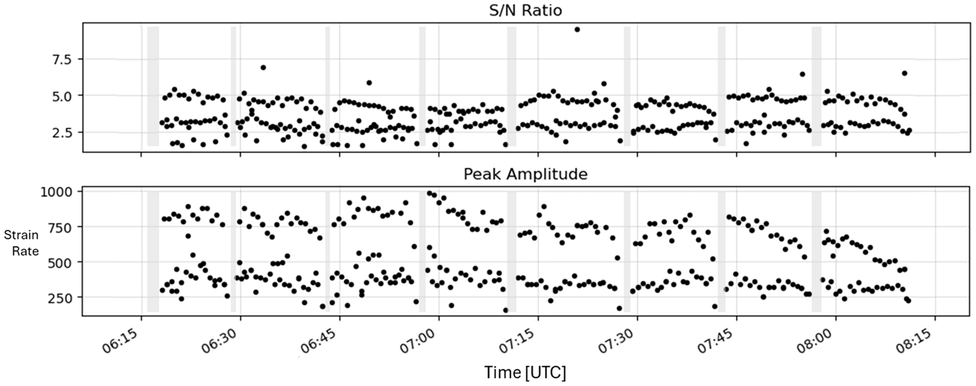
Figure 5. The top panel shows the QC metric (signal-to-noise ratio) and the lower panel shows the peak amplitude for the events detected through template matching. Grey boxes indicate time intervals where calls stop.

2.2 Localization

To locate the whale, we take the detected event and perform cross-correlation analysis between the channel waveforms and an estimate of the acoustic call waveform as a pilot trace. To start this process, we selected detections with high SNR (>3.5 and >5 respectively for the two call types) and used a single channel to obtain an initial estimate of the two call types. The cross-correlation analysis then allows the first arrivals to be aligned and stacked to obtain an improved estimate of the pilot. In the stacking procedure a robust approach is used where data exceeding a threshold correlation coefficient contribute to the stack. This cross-correlation and selective stacking yields an improved estimate of the pilot trace. This process is then repeated multiple times to obtain progressively better estimates. We use a Phase Weighted Stack (PWS; Schimmel and Paulssen, 1997) to obtain a high-quality estimate of the pilot trace (see Figure 6).

Figure 6

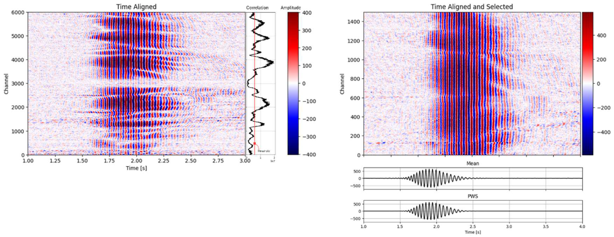
Figure 6. Direct arrivals after alignment for (left) all the channels, the computed correlation coefficients are shown in the marginal plots to the right and (right) channels exceeding a threshold in the correlation coefficients, mean (linear) and Phase Weighted Stacks (PWS) are shown below the plot.

The resulting call estimates from the cross-correlation and stacking are now characterized using analytical traces from a Hilbert transform to obtain instantaneous frequencies and amplitudes (see Figure 7). We find that the higher amplitude calls (Type 1) decrease in frequency from 27 Hz to 19 Hz over 0.65 s. The lower amplitude calls (Type 2) correspond to a down sweeping signal with frequencies decreasing from 20 to 17 Hz over 0.75s. A timeline of the call type classification from the cross-correlation is shown in Figure 8 where the 12 minutes intervals corresponding to surfacing are clearly identified.

Figure 7

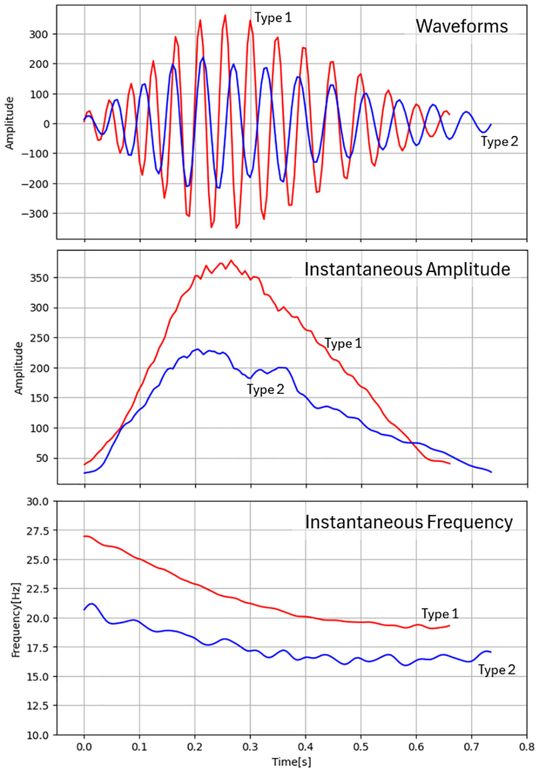
Figure 7. Pilot waveforms for the two call types observed in the data shown as red and blue lines. Top plot shows the time domain, middle plot shows the amplitude envelope, and the bottom plot shows the instantaneous frequency versus time.

Figure 8

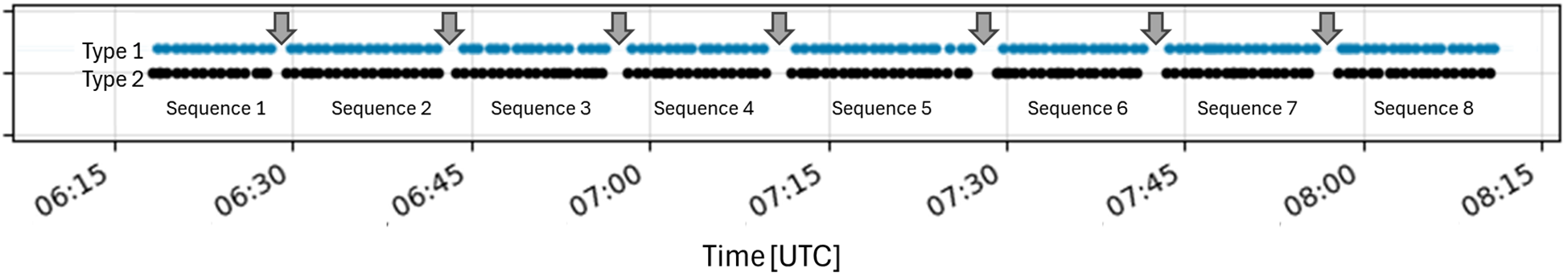
Figure 8. Timeline showing the call type classification identified through correlation analysis. The upper blue points indicate calls identified as ‘Type1’ calls. The lower black points indicate calls identified as ‘Type2’ calls. Breaks in the call sequence occur approximately every 12 minutes (indicated by grey arrows) and are interpreted to the whale surfacing to breath.

The time shifts derived from cross-correlation are used to estimate the fin whale’s location. For localization we assume the whale is 10 m below the sea surface (Kuna and Nábělek, 2021), typical for fin whales, and that the sound in water is 1480 m/s. A robust location procedure is adopted where we minimize the difference between modelled travel times and the observed travel times using a trimmed L1 metric. This metric is evaluated over a grid of potential locations where the grid minimum is then refined using a downhill gradient method (BFGS). This process of grid search followed by refinement is then repeated 3 times with each successive iteration using a smaller grid extent centred around the previous minima.

An example of the objective function for one detected event is shown in Figure 9. We can see that the objective function is bimodal with two complementary solutions located symmetrically to the North and South of the cable. These two solutions are to be expected because a uniaxial sensing linear array is unable to discriminate between these two solutions (sometimes referred to as the left-right ambiguity problem). The southern-most solution is selected based on preliminary analysis of DAS data from the North cable.

Figure 9

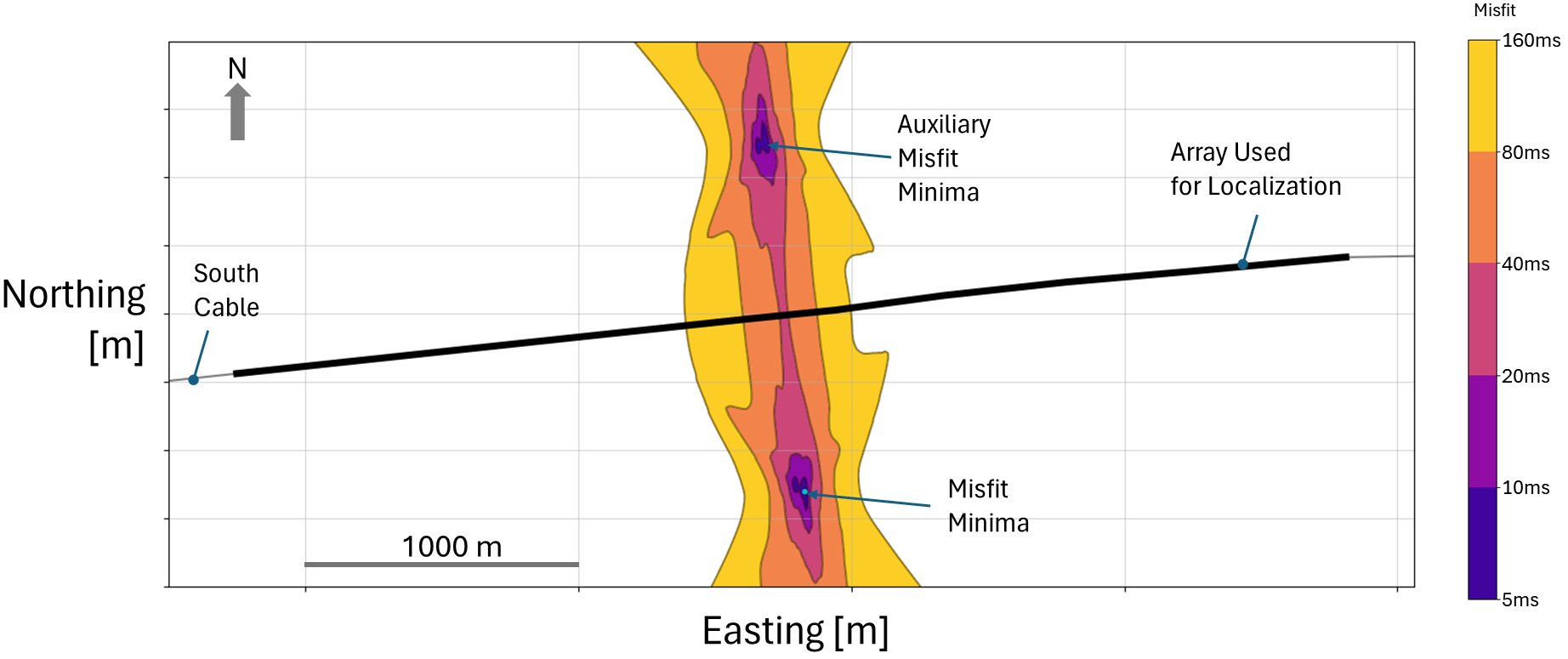
Figure 9. Example of the objective function metric used in localizing the calls showing the cable (grey line) and the portion of the cable where travel times were used in localization (thick black line).

3 Results and discussion

The location procedure is repeated for all the detected calls. We find that the whale initially follows a mostly straight track in an ENE direction nearly parallel to the South cable for approximately 2 km over 30 minutes. This translates to an average speed of 4 km/hour which compares with reported cruising speeds for fin whales of 10–15 km/hr and top speeds of 40 km/hour observed during feeding. Around 07:50 UTC the calls follow a complicated track for approximately an hour before the track moves to a SSW direction. The closest call was 750 m from the cable. The most distant call was located 2 km from the cable. The location of the calls relative to the cable are shown in Figure 10.

Figure 10

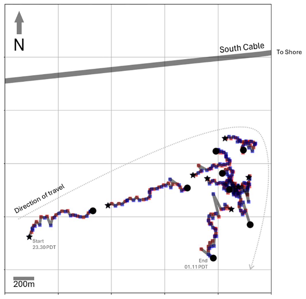
Figure 10. Map showing the located calls. High and low amplitude calls are shown as red and blue squares. The start of each sequence is indicated by a star and the end is indicates by a large black circle.

When we reviewed the detected calls, we observed that some of the calls around 07:30 UTC showed signals interpreted to be vessel noise, as shown in Figure 11. We identified this vessel by reviewing publicly available AIS data from the NOAA (National Oceanic and Atmospheric Administration) for vessels operating in this area and time frame. The acoustic signals correspond to a large container vessel of length 261 m, beam 32 m and a gross tonnage 40542 tons. Having identified the vessel, we then extracted the navigation data and time stamps over the time window where the whale calls were located. At the start of the call sequence at 06:18 UTC the vessel is located approximately 15 km to the south of the South cable and is moving slowly at ~1.5 km/hour in a NNW direction. At 06.50 UTC the vessel then starts heading directly north and accelerates to a speed of 20 km/hr over 15 minutes after which its rate of acceleration decreases until it reaches a speed of 24 km/hr at 07:40 UTC. At 07:35 UTC the vessel passes directly above the South Cable at a water depth of 370 m (see Figure 12).

Figure 11

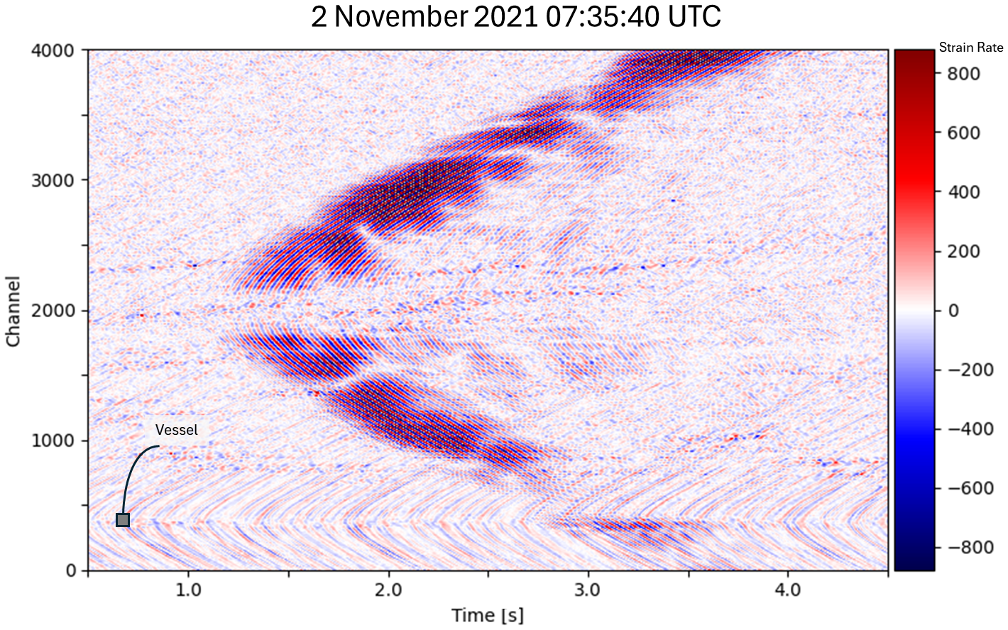
Figure 11. Acoustic strain data showing a fin whale call and vessel noise (labelled ‘Vessel’) around channel 400 at 07:35:40 UTC.

Figure 12

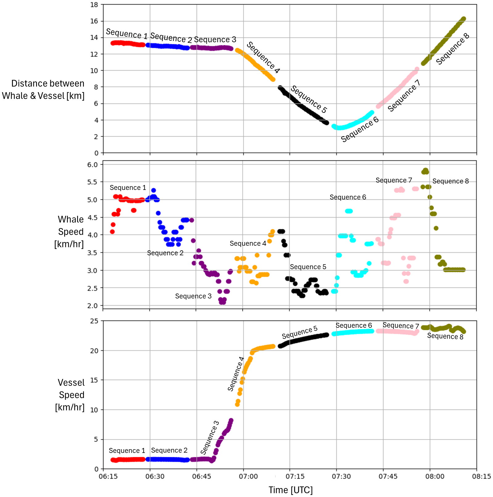
Figure 12. Timelines showing the (top) distance between the whale and the vessel, (middle) speed of the whale and (bottom) speed of the vessel. Data are coloured according to the whale call sequence.

A frequency-wavenumber (FK) analysis of the vessel reveals several tonals probably caused by engine machinery. When analysed in detail we can see that the ‘tonals’ are actually split because of Doppler effects (see Figure 13). A comparison with modelled Doppler shifts are in good agreement with the vessel speed calculated from the AIS information (Rivet et al., 2021). The FK analysis also shows dispersion signals associated with surface gravity waves and Scholte waves in the low frequency-low wavenumber region (see Figure 14).

Figure 13

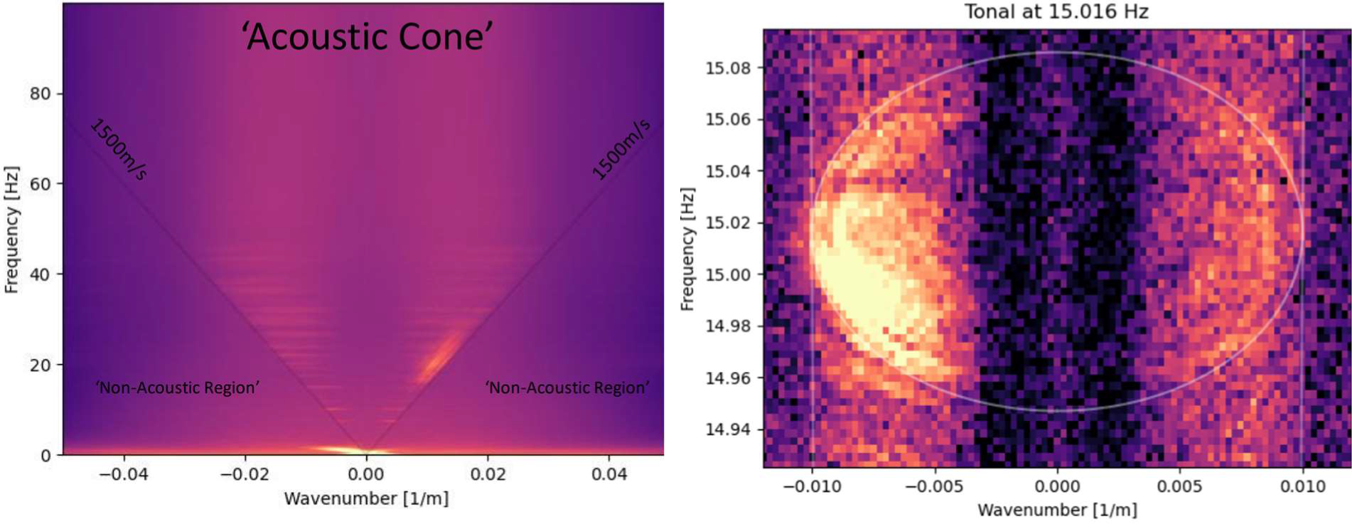
Figure 13. Average FK analysis as the vessel passes over the cable. The plot on the right is a zoom on the 15Hz tonal generated by the vessel showing the Doppler shift, the modelled Doppler shift is shown as a white ellipse.

Figure 14

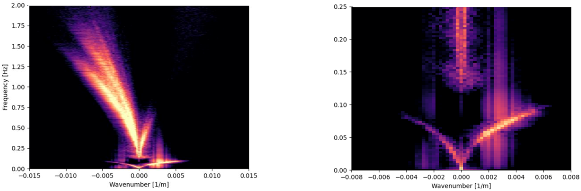
Figure 14. Average FK Analysis in the low frequency low wavenumber region showing (left) Scholte waves and (right) surface gravity waves.

We suggest that there is a behavioural response by the whale to the vessel. As the vessel starts to accelerate and move northwards at 06:50 UTC - during Sequence 3 - the whale slows down to a minimum speed of 2 km/s and moves in a NW direction, away from the vessel located 13 km to the SSE. Prior to this time, for sequences 1 and 2, the whale was proceeding east towards the coastline. During sequences 4 to 7 the whale calls seem to follow a complicated trajectory and generally moves more slowly whilst the distance between the whale and the vessel decreases from 10 km to a closest approach distance of 3 km. In the final sequence (Sequence 8) the whale starts to follow a more linear southwards direction away from the north bound vessel. These interactions are summarized in Figure 12 & Figure 15. Whilst we have suggested that the whale’s behavioural response is in response to the vessel it could also be related to feeding or other behaviours. To establish typical behavioural responses would require datasets acquired over longer time frames. Nonetheless, such avoidance behaviours by whales has previously been reported in the Bay of Biscay in relation to fast ferries in the Bay of Biscay (Aniceto et al., 2016), seismic airguns (Caruso et al., 2016) and military exercises (Thomas and Martin, 2021). It may also be possible to identify subtle changes in vocalization characteristics that may also be indicative of avoidance behaviour (e.g. Caruso et al., 2016).

Figure 15

Figure 15. Map showing (left) the located calls in relation to the vessel track where the track is colour coded to correspond with the call sequence. The plot on the right is a close-up view of the whale call locations.

4 Conclusions

We have shown how DAS data acquired on an existing telecommunications fibre can be analysed to investigate the response of fin whales located within 2km of the seabed cable. Through an application of conventional earthquake processing techniques e.g. template matching, travel time location, and signal processing techniques e.g. correlation, stacking, instantaneous attributes etc., we can track a fin whale over a period of 2 hours and acoustically characterize the calls. We find that the calls form a doublet song principally characterized by amplitude and frequency. Over the course of 2 hours, we see distinct breaks in the call sequence that occur approximately every 12 minutes. These breaks are interpreted to be when the fin whale surfaces to breath. We found that the whale initially moved eastwards but then abruptly changes its behaviour to a more chaotic behaviour before proceeding southwards. We investigated this further and found that the time period of erratic behaviour was coincident with the passage of a northbound large container vessel. Whilst such behaviours have been previously observed the non-uniqueness associated with the location method limits this conclusion. These location ambiguities can be resolved if the cable deviates from a line array, or in other words the cable curves. Nonetheless, this study shows that DAS can be used to understand the behavioural responses of marine wildlife and commercial activities. Furthermore, a real time monitoring solution to prevent ship strikes is feasible since the data volumes and processing loads are similar to those used for real time seismic monitoring applications e.g. geothermal, carbon sequestration (e.g. Mondanos et al., 2024). DAS can contribute to existing Passive Acoustic Monitoring (PAM) systems (e.g. buoys, gliders, towed arrays) and have the advantage of offering a long-range monitoring solution that can be retrofitted to existing offshore telecommunication fibres.

Data availability statement

Publicly available datasets were analysed in this study. This data can be found here: https://doi.org/10.58046/5J60-FJ89.

Ethics statement

Ethical approval was not required for the study involving animals in accordance with the local legislation and institutional requirements because observation of animals in the natural environment with a non-invasive sensing system.

Author contributions

SH: Conceptualization, Data curation, Formal Analysis, Investigation, Methodology, Software, Supervision, Validation, Visualization, Writing – original draft, Writing – review & editing. AS: Conceptualization, Formal Analysis, Funding acquisition, Investigation, Methodology, Project administration, Supervision, Writing – review & editing. FS: Conceptualization, Data curation, Formal Analysis, Investigation, Methodology, Validation, Writing – review & editing.

Funding

The author(s) declare that financial support was received for the research and/or publication of this article. Work funded by Silixa Ltd.

Acknowledgments

We gratefully acknowledge the use of the AIS and Oregon RAPID OOI open-source datasets (Wilcock and Ocean Observatories Initiative, 2023). Preliminary data preparation was performed for the UKAN Underwater Acoustics Data Challenge Workshop 2023.

Conflict of interest

Authors Authors SH, AS, and FS were employed by the company Silixa Ltd.

The authors declare that this study received funding from Silixa Ltd. The funder had the following involvement in the study: data collection and analysis, decision to publish, and preparation of the manuscript.

Generative AI statement

The author(s) declare that no Generative AI was used in the creation of this manuscript.

Publisher’s note

All claims expressed in this article are solely those of the authors and do not necessarily represent those of their affiliated organizations, or those of the publisher, the editors and the reviewers. Any product that may be evaluated in this article, or claim that may be made by its manufacturer, is not guaranteed or endorsed by the publisher.

References

Abadi S., Wilcock W., and Lipovsky B. (2022). Detecting hydro-acoustic signals using Distributed Acoustics Sensing technology. J. Acoust. Soc Am. 152, A201. doi: 10.1121/10.0016027

Crossref Full Text | Google Scholar

Aniceto A., Carroll J., Tetley M., and van Oosterhout C. (2016). Position, swimming direction and group size of fin whales (Balaenoptera physalus) in the presence of a fast-ferry in the Bay of Biscay. Oceanologia 58, 235–240. doi: 10.1016/j.oceano.2016.02.002

Crossref Full Text | Google Scholar

Bouffaut L., Taweesintananon K., Kriesell H., Rørstadbotnen R., Potter J., Landro M., et al. (2022). Eavesdropping at the speed of light: distributed acoustic sensing of baleen whales in the arctic. Front. Mar. Sci. 9. doi: 10.3389/fmars.2022.901348

Crossref Full Text | Google Scholar

Caruso F., Lizarralde D., Elsenbeck J., Collins J., Zimmer W., and Sayigh L. (2016). Detection and tracking of fin whales during seismic exploration in the Gulf of California. Proc. Meetings Acous.: Fourth Intern. Conf. Eff. Noise Aquat. Life 27, 070021. doi: 10.1121/2.0000424

Crossref Full Text | Google Scholar

Douglass A., Ragland J., and Abadi S. (2023). Overview of distributed acoustic sensing technology and recently acquired data sets. J. Acoust. Soc Am. 153, A64. doi: 10.1121/10.0018174

Crossref Full Text | Google Scholar

Fang J., Williams E., Yang Y., Biondi E., and Zhan Z. (2022). “Unraveling the distribution of microseism sources with submarine distributed acoustic sensing,” in AGU Fall Meeting. Chicago, Illinois. Abstr. S52C–0077.

Google Scholar

Goestchel Q., Wilcock B., and Abadi S. (2024). Automated detection of fin whale calls recorded with distributed acoustic sensing. J. Acoust. Soc Am. 155, A133. doi: 10.1121/10.0027063

Crossref Full Text | Google Scholar

Kuna V. and Nábělek J. L. (2021). Seismic crustal imaging using fin whale songs. Science 371, 731–735. doi: 10.1126/science.abf3962

PubMed Abstract | Crossref Full Text | Google Scholar

Landrø M. and Amundsen L. (2010). Marine Seismic Sources Part I (London: GeoExpro, Geopublishing Ltd,).

Google Scholar

Mateeva A., Lopez J., Potters H., Mestayer J., Cox B., and Kiyashchenko D. (2014). Distributed acoustic sensing for reservoir monitoring with vertical seismic profiling. Geophys. Prosp. 62, 679–692. doi: 10.11111/1365-2478.12116

Crossref Full Text | Google Scholar

Mondanos M., Marchesini P., Stork A., Maldaner C., Naldrett G., and Coleman T. (2024). A distributed fibre-optic sensing monitoring platform for CCUS. First Break. 42, (3) 77–(3) 83. doi: 10.3997/1365-2397.fb2024026

Crossref Full Text | Google Scholar

National Oceanic and Atmospheric Administration. Available online at: coast.noaa.gov/digitalcoast/tools/ais.html (Accessed October 20, 2024).

Google Scholar

Ragland J., Douglass A., and Abadi S. (2023). Using distributed acoustic sensing for ocean ambient sound analysis. J. Acoust. Soc Am. 153, A64. doi: 10.1121/10.0018176

Crossref Full Text | Google Scholar

Rivet D., de Cacqueray B., Sladen A., Roques A., and Calbris. G. (2021). Preliminary assessment of ship detection and trajectory evaluation using distributed acoustic sensing on an optical fiber telecom cable. J. Acoust. Soc Am. 149, (4) 2615–2627. doi: 10.1121/10.0004129hal-03209679f

PubMed Abstract | Crossref Full Text | Google Scholar

Schimmel M. and Paulssen H. (1997). Noise reduction and detection of weak, coherent signals through phase weighted stacks. Geophy. J. Int. 130, 497–505. doi: 10.1111/j.1365-246X.1997.tb05664.x

Crossref Full Text | Google Scholar

Shi Q., Williams E., Lipovsky B., Denolle M., Wilcock W., Kelley D., et al. (2025). Multiplexed distributed acoustic sensing offshore central oregon. Seismol. Res. Let 96, 784–800. doi: 10.1785/0220240460

Crossref Full Text | Google Scholar

Thomas L. and Martin S. (2021). Changes in the movement and calling behavior of minke whales (Balaenoptera acutorostrata) in response to navy training. Front. Mar. Sci. 8. doi: 10.3389/fmars.2021.660122

Crossref Full Text | Google Scholar

Weirathmueller M., Wilcock W., and Soule D. (2012). Source levels of fin whale 20 Hz pulses measured in the Northeast Pacific Ocean. J. Acoust. Soc Am. 133, 741–749. doi: 10.1121/1.4773277

PubMed Abstract | Crossref Full Text | Google Scholar

Wiggins S. and Hildebrand J. (2020). Fin whale 40-Hz calling behavior studied with an acoustic tracking array. Mar. Mam. Sci. 36, (3) 964–971. doi: 10.1111/mms.12680

Crossref Full Text | Google Scholar

Wilcock W., Abadi S., and Lipovsky. B. (2023). Distributed acoustic sensing recordings of low-frequency whale calls and ship noise offshore Central Oregon. J. Acoust. Soc Am. Exp. Let. 3, 026002. doi: 10.1121/10.0017104

PubMed Abstract | Crossref Full Text | Google Scholar

Wilcock W. and Ocean Observatories Initiative (2023). Rapid: A community test of distributed acoustic sensing on the ocean observatories initiative regional cabled array [Data set]. Ocean Observ. Initiat. doi: 10.58046/5J60-FJ89

Crossref Full Text | Google Scholar