Abstract
Marine heatwaves (MHWs) adversely impact Aotearoa New Zealand’s marine ecosystems and pose challenges for resource management. In this study, we evaluate forecast skill of monthly MHWs and sea surface temperature (SST) anomalies using a multi-model ensemble (MME) comprised of nine general circulation models and 206 members with a focus on Aotearoa New Zealand for the first time. Over the hindcast period (1993–2016), the MME outperforms individual models in forecasting SST anomalies around Aotearoa New Zealand, based on its higher anomaly correlation coefficient (ACC) and lower root mean square error (RMSE). The forecast skill of the MME varies seasonally, and is highest for forecasts initialized between June and September and lowest from October to December. Forecasts generally outperform persistence across all months and lead times, except at certain lead times between September and December. The background climate state also influences the MME skill, with higher accuracy during El Niño for forecasts initialized from December to February and during La Niña for certain lead times from March to August. Skill improves in spring under neutral (normal) conditions. We also evaluate the MME’s skill in predicting MHW events using a probabilistic framework. The MME retains skill up to two months along Aotearoa New Zealand’s western coast and upper east North Island but has negligible skill at four- and five-month lead times. Overall, these findings highlight that MHW and SST can be forecasted with reliability, especially at one and two months of lead time with important implications for marine resource management.
1 Introduction
Marine heatwaves (MHWs) are distinct and extended periods of unusually warm water that have caused significant alterations in marine ecosystems and the services they offer (e.g. fisheries and aquaculture Hobday et al., 2016; Oliver et al., 2018, 2019; Smith et al., 2021). These events have increased in frequency, duration, and intensity over the past century (Oliver et al., 2018; Holbrook et al., 2019). This pattern is expected to intensify with future climate change (Behrens et al., 2022; Cornelissen et al., 2025), potentially driving many marine species and ecosystems to the brink of their thermal endurance (Oliver et al., 2019; Smale et al., 2019; Cheng et al., 2025), including in the coastal zone (Thoral et al., 2022) where a significant part of aquaculture occurs (Primavera, 2006).
Marine organisms, including commercially valuable species, are highly sensitive to changes in ocean temperature, and therefore MHWs have been associated with aquaculture loss globally (Smith et al., 2021) and throughout Aoteroa New Zealand (Broekhuizen et al., 2021; Rampal et al., 2023; Montie et al., 2024; Cook et al., 2024; Cheng et al., 2025). Mussel aquaculture in the Pelorus Sound is more productive under cooler sea surface temperature (SST) (Zeldis et al., 2013), while higher sea surface temperature anomalies (SSTA) tend to reduce mussel yields (Rampal et al., 2023). Farming of Chinook salmon (Oncorynchus tshawytscha) has also suffered with reduced productivity and higher mortality rates due to recent MHWs (Cook et al., 2024). Knowledge of future SST conditions is particularly important for Aoteroa New Zealand’s aquaculture sector, which generated NZD$ 600 million in sales in 2018 and has grown by an average of 7% annually since 2012. In addition, the sector aims to increase its sales to NZD$ 3 billion by 2035 (Ministry for Primary Industries, 2023). Thus, understanding and predicting MHWs is therefore an important challenge for climate science and marine resource management (Spillman et al., 2025).
Seasonal to sub-seasonal SST forecasts, generated using coupled ocean-atmosphere general circulation models (GCMs), offer a means to anticipate these events and provide early warnings (Jacox et al., 2022; Stevens et al., 2022). The ocean-atmosphere coupling between these models is essential for capturing large-scale ocean-atmosphere variability and interactions, such as Western Boundary Current variabilities (e.g. Santana et al., 2021), the Indian Ocean Dipole and El Niño-Southern Oscillation (ENSO), which are crucial for predictability at monthly to seasonal timescales (Bi et al., 2013; Chaudhari et al., 2013; Johnson et al., 2019; Wedd et al., 2022; Rampal et al., 2023; Hobeichi et al., 2024). In addition, the skill of seasonal forecasts can vary with the background climate state. For instance, de Burgh-Day et al. (2022) found that SST anomaly forecast skill around Aotearoa New Zealand depends on the season of initialization. Additionally, Jacox et al. (2022) found that MHW forecast skill depends on the season of initialization, and showed that global MHW forecasts have a higher accuracy during active ENSO phases (El Niño and La Niña).
Multi-model ensemble (MME) combines forecasts from multiple independent GCMs and have been shown to outperform single models in seasonal prediction by reducing systematic biases and enhancing skill (Hagedorn et al., 2005; Fauchereau et al., 2022; Jacox et al., 2022). This MME approach accounts for both initial condition uncertainty and structural model uncertainty, leading to more reliable probabilistic forecasts (Chaudhari et al., 2013; MacLachlan et al., 2015a) and a better representation of uncertainty in a seasonal forecast (Hagedorn et al., 2005; Fauchereau et al., 2022). Previous evaluations of MHW forecasts focused on Aotearoa New Zealand have often utilized ensembles from single coupled models (e.g. de Burgh-Day et al., 2022), limiting the assessment of model structural uncertainty.
In this study, we assess the forecast skill of a MME comprising nine GCMs and 206 ensemble members in predicting SST anomalies and MHWs around Aotearoa New Zealand, with lead times of up to five months. Our analysis focuses on five key aquaculture regions: Coromandel, Ōpōtiki Golden Bay, Pelorus Sound (near entrance region), and Foveaux Strait (Figure 1). We evaluate (i) deterministic forecast performance using anomaly correlation coefficients (ACC) and root mean square error (RMSE), and (ii) probabilistic MHW forecast skill using the Symmetric Extremal Dependence Index (SEDI) (Ferro and Stephenson, 2011; Jacox et al., 2022). In addition, we explore seasonal variations in forecast skill, the influence of ENSO phases (El Niño, La Niña, and Neutral), and spatial differences across coastal regions.
Figure 1
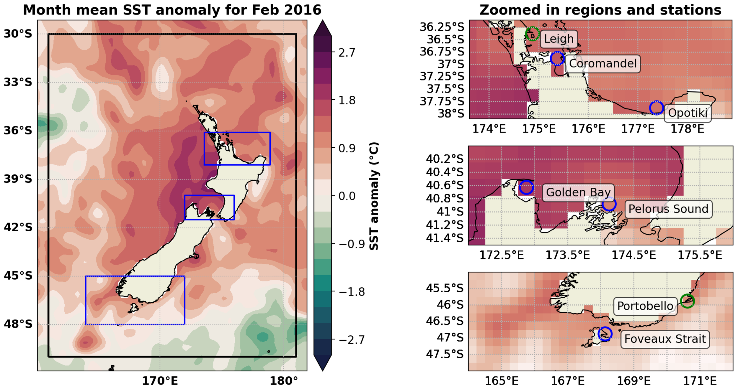
Monthly mean Sea Surface Temperature (SST) anomaly in February 2016 (left panel) highlighting the study area around Aotearoa New Zealand (black rectangle) and coastal regions (blue rectangles). Each SST grid point (blue circles in the right panels) mark the selected grid points used for multi-model ensemble (MME) assessment near aquaculture regions in Coromandel and Ōpōtiki (top right), Golden Bay and Pelorus Sound (centre right), and Foveaux Strait (bottom right). The green circles highlight Leigh (top right) and Portobello (bottom right) coastal stations with long-term in situ measurements that were used for validation of the MME forecast.
This study builds on previous work by offering a regionally focused evaluation with direct relevance to aquaculture operations in Aotearoa New Zealand. It differs from Jacox et al. (2022) and de Burgh-Day et al. (2022) by employing a larger ensemble of publicly available models, stratifying forecast performance by ENSO phase, and targeting specific aquaculture zones. While we acknowledge that monthly temporal resolution and 0.25° spatial resolution are not ideal for resolving fine-scale coastal variability, previous studies have shown that low-resolution satellite SST products compare well with in situ observations in Aotearoa New Zealand’s coastal waters (e.g. Shears and Bowen, 2017; Chiswell and Grant, 2018; Montie et al., 2024). Nevertheless, we also evaluate the MME SST forecast against in situ data from two coastal stations: Leigh and Portbello (Shears and Bowen, 2017; Cook et al., 2022) (Figure 1). Our findings support the use of MME forecasts as a valuable early-warning tool in regions with a relatively high connectivity with the nearby ocean and/or as boundary input for higher-resolution regional models.
2 Methods
2.1 Observational datasets
We used the Optimum Interpolation Sea Surface Temperature (OISST) v2.1 observational dataset produced by NOAA (Huang et al., 2021). This product is available at 1/4° of spatial resolution and at a daily frequency. OISST is treated as ground truth and is used to evaluate the SST anomalies and MHW forecasts in this study. OISST integrates observations from satellites, ships, buoys, and Argo floats onto a grid, and accounts for platform variations and sensor biases (Huang et al., 2021). Shears and Bowen (2017) compared OISST and in situ datasets from 1982 to 2016 in different coastal regions of Aotearoa New Zealand, including estuarine stations, and found high correlation coefficients (0.66–0.81). The OISST data used in this study is subset around Aotearoa New Zealand 30-50°S, and 161-181°W. This region is illustrated as a black rectangle in Figure 1.
In addition to satellite-derived SST data, we evaluated the MME forecast skill using in situ SST anomaly observations from two long-term coastal monitoring stations: Leigh and Portobello (Shears and Bowen, 2017; Cook et al., 2022). Leigh is located at the entrance of Hauraki Gulf and is more exposed to offshore conditions, whereas Portobello is situated within Otago Harbour, a narrow and shallow estuarine system with limited oceanic exchange (Figure 1). We anticipate that correlations between the MME and Portobello data will be negatively impacted by the lack of estuarine representation in GCMs. Daily SST in situ measurements have been collected at 9:00 AM at the sites since 1967 (Leigh) and 1953 (Portobello), initially through manual sampling and, since the early 2000s, via automated electronic sensors. For consistency with the model output, the in situ data were aggregated to monthly means and converted to anomalies by subtracting the monthly climatology over the hindcast period. Linear de-trending was applied to all SST anomaly observations and model outputs to reduce the effect of temperature trends on model evaluation and MHW analysis (Smith et al., 2025).
This study used the Niño 3.4 index to assess how MME forecast skill varies across ENSO phases. El Niño months are defined as those with sea surface temperature (SST) anomalies in the central Pacific derived from a 5-month centred running mean exceeding 0.5°C, while La Niña months are defined as those with SST anomalies below -0.5°C, all other months between –0.5, and 0.5°C are defined as neutral. These indices were obtained from NOAA (https://psl.noaa.gov/data/correlation/nina34.anom.data, last access on 7th of April 2025).
2.2 Multi-Model Ensemble
When assessing ensemble monthly forecasts, we evaluated the hindcast period spanning from 1993 to 2016. The hindcast involves running a GCM retrospectively using “true” initial conditions typically derived from reanalysis data. In contrast, forecasts are operational runs that utilize a slightly varied data assimilation configuration, usually using a more limited amount of observational data. Since the hindcast uses initial conditions from reanalysis data, which incorporate more observations than operational forecasts, it likely represents an upper bound on the forecast skill. While the hindcast period (1993–2016) aligns with Copernicus standards and previous studies (e.g. Jacox et al., 2022; de Burgh-Day et al., 2022), we acknowledge that extending the analysis to include operational forecasts post-2016 could offer additional insights into model evolution and real-time applicability. This will be explored in future work.
The monthly hindcast outputs are sourced from the Copernicus Climate Data Store (CDS), established under the auspices of the Copernicus Climate Change Service (C3S). The CDS collects hindcast and forecast data generated by nine international institutions, namely the European Centre for Medium-Range Weather Forecasts (ECMWF), the United Kingdom Meteorological Office (UKMO, UK), Météo-France (the French Meteorological agency), The Deutscher Wetterdienst (DWD, Germany), the Centro Euro-Mediterraneo sui Cambiamenti Climatici (CMCC, Italy), the National Centers for Environmental Prediction (NCEP, USA), the Japan Meteorological Agency (JMA, Japan), and Environment and Climate Change Canada (ECCC) which has two GCMs: ECCC-CanCM4i and ECCC-GEM5-NEMO. Together, these GCMs constitute the multi-model ensemble (MME). The period covering from 1993 to 2016 is considered standard by C3S and it is used in several studies (e.g. Lledó et al., 2020; Thornton et al., 2023).
The coarse resolution (1°) SST fields from all GCMs are interpolated to the observational grid (0.25°), with land pixels as defined in the observational dataset removed. Linear de-trending was also applied to the individual members of each GCM. In total, there are 206 ensemble members in the MME (across nine models). A brief summary about the GCMs used in this study is presented in Table 1.
Table 1
| Originating institution | General circulation model | Ensemble size | Reference |
|---|---|---|---|
| ECMWF | SEAS5 | 25 | Johnson et al. (2019) |
| UKMO | GloSea6-GC3.2 | 28 | MacLachlan et al. (2015b) |
| Météo -France | Météo –France System 8 | 25 | Patterson et al. (2025) |
| DWD | GCFS 2.1 | 30 | Deutscher Wetterdienst (2020) |
| CMCC | CMCC-SPS3.5 | 40 | Sanna et al. (2017) |
| NCEP | CFSv2 | 28 | Saha et al. (2014) |
| JMA | JMA/MRI-CPS3 | 10 | Hirahara et al. (2023) |
| ECCC | CanCM4i | 10 | Lin et al. (2020) |
| ECCC | GEM5-NEMO | 10 | Lin (2020) |
Characteristics of the general circulation models (GCMs) constituting the multi-model ensemble.
2.3 Deterministic forecast validation
In this study, we evaluate the skill of SST anomaly forecasts in nine GCMs during the hindcast period (1993-2016). The GCM forecast are initialised around the 1st and the simulations are made available around the 15th of each month. We downloaded the forecasted SST data from one to five months of lead time. For each GCM, we first compute a lead-time-dependent climatology of SST across all ensemble members, spanning 1993–2016. SST anomalies are then calculated relative to these climatologies for each GCM member. The ensemble members for each GCM are averaged to generate a deterministic prediction of SST anomalies from each originating institution (e.g. ECMWF, Table 1). Additionally, we compute a multi-model ensemble (MME) mean by averaging all members of the deterministic forecasts from each GCM following Jacox et al. (2022).
The skill of SST forecasts is evaluated using two metrics: the anomaly correlation coefficient (ACC) and the root mean squared error (RMSE). ACC and RMSE are defined as:
where observed (x) and predicted (y) SST anomalies are compared at the same time and space (i=1,2,…,n) and against averages (−) also applied in time and space, in the case of ACC (Figure 2). In addition, we calculate the ACC (Equation 1) per month using spatial data (Figure 3). We use 1-month lead time forecasts to calculate the spatial correlation with observations and compare that with the ENSO index.
Figure 2

Anomaly correlation coefficient (ACC, left – larger values indicate more skill), and root mean square error (RMSE, right – smaller values indicate more skill) of SST anomaly forecast over the Aotearoa New Zealand from 1993 to 2016. The black solid line represents the multi-model ensemble (MME) mean, while coloured lines denote individual models. The red dashed line corresponds to a persistence forecast.
Figure 3
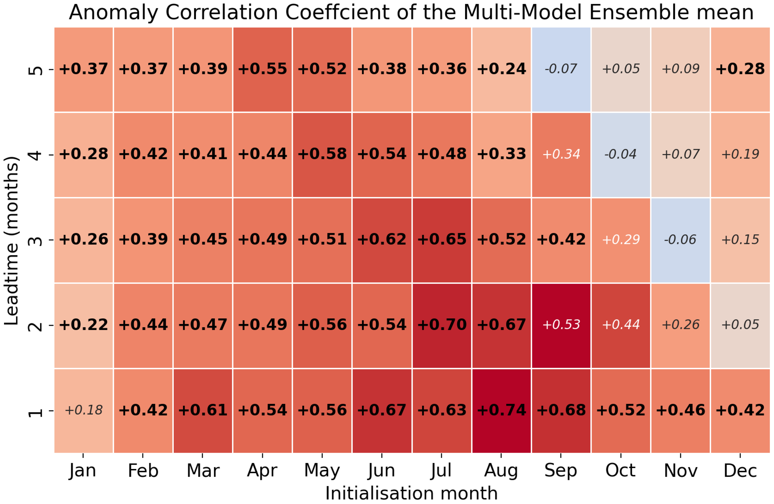
Multi-model ensemble (MME) mean sea surface temperature (SST) anomaly correlation coefficient (ACC) per month and per lead time (month). The ACC is calculated between anomaly SST from OISST and the MME mean. Bold numbers represent ACC larger in the MME mean compared to the persistence ACC. Non-bold numbers represent the opposite.
The RMSE (Equation 2) of model SST anomaly quantifies the overall magnitude of forecast errors by measuring the average deviation between predicted and observed SST values. The ACC is a dimensionless metric ranging from -1 to 1 that evaluates the agreement between forecasted and observed anomalies by correlating their anomalies. Here, the ACC is computed across all forecast initialization times and all spatial locations (latitudes and longitudes), thus evaluating the temporal and spatial consistency of the forecasts. The ACC is also computed as a function of season and ENSO index.
The deterministic forecasts are also evaluated against a persistence baseline. A persistence forecast uses observed SST anomaly of the previous month (1st to the ∼30th) which is ∼15 days earlier compared to the same time as the forecasts are available. In an operational setting, this is more realistic because the next ∼15 days future of observations are not available to compute the monthly mean SST. For instance, a February MME forecast initialised on January 1st is compared to a persistence forecast also generated on January 1st using December’s (1st to the ∼30th) mean anomaly. The persistence baseline used here assumes that SST anomalies remain constant from the previous month, a method commonly used in seasonal forecast benchmarking (e.g. Jacox et al., 2022).
2.4 MHW forecast evaluation
MHWs are defined as a period of warm ocean temperatures that exceed the 90th percentile of local historical temperatures for that specific time of the year for at least five days (Hobday et al., 2016). In this work, we analyse monthly averages SST anomalies, therefore we use an adapted version of the MHW definition which was proposed by Jacox et al. (2022). They define MHW months as those when SSTs exceed the 90th percentile for a given month based on a climatology (e.g. 1993–2016 period). Due to the monthly resolution of the forecast data, our MHW definition does not capture short-duration events. This limitation is acknowledged and discussed further in Section 4.
We evaluate month-mean forecasts of MHW events using both the MME mean (deterministic approach) and a probabilistic approach (Jacox et al., 2022). The deterministic approach uses the MME mean and climatological 90th percentiles to define thresholds that characterise MHW events. On the other hand, the probabilistic method uses individual ensemble members and their specific 90th percentiles. A binary forecast is derived for each member (0 = below 90th percentile, 1 = equal or above the 90th percentile) and the probability of a MHW to occur is then calculated as the average of these binary forecasts across all ensemble members of the multi-model ensemble (206 members for the hindcast period).
The probabilistic MHW forecast fall anywhere between zero and one, and an additional threshold (e.g. 0.2 or 20%) is needed (or selected by individual decision-makers) to determine the presence or not of a MHW event per forecasted grid point. The use of this threshold allows for the binary re-classification of the probabilistic forecast and for later evaluation. The probabilistic MHW differs from the deterministic MHW forecast by providing the likelihood of MHW event to occur which assists decision-making by forecast users.
To evaluate the skill of MHW events produced by the MME mean (deterministic) and the probabilistic MHW forecast, we use the symmetric extremal dependency index (SEDI) (Ferro and Stephenson, 2011). The SEDI is defined as:
where F is the false alarm rate (ratio of false positives to total observed non-events) and H is the hit rate (ratio of true positives to total observed events). H = TP/(TP+FN) in which TP represents the total of true positives and FN the total of false negatives given a selected probability threshold (e.g. 0.2). F = FP/(FP+TN), FP is the total of false positives and TN represents the total of true negatives (Ferro and Stephenson, 2011). We calculate the SEDI (Equation 3) for different probability thresholds: 0.05, 0.1, 0.2, and 0.3 (not shown), to determine MHW events and evaluate the probabilistic MHW forecast. SEDI scores range from -1 (no skill) to 1 (perfect skill), and scores above (below) zero indicate forecasts that are better (worse) than random chance.
3 Results
3.1 General SST anomaly forecast evaluation
Statistical evaluation of the multi-model ensemble (MME) mean demonstrates consistently higher skill in forecasting SST anomalies around Aotearoa New Zealand in comparison with that of any individual coupled model (Figure 2). Over the 1993–2016 period, the MME mean ACC is greater than any individual GCM mean at lead times of one to five months. This result aligns with the well-established rationale that combining models tends to improve seasonal forecast skill by averaging out individual model errors (Hagedorn et al., 2005). We also find that the persistence forecast of SST anomalies (observation from the previous month) is worse than that of any single GCM at lead times beyond one month.
The MME root mean square error (RMSE) increases with lead time, indicating growing forecast uncertainty (right panel in Figure 2). However, the MME consistently achieves lower RMSE values compared to any individual GCM, with errors starting around 0.50°C at one-month lead time and rising to approximately 0.55°C at five-month lead time. A RMSE of ∼0.5°C is comparable to regional reanalyses SST errors (e.g. Santana et al., 2020, 2023). The persistence forecast exhibits the highest RMSE, exceeding 0.70°C at longer lead times. Overall, these results demonstrate the advantage of multi-model ensembles in SST forecasting, yielding improved correlation and reduced error compared to individual models and persistence forecasts.
The decomposition of the ACC as a function of initialisation month shows that there is strong seasonality in forecasting skill (Figure 3). In general, the MME is more skillful than the persistence forecast across most months and lead times (bold numbers in Figure 3). The ACC of the MME mean tends to be greatest for forecast initialized between June to September, when ACCs are greater than 0.6 for lead time of one month and greater than 0.4 for lead times between one and three months. From October to December, the MME mean skill decreases for lead times greater than one month and is outperformed by a persistence forecast. February SST anomalies are the hardest to predict. Forecasts initialised in September (5-month lead time) and January (1-month lead time) have the lowest ACCs for the period analysed. This lower ACC for February also occurs for forecasts initialised between October and December. Forecast skill, however, with lead time longer than a month, starts to improve again from January onwards, when the ACC exceeds 0.4 in February.
3.2 Influence of ENSO on forecast skill
The ACC demonstrates interannual variability that is, at times, aligned with phases of ENSO. Periods of elevated ENSO magnitude, particularly during strong El Niño (e.g. 1997–1998, 2015–2016) and La Niña events (1999 and 2008), coincide with enhanced forecast skill (Figure 4). During these phases, the ACC frequently surpasses 0.6, indicating a more reliable predictive capability. This suggests that ENSO conditions provide predictable large-scale signals. Conversely, during neutral ENSO conditions (e.g. 228 2003-2004), the forecast skill markedly decreases and the ACC reaches values below 0.2 in a few events.
Figure 4
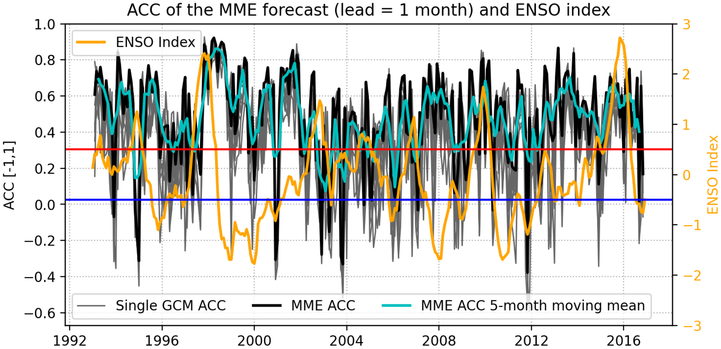
Time series of monthly anomaly correlation coefficient (ACC; left axis, black and grey lines) at one-month lead time from the multi-model ensemble (MME; black) and individual GCMs (grey lines), along with a five-month moving average of MME ACC (cyan line). The orange line shows the monthly ENSO index (Niño 3.4 region, right axis), with red and blue horizontal lines indicating the ±0.5 thresholds for El Niño and La Niña events, respectively.
The seasonal dependency and the influence of different ENSO phases on forecast skill (measured by ACC) are shown in Figure 5. The top-left panel demonstrates forecast skill for the whole period as parameter of comparison. As seen in Figure 3, forecasts initialized during austral winter (JJA) and autumn (MAM) exhibit the highest ACC values, especially at shorter lead times (1–2 months), reaching values as high as 0.68. Conversely, forecasts initialized in austral spring (SON) have notably lower ACC, frequently approaching zero at longer lead times.
Figure 5
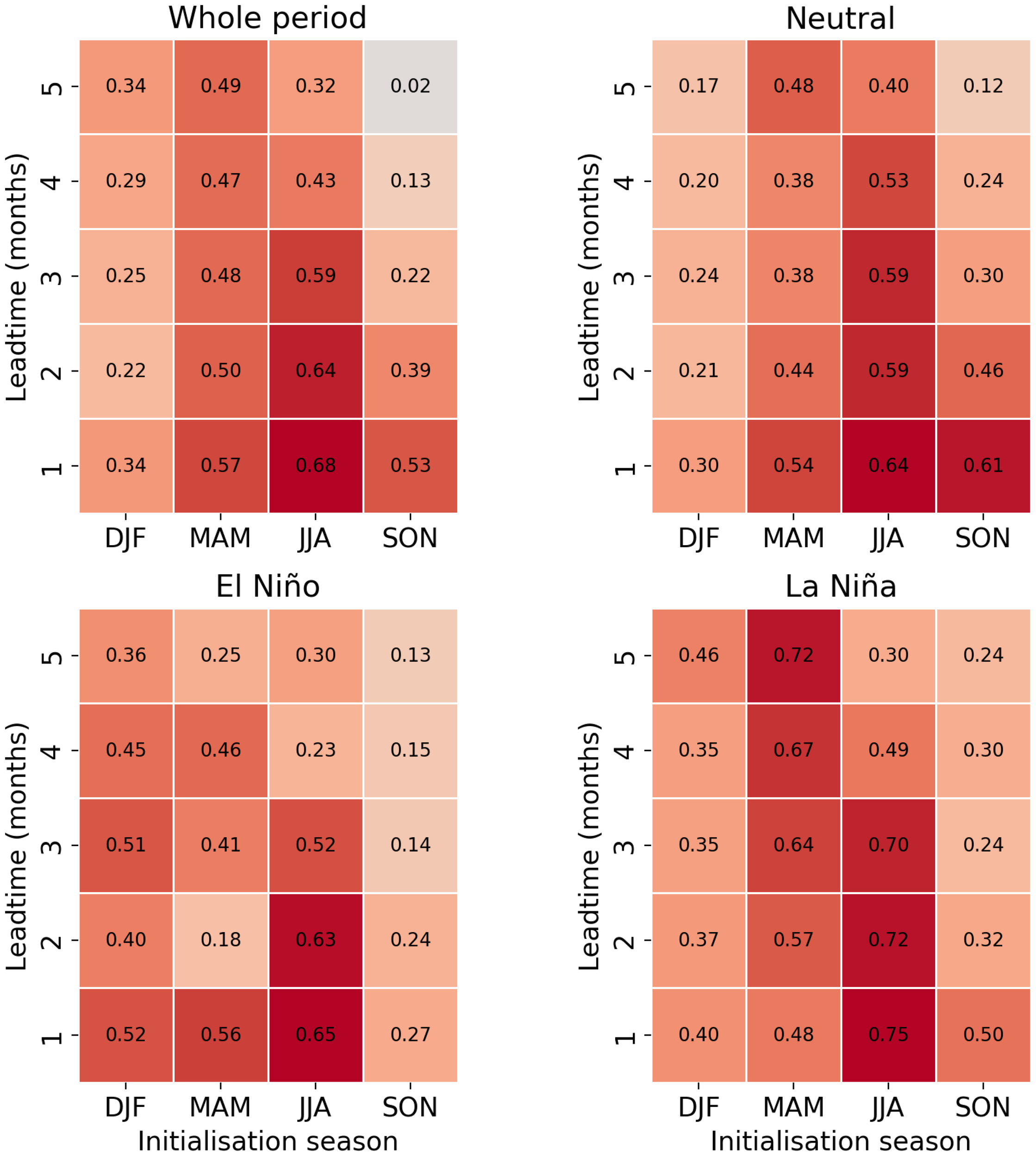
ACC of the Multi-model ensemble (MME) mean per season and ENSO index. El Niño or La Niña events occur with above or below 0.5 threshold, respectively. A neutral phase occurs with ENSO index between ±0.5. The ACC is calculated between anomaly SST from OISST and the MME using three months of data to increase sample size.
When skill is stratified by ENSO phase, distinct patterns emerge. During El Niño conditions, ACC values are enhanced for forecasts initialized in austral summer (DJF), when the ACC reaches values above 0.5 at 1- and 3-month lead times. In contrast, during La Niña conditions, the forecast skill (ACC values) tend to be larger during the austral winter (JJA). The ACC reaches the largest values (0.75) with one-month lead time and 0.70 with three-month lead time in JJA. This reflects a robust influence of La Niña in driving more predictable SST anomalies from winter towards spring. During neutral ENSO conditions, forecast skill is generally diminished in summer and winter but it has the highest ACC values in spring (SON) from one- to three-months lead time.
3.3 Forecast validation against in situ observations
The comparison between satellite-derived SST (OISST) and long-term in situ records provides an important baseline for evaluating the reliability of the MME forecasts at coastal sites. The correlation coefficient between OISST and in situ data from 1993 to 2016 was 0.89 at Leigh and 0.63 at Portobello, values that are consistent with those reported previously by Shears and Bowen (2017) (0.81 and 0.69, respectively). Building on this baseline, we next assess how well the MME forecasts capture SST anomalies compared directly with in situ records.
Time series comparisons between MME forecasts, OISST, and in situ SST anomalies highlight the strengths and limitations of the ensemble forecast at coastal sites (Figure 6). At Leigh, the MME closely tracks observed variability, often reproducing both the peaks and troughs in the observed SST anomalies. This consistency is reflected in high correlations with both OISST (ACC = 0.51) and in situ observations (ACC = 0.53). It is worth noting that despite the high correlation between in situ and satellite data, some large events were not present in both datasets simultaneously. For instance, the large SST anomaly in January 1998 is present in the OISST data but it was not captured by the in situ measurements which showed a large peak in January 1999 instead (Figure 6).
Figure 6
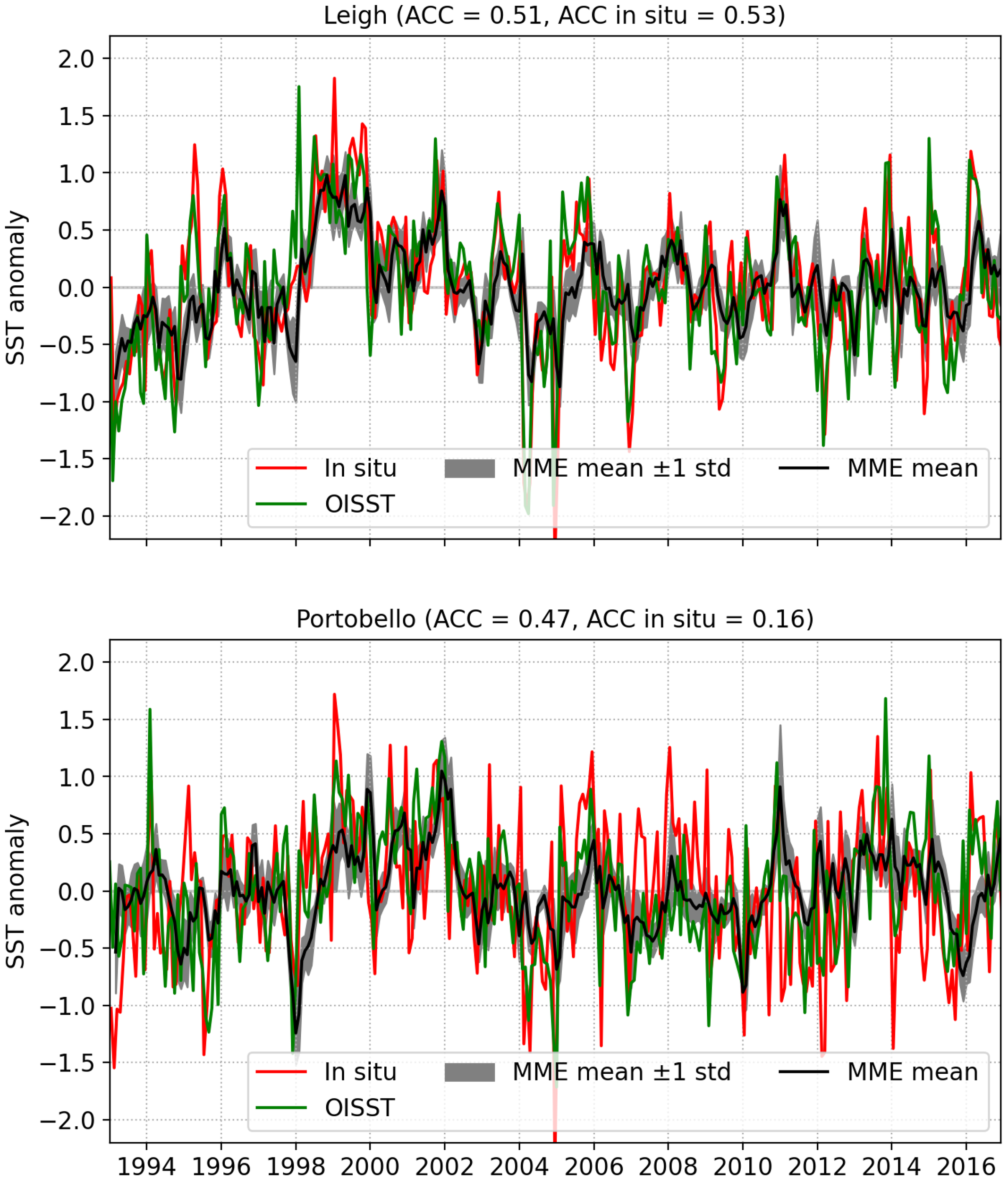
Time series of observed Sea Surface Temperature (SST) anomaly from OISST (green lines), in situ data (red lines) and the MME mean with lead time of one month (black lines) for Leigh and Portobello coastal stations (panels). The grey shade represents MME mean ±1 standard deviation. Each panel title shows the ACC computed between OISST and in situ data with lead time of one month.
At Portobello, the MME agreement with in situ data is much weaker (ACC = 0.16), even though the correlation with OISST is moderate (ACC = 0.47). This discrepancy indicates that while the MME captures regional-scale variability, it does not fully resolve local estuarine dynamics, as expected. The limitation is particularly evident at Otago Harbour, a shallow and narrow estuary with restricted oceanic exchange, where local surface heat fluxes exert strong control on SST variability (Cook et al., 2022).
ACC results per lead time computed between MME forecasts, OISST, and in situ SST anomalies at Leigh and Portobello highlight the contrasting performance between an exposed region and a highly constricted estuarine environment (Figure 7). At Leigh, the MME forecast achieved correlations above 0.5 at one-month lead time against both OISST and in situ data, consistently outperforming the persistences across all lead times. In contrast, forecast skill at Portobello was weaker: ACC values started below 0.5 against OISST and fell below 0.2 against in situ data (bold blue line in Figure 7). Although the MME still outperformed the OISST persistence baseline and produced results comparable to the in situ persistence forecast, the low in situ persistence correlation reflect the large temporal variability evident in Figure 6. The reduction in skill is consistent with the influence of restricted exchange and local heat flux in Otago Harbour, which are not resolved by coarse-resolution GCMs. Overall, these findings demonstrate that the MME is skillful at open-coast sites such as Leigh, but its predictive capacity is reduced in estuarine systems, with Portobello in Otago Harbour illustrating an extreme example of these limitations.
Figure 7

Anomaly correlation coefficient (ACC) comparing the multi-model ensemble (MME, solid lines) and persistence forecasts (dashed lines) against/from OISST (black and red) or in situ data (blue and green). ACC is shown across different lead times (1–5 months) for Leigh and Portobello coastal stations.
3.4 Forecast skill near aquaculture regions
At the selected regions (or grid points) near aquaculture sites, the MME mean captures the variability of the SST anomalies during most of the time analysed, except during large peaks (troughs), such as high (low) SST anomalies in 1998 (2004). As a result, the MME mean exhibits high forecast skill, with ACC values ranging between 0.47 and 0.54 at one-month lead time (Figure 8). Coromandel and Ōpōtiki regions, located in the northeastern area, had the highest ACC values (0.54 and 0.57 respectively), highlighting their stronger link to large-scale and more predictable oceanographic processes. Coromandel has a smaller
Figure 8
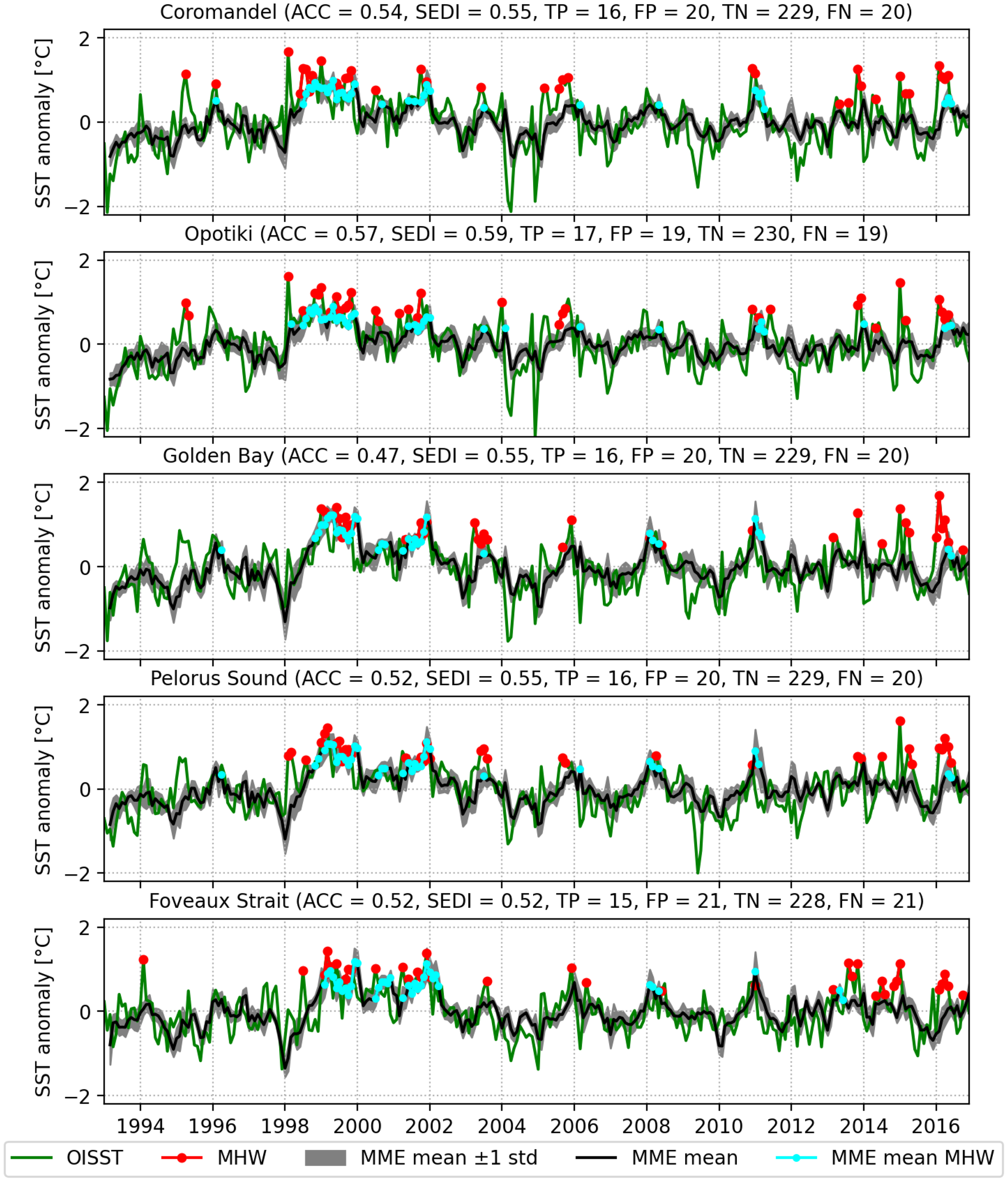
Time series of observed Sea Surface Temperature (SST) anomaly from OISST (green lines) and the MME mean with lead time of one month (black lines) for different aquaculture regions (panels). The red (cyan) dotted lines represent MHW events classified using the OISST (MME). The grey shade represents MME mean ±1 standard deviation. Each panel title shows the ACC computed between OISST and MME mean and SEDI score for MHW events with lead time of one month. The total number of true positive (TP), false positive (FP), true negative (TN), and false negative (FN) are also presented.
ACC compared to Ōpōtiki region, likely due to its location in a more confined area and under riverine influence. Other stations located near straits or influenced by freshwater inputs also exhibited lower ACC values. Golden Bay had the lowest ACC (0.47). This might be associated with its shallow average depth (∼40 m) and river flow influences (Stevens et al., 2021) which makes its SST anomaly more difficult to predict using GCMs which cannot account for these processes due to their coarse spatial resolution. Pelorus Sound and Foveaux Strait, with ACC values of 0.52, indicate skillful forecasts which can be related to the strong connectivity with the nearby ocean (Walters et al., 2001, 2010; Stevens et al., 2021). Despite the moderate to high ACC values, we acknowledge that anomaly SST forecast values may differ from in situ measurements at the actual aquaculture sites, especially if those sites are located in regions with restricted exchange with oceanic waters.
In addition to SST anomalies, the MME also provides skillful predictions of MHW occurrence when compared to observations (Figure 8). The time series show that observed MHW events (red markers) are often reproduced by the deterministic MME forecast (cyan markers), particularly in the late-1990s. Across all sites, the SEDI values (0.52–0.59) indicate that the probabilistic MHW forecasts are substantially better than random chance, with the strongest skill again found in Ōpōtiki. Nevertheless, mismatches still occur, including missed events (false negative) during extreme peaks and false alarms at weaker anomalies (false positive) in the mid-1990s and in 2008. These discrepancies underscore the value of probabilistic forecasts, which convey the likelihood of MHW occurrence and allow users to balance the risks of false alarms against missed events in their decision-making processes (Jacox et al., 2022).
Regional variations in forecast performance are also evident when looking at forecast skill (ACC) at different lead times. For instance, the Ōpōtiki region had relatively high forecast skill even at longer lead times (ACC of about 0.4 at five-month lead) (Figure 9). This is likely due to their exposure to predictable large-scale climate signals such as ENSO. The Coromandel region also has high forecast skill (0.4 ACC) at two-month lead time but it decreases sharply with lead time which might be associated with its shallow location and riverine influence. Golden Bay and Pelorus Sound regions show moderate forecast skill, decreasing more sharply at longer leads, with ACC values below 0.3 at five months. These regions are influenced by more localised coastal processes and they are located near the less predictable position of the South Pacific Subtropical Front which mark the encounter of two distinct water masses (Behrens and Bostock, 2023) and tend to reduce the predictability of SST anomalies. Moreover, Golden Bay has a large seasonal temperature cycle that likely cause monthly SST anomalies to be short-lived, meaning a persistence forecast performs poorly beyond one or two months. Pelorus Sound, by contrast, has a smaller seasonal cycle by being near Cook Strait where ocean mixing dominates reduces temperature intra-annual variability (Stevens, 2014; Stevens et al., 2021). Similarly, Foveaux Strait shows moderate skill at short lead times, declining to around 0.3 by lead time of 5 months (Figure 9).
Figure 9
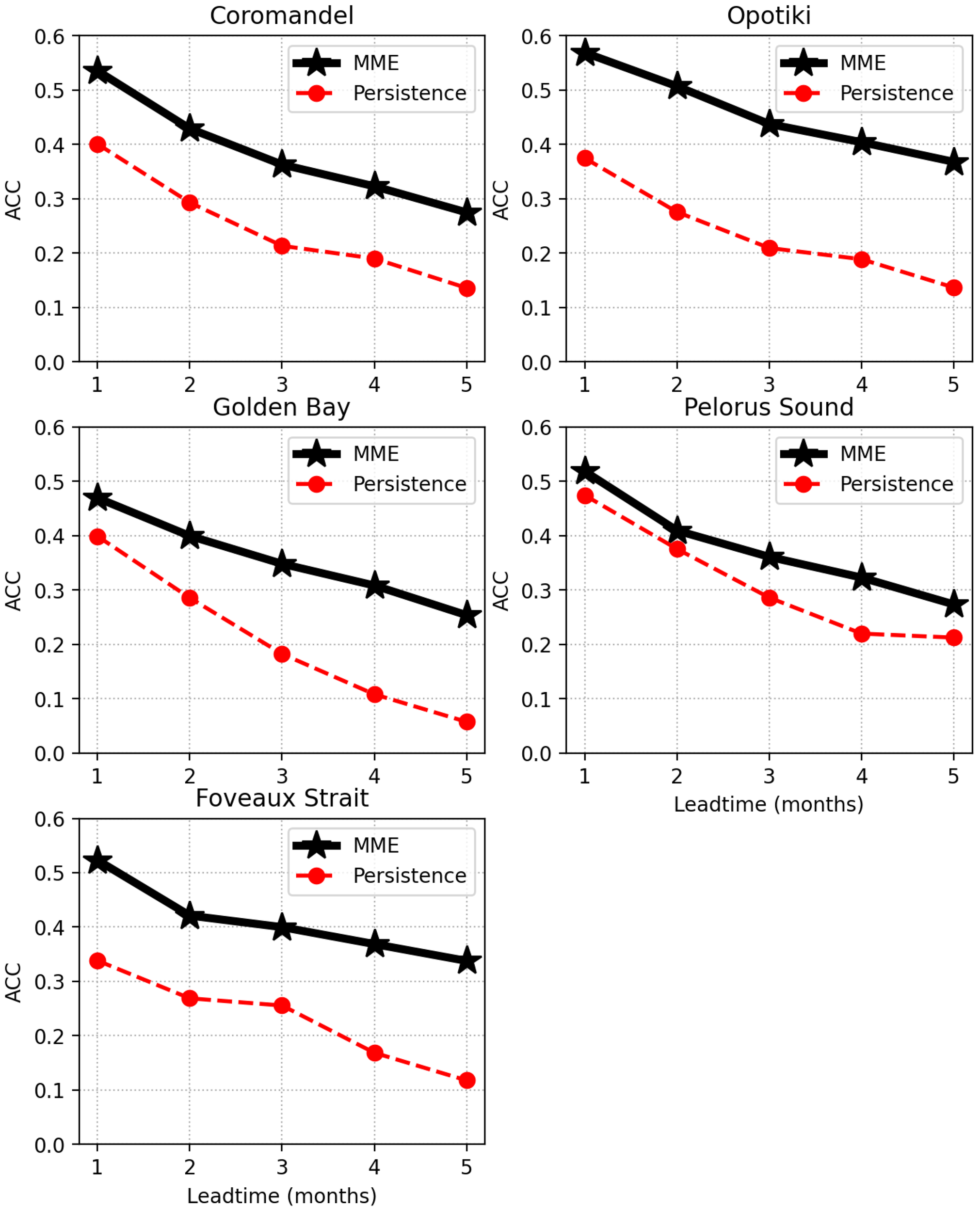
Anomaly correlation coefficient (ACC) comparing the multi-model ensemble (MME, black solid lines) and persistence forecasts (red dashed lines) across different lead times (1–5 months) for key aquaculture regions around Aotearoa New Zealand.
3.5 Marine heatwave probabilistic forecast
We next evaluated the MME’s ability to predict MHWs using a probabilistic framework. An example MHW forecast for the 1997–98 El Niño period illustrates the capabilities of the system (Figure 10). In December 1997, the MME forecast indicated an elevated probability of a MHW developing to the north of Aotearoa New Zealand one month ahead. The observations confirm that a significant warm anomaly occurred, though it was more confined to the northwest of the North Island than forecasted. With a two-month lead (forecast issued in December for February 1998), the MME correctly predicted the encroachment of a MHW along the northeast coast of the North Island. The observed outcome in February 1998 indeed showed MHW conditions along the northeast North Island and even further south along the east coast of the South Island, exceeding the forecasted extent of 0.05 probability (Figure 10). This case demonstrates that the ensemble can capture the general location and timing of MHW events a month or two in advance, even when driven by an unusual strong climate signal (in this case, the 97–98 unusual El Niño). Normally, El Niño (La Niña) phases tend to generate colder (warmer) SST anomalies around Aotearoa New Zealand (de Burgh-Day et al., 2019; Gregory et al., 2024). Nevertheless, the MME was able to accurately predict the occurrence and advance of that MHW event. This was possible via data assimilation which provide accurate model initial conditions and the MME strategy which cancels out model physical errors/biases. Nevertheless, discrepancies in placement and extent, still underline that uncertainty remains in the exact details of the forecast MHW areas.
Figure 10
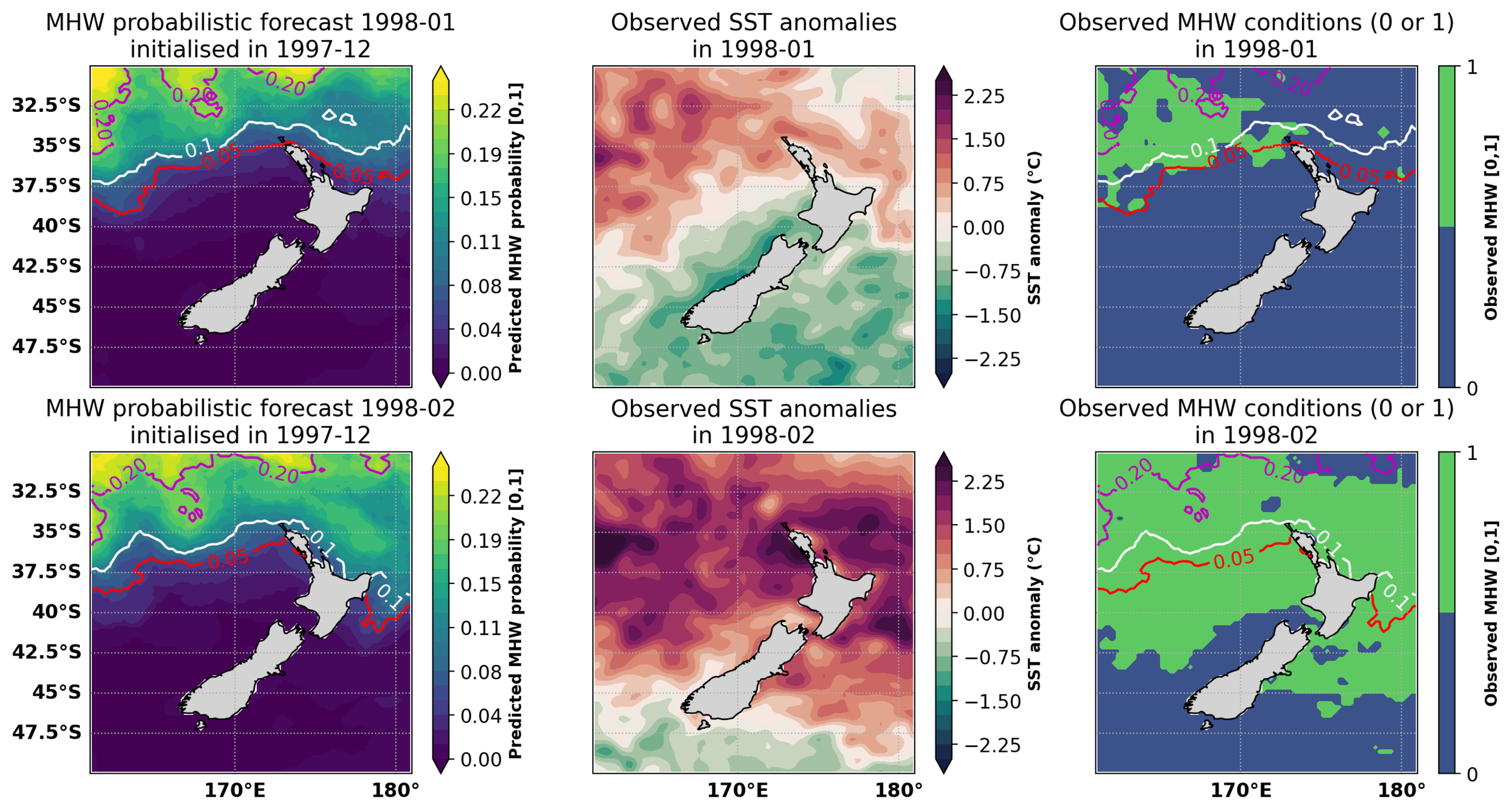
Marine heatwave (MHW) probabilistic forecast (left-hand column), observed Sea Surface Temperature anomalies (central column) and observed MHW (1). The contours of the MHW probabilistic forecast (right-hand column) are shown for January 1998 (top row, lead time = 1 month) and February 1998 (bottom row, lead time = 2 months). The contours in the first and last columns represent 0.2 (20%, purple contour), 0.1 (10%, white contour) and 0.05 (5%, red contour) probability of MHW occurrence.
Across the Aotearoa New Zealand domain, the MME’s probabilistic forecasts show positive SEDI scores at short lead times, indicating better-than-random prediction of MHW occurrence (Figure 11). Skill is highest for lead times of 1–2 months, with SEDI values often in the range of 0.3–0.6 in many regions when using a moderate probability threshold (e.g. 10% chance of MHW) to issue an event forecast. Certain areas, particularly off the northeastern coast and parts of the Tasman Sea west of Aotearoa New Zealand, achieve the highest SEDI, suggesting that MHWs in these locations are tied to more predictable large-scale oceanographic conditions. At longer lead times (4–5 months), SEDI values drop toward zero or even become slightly negative in places, implying little to no skill by 4–5 months lead—a pattern consistent with the loss of SST anomaly correlation over those horizons. Nevertheless, SEDI scores were all above 0.15 near all aquaculture regions for all lead times using a threshold of 0.1 (Table 2).
Figure 11
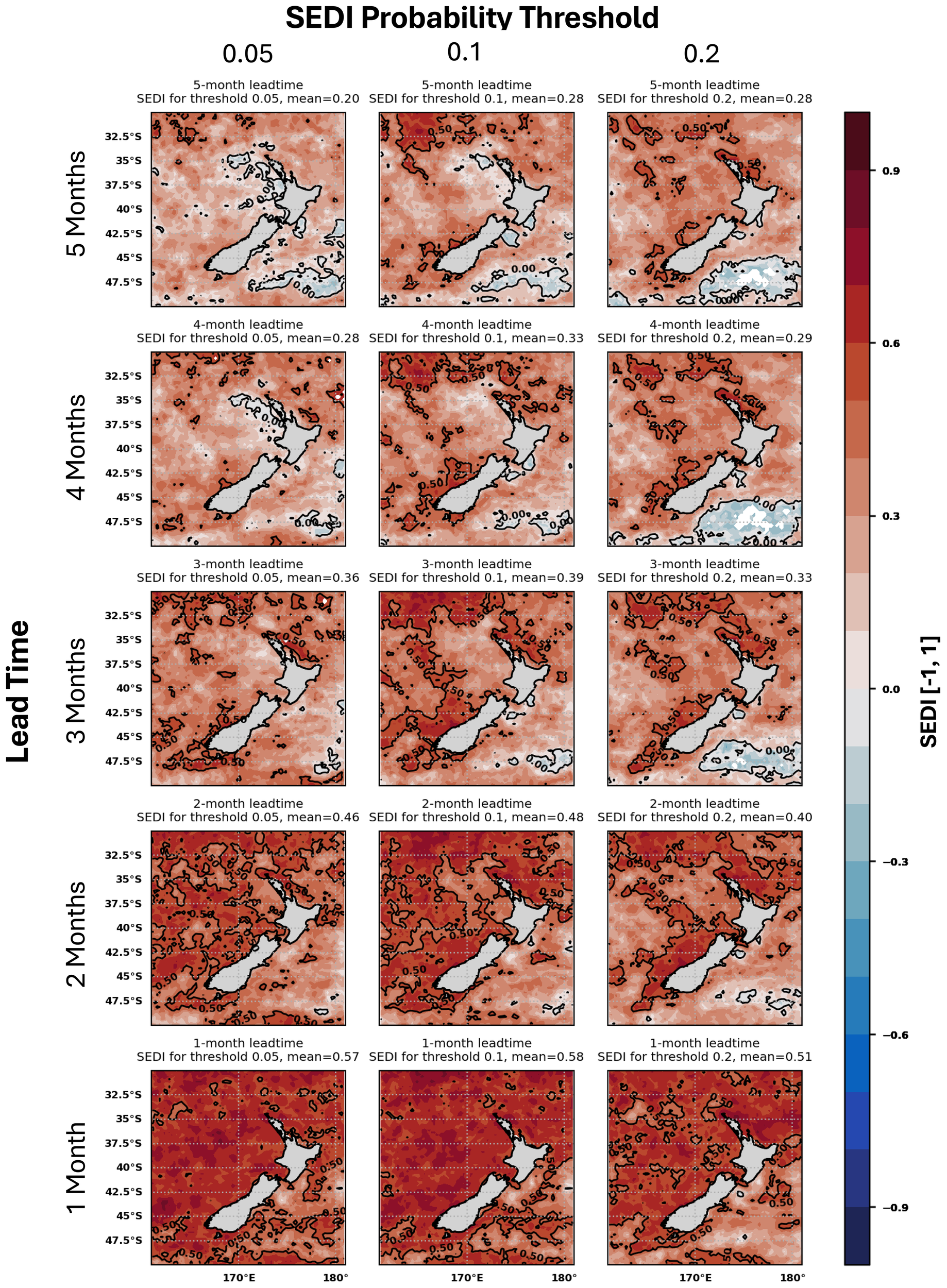
Symmetric External Dependency Index (SEDI) of the marine heatwave (MHW) forecast using probabilistic thresholds of 0.05 (or 5%, left column), 0.1 (or 10%, centre column), and 0.2 (or 20%, right column) to determine occurrence of MHWs. Lead time grows from the bottom row (1 month) to the top row (5-month lead time).
Table 2
| ACC | 1 month | 2 months | 3 months | 4 months | 5 months |
|---|---|---|---|---|---|
| Coromandel | 0.54 | 0.43 | 0.36 | 0.32 | 0.28 |
| Ōpōtiki | 0.57 | 0.51 | 0.44 | 0.40 | 0.37 |
| Golden Bay | 0.47 | 0.40 | 0.35 | 0.31 | 0.25 |
| Pelorus Sound | 0.52 | 0.41 | 0.36 | 0.32 | 0.27 |
| Foveaux Strait | 0.52 | 0.42 | 0.40 | 0.37 | 0.34 |
| RMSE | 1 month | 2 months | 3 months | 4 months | 5 months |
|---|---|---|---|---|---|
| Coromandel | 0.54 | 0.57 | 0.59 | 0.60 | 0.61 |
| Ōpōtiki | 0.49 | 0.51 | 0.53 | 0.54 | 0.55 |
| Golden Bay | 0.54 | 0.56 | 0.57 | 0.58 | 0.60 |
| Pelorus Sound | 0.49 | 0.53 | 0.54 | 0.55 | 0.56 |
| Foveaux Strait | 0.47 | 0.50 | 0.50 | 0.51 | 0.51 |
| SEDI (0.05) | 1 month | 2 months | 3 months | 4 months | 5 months |
|---|---|---|---|---|---|
| Coromandel | 0.51 | 0.37 | 0.07 | 0.06 | 0.08 |
| Ōpōtiki | 0.48 | 0.37 | 0.36 | 0.39 | 0.10 |
| Golden Bay | 0.64 | 0.42 | 0.27 | 0.06 | 0.08 |
| Pelorus Sound | 0.64 | 0.44 | 0.24 | 0.14 | -0.03 |
| Foveaux Strait | 0.49 | 0.28 | 0.46 | 0.28 | 0.15 |
| SEDI (0.1) | 1 month | 2 months | 3 months | 4 months | 5 months |
|---|---|---|---|---|---|
| Coromandel | 0.52 | 0.44 | 0.32 | 0.26 | 0.15 |
| Ōpōtiki | 0.57 | 0.40 | 0.35 | 0.31 | 0.32 |
| Golden Bay | 0.60 | 0.55 | 0.40 | 0.28 | 0.27 |
| Pelorus Sound | 0.65 | 0.44 | 0.35 | 0.33 | 0.23 |
| Foveaux Strait | 0.48 | 0.38 | 0.40 | 0.45 | 0.35 |
| SEDI (0.2) | 1 month | 2 months | 3 months | 4 months | 5 months |
|---|---|---|---|---|---|
| Coromandel | 0.56 | 0.38 | 0.39 | 0.39 | 0.48 |
| Ōpōtiki | 0.53 | 0.48 | 0.51 | 0.45 | 0.52 |
| Golden Bay | 0.51 | 0.52 | 0.36 | 0.47 | 0.40 |
| Pelorus Sound | 0.51 | 0.56 | 0.48 | 0.44 | 0.41 |
| Foveaux Strait | 0.47 | 0.41 | 0.38 | 0.24 | 0.44 |
Multi-model ensemble (MME) SST anomaly forecast skill summary.
Anomaly correlation coeficient (ACC) and root mean square error (RMSE) were calculated between monthly observed and MME SST anomalies using different lead times (months). The probabilistic marine heatwave (MHW) forecast was evaluated against observed MHW (binary) events using the symmetric external dependency index (SEDI) with different probability threshold (0.05, 0.1 and 0.2) for binary re-characterisation. The maximum SEDI score is 1, and scores above (below) zero indicate forecasts that are better (worse) than random chance (Ferro and Stephenson, 2011).
Table 2 summarises the results across the five aquaculture regions. Deterministic metrics (ACC and RMSE) confirm that MME SST anomaly forecasts are most skillful at short lead times (1–2 months). For instance, Ōpōtiki consistently achieve the highest ACC values at 1-month lead time (0.57), while also maintaining relatively low RMSE values, indicating both high correlation and reduced magnitude of errors. Golden Bay and Coromandel exhibit slightly higher RMSE/lower skill overall, possibly reflecting the influence of localised coastal processes not fully resolved at the model’s 0.25° spatial resolution. Pelorus Sound and Foveaux Strait showed intermediate skill probably due their location in straits with increased mixing and less surface heat flux influence. Forecast skill declines progressively with lead time across all regions, with ACC values dropping below 0.38 and RMSE exceeding 0.50 by month 5, highlighting the challenge of accurate seasonal prediction at longer horizons.
Probabilistic MHW forecasts, evaluated using the symmetric extremal dependence index (SEDI), display a similar lead-time dependence, with the highest scores generally occurring for lower probability thresholds (0.05 and 0.1) and shorter lead times, where SEDI values exceed 0.6 for several sites. Conversely, higher thresholds (0.2) maintained high SEDI scores with increasing lead time (Table 2).
A closer examination of the temporal variability of the probabilistic forecasts highlights their ability to signal elevated likelihoods during several observed MHW events across aquaculture sub-regions, though with varying levels of success. For example, between 1998 and 2002 in Coromandel region, the probabilistic forecast frequently issued >20% probability of MHW conditions in the coming month, aligning with several observed MHW occurrences (Figure 12). In contrast, at a more temperate southern region like Foveaux Strait, the MHW forecasts were less confident—probabilities rarely exceeded 20% except during known extreme events—yielding a lower SEDI, though still largely above zero. These region-specific results suggest that forecasting extreme warmth is most effective in regions where MHWs are usually extensions of broad regional anomalies (e.g. north-eastern regions). Conversely, in places where MHWs are shorter and driven by more localised weather fluctuations, the MME forecast system has reduced skill. Nonetheless, even a probabilistic indication of elevated risk (for instance, a forecast of > 10% chance of MHW) can provide aquaculture operations with valuable information prior to extreme heat events.
Figure 12
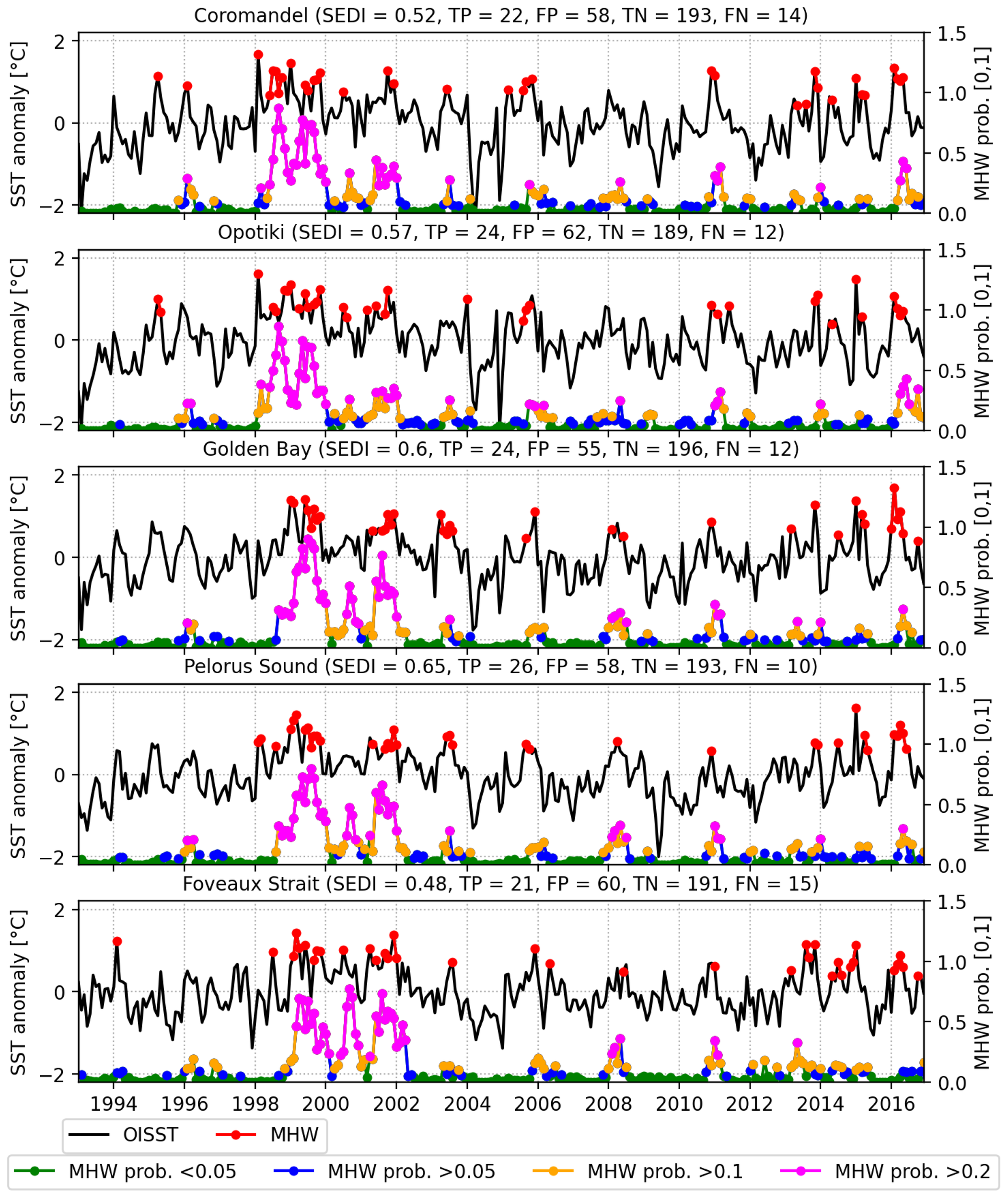
Time series of observed Sea Surface Temperature (SST) anomaly (°C) from OISST (black lines and left-hand y-axis) and observed marine heatwave (MHW) events (red dotted lines) for different aquaculture regions (panels). MHW probabilistic forecast (lead time of one month and right-hand y-axis) are show in different colours. Green, blue, orange, and magenta represent <0.05 (<5%), >0.05 (>5%), >0.1 (>10%), and >0.2 (>20%) probability of MHW (black lines). Each panel title shows the SEDI computed using a probabilistic threshold of 0.1 with one month of forecast lead time and the total number of true positive (TP), false positive (FP), true negative (TN), and false negative (FN) counts.
When compared with the deterministic forecasts shown in Figure 8, the probabilistic approach yields broadly consistent skill using a 0.1 probability threshold (Figure 12). The probabilistic forecast generated a larger (smaller) number of true positive (false negative) compared to the deterministic approach. However, it resulted in a higher number of false positive counts, yielding similar SEDI scores to the deterministic approach. The probabilistic forecasts provide important additional context by clarifying some of the mismatches between observed and deterministic MHW predictions. In several cases where the deterministic forecast either missed an event or produced a false alarm, the probabilistic forecast instead assigned intermediate probabilities (e.g. 5–10%), signalling uncertainty rather than a strict yes/no outcome. Nevertheless, a combined deterministic and probabilistic MHW forecast framework offers both a clear binary signal and gradations of risk, providing a more flexible and practical basis for decision-making in aquaculture and coastal management.
4 Discussion
The results illustrate the advantages of using a multi-model ensemble (MME) approach for predicting sea surface temperature (SST) anomalies and marine heatwave (MHW) occurrences around Aotearoa New Zealand. Consistent with previous research (Hagedorn et al., 2005; Jacox et al., 2022; Fauchereau et al., 2022), the MME demonstrated higher skill (higher ACC and lower RMSE) compared to forecasts from a single GCM and persistence forecasts across most lead times and regions near aquaculture sites. These improvements arise primarily from the ensemble’s ability to reduce systematic biases and uncertainties inherent in individual models (Chaudhari et al., 2013; MacLachlan et al., 2015a).
The MME forecast skill displayed a marked seasonal variability, being notably higher during forecasts initialised between June and August (austral winter) compared to September through December (austral spring and early summer). The reduced skill during the latter period is consistent with previous findings by de Burgh-Day et al. (2022), reflecting decreased ocean-atmosphere coupling and higher atmospheric variability during these months. Importantly, forecast performance was notably linked to the state of the El Niño–Southern Oscillation (ENSO). During La Niña, the forecast skill is improved in winter compared to the whole period analysis. Conversely, during El Niño phases, the forecast increased its performance in summer. During neutral phases, the MME forecast had improved performance during spring months. Results discriminated by seasons and ENSO phases provide more information on the forecast skill compared to a single separation into active ENSO (El Niño and La Niña) vs neutral state shown in Jacox et al. (2022). However, Jacox et al. (2022) focused on analysing the influence of ENSO on the predictability of global MHWs, and a clear understanding of Aotearoa New Zealand’s waters wasn’t their focus.
While Jacox et al. (2022) provided a global assessment of MHW forecast skill, our study offers region-specific insights that extend those findings in meaningful ways for Aotearoa New Zealand. By stratifying forecast skill by ENSO phase and season, we identified distinct “windows of opportunity”, such as austral winter under La Niña conditions and spring under neutral conditions that are directly relevant to aquaculture operations. These seasonal patterns enable stakeholders to adjust confidence in forecasts based on the prevailing climate state, supporting more informed decisions around harvest timing, risk mitigation, and resource allocation. Furthermore, our spatially resolved evaluation across key aquaculture regions reveals variability in skill that is masked in global averages (e.g. Jacox et al., 2022), underscoring the need for localized forecast products (Spillman et al., 2025). These findings demonstrate that the added ensemble size and ENSO-phase breakdown are not merely methodological enhancements, but provide actionable knowledge for coastal management in Aotearoa New Zealand.
Forecast evaluation using in situ data from Leigh and Portobello underscores the resolution-dependent limitations. At Leigh, a station with open connection with the ocean, high correlations between MME, OISST, and in situ data confirm that large-scale signals dominate. However, in Portobello, a station located in the narrow Otago Harbour, the reduced skill demonstrates the importance of fine-scale estuarine dynamics unresolved at coarse model resolution. These results provide a quantitative basis for the resolution caveat noted earlier and suggest that integrating high-resolution regional models would further improve coastal forecast applications.
Spatial variability in forecast skill was significant, with regions influenced by large-scale climate signals (e.g. Ōpōtiki and Coromandel) showing higher skill compared to those dominated by local processes, such as freshwater inflows or coastal currents (e.g. Golden Bay, Pelorus Sound, Foveaux Strait). The higher predictability at regions like Ōpōtiki aligns well with previous studies that emphasize the role of ENSO-driven SST variability in the western and northeastern regions of Aotearoa New Zealand (de Burgh-Day et al., 2019). In contrast, lower predictability in areas such as Golden Bay could be attributed to shallow waters, river discharge, and strong seasonal temperature cycles (Stevens et al., 2022), factors typically challenging for coupled climate models to accurately represent. This suggests the need for application of downscaled physical simulations to more accurately predict these coastal processes (e.g. Santana et al., 2023, 2025). Operational use of MME forecasts should be preceded by validation against in situ data, especially in regions with limited oceanic exchange.
It is worth noting that SST anomalies analysed in this study are monthly averaged, whereas daily variability can generate higher temperature extremes that may be more impactful for marine organisms and aquaculture operations. While our use of monthly SST averages enables consistent evaluation across models and lead times, it inherently limits the detection of short-duration marine heatwave events. These transient but ecologically significant events may be missed in our framework, and future work should explore higher-frequency forecasts or downscaled regional models to address this gap. This also highlights the importance of having regional high-frequency ocean forecasts for more accurate predictions (Spillman et al., 2025).
Marine heatwave forecasts evaluated using the Symmetric Extremal Dependence Index (SEDI) indicate that the MME has significant predictive skill, especially at shorter lead times (1–2 months), consistent with global assessments of marine heatwave predictability (Jacox et al., 2022). On average, however, the skill declines beyond three months (SEDI < 0.4). Spatially, higher SEDI values were found around the northern and northeastern coasts, affirming these regions’ responsiveness to predictable ENSO-related SST anomalies (de Burgh-Day et al., 2019). Moreover, SEDI scores were all positive (better-than-random prediction) near all aquaculture regions for all lead times using a threshold greater than 0.1. These results emphasise the value of probabilistic forecasts, at moderate confidence predictions (10% threshold) can inform proactive management decisions in aquaculture sectors facing elevated thermal stress risk (Smith et al., 2021; Cook et al., 2024).
5 Conclusion
This study assessed the predictive skill of a multi-model ensemble (MME) for seasonal forecasting of sea surface temperatures (SST) anomalies and marine heatwave (MHW) events around Aotearoa New Zealand. The MME consistently outperformed individual models and persistence forecasts, emphasising the benefit of combining multiple general circulation models (GCMs) to improve forecast reliability. Forecast skill exhibited clear seasonal and spatial variability, with the highest accuracy found during winter initialisations and in northern regions more influenced by predictable climate drivers, notably ENSO.
For regional aquaculture management, the MME offers substantial value, particularly at one- and two-month lead times, enabling early-warning strategies and proactive mitigation of MHW impacts. However, the decline in forecast skill at longer lead times, lack of coastal processes (e.g. tides and riverine input), and model coarse spatial resolution highlight the continuing challenges faced by seasonal forecasting systems. Future work should further explore the integration of regional downscaling approaches and more detailed physical-biological coupled models to enhance the prediction of aquaculture productivity directly linked to SST variability.
Statements
Data availability statement
The MME outputs are available on https://cds.climate.copernicus.eu/datasets/seasonal-monthly-ocean?tab=download and are accessible via an API (Application Programmer Interface, see https://github.com/ecmwf/cdsapi) which allows the user to select variables of interest, initial month, lead-time (in months), and download the resulting files in grib or netcdf – data formats both widely used in the meteorological and climate communities. More details can be found within the CDS documentation, at https://confluence.ecmwf.int/display/CKB/C3S+Seasonal+Forecasts (last accessed on 25th of June 2024). Code used for the analysis in this study can be found at https://github.com/nicolasfauchereau/SST_forecasting/blob/main/notebooks/.
Author contributions
RS: Formal Analysis, Investigation, Methodology, Validation, Visualization, Writing – original draft, Writing – review & editing. NR: Writing – review & editing, Investigation. NF: Conceptualization, Data curation, Investigation, Methodology, Software, Validation, Visualization, Writing – review & editing. HL: Investigation, Writing – review & editing. FT: Writing – review & editing. PG: Writing – review & editing. NB: Writing – review & editing.
Funding
The author(s) declare financial support was received for the research and/or publication of this article. This research has been undertaken through the National Institute for Water and Atmospheric Research Ltd’s Coasts & Estuaries National Centre (project CENC2501 and its predecessors), and it was funded through Strategic Science Investment Funding from the Ministry for Business, Innovation and Employment (MBIE, contract C01X1703), and support from MBIE Endeavour Fund Tau Ki Ākau (contract UOWX2206).
Acknowledgments
We thank the different Institutions that made their model simulations available for validation and analysis, Copernicus Climate Data Store for hosting this large dataset, and NOAA for providing calibrated sea surface temperature observations.
Conflict of interest
Authors RS, NR, NF, HL, PG, and NB were employed by the company Earth Sciences New Zealand.
The remaining author declares that the research was conducted in the absence of any commercial or financial relationships that could be construed as a potential conflict of interest.
Generative AI statement
The author(s) declare that Generative AI was used in the creation of this manuscript. ChatGPT was used to refine the grammar and fluidity in the manuscript.
Any alternative text (alt text) provided alongside figures in this article has been generated by Frontiers with the support of artificial intelligence and reasonable efforts have been made to ensure accuracy, including review by the authors wherever possible. If you identify any issues, please contact us.
Publisher’s note
All claims expressed in this article are solely those of the authors and do not necessarily represent those of their affiliated organizations, or those of the publisher, the editors and the reviewers. Any product that may be evaluated in this article, or claim that may be made by its manufacturer, is not guaranteed or endorsed by the publisher.
References
1
Behrens E. Bostock H. (2023). The response of the subtropical front to changes in the southern hemisphere westerly winds—evidence from models and observations. J. Geophysical Research: Oceans128, e2022JC019139. doi: 10.1029/2022JC019139
2
Behrens E. Rickard G. Rosier S. Williams J. Morgenstern O. Stone D. (2022). Projections of future marine heatwaves for the oceans around New Zealand using New Zealand’s earth system model. Front. Climate4, 798287. doi: 10.3389/fclim.2022.798287
3
Bi D. Dix M. Marsland S. O’Farrell S. Rashid H. Uotila P. et al . (2013). The ACCESS coupled model: description, control climate and evaluation. Aust. Meteorological Oceanographic J.63, 41–64. doi: 10.22499/2.6301.004
4
Broekhuizen N. Plew D. R. Pinkerton M. H. Gall M. G. (2021). Sea temperature rise over the period 2002–2020 in Pelorus Sound, New Zealand–with possible implications for the aquaculture industry. New Z. J. Mar. Freshw. Res.55, 46–64. doi: 10.1080/00288330.2020.1868539
5
Chaudhari H. S. Pokhrel S. Mohanty S. Saha S. K. (2013). Seasonal prediction of Indian summer monsoon in ncep coupled and uncoupled model. Theor. Appl. climatology114, 459–477. doi: 10.1007/s00704-013-0854-8
6
Cheng M. C. Ericson J. A. Ragg N. L. Dunphy B. J. Zamora L. N. (2025). Mussels, perna canaliculus, as biosensors for climate change: concurrent monitoring of heart rate, oxygen consumption and gaping behaviour under heat stress. New Z. J. Mar. Freshw. Res.59, 1621–1639. doi: 10.1080/00288330.2025.2461757
7
Chiswell S. Grant B. (2018). New Zealand coastal sea surface temperature. Prepared for the Ministry for the Environment. Tech. Rep. Available online at: https://environment.govt.nz/assets/Publications/Files/nz-coastal-sea-surface-temperature.PDF (Accessed November 5, 2025).
8
Cook K. M. Dunn M. R. Behrens E. Pinkerton M. H. Law C. S. Cummings V. J. (2024). The impacts of marine heatwaves on ecosystems and fisheries in aotearoa New Zealand. New Z. J. Mar. Freshw. Res.59, 1530–1560. doi: 10.1080/00288330.2024.2436661
9
Cook F. Smith R. O. Roughan M. Cullen N. J. Shears N. Bowen M. (2022). Marine heatwaves in shallow coastal ecosystems are coupled with the atmosphere: Insights from half a century of daily in situ temperature records. Front. Climate4, 1012022. doi: 10.3389/fclim.2022.1012022
10
Cornelissen L. Behrens E. Fernandez D. Sutton P. J. (2025). Increased stratification intensifies surface marine heatwaves north-east of Aotearoa New Zealand in New Zealand’s Earth System model. J. South. Hemisphere Earth Syst. Sci.75. doi: 10.1071/ES23030
11
de Burgh-Day C. O. Spillman C. M. Smith G. Stevens C. L. (2022). Forecasting extreme marine heat events in key aquaculture regions around New Zealand. J. South. Hemisphere Earth Syst. Sci.72, 58–72. doi: 10.1071/ES21012
12
de Burgh-Day C. O. Spillman C. M. Stevens C. Alves O. Rickard G. (2019). Predicting seasonal ocean variability around New Zealand using a coupled ocean-atmosphere model. New Z. J. Mar. Freshw. Res.53, 201–221. doi: 10.1080/00288330.2018.1538052
13
Deutscher Wetterdienst (2020). German climate forecast system gcfs2.1.
14
Fauchereau N. Ramsay D. Noll B. Lorrey A. (2022). Open data and open source software for the development and validation of multi-model monthly-to-seasonal probabilistic forecasts for the Pacific Islands. Authorea Preprints. doi: 10.1002/essoar.10511702.1
15
Ferro C. A. Stephenson D. B. (2011). Extremal dependence indices: improved verification measures for deterministic forecasts of rare binary events. Weather Forecasting26, 699–713. doi: 10.1175/WAF-D-10-05030.1
16
Gregory C. H. Holbrook N. J. Marshall A. G. Spillman C. M. (2024). Sub-seasonal to seasonal drivers of regional marine heatwaves around Australia. Climate Dynamics62, 6599–6623. doi: 10.1007/s00382-024-07226-x
17
Hagedorn R. Doblas-Reyes F. J. Palmer T. N. (2005). The rationale behind the success of multi-model ensembles in seasonal forecasting – I. Basic concept. Tellus A: Dynamic Meteorology Oceanography57, 219–233. doi: 10.1111/j.1600-0870.2005.00103.x
18
Hirahara S. Kubo Y. Yoshida T. Komori T. Chiba J. Takakura T. et al . (2023). Japan meteorological agency/meteorological research institute coupled prediction system version 3 (jma/mri–cps3). J. Meteorological Soc. Japan101, 149–169. doi: 10.2151/jmsj.2023-009
19
Hobday A. J. Alexander L. V. Perkins S. E. Smale D. A. Straub S. C. Oliver E. C. et al . (2016). A hierarchical approach to defining marine heatwaves. Prog. oceanography141, 227–238. doi: 10.1016/j.pocean.2015.12.014
20
Hobeichi S. Abramowitz G. Sen Gupta A. Taschetto A. S. Richardson D. Rampal N. et al . (2024). How well do climate modes explain precipitation variability? Climate Atmospheric Sci.7, 1–9. doi: 10.1038/s41612-024-00853-5
21
Holbrook N. J. Scannell H. A. Sen Gupta A. Benthuysen J. A. Feng M. Oliver E. C. et al . (2019). A global assessment of marine heatwaves and their drivers. Nat. Commun.10, 2624. doi: 10.1038/s41467-019-10206-z
22
Huang B. Liu C. Banzon V. Freeman E. Graham G. Hankins B. et al . (2021). Improvements of the daily optimum interpolation sea surface temperature (DOISST) version 2.1. J. Climate34, 2923–2939. doi: 10.1175/JCLI-D-20-0166.1
23
Jacox M. G. Alexander M. A. Amaya D. Becker E. Bograd S. J. Brodie S. et al . (2022). Global seasonal forecasts of marine heatwaves. Nature604, 486–490. doi: 10.1038/s41586-022-04573-9
24
Johnson S. J. Stockdale T. N. Ferranti L. Balmaseda M. A. Molteni F. Magnusson L. et al . (2019). SEAS5: the new ECMWF seasonal forecast system. Geoscientific Model. Dev.12, 1087–1117. doi: 10.5194/gmd-12-1087-2019
25
Lin H. (2020). GEM-NEMO global coupled model for seasonal predictions (World Climate Research Programme).
26
Lin H. Merryfield W. J. Muncaster R. Smith G. C. Markovic M. Dupont F. et al . (2020). The canadian seasonal to interannual prediction system version 2 (cansipsv2). Weather Forecasting35, 1317–1343. doi: 10.1175/WAF-D-19-0259.1
27
Lledó L. Cionni I. Torralba V. Bretonniere P.-A. Samso M. (2020). Seasonal prediction of euro-atlantic teleconnections from multiple systems. Environ. Res. Lett.15, 074009. doi: 10.1088/1748-9326/ab87d2
28
MacLachlan C. Arribas A. Peterson K. A. Maidens A. Fereday D. Scaife A. et al . (2015a). Global seasonal forecast system version 5 (glosea5): A high-resolution seasonal forecast system. Q. J. R. Meteorological Soc.141, 1072–1084. doi: 10.1002/qj.2396
29
MacLachlan C. Arribas A. Peterson K. A. Maidens A. Fereday D. Scaife A. A. et al . (2015b). Description of glosea5: the met office high resolution seasonal forecast system. Q. J. R. Meteorological Soc. doi: 10.1002/qj.2396
30
Ministry for Primary Industries (2023). Aquaculture Strategy: 2023 Implementation Plan ( The New Zealand Government).
31
Montie S. Thoral F. Smith R. O. Cook F. Tait L. W. Pinkerton M. H. et al . (2024). Seasonal trends in marine heatwaves highlight vulnerable coastal ecoregions and historic change points in New Zealand. New Z. J. Mar. Freshw. Res.58, 274–299. doi: 10.1080/00288330.2023.2218102
32
Oliver E. C. Burrows M. T. Donat M. G. Sen Gupta A. Alexander L. V. Perkins-Kirkpatrick S. E. et al . (2019). Projected marine heatwaves in the 21st century and the potential for ecological impact. Front. Mar. Sci.6, 734. doi: 10.3389/fmars.2019.00734
33
Oliver E. C. Donat M. G. Burrows M. T. Moore P. J. Smale D. A. Alexander L. V. et al . (2018). Longer and more frequent marine heatwaves over the past century. Nat. Commun.9, 1324. doi: 10.1038/s41467-018-03732-9
34
Patterson M. Befort D. J. Lockwood J. F. Slattery J. Weisheimer A. (2025). The representation of surface temperature trends in c3s seasonal forecast systems. Atmospheric Sci. Lett.26. doi: 10.1002/asl.1316
35
Primavera J. H. (2006). Overcoming the impacts of aquaculture on the coastal zone. Ocean Coast. Manage.49, 531–545. doi: 10.1016/j.ocecoaman.2006.06.018
36
Rampal N. Broekhuizen N. Plew D. Zeldis J. Noll B. Meyers T. et al . (2023). Seasonal forecasting of mussel aquaculture meat yield in the Pelorus Sound. Front. Mar. Sci.10, 1195921. doi: 10.3389/fmars.2023.1195921
37
Saha S. Moorthi S. Wu X. Wang J. Nadiga S. Tripp P. et al . (2014). The ncep climate forecast system version 2. J. Climate27, 2185–2208. doi: 10.1175/JCLI-D-12-00823.1
38
Sanna A. Borrelli A. Athanasiadis P. Materia S. Storto A. Navarra A. et al . (2017). CMCC-SPS3: The CMCC Seasonal Prediction System 3 ( Tech. rep., Centro Euro-Mediterraneo sui Cambiamenti Climatici).
39
Santana R. Costa F. B. Mignac D. Santana A. N. Vidal V. F. d. S. et al . (2020). Model sensitivity experiments on data assimilation, downscaling and tides for the representation of the cape são tomé eddies. Ocean Dynamics70, 77–94. doi: 10.1007/s10236-019-01307-w
40
Santana R. Macdonald H. O’Callaghan J. Powell B. Wakes S. Suanda S. (2023). Data assimilation sensitivity experiments in the east auckland current system using 4d-var. Geoscientific Model. Dev.16, 3675–3698. doi: 10.5194/gmd-16-3675-2023
41
Santana R. O’Callaghan J. Macdonald H. Suanda S. H. Wakes S. (2025). Eddy-driven cross-shelf exchange and variability in the east auckland current. J. Geophysical Research: Oceans130, e2024JC021601. doi: 10.1029/2024JC021601
42
Santana R. Suanda S. H. Macdonald H. O’Callaghan J. (2021). Mesoscale and wind-driven intra-annual variability in the east auckland current. Sci. Rep.11, 9764. doi: 10.1038/s41598-021-89222-3
43
Shears N. T. Bowen M. M. (2017). Half a century of coastal temperature records reveal complex warming trends in western boundary currents. Sci. Rep.7, 14527. doi: 10.1038/s41598-017-14944-2
44
Smale D. A. Wernberg T. Oliver E. C. Thomsen M. Harvey B. P. Straub S. C. et al . (2019). Marine heatwaves threaten global biodiversity and the provision of ecosystem services. Nat. Climate Change9, 306–312. doi: 10.1038/s41558-019-0412-1
45
Smith K. E. Burrows M. T. Hobday A. J. Sen Gupta A. Moore P. J. Thomsen M. et al . (2021). Socioeconomic impacts of marine heatwaves: Global issues and opportunities. Science374, eabj3593. doi: 10.1126/science.abj3593
46
Smith K. E. Gupta A. S. Amaya D. Benthuysen J. A. Burrows M. T. Capotondi A. et al . (2025). Baseline matters: Challenges and implications of different marine heatwave baselines. Prog. Oceanography231, 103404. doi: 10.1016/j.pocean.2024.103404
47
Spillman C. M. Hobday A. J. Behrens E. Feng M. Capotondi A. Cravatte S. et al . (2025). What makes a marine heatwave forecast useable, useful and used? Prog. Oceanography234, 103464. doi: 10.1016/j.pocean.2025.103464
48
Stevens C. (2014). Residual flows in cook strait, a large tidally dominated strait. J. Phys. Oceanography44, 1654–1670. doi: 10.1175/JPO-D-13-041.1
49
Stevens C. L. O’Callaghan J. M. Chiswell S. M. Hadfield M. G. (2021). Physical oceanography of New Zealand/Aotearoa shelf seas–a review. New Z. J. Mar. Freshw. Res.55, 6–45. doi: 10.1080/00288330.2019.1588746
50
Stevens C. L. Spillman C. M. Behrens E. Broekhuizen N. Holland P. Matthews Y. et al . (2022). Horizon scan on the benefits of ocean seasonal forecasting in a future of increasing marine heatwaves for Aotearoa New Zealand. Front. Climate4, 907919. doi: 10.3389/fclim.2022.907919
51
Thoral F. Montie S. Thomsen M. S. Tait L. W. Pinkerton M. H. Schiel D. R. (2022). Unravelling seasonal trends in coastal marine heatwave metrics across global biogeographical realms. Sci. Rep.12, 7740. doi: 10.1038/s41598-022-11908-z
52
Thornton H. Smith D. Scaife A. Dunstone N. (2023). Seasonal predictability of the east atlantic pattern in late autumn and early winter. Geophysical Res. Lett.50, e2022GL100712. doi: 10.1029/2022GL100712
53
Walters R. A. Gillibrand P. A. Bell R. G. Lane E. M. (2010). A study of tides and currents in Cook Strait, New Zealand. Ocean dynamics60, 1559–1580. doi: 10.1007/s10236-010-0353-8
54
Walters R. A. Goring D. G. Bell R. G. (2001). Ocean tides around New Zealand. New Z. J. Mar. Freshw. Res.35, 567–579. doi: 10.1080/00288330.2001.9517023
55
Wedd R. Alves O. de Burgh-Day C. Down C. Griffiths M. Hendon H. H. et al . (2022). ACCESS-S2: the upgraded Bureau of Meteorology multi-week to seasonal prediction system. J. South. Hemisphere Earth Syst. Sci.72, 218–242. doi: 10.1071/ES22026
56
Zeldis J. Hadfield M. Booker D. (2013). Influence of climate on pelorus sound mussel aquaculture yields: predictive models and underlying mechanisms. Aquaculture Environ. Interact.4, 1–15. doi: 10.3354/aei00066
Summary
Keywords
ensemble forecast, coupled models, aquaculture, El Niño-Southern oscillation, marine heatwave
Citation
Santana R, Rampal N, Fauchereau N, Lewis H, Thoral F, Gibson PB and Broekhuizen N (2025) Multi-model ensemble forecasts of sea surface temperatures and marine heatwaves for Aotearoa New Zealand. Front. Mar. Sci. 12:1607806. doi: 10.3389/fmars.2025.1607806
Received
08 April 2025
Accepted
27 October 2025
Published
14 November 2025
Volume
12 - 2025
Edited by
Toru Miyama, Japan Agency for Marine-Earth Science and Technology, Japan
Reviewed by
Carlos Calvo-Sancho, University of Valladolid, Spain
Yiwen Li, China University of Geosciences (Beijing) Energy Institute, China
Updates
Copyright
© 2025 Santana, Rampal, Fauchereau, Lewis, Thoral, Gibson and Broekhuizen.
This is an open-access article distributed under the terms of the Creative Commons Attribution License (CC BY). The use, distribution or reproduction in other forums is permitted, provided the original author(s) and the copyright owner(s) are credited and that the original publication in this journal is cited, in accordance with accepted academic practice. No use, distribution or reproduction is permitted which does not comply with these terms.
*Correspondence: Rafael Santana, rafael.santana@niwa.co.nz
Disclaimer
All claims expressed in this article are solely those of the authors and do not necessarily represent those of their affiliated organizations, or those of the publisher, the editors and the reviewers. Any product that may be evaluated in this article or claim that may be made by its manufacturer is not guaranteed or endorsed by the publisher.