Spatiotemporal impact of mesoscale eddies on chlorophyll-a concentration in the North Atlantic

Introduction: Mesoscale eddies play a crucial role in energy transport and ecological regulation in the North Atlantic Ocean.

Methods: Based on multi-source datasets, including satellite remote sensing and Argo float observations from 2009 to 2018, this study employs the Velocity Gradient Detection (VGD) method to identify eddy boundaries and cores, in combination with a spatiotemporal dynamic matching technique, to systematically analyze eddy characteristics and their impacts on chlorophyll-a (Chl-a) concentrations.

Results: Results show that eddy activity is predominantly concentrated in the Gulf Stream extension region (24°N–48°N, 40°W–60°W). Cyclonic eddies significantly elevate surface Chl-a concentrations (0.6–1.8 mg/m³) through upwelling processes, while anticyclonic eddies induce localized enrichment (15%–25% increase) along their peripheries, exhibiting marked seasonal variability. Vertical analysis reveals that eddy-induced Chl-a anomalies can peak at depths of 50–70 m, effectively enhancing subsurface primary productivity. Overall, eddy-driven Chl-a variations contribute approximately 20% to regional primary production.

Discussion: These findings highlight the functional importance of mesoscale eddies in regulating phytoplankton biomass and underscore their role in advancing our understanding of the marine carbon cycle under changing climate conditions.

1 Introduction

Marine ecosystems are a crucial component of the Earth’s climate system, closely linked to the global carbon cycle through their biogeochemical cycles. Chlorophyll-a (Chl-a) concentration, as a key indicator, reflects the spatial and temporal distribution patterns of ocean primary productivity (Lévy et al., 2018; Sukhonos and Alexander, 2022).

The North Atlantic, as a critical region in the global marine ecosystem, exhibits unique Chl-a distribution patterns. These patterns are largely shaped by its complex circulation system, the prevalence of mesoscale eddy activities, and pronounced seasonal variability (Fu and Morrow, 2013; Chen et al., 2022; Mikaelyan et al., 2023). Mesoscale eddies, as dynamic features of ocean circulation, significantly influence the availability and transport of nutrients through vertical upwelling and horizontal advection. These processes inject nutrients such as nitrate and phosphate into the euphotic zone, enhancing the growth of phytoplankton.

Chl-a, as a photosynthetic pigment in phytoplankton, serves as a core assessment index for driving material and energy cycles in marine ecosystems (Tang and Chen, 2016; Browning et al., 2021). Its concentration distribution not only reflects the spatial patterns of phytoplankton biomass (McGillicuddy et al., 2007; Zhang et al., 2019; Han et al., 2024) but also enables the quantitative estimation of regional carbon fixation capacity (Sundararaman and Shanmugam, 2023).

In recent years, many scholars have conducted in-depth studies on the chlorophyll distribution in the North Atlantic using remote sensing data, Argo data, and field measurements (George et al., 2021). The results indicate that chlorophyll distribution is closely related to latitude, with higher concentrations in high-latitude areas and lower concentrations in tropical regions. Additionally, statistical analysis using Argo data shows that the northern region (47°N-54°N) reaches its peak in mid-May (17 mmol m^-3 d^-1), while the southern region exhibits higher NPP in winter and lower NPP in summer (with a peak of about 10 mmol m^-3 d^-1), demonstrating distinct regional and seasonal variations (Wang and Liu, 2024).

Mesoscale eddies, as an important component of the oceanic dynamic system, alter nutrient distribution and light conditions in the region (Androulidakis et al., 2020; Keppler et al., 2024), thus affecting the distribution and concentration of chlorophyll (Villas Bôas et al., 2015; Sathyendranath et al., 2017).

Research shows that mesoscale eddies influence chlorophyll distribution through eddy stirring, with anticyclonic eddies causing higher chlorophyll anomalies than cyclonic eddies (Follows and Dutkiewicz, 2001), potentially linked to additional mechanisms like Ekman pumping or mixing. In winter, chlorophyll anomalies show a positive correlation with mixed layer depth, but the relationship is not significant in other seasons. The influence of eddies varies by region and eddy type at different latitudes, either enhancing or suppressing chlorophyll distribution and concentration (Gaube et al., 2014). In the mid-latitude regions, studies have found that chlorophyll anomalies are inversely related to mixed layer depth, indicating that eddies affect phytoplankton growth by altering vertical structure (He et al., 2019). Anticyclonic eddies lower isopycnal surfaces, while cyclonic eddies elevate them, influencing nutrient upwelling and chlorophyll concentration. In specific areas like the Canary Islands, cyclonic eddies enhance chlorophyll concentration and distribution by nutrient pumping and vertical uplift of deep chlorophyll maxima, transporting high-chlorophyll waters downstream (Uchiyama et al., 2017; Drouin et al., 2022). In the Sargasso Sea’s mode water eddies, even anticyclonic eddies can provide nutrients through upwelling and mixing, maintaining a strong deep chlorophyll layer (Smith et al., 1996). Overall, the effect of mesoscale eddies on chlorophyll distribution in the North Atlantic is complex, dependent on region, eddy type, and specific mechanisms.

This study focuses on the North Atlantic, integrating satellite observation data (such as altimeter data, sea surface temperature, Chl-a concentration, and sea surface wind fields) with historical field observation data (such as Argo buoys and shipboard CTD profiles). We construct a high-resolution mesoscale eddy dataset covering the North Atlantic, including eddy trajectories, propagation distances and speeds, radii, lifecycles, vertical temperature-salinity structures, and accompanying Chl-a distribution characteristics. The study aims to explore the interdecadal variation trends in eddy activity strength, lifecycle, and ecological effects, and assess the potential evolution of eddy-Chl-a relationships in the context of global warming. This research will provide scientific support for dynamic monitoring of the North Atlantic marine ecosystem, climate change predictions, and fisheries resource management.

2 Materials and methods

2.1 Data sources

This study employed multi-source observational datasets, including satellite remote sensing and Argo float profile data. The variables used consist of SSHA, SST, Chl-a concentration, and temperature-salinity profiles.

2.1.1 Sea surface height anomaly

SSHA data were obtained from the Copernicus Marine Environment Monitoring Service (CMEMS). This dataset integrates observations from multiple satellite altimeters and provides daily products with a spatial resolution of 0.25° × 0.25°. We used the delayed-time SSHA product from January 1, 2009, to December 31, 2018, which includes absolute geostrophic velocity and geostrophic current anomalies. The data are available through the CMEMS portal (https://cds.climate.copernicus.eu/).

2.1.2 Sea surface temperature

SST data were derived from NOAA’s Optimum Interpolation Sea Surface Temperature (OISST) V2.0 product. This dataset integrates satellite measurements from AVHRR/3 with in situ observations from buoys and ships, and applies optimal interpolation techniques to generate global daily SST fields at 0.25° spatial resolution. The data span from January 1, 2009, to December 31, 2018, and are accessible via NOAA NCEI (https://www.ncei.noaa.gov).

2.1.3 Chl-a data

Chlorophyll-a data were obtained from the CMEMS product “OCEANCOLOUR_GLO_BGC_L4_MY_009_104,” which merges multi-sensor ocean color observations and applies the OC4Me band-ratio algorithm for processing. This dataset provides monthly averaged products at a 4 km resolution, covering the period from January 1, 2009, to December 31, 2018, and conforms to CF 1.7 NetCDF standards (https://data.marine.copernicus.eu).

2.1.4 Global mesoscale eddy trajectory dataset

Mesoscale eddy trajectory data were sourced from CMEMS, identified using altimetry-based methods applied to SSH fields. The dataset includes eddy location, amplitude, radius, and rotational velocity, with a spatial resolution of 0.25° × 0.25° and daily temporal resolution. This study analyzed eddies within the region 100°W–0°, 5°N–65°N, over the period from January 1, 2009, to December 31, 2018.

2.1.4 Argo data

Temperature and salinity profile data were obtained from the global Argo dataset released by the international Argo Program (http://www.argo.nrt/). This dataset provides observations of temperature, salinity, and pressure from 0 to 2000 m depth. Data from January 1, 2009, to December 31, 2018, were used in this study.

2.2 Mesoscale eddy identification and processing methods

2.2.1 Eddy identification based on velocity vector geometry

Mesoscale eddies, characterized by horizontal scales of tens to hundreds of kilometers and lifespans of weeks to months, are key carriers of oceanic energy transport and material exchange. In this study, mesoscale eddies were detected using the Vector Geometry-based Detection (VGD) method (Nencioli et al., 2010; Tian et al., 2020). This approach exploits the geometric features of eddy velocity fields, wherein vectors around an eddy core form a closed circulation, and the direction of neighboring velocity vectors exhibits continuity. Unlike conventional threshold-based methods, VGD requires no predefined physical parameter thresholds (Cornec et al., 2021). Instead, it directly analyzes the spatial distribution of velocity vectors, offering intuitive geometric interpretation and strong noise resistance.

The procedure is outlined as follows:

Step 1: Identification of Eddy Centers

Each grid point in the velocity field is examined against four geometric criteria:

Condition (1): Zonal reversal and magnitude increase of meridional velocity

The velocity field near the eddy center exhibits a distinct cyclonic or anticyclonic circulation pattern in the southeast direction. Specifically, the zonal velocity component v shows opposite signs on either side of the central point, and its magnitude increases outward from the center. This condition reflects the characteristic pattern of velocity reversal and amplification along the east–west direction, which is a typical feature of mesoscale eddy structures. As shown in Equation 1:

$\begin{array}{ll}\begin{array}{c}\left|v(x-a,y)\right|>\left|v(x,y)\right|,\left|v(x+a,y)\right|>\left|v(x,y)\right|\end{array}& (1)\end{array}$

In the equation, $v(x,y)$ denotes the meridional velocity at the eddy center; $a$ represents the distance control parameter (set to 3); and $|·|$ indicates the velocity magnitude.

Condition (2): Meridional reversal and magnitude increase of zonal velocity

The zonal velocity component u from the center, as shown in Equation (2). The rotational direction must be consistent with that determined in Condition (1). Together with Condition (1), this criterion characterizes the rotational structure of the velocity field in two orthogonal directions and ensures the consistency of rotation.

$\begin{array}{ll}\begin{array}{c}\left|u(x,y-a)\right|>\left|u(x,y)\right|,\left|u(x,y+a)\right|>\left|u(x,y)\right|\end{array}& (2)\end{array}$

In the equation, $u(x,y)$ denotes the zonal velocity at the eddy center; $a$ is the same distance control parameter as defined above.

Condition (3): Local Minimum of Velocity Magnitude

The velocity magnitude is calculated using the Euclidean norm, as shown in Equation 3.

$\begin{array}{ll}\begin{array}{c}V(x,y)=\sqrt{u{(x,y)}^2+v{(x,y)}^2}\end{array}& (3)\end{array}$

Within a b×b grid window centered at $(x,y)$ (with b set to 1), the algorithm checks whether the point represents a local minimum in velocity magnitude. If this condition is met, the point is considered to lie within the eddy core region, which is typically characterized by the weakest flow.

Condition (4): Consistent Rotational Progression of Velocity Vectors

To determine whether the region exhibits a closed rotational structure, the continuity of velocity vector directions around the center point is assessed by calculating the directional angles of the surrounding velocity vectors, as shown in Equation 4.

$\begin{array}{ll}\begin{array}{c}{\theta }_k=arctan2(v_k,u_k)\end{array}& (4)\end{array}$

In this equation, ${\theta }_k$ represents the directional angle of the k velocity vector, ranging from $[-\pi ,\pi ]$, and $v_k,u_k$ are the meridional and zonal components of the velocity vector at point k, respectively.

Next, the angular difference between adjacent vectors is computed as shown in Equation 5:

$\begin{array}{ll}\begin{array}{c}\Delta {\theta }_k={\theta }_{k+1}-{\theta }_k\end{array}& (5)\end{array}$

If all angular differences $\text{Δ}{\theta }_k$ share the same sign (either all positive or all negative), and the directions of any two vectors lie in the same or adjacent quadrants, the point is identified as being within a continuously rotating, closed circulation structure—thus meeting the criteria for eddy detection.

Step2: Determination of Eddy Boundaries via Streamfunction Contours

After identifying the eddy center, the spatial boundary of the eddy is delineated using the streamfunction $\psi$. Assuming that the velocity field is weakly divergent, streamfunction isolines approximate the tangents of the velocity vector directions. The calculation is as follows: The formulas in Equations 6–8 are shown below.

$\begin{array}{ll}\begin{array}{c}\text{ψ}(i,j)=\frac{1}{2}({\text{ψ}}_{xy}+{\text{ψ}}_{yx})\end{array}& (6)\end{array}$

$\begin{array}{ll}\begin{array}{c}{\text{ψ}}_{xy}=\sum _{x^{\prime }=1}^{i}v(x^{\prime },1)\text{Δ}x+\sum _{y^{\prime }=1}^{j}u(i,y^{\prime })\text{Δ}y\end{array}& (7)\end{array}$

$\begin{array}{ll}\begin{array}{c}{\text{ψ}}_{yx}=\sum _{y^{\prime }=1}^{j}u(1,y^{\prime })\text{Δ}y+\sum _{x^{\prime }=1}^{i}v(x^{\prime },j)\text{Δ}x\end{array}& (8)\end{array}$

$\text{Δ}x$, $\text{Δ}y$ are grid spacings in the zonal and meridional directions, respectively; ${\psi }_{xy}$, ${\psi }_{yx}$ are two path-integrated estimates of the streamfunction from the lower-left corner of the region.

The VGD method has been successfully applied to AVISO satellite altimetry data as well as outputs from ocean circulation models such as ROMS and HYCOM, achieving detection accuracies exceeding 85% in strong eddy regions like the Gulf Stream and Kuroshio Extension (Greatbatch et al., 2010; Liu et al., 2020; Shi et al., 2022). Eddy tracking is accomplished by matching the continuity of eddy centers across sequential time steps, thereby ensuring the integrity of eddy life cycles and propagation paths. While the method demonstrates high overall accuracy, it has certain limitations in detecting small-scale eddies, distinguishing eddies from shear flows, and maintaining consistency across different grid resolutions. Although eddy trajectory products provided by CMEMS are publicly available, the present study constructs an independent eddy dataset using the VGD algorithm to ensure consistency in parameter definitions and identification procedures.

2.2.2 Eddy-environment temporal-spatial matching

The spatial heterogeneity, dynamic evolution, and life cycle characteristics of mesoscale eddies exert significant influence on the spatiotemporal distribution of environmental variables. To accurately characterize eddy-driven environmental variability, we employed multi-source satellite remote sensing and Argo float data, and adopted an eddy-centric approach (Khan et al., 2021). This method extracts the three-dimensional parameter fields of both the eddy core region (defined as R<1.5r, where R denotes the radial distance from the eddy center and r is the effective eddy radius) — the zone of strongest rotation and most pronounced vertical perturbation — and the surrounding background field, under the condition that temporal overlap exceeds 70%. Compared to the conventional Eulerian averaging method (Faghmous et al., 2015), this dynamic matching technique leverages eddy trajectory tracking to improve the separation efficiency of eddy signals from environmental noise, achieving up to 83% ± 5% accuracy (Ryglicki and Hodyss, 2016).

2.2.3 Eddy feature parameter calculation

In fluid mechanics and aerodynamics research, vortex structures represent one of the core features of flow phenomena. Their dynamic behavior directly influences key processes such as turbulent mixing, energy transport, and aerodynamic noise generation. Accurate identification of vortices and quantification of their characteristic parameters form the fundamental basis for analyzing flow properties. The velocity vector-based geometric vortex identification method defines the following core parameters:

(1) Eddy Radius ($R_e$): The average radial distance from the vortex core to its boundary.

(2) Eddy Lifetime ($\tau$): The temporal span between the first and last detection of the eddy.

(3) Eddy Amplitude (EA): The absolute difference in Sea Surface Height Anomaly (SSHA) between the vortex boundary and the vortex core.

(4) Eddy Kinetic Energy (EKE): Computed from SSHA-derived geostrophic velocities using the following equation:

$$\begin{array}{c}EKE=\frac{1}{2}(\overline{u^{\text{'}2}}+\overline{v^{\text{'}2}})\end{array}$$

where $u^{\prime }$ and $v^{\prime }$ represent the zonal and meridional geostrophic velocity anomalies, respectively.

(5) Vorticity ($\text{ζ}$): A parameter representing the rotational characteristics of the velocity field, used to quantify the intensity of baroclinic vorticity.

3 Results and discussion

3.1 Characteristics of mesoscale eddies in the North Atlantic

3.1.1 Eddy count analysis

To quantify the mesoscale eddy population in the North Atlantic, both Lagrangian and Eulerian approaches were employed to analyze eddy abundance from the perspectives of life cycle and instantaneous spatial distribution. During the period from January 1, 2009, to December 31, 2018, a total of 3,298,871 eddies were identified, including 1,698,870 cyclonic eddies (accounting for 51.5%) and 1,600,001 anticyclonic eddies (48.5%). Cyclones outnumbered anticyclones by 98,869, representing a difference of approximately 1.5%.

As shown in Figure 1a (with red denoting cyclonic eddies and blue representing anticyclonic eddies), cyclonic eddies exhibit a slight numerical dominance overall. However, their spatial distributions differ significantly, which may be associated with the positive phase of the North Atlantic Oscillation (NAO). A positive NAO phase enhances the strength of the westerlies, increasing baroclinic instability and thereby favoring the formation of cyclonic eddies (Trigo, 2006). As illustrated in Figure 1b, the ratio of cyclonic to anticyclonic eddy density is presented (note: when the density of anticyclones is zero, the ratio is set to 1 to avoid division by zero).

Figure 1

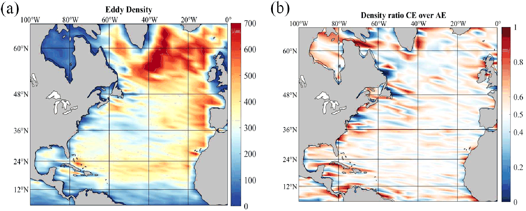
Figure 1. Characteristics of eddy density in the North Atlantic. (a) Spatial distribution of eddy density (grid resolution: 4° × 1°); (b) Ratio of cyclonic to anticyclonic eddy density (grid resolution: 4° × 1°).

Eddy density exhibits a pronounced latitudinal distribution. At high latitudes (48°N–65°N), eddy density exceeds 500, primarily driven by strong shear associated with the westerly drift and the Gulf Stream extension. As a western boundary current, the Gulf Stream is characterized by high velocity and intense shear, which favor eddy generation through both baroclinic and barotropic instabilities (Gaube et al., 2016). The westerly drift enhances the depth of the mixed layer, particularly in winter, promoting baroclinic instability and facilitating eddy formation. Additionally, the low dissipation rates at high latitudes contribute to longer eddy lifespans, resulting in higher eddy densities.

In the mid-latitudes (24°N–48°N), a higher number of eddies (ranging from 400 to 600) is observed along the coasts of Europe and Africa. This region corresponds to the North Atlantic subtropical gyre, where recirculation and current curvature give rise to eddies via barotropic instability (Zhai and Marshall, 2013). The flow field in this region is relatively stable, and eddy generation is primarily driven by large-scale circulation dynamics and thermohaline gradients. The eddy density here is lower than that at higher latitudes but remains higher than in the tropics (Kang and Curchitser, 2013)

In low-latitude regions (12°N–24°N), eddy intensity is significantly reduced, with eddy counts around 400. However, localized high-density zones are observed, such as in the eastern Caribbean Sea. These local maxima can be attributed to island wake effects; for example, the complex topography around the Bahama Islands enhances topographic forcing, which in turn promotes eddy generation. Additionally, instabilities associated with the Equatorial Undercurrent also contribute to eddy formation (Roman-Stork et al., 2021; Pastor-Prieto et al., 2024). Particularly in regions below 12°N, the overall low eddy density is likely associated with strong ocean stratification in the tropics, which suppresses vertical perturbations and inhibits eddy development (Pegliasco et al., 2021).

3.1.2 Eddy propagation distance and speed analysis

As a key dynamic phenomenon in the ocean, mesoscale eddies play a crucial role in cross-regional transport of materials, energy, and momentum. As shown in Figures 2a, b eddy propagation distance exhibits a distinct latitudinal gradient. Specifically, the propagation distance decreases from approximately 300 km at low latitudes (around 5°N) to nearly zero at higher latitudes (48°N–65°N). This pattern arises because low-latitude regions, characterized by weaker planetary effects, allow eddies to propagate westward over longer distances. In contrast, high-latitude areas are influenced by subpolar low-pressure systems and exhibit lower stratification stability, which enhances vertical mixing and dissipation, thereby shortening eddy propagation distances (McWilliams, 1985).

Figure 2

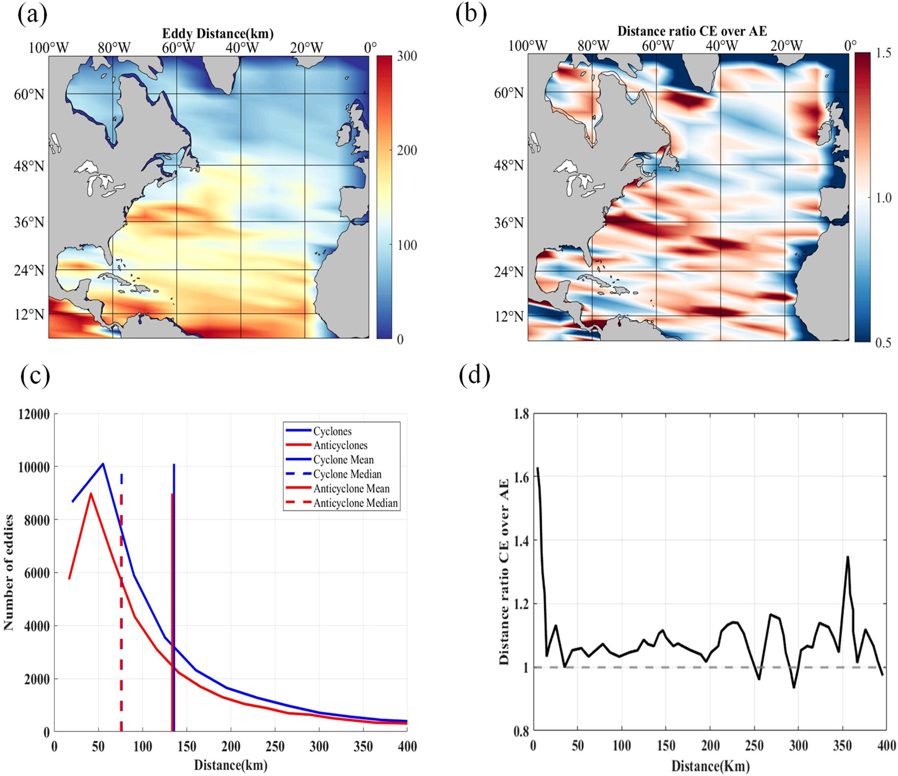
Figure 2. Characteristics of eddy propagation distance in the North Atlantic. (a) Spatial distribution of eddy propagation distance (grid resolution: 5° × 2°); (b) Ratio of cyclonic to anticyclonic propagation distance (grid resolution: 5° × 2°); (c) Relationship between eddy number and propagation distance (blue for cyclones, red for anticyclones); (d) Relationship between the polarity distance ratio and propagation distance.

Further analysis in Figures 2c, d reveals that in the 12°N–36°N region, anticyclonic eddies exhibit significantly longer propagation distances than their cyclonic counterparts, with polarity distance ratios ranging between 1.1 and 1.4. The enhanced stability of anticyclones may be attributed to reduced dissipation associated with downward vertical motion, which favors longer propagation distances (Tamarin-Brodsky and Hadas, 2019). Conversely, in the 5°N–12°N region, where overall propagation distances exceed 250 km, the propagation distance of cyclonic eddies is less than 200 km. This limitation is likely due to upwelling-induced energy loss in cyclonic eddies, resulting in more rapid dissipation and reduced propagation capability (Amores et al., 2017), thus confirming the influence of polarity on eddy propagation characteristics.

Figures 3a, b further illustrate that eddy translation speeds in the western North Atlantic (5°N–48°N) generally exceed 0.1 m/s, with the highest speeds observed in the Gulf Stream extension region (37°N–60°W), where values can reach up to 0.6 m/s. In contrast, at higher latitudes (near 60°N), eddy speeds are relatively low (<0.2 m/s), likely constrained by strong meridional density gradients that act as dynamic barriers to eddy propagation (de Jong and Bower, 2023). The polarity-based velocity ratio indicates that between 48°N and 65°N, the ratio generally exceeds 1.0 and locally reaches as high as 1.5, suggesting that cyclonic eddies move faster than anticyclonic ones in this region. This implies stronger structural stability and a greater potential for long-distance transport. However, in the region around 36°N, 60°W, the ratio drops to approximately 0.5, indicating that anticyclonic eddies are more strongly influenced by the background eastward shear flow (Dufois et al., 2016).

Figure 3

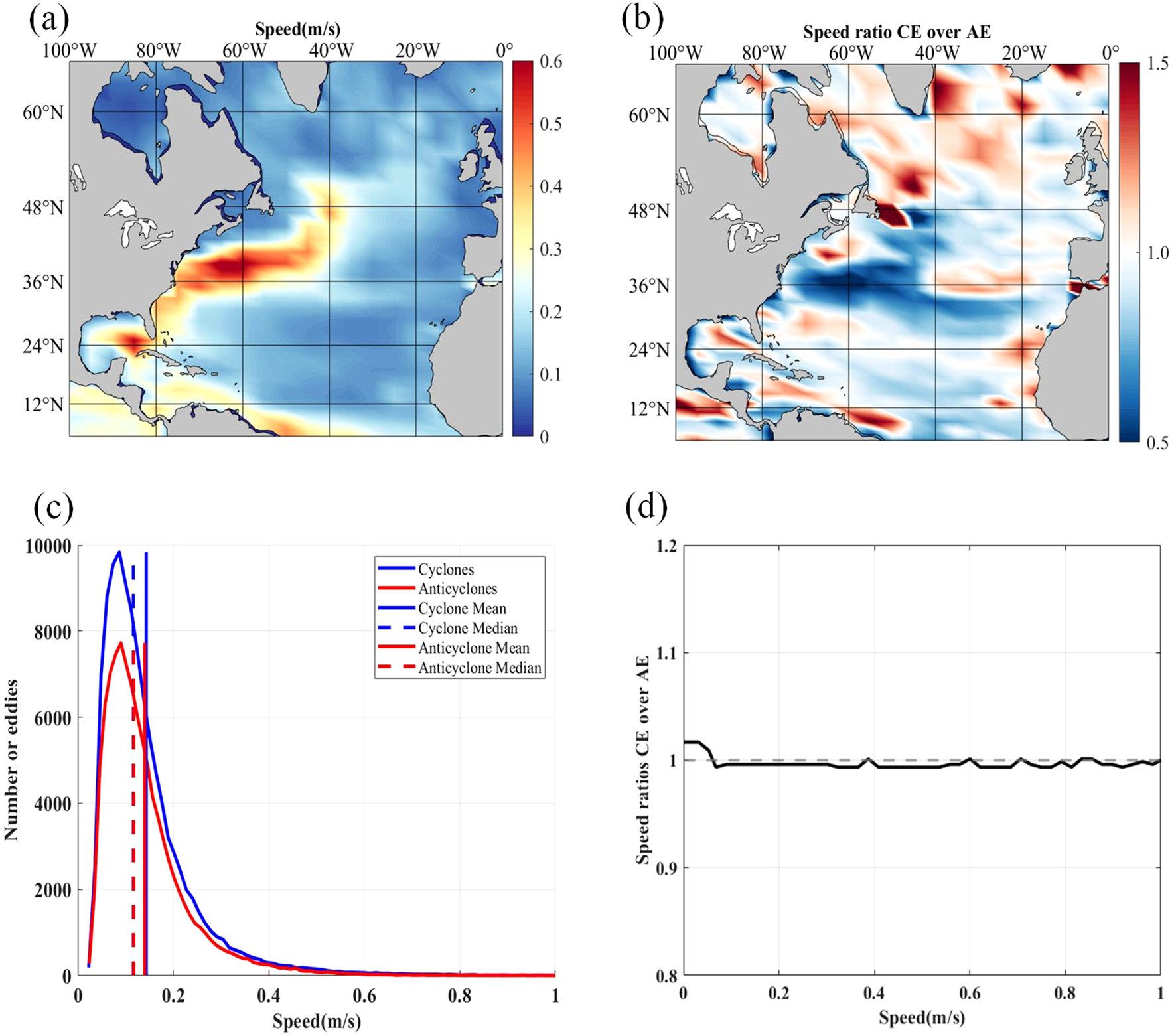
Figure 3. Characteristics of eddy translation speed in the North Atlantic. (a) Spatial distribution of eddy translation speed (grid resolution: 5° × 2°); (b) Ratio of cyclonic to anticyclonic translation speed (grid resolution: 5° × 2°); (c) Relationship between eddy number and translation speed (blue for cyclones, red for anticyclones); (d) Relationship between the polarity speed ratio and translation speed.

The relationship between eddy speed and abundance further reveals that both cyclonic and anticyclonic eddies occur most frequently at a translation speed of approximately 0.09 m/s. As the speed increases, the numerical ratio between the two types of eddies remains close to unity, indicating no strong dominance in propagation speed across most ranges.

3.1.3 Eddy lifetime and generation/decay analysis

As shown in Figure 4, the number of eddies generated in the eastern North Atlantic is significantly higher than that in the western region, exhibiting a characteristic east-west asymmetry. This spatial pattern can be attributed to two primary mechanisms:

Figure 4

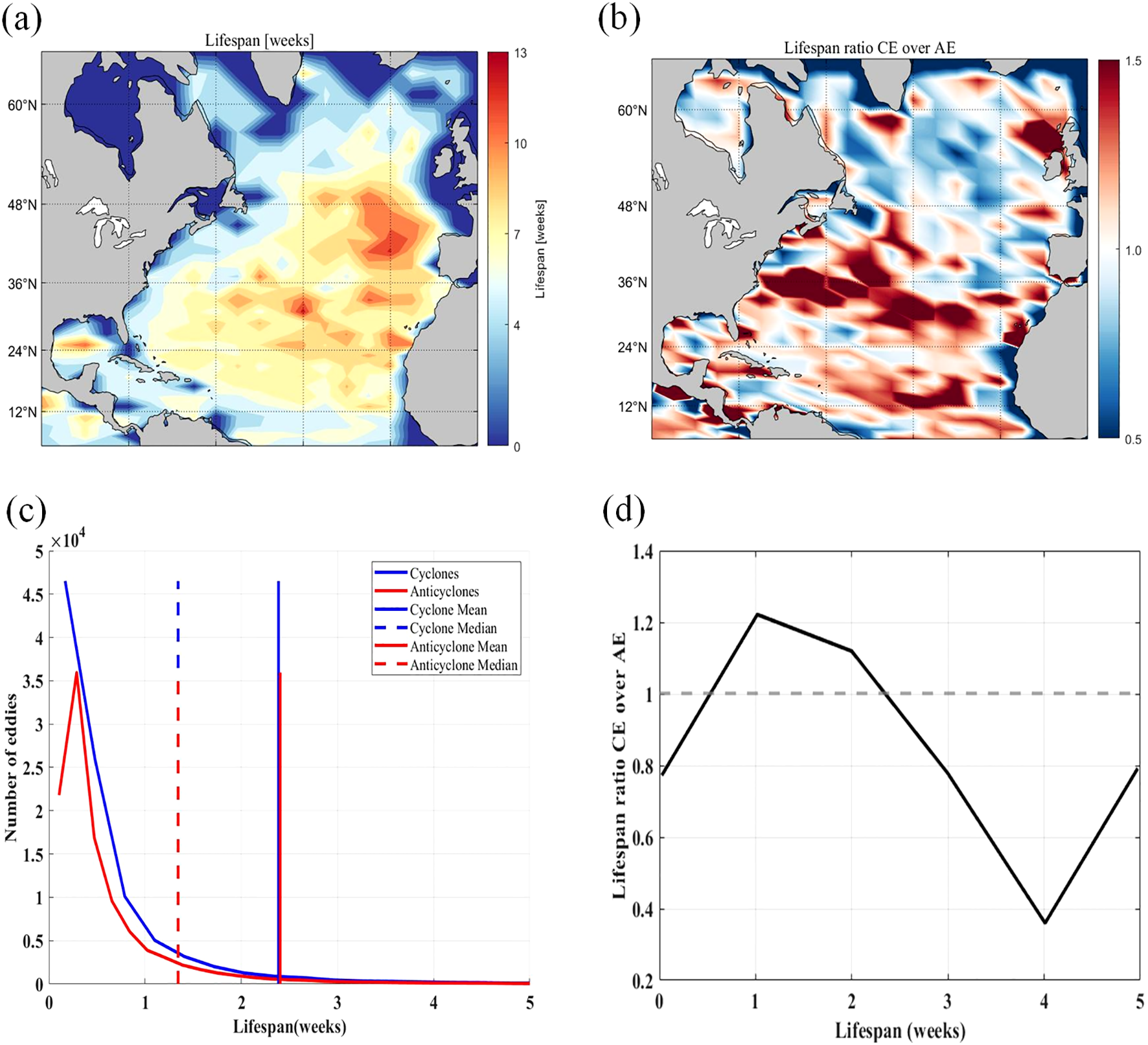
Figure 4. Characteristics of eddy lifecycle in the North Atlantic. (a) Spatial distribution of eddy lifecycle (grid resolution: 5° × 2°); (b) Ratio of cyclonic to anticyclonic lifecycle (grid resolution: 5° × 2°); (c) Relationship between eddy number and lifecycle duration (blue for cyclones, red for anticyclones); (d) Relationship between the polarity lifecycle ratio and lifecycle duration.

1. The interaction between the westerlies and continental topography intensifies eastern boundary upwelling (Yang et al., 2021), creating a stronger baroclinic instability energy source;

2. The westward phase speed of Rossby waves in the eastern Atlantic is relatively slow (approximately 2–3 cm/s), which facilitates the accumulation of wave energy in the eastern basin, thereby triggering eddy formation (Reed et al., 2015). Model results indicate that the removal of wind stress curl input would reduce the eddy generation rate in this region by approximately 35% (Wang et al., 2020).

The generation density of cyclonic eddies in the North Atlantic is notably higher than that in other ocean basins, as illustrated in Figure 5. For example, in the eastern Gulf of Mexico, the annual average number of cyclonic eddies exceeds that in the Kuroshio Extension region of the North Pacific by approximately 40%. This difference may be related to the deep dynamical processes of the Atlantic Meridional Overturning Circulation (AMOC). The AMOC enhances potential vorticity gradients, and through Rhines scale adjustment mechanisms, reduces the characteristic scale of eddy generation, thereby increasing the eddy formation rate per unit area (Rudnick et al., 2015).

Figure 5

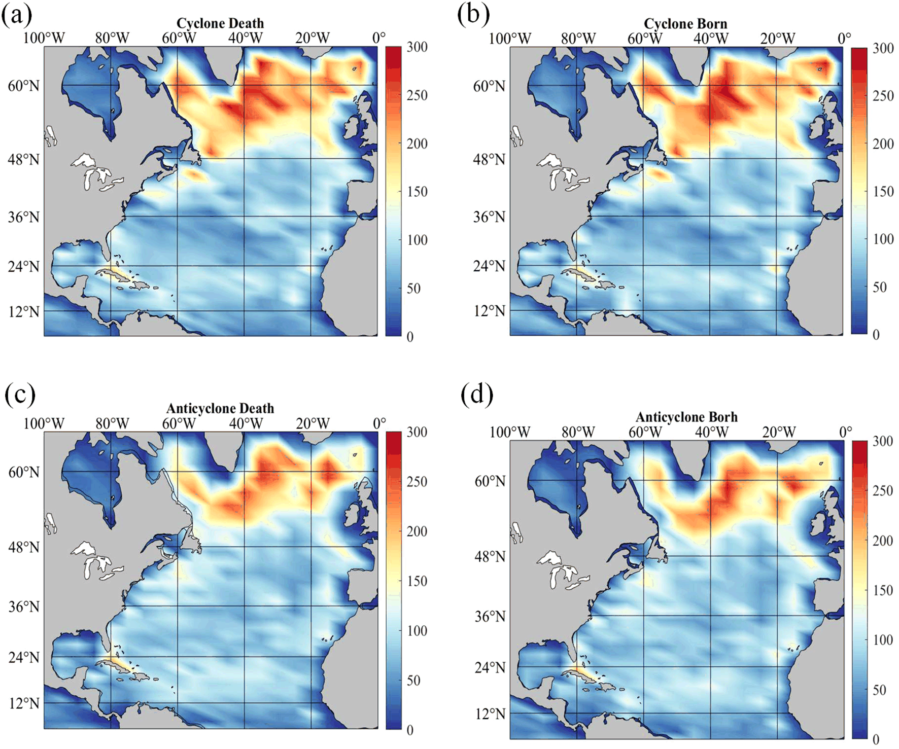
Figure 5. Distribution characteristics of cyclonic and anticyclonic formation and dissipation. (a) Distribution of cyclone dissipation areas; (b) Distribution of cyclone formation areas; (c) Distribution of anticyclone dissipation areas; (d) should be the distribution of anticyclone formation areas.

3.1.4 Eddy Kinetic Energy and root mean square of sea level anomalies

Mesoscale eddies are important carriers of energy transport and material exchange in the ocean, and their intensity can typically be quantified using Eddy Kinetic Energy (EKE) and the Root Mean Square of Sea Level Anomalies (SSHA RMS). Influenced by the Gulf Stream system, western boundary currents, and AMOC, previous studies have shown that the Gulf Stream generates strong eddies through baroclinic instability, with EKE reaching up to 1200 cm²/s², indicating high kinetic energy input (De Castro et al., 2018; Fraser et al., 2024). AMOC strengthens vertical mixing and enhances eddy energy transport, potentially regulating climate through heat and salinity gradients (Engida et al., 2016). As a result, the North Atlantic is recognized as one of the most active mesoscale eddy regions globally (Zhang et al., 2012).

As shown in Figure 6a, EKE in the North Atlantic ranges from 0 to 1200 cm²/s², with high values concentrated in the Gulf Stream extension and the North Atlantic Current region (24°N–48°N, 40°W–60°W). Figure 6b illustrates a gradual increase in SSHA along the American coast between 24°N and 48°N, with peak values reaching up to 10 cm. Additionally, in the subpolar region (around 60°N), enhanced SSHA may be closely related to the positive phase of the North Atlantic Oscillation (NAO), during which strengthened westerlies drive sea surface height accumulation toward the polar regions (Li et al., 2012).

Figure 6

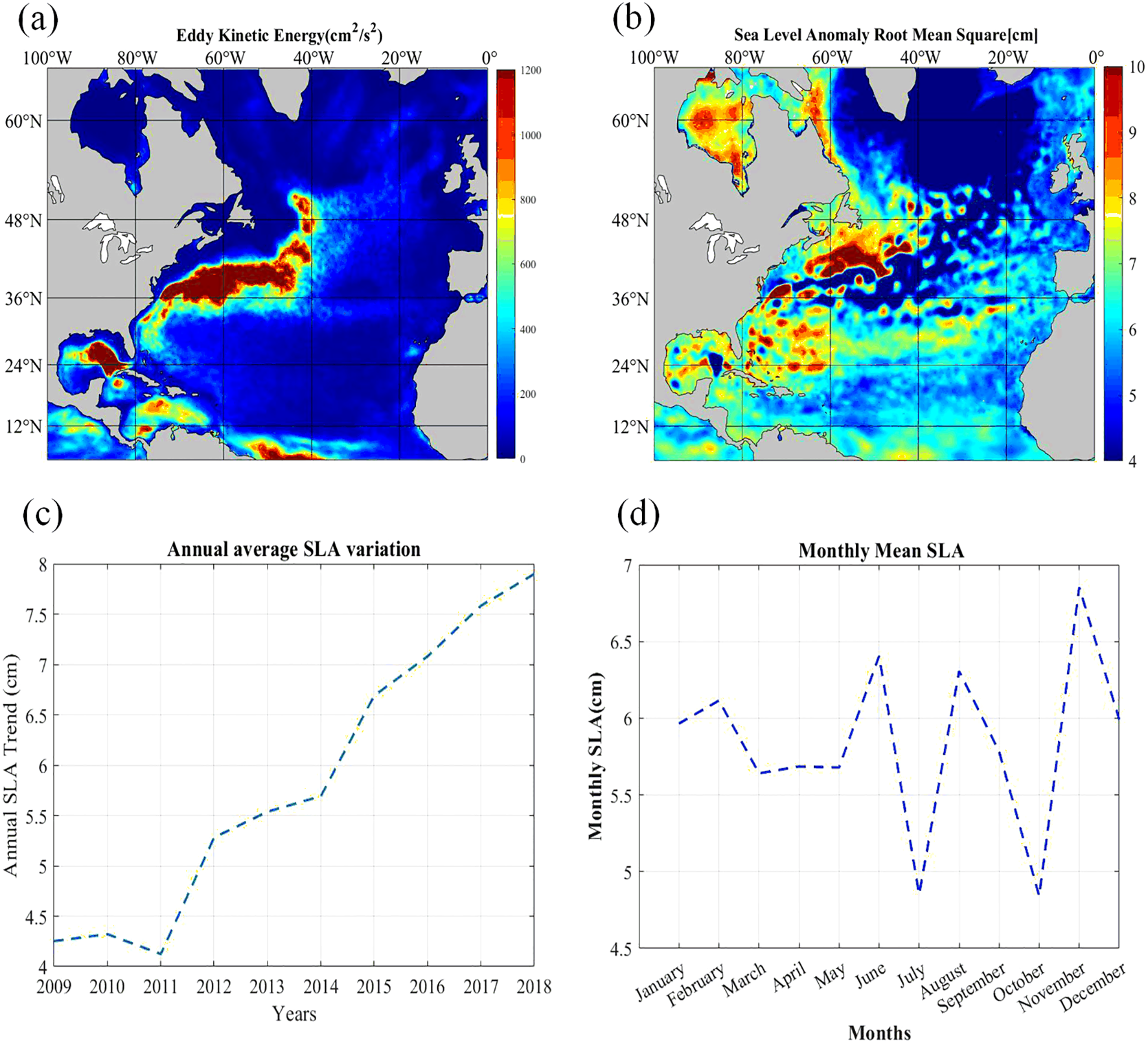
Figure 6. Distribution characteristics of eddy kinetic energy and sea level anomalies. (a) Distribution of eddy kinetic energy; (b) Distribution of sea level anomaly (SLA) regions; (c) Annual mean variation of SLA (line plot); (d) Monthly mean variation of SLA (line plot).

Figures 6c, d show that on an interannual scale, SSHA exhibited an overall increasing trend from 2009 to 2018, with a slight decrease only during 2010–2011; all other years showed varying degrees of increase. On a monthly scale, SSHA displayed pronounced seasonal variability. Compared to the baseline value of 5.5 cm, SSHA RMS rises sharply during October and November, reaching a peak of approximately 6.8 cm, whereas July and August show the lowest values, around 4.8 cm. This seasonal fluctuation is closely linked to wind forcing—i.e., intensified storm activity in autumn and reduced wind stress in summer—indicating a strong seasonal modulation of eddy activity in this region.

3.1.5 Eddy intensity

In the topographic region of the North Atlantic (2°N–18°N), mesoscale eddies exhibit relatively large mean radii, generally exceeding 70 km. Around 36°N, eddies in the mid-ocean region typically range from 60 to 70 km in radius, while at higher latitudes (north of 48°N), the average radius decreases to below 50 km, as shown in Figure 7a. Combined with the polarity radius ratio displayed in Figure 7b (values greater than 1 in the southern section), it is evident that large-radius eddies in the southern region are able to maintain higher energy density, which helps them resist background flow shear and sustain longer propagation distances.

Figure 7

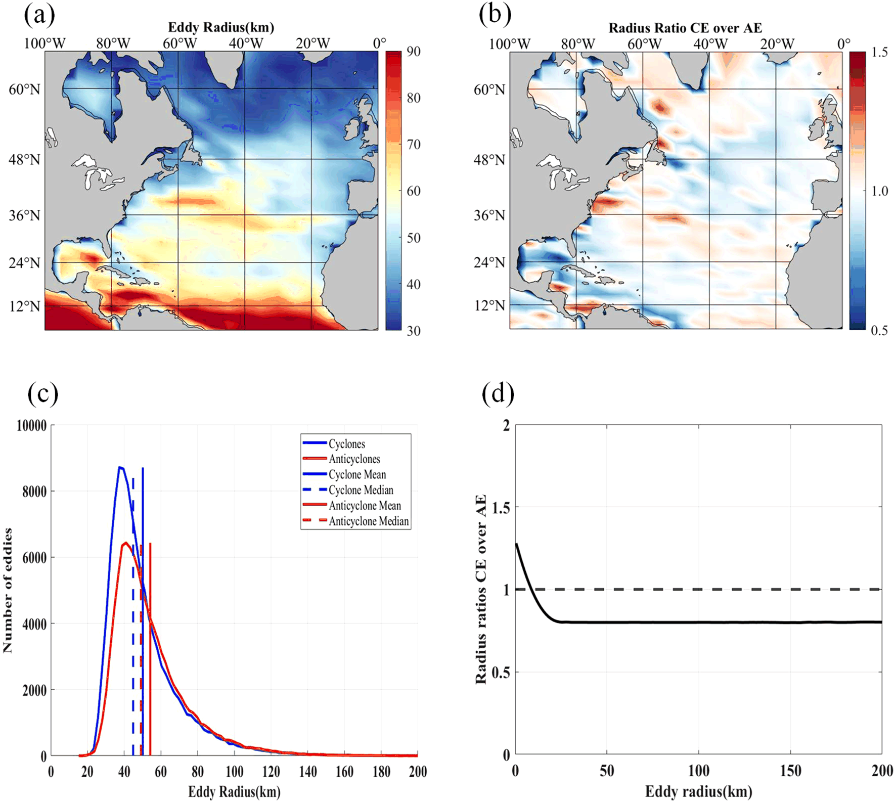
Figure 7. Characteristics of eddy radius in the North Atlantic. (a) Spatial distribution of eddy radius (grid resolution: 5° × 2°); (b) Ratio of cyclonic to anticyclonic eddy radius (grid resolution: 5° × 2°); (c) Relationship between eddy number and radius size (blue for cyclones, red for anticyclones); (d) Relationship between the polarity radius ratio and radius size.

Figure 7c shows the relationship between eddy radius and abundance during 2009–2018. Regardless of polarity, both cyclonic and anticyclonic eddies are most frequently observed around a radius of 40 km. Although the total number of cyclonic eddies slightly exceeds that of anticyclonic eddies, both types exhibit a similar distribution pattern: small-radius eddies are more common, while among eddies with radii greater than 50 km, anticyclones dominate. Figure 7d further indicates that when eddy radius exceeds 40 km, the cyclone-to-anticyclone number ratio drops below 0.8, suggesting that large-radius eddies are primarily anticyclonic. In contrast, for eddies smaller than 40 km, the ratio approaches 1.2, indicating a dominance of cyclonic eddies. This implies that anticyclonic eddies are more readily captured by background flow fields in western boundary regions (for exempli gratia the Gulf Stream), where their downward motion helps concentrate energy toward the core, enlarging the radius and enhancing structural stability (Laxenaire et al., 2019). In contrast, small-radius cyclonic eddies are driven by upwelling-induced surface divergence, resulting in faster energy dissipation and more limited propagation.

Figure 8 shows that during 2009–2018, eddy intensity in the central and western North Atlantic (40°W–80°W, 30°N–48°N) generally exceeds 0.2 cm/km, with peak values reaching 0.35 cm/km in the Gulf Stream detachment region (36°N–40°N, 80°W–60°W). In comparison, eddy intensity in the eastern basin (east of 20°W) drops sharply to below 0.1 cm/km, with a spatial distribution pattern closely matching that of eddy kinetic energy. This phenomenon is strongly associated with the high-energy input from the Gulf Stream, which generates intense eddies via baroclinic instability. The velocity shear and potential vorticity gradients in this region provide the dynamic foundation for eddy intensification. The average eddy intensity in the Gulf Stream extension reaches 0.32 cm/km, significantly higher than that in the eastern basin (0.08 cm/km), reaffirming the “strong west–weak east” distribution pattern (Ioannou et al., 2024).

Figure 8

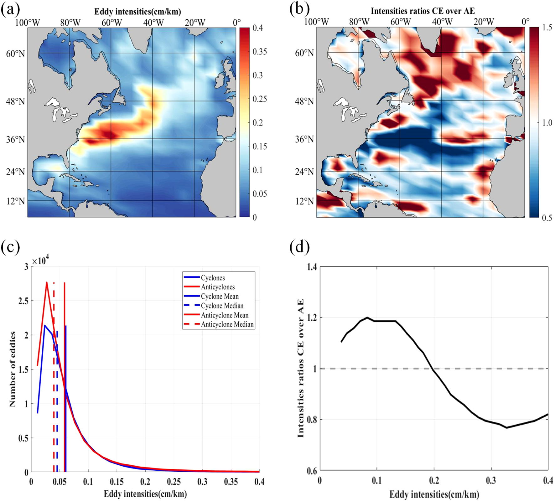
Figure 8. Characteristics of eddy intensity in the North Atlantic. (a) Spatial distribution of eddy intensity (grid resolution: 5° × 2°); (b) Ratio of cyclonic to anticyclonic eddy intensity (grid resolution: 5° × 2°); (c) Relationship between eddy number and intensity size (blue for cyclones, red for anticyclones); (d) Relationship between the polarity intensity ratio and intensity size.

As shown in Figure 9a, eddy amplitude peaks in the 36°N–48°N zone, reaching values as high as 30 cm. The spatial distribution of amplitude closely aligns with that of eddy intensity and eddy kinetic energy. Cyclonic eddies generally exhibit higher amplitudes than anticyclonic ones, as demonstrated in Figure 9b. In the high-latitude region (48°N–65°N), the polarity amplitude ratio is mostly above 1.0, and in some areas exceeds 1.5, indicating that cyclonic eddies have significantly higher amplitudes than anticyclonic eddies in these latitudes (Figure 9c). However, near 36°N (40°W–60°W), the ratio drops to approximately 0.5, suggesting a dominance of anticyclonic amplitudes in this region, whereas along the coast, cyclonic eddies tend to dominate.

Figure 9

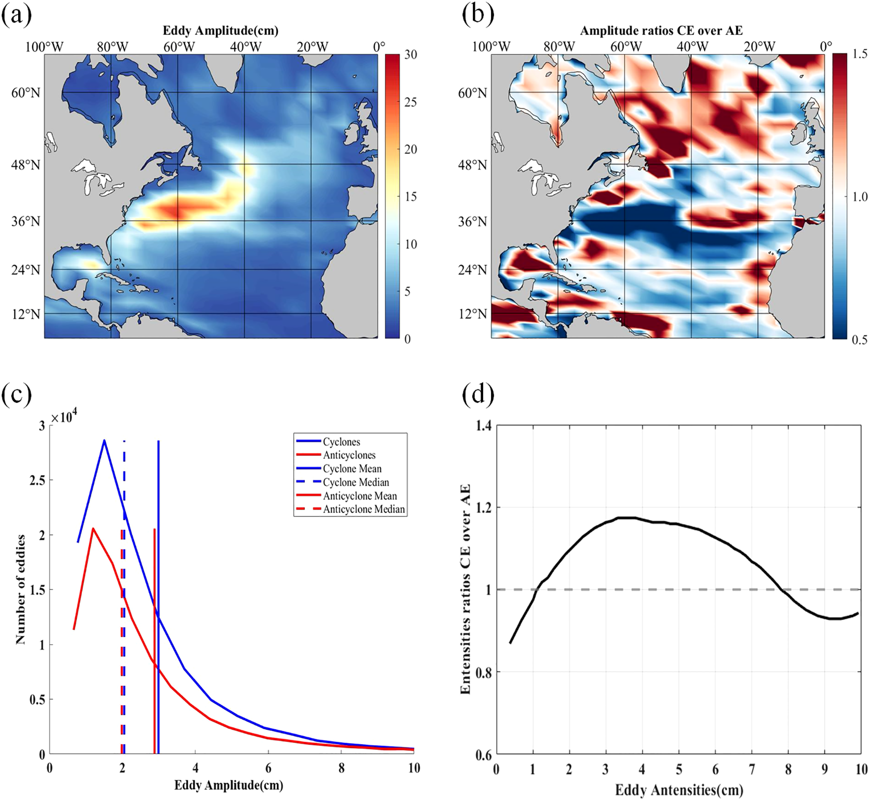
Figure 9. Characteristics of eddy amplitude in the North Atlantic. (a) Spatial distribution of eddy amplitude (grid resolution: 5° × 2°); (b) Ratio of cyclonic to anticyclonic eddy amplitude (grid resolution: 5° × 2°); (c) Relationship between eddy number and amplitude size (blue for cyclones, red for anticyclones); (d) Relationship between the polarity amplitude ratio and amplitude size.

In terms of amplitude-abundance distribution, for small-amplitude eddies (<5 cm), the number of cyclonic eddies is about 1.2 times that of anticyclonic eddies. In contrast, for large-amplitude eddies (>15 cm), the proportion of anticyclones increases to 45%. Although the average amplitude of cyclonic eddies (12.5 cm) is slightly higher than that of anticyclones (11.8 cm), the median difference is minimal—9.2 cm for cyclones and 9.0 cm for anticyclones, as shown in Figure 9d. These results demonstrate that the eddy amplitude distribution in the North Atlantic is representative and follows typical patterns.

3.2 Relationship between mesoscale eddies and chlorophyll-a concentration

3.2.1 Surface characteristics of chlorophyll-a under eddy influence and its temporal-spatial distribution

The surface distribution of chlorophyll-a (Chl-a) in the North Atlantic exhibits pronounced zonal patterns and regional heterogeneity. Its concentration gradients are jointly regulated by physical factors such as circulation structures and mixed layer depth (MLD), as well as biogeochemical processes including nutrient supply and community composition. Spatially, three primary zones can be identified, as illustrated in Figure 10:

Figure 10

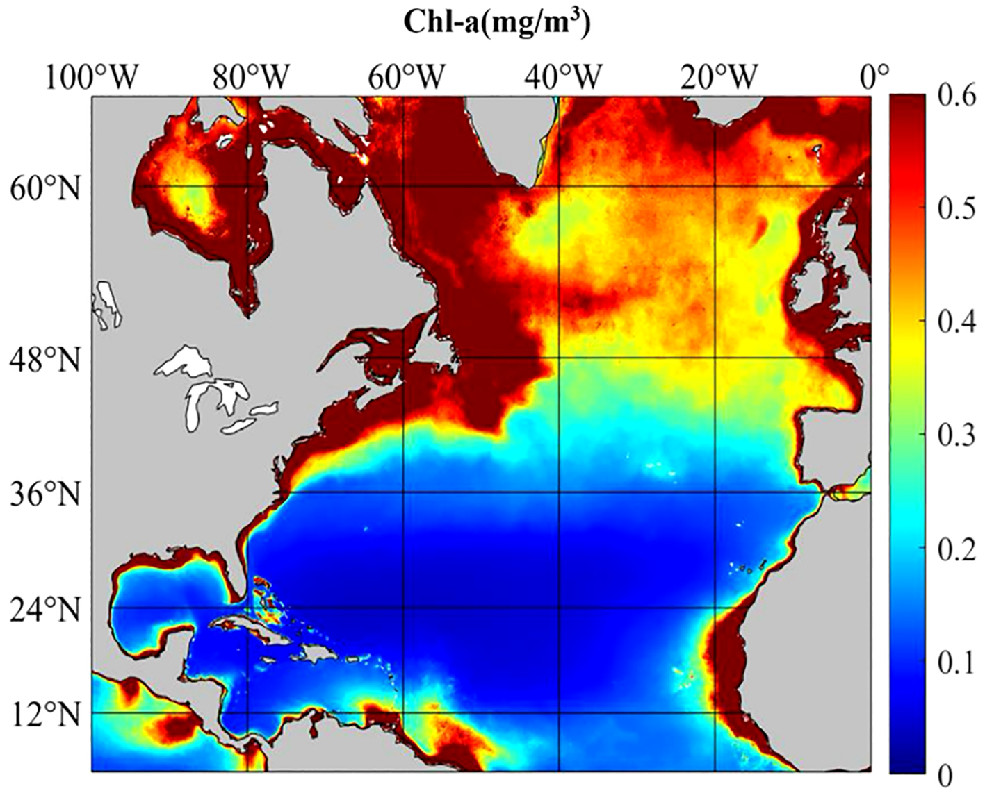
Figure 10. Spatial distribution of surface chlorophyll-a concentration in the North Atlantic.

1. High-Latitude Region (36°N ~ 65°N):

Influenced by deep winter mixing and improved light conditions during spring, intense phytoplankton blooms occur, with Chl-a peak concentrations reaching up to 0.6 mg/m³ (in the Labrador Sea). High concentrations are typically located near continental shelves and in areas of frequent eddy activity.

2. Mid-Latitude to Low-Latitude Region (5°N ~ 36°N):

Dominated by anticyclonic eddies, this region exhibits strong stratification and nutrient depletion, resulting in low Chl-a concentrations ranging from 0 to 0.2 mg/m³. However, nearshore waters show relatively elevated concentrations due to coastal upwelling.

3. Coastal Transition Zones:

Including the eastern coasts of North America and parts of the European continental shelf, where Chl-a concentrations are generally higher due to terrestrial input and upwelling processes.

Seasonal variations in Chl-a are jointly controlled by photosynthetically active radiation (PAR), MLD, and nutrient transport. As shown in Figure 11, monthly mean Chl-a concentrations increase rapidly in spring (March–May), reaching 0.5 ± 0.1 mg/m³ due to enhanced light and shallower mixed layers. In summer (June–August), peak values of around 0.57 mg/m³ occur under high irradiance and moderate nutrient availability. During autumn (September–November), deepening of the mixed layer and nutrient replenishment lead to a secondary peak (0.45 mg/m³). In winter (December–February), Chl-a drops to its lowest level (~0.31 mg/m³) due to light limitation. On an interannual scale (Figure 11b), higher Chl-a values were observed during 2010–2012. In contrast, from 2013–2015, Chl-a declined under the influence of a negative NAO phase and weakened vertical mixing, indicating modulation by climatic modes.

Figure 11

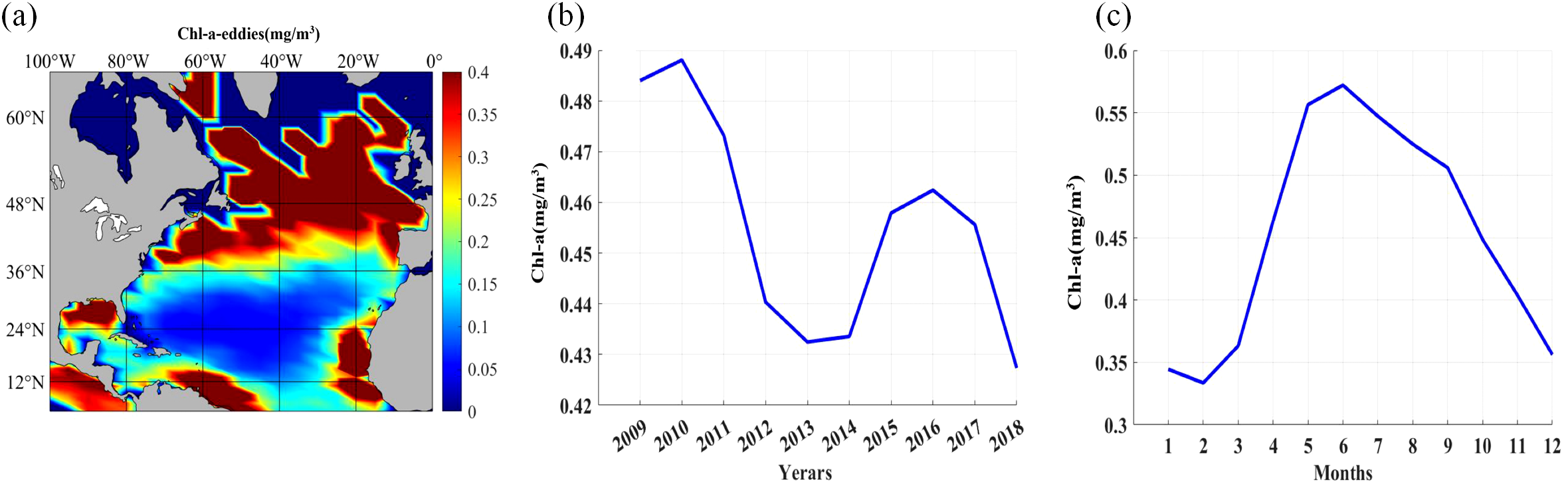
Figure 11. Relationship between chlorophyll-a and Eddy. (a) Spatial distribution characteristics of chlorophyll-a and eddy; (b) Annual mean variation of chlorophyll-a concentration from 2009 to 2018; (c) Monthly mean variation of chlorophyll-a concentration from 2009 to 2018.

To further verify the influence of eddies on Chl-a dynamics, four representative eddies from different seasons and regions were analyzed, including both cyclonic and anticyclonic types (Figure 12). In cyclonic eddies (Figures 12a, b), Chl-a concentrations increased significantly within 0.5R of the eddy core, with anomalies reaching up to +0.2 mg/m³, indicating enhanced vertical nutrient transport. Conversely, anticyclonic eddies (Figures 12c, d) generally exhibited reduced Chl-a concentrations in the core region (20%–40% lower), with gradual recovery toward the periphery. This spatial structure validates the statistical patterns discussed earlier and confirms their physical consistency across different latitudes and seasons.

Figure 12

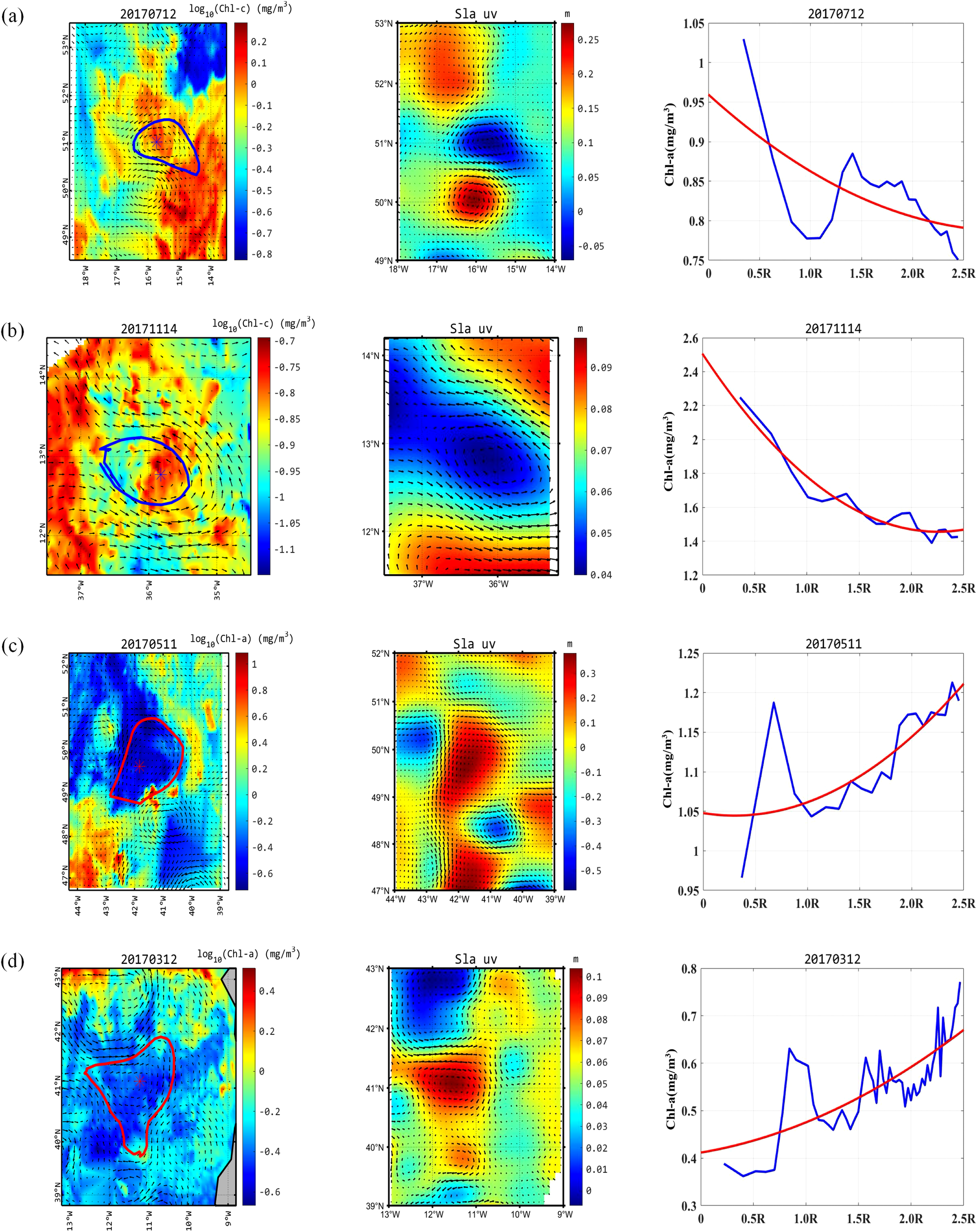
Figure 12. Relationship between eddy distribution and SLA in the North Atlantic. (a) (Left) Spatial distribution of surface chlorophyll-a for cyclone ID NA_031127, with background color representing the logarithm of surface chlorophyll concentration; (Middle) Schematic of sea level anomaly in the region; (Right) Variation of surface chlorophyll-a concentration (unit: mg/m³) with eddy radius, with blue representing chlorophyll data and red representing fitted data. (b) (Left) Spatial distribution of surface chlorophyll-a for cyclone ID NA_031617, with background color representing the logarithm of surface chlorophyll concentration; (Middle) Schematic of sea level anomaly in the region; (Right) Variation of surface chlorophyll-a concentration (unit: mg/m³) with eddy radius. (c) (Left) Spatial distribution of surface chlorophyll-a for anticyclone ID NA_030888, with background color representing the logarithm of surface chlorophyll concentration; (Middle) Schematic of sea level anomaly in the region; (Right) Variation of surface chlorophyll-a concentration (unit: mg/m³) with eddy radius. (d) (Left) Spatial distribution of surface chlorophyll-a for anticyclone ID NA_030690, with background color representing the logarithm of surface chlorophyll concentration; (Middle) Schematic of sea level anomaly in the region; (Right) Variation of surface chlorophyll-a concentration (unit: mg/m³) with eddy radius.

In summary, mesoscale eddies regulate primary productivity through multiple mechanisms, including modulation of vertical nutrient fluxes, disruption of the thermocline, and alteration of PAR penetration. Cyclonic eddies tend to enhance Chl-a concentrations most significantly during spring to early summer, when light and temperature conditions are favorable. Anticyclonic eddies, on the other hand, are more likely to induce strong stratification and suppress productivity during summer and autumn, reflecting distinct physical–ecological coupling mechanisms based on eddy polarity and seasonal context.

3.2.2 Vertical characteristics of chlorophyll-a concentration

Figure 13 illustrates the vertical structural features of cyclonic and anticyclonic eddies in the North Atlantic, including original profiles and anomaly fields of density, temperature, and salinity. In terms of density, cyclonic eddies exhibit decreased density in the upper layer (0–200 m), indicating the dominance of upwelling processes, with the strongest negative anomalies near the surface. In contrast, anticyclonic eddies show enhanced density in the same depth range, reflecting a downwelling structure. The temperature profiles reveal a cold-core pattern in cyclonic eddies (surface cooling of approximately 1°C) and a distinct warm-core structure in anticyclonic eddies (warming exceeding 1°C), further supporting the contrasting vertical motions between the two eddy types. Salinity data show a positive salinity anomaly in anticyclonic eddies within the upper 150 m, with maximum values exceeding 0.4 g/kg. Conversely, cyclonic eddies display a negative salinity anomaly (less than −0.4 g/kg) at mid-depths (200–400 m), likely associated with the disturbance of regional water masses, such as subtropical high-salinity water or cold intermediate waters. These structural differences highlight the role of mesoscale eddies in modulating the local physical environment, especially in regulating nutrient supply within the euphotic layer (Cobb and Czaja, 2019; Müller et al., 2019). The presence of a “double-peak” pattern in temperature profiles further indicates vertical displacement of isotherms caused by eddies, which may significantly impact nutrient redistribution.

Figure 13

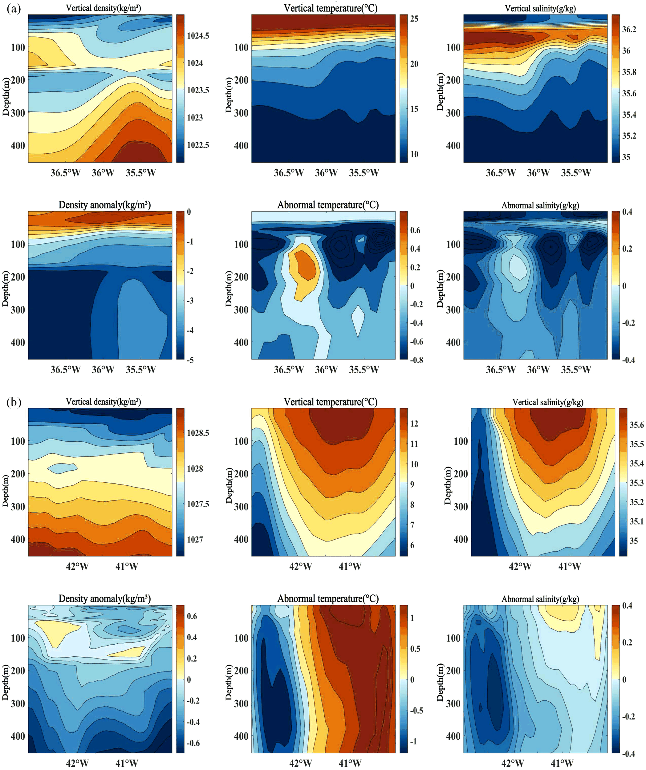
Figure 13. Vertical characterization of eddy in the North Atlantic. (a) Vertical profile of sea water density (left), temperature (middle), and salinity (right) anomalies across the center of cyclone ID NA_031617 along the east-west direction. (b) Vertical profile of sea water density (left), temperature (middle), and salinity (right) anomalies across the center of anticyclone ID NA_030888 along the east-west direction.

Figure 14 presents the vertical structure and anomaly response of Chl-a concentration in cyclonic and anticyclonic eddies (according to Figure (a)-(b)). In cyclonic eddies, a pronounced Chl-a peak is observed at depths of 50–70 m, with concentrations reaching 0.35–0.4 mg/m³ and positive anomalies exceeding +0.1 mg/m³. This indicates that upwelling transports nutrients into the photic zone, greatly enhancing phytoplankton growth. In contrast, anticyclonic eddies exhibit strong negative Chl-a anomalies (< −0.1 mg/m³) at similar depths, suggesting that intensified stratification and downwelling suppress nutrient supply and primary productivity. Horizontal cross-sections show that the anomaly fields are concentrated in the eddy cores and gradually weaken toward the periphery, reflecting the spatial organization of vertical transport processes. These findings demonstrate that eddies of opposite polarity significantly influence the subsurface phytoplankton distribution in the North Atlantic by regulating the vertical nutrient structure. The internal vertical structure of eddies plays a critical role in modulating surface Chl-a concentrations.

Figure 14

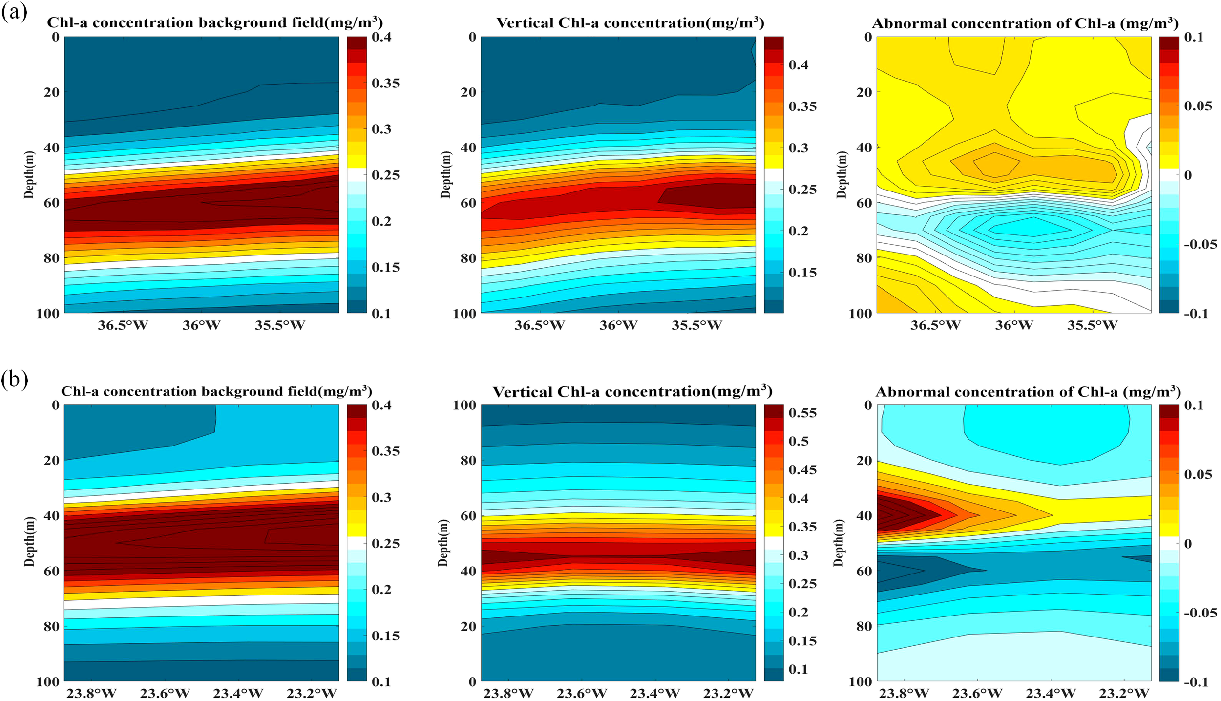
Figure 14. Vertical characterization of chlorophyll-a anomalies in Eddies of the North Atlantic. (a) Chlorophyll-a concentration background field (left), vertical chlorophyll-a concentration (middle), and chlorophyll-a concentration anomaly (right) for cyclone ID NA_031617. (b) Chlorophyll-a concentration background field (left), vertical chlorophyll-a concentration (middle), and chlorophyll-a concentration anomaly (right) for anticyclone ID NA_031604.

Seasonal variations of Chl-a in the North Atlantic are jointly regulated by light availability, temperature, and nutrient supply (Song et al., 2025). During spring, favorable light and temperature conditions drive phytoplankton blooms, forming seasonal Chl-a maxima. In summer, surface warming enhances stratification, and nutrient resupply continues to elevate Chl-a concentrations. In autumn, deepening of the mixed layer facilitates nutrient replenishment, resulting in a secondary peak. In winter, limited light and low temperatures reduce productivity, causing Chl-a levels to drop to their annual minimum. Interannual variability is also evident, and Chl-a fluctuations are closely coupled with climatic forcing factors such as the North Atlantic Oscillation (NAO) and anthropogenic influences. Under global warming, elevated atmospheric CO₂ concentrations—driven by human activity—may alter atmospheric circulation, influence NAO phases, and indirectly affect phytoplankton photosynthesis. Simultaneously, ocean acidification may suppress calcifying phytoplankton and alter community structure, ultimately impacting Chl-a concentrations (Abbasi and Abbasi, 2011; Sommer et al., 2015). Moreover, enhanced surface stratification and changes in wind forcing can significantly affect mesoscale eddy intensity, frequency, and vertical transport capacity, influencing nutrient supply in oligotrophic zones and reshaping phytoplankton distributions and ecosystem functioning at the regional scale.

4 Conclusion

This study, based on multi-source satellite remote sensing data and using velocity vector geometric identification and temporal-spatial matching methods, automatically tracked mesoscale eddies in the North Atlantic from 2009 to 2018. By combining multi-source observational data, we systematically analyzed the dynamical characteristics of eddies in the region, the spatial distribution of sea surface chlorophyll, and the vertical regulatory mechanisms. The results show that mesoscale eddy activity in the North Atlantic exhibits significant spatial heterogeneity, with the Gulf Stream extension being the primary energy source for eddy formation. Cyclonic eddies have longer lifecycles and higher vertical transport efficiency than anticyclonic eddies. Cyclonic eddies dominate nutrient supply through vertical entrainment, while anticyclonic eddies rely on dynamic convergence, with the edge shear process having a stronger regulatory effect on biological distribution than the eddy core. Eddy-driven Chl-a variations contribute to 20% ± 5% of the primary productivity in the North Atlantic, and their carbon export effect plays an important role in regional climate regulation.

However, the study faces some limitations, such as the significant cloud contamination of satellite chlorophyll data (with more than 40% missing data), and the low temporal resolution of Argo profile observations (approximately 10 days), making it difficult to capture rapid changes in eddies. Additionally, existing biogeochemical models are not accurate enough to depict submesoscale processes, leading to lower chlorophyll simulations. Future research needs to improve the characterization of ocean eco-dynamic processes through the integration of high-resolution numerical simulations, multi-source data assimilation, and cross-scale process studies, thereby enabling a more accurate response to changes in marine ecosystems.

Data availability statement

The original contributions presented in the study are included in the article/supplementary material. Further inquiries can be directed to the corresponding authors.

Author contributions

JC: Resources, Methodology, Supervision, Validation, Project administration, Writing – review & editing, Investigation, Software, Writing – original draft, Formal Analysis, Visualization, Data curation. JS: Data curation, Visualization, Software, Investigation, Writing – review & editing, Resources, Conceptualization, Validation, Project administration, Funding acquisition, Supervision, Formal Analysis, Writing – original draft, Methodology. SQ: Resources, Investigation, Visualization, Supervision, Validation, Data curation, Writing – review & editing. YL: Supervision, Investigation, Validation, Writing – review & editing, Data curation, Visualization.

Funding

The author(s) declare that financial support was received for the research and/or publication of this article. Research Project: Study on the Protection of Terrain and Geomorphology and Ecological Service Value of Sea Areas and Islands in Jiangsu Province (Project Number: JSZRKJ202421). This research was also supported by the project titled “Key Technologies for Subsea Shallow Stratum Detection of 300,000-ton Channel in Lianyungang,” which is part of the Lianyungang Municipal Key R&D Program (Industrial Foresight and Key Core Technologies), Project Number: 22CY080.

Conflict of interest

The authors declare that the research was conducted in the absence of any commercial or financial relationships that could be construed as a potential conflict of interest.

Generative AI statement

The author(s) declare that no Generative AI was used in the creation of this manuscript.

Publisher’s note

All claims expressed in this article are solely those of the authors and do not necessarily represent those of their affiliated organizations, or those of the publisher, the editors and the reviewers. Any product that may be evaluated in this article, or claim that may be made by its manufacturer, is not guaranteed or endorsed by the publisher.

References

Abbasi T. and Abbasi S. A. (2011). Ocean acidification: the newest threat to the global environment. Crit. Rev. Environ. Sci. Technol. 41, 1601–1663. doi: 10.1080/10643389.2010.481579

Crossref Full Text | Google Scholar

Amores A., Melnichenko O. V., and Maximenko N. (2017). Coherent mesoscale eddies in the North Atlantic subtropical gyre: 3-D structure and transport with application to the salinity maximum. J. Phys. Oceanography 47, 2307–2321. doi: 10.1175/JPO-D-17-0030.1

Crossref Full Text | Google Scholar

Androulidakis Y., Kourafalou V., Le Hénaff M., Kang H., Ntaganou N., and Hu C. (2020). Gulf Stream evolution through the Straits of Florida: The role of eddies and upwelling near Cuba. Ocean Dynamics 70, 1005–1032. doi: 10.1007/s10236-020-01381-5

Crossref Full Text | Google Scholar

Browning T. J., Al-Hashem A. A., Hopwood M. J., Engel A., Belkin I. M., Wakefield E. D., et al. (2021). Iron regulation of north atlantic eddy phytoplankton productivity. Geophysical Res. Lett. 48, e2020GL091403. doi: 10.1029/2020GL091403

Crossref Full Text | Google Scholar

Chen Y., Li Q. P., and Yu J. (2022). Submesoscale variability of subsurface chlorophyll-a across eddy-driven fronts by glider observations. Prog. Oceanography 209, 102905. doi: 10.1016/j.pocean.2022.102905

Crossref Full Text | Google Scholar

Cobb A. and Czaja A. (2019). Mesoscale signature of the North Atlantic Oscillation and its interaction with the ocean. Geophysical Res. Lett. 46, 5575–5581. doi: 10.1029/2018GL080744

Crossref Full Text | Google Scholar

Cornec M., Laxenaire R., Speich S., and Claustre H. (2021). Impact of mesoscale eddies on deep chlorophyll maxima. Geophysical Res. Lett. 48, e2021GL093470. doi: 10.1029/2021GL093470

PubMed Abstract | Crossref Full Text | Google Scholar

De Castro A. I., Six J., Plant R. E., and Peña J. M. (2018). Mapping crop calendar events and phenology-related metrics at the parcel level by object-based image analysis (OBIA) of MODIS-NDVI time-series: A case study in central california. Remote Sens. 10, 1745. doi: 10.3390/rs10111745

Crossref Full Text | Google Scholar

de Jong M. F. and Bower A. S. (2023). Deep ocean circulation in the subpolar North Atlantic observed by acoustically-tracked floats. Prog. Oceanography 217, 102975. doi: 10.1016/j.pocean.2023.102975

Crossref Full Text | Google Scholar

Drouin K. L., Lozier M. S., Beron-Vera F. J., Miron P., and Olascoaga M. J. (2022). Surface pathways connecting the South and North Atlantic oceans. Geophysical Res. Lett. 49, e2021GL096646. doi: 10.1029/2021GL096646

Crossref Full Text | Google Scholar

Dufois F., Hardman-Mountford N. J., Greenwood J., Richardson A. J., Feng M., and Matear R. J. (2016). Anticyclonic eddies are more productive than cyclonic eddies in subtropical gyres because of winter mixing. Sci. Adv. 2. doi: 10.1126/sciadv.1600282

PubMed Abstract | Crossref Full Text | Google Scholar

Engida Z., Monahan A., Ianson D., and Thomson R. E. (2016). Remote forcing of subsurface currents and temperatures near the northern limit of the California Current System, J. Geophys. Res. Oceans 121, 7244–7262. doi: 10.1002/2016JC011880

Crossref Full Text | Google Scholar

Faghmous J., Frenger I., Yao Y., Warmka R., Lindell A., and Kumar V.. (2015). A daily global mesoscale ocean eddy dataset from satellite altimetry. Sci. Data 2, 150028. doi: 10.1038/sdata.2015.28

PubMed Abstract | Crossref Full Text | Google Scholar

Follows M. and Dutkiewicz S. (2001). Meteorological modulation of the North Atlantic spring bloom. US JGOFS Synthesis. Modeling. Project.: Phase. 1 49, 321–344. doi: 10.1016/S0967-0645(01)00105-9

Crossref Full Text | Google Scholar

Fraser N. J., Fox A. D., Cunningham S. A., Rath W., Schwarzkopf F. U., and Biastoch A. (2024). Vertical velocity dynamics in the north atlantic and implications for AMOC. J. Phys. Oceanography 54, 2011–2024. doi: 10.1175/JPO-D-23-0229.1

Crossref Full Text | Google Scholar

Fu L.-L. and Morrow R. (2013). “Chapter 4—Remote sensing of the global ocean circulation,” in International geophysics, vol. 103 . Eds. Siedler G., Griffies S. M., Gould J., and Church &J.A. (Academic Press), 83–111). doi: 10.1016/B978-0-12-391851-2.00004-0

Crossref Full Text | Google Scholar

Gaube P., Chelton D. B., Strutton P. G., and Behrenfeld M. J. (2016). Anticyclonic eddies are more productive than cyclonic eddies in subtropical gyres because of winter mixing. Sci. Adv. 2, e1600282. doi: 10.1126/sciadv.1600282

PubMed Abstract | Crossref Full Text | Google Scholar

Gaube P., McGillicuddy D. J. Jr., Chelton D. B., Behrenfeld M. J., and Strutton P. G. (2014). Regional variations in the influence of mesoscale eddies on near-surface chlorophyll. J. Geophysical Research.: Oceans 119, 8195–8220. doi: 10.1002/2014JC010111

Crossref Full Text | Google Scholar

George G., Stevens B., Bony S., Pincus R., Fairall C., Schulz H., et al. (2021). JOANNE: Joint dropsonde Observations of the Atmosphere in tropical North atlaNtic meso-scale Environments. Earth Syst. Sci. Data 13, 5253–5272. doi: 10.5194/essd-13-5253-2021

Crossref Full Text | Google Scholar

Greatbatch R. J., Zhai X., Kohlmann J.-D., and Czeschel L. (2010). Ocean eddy momentum fluxes at the latitudes of the Gulf Stream and the Kuroshio extensions as revealed by satellite data. Ocean Dynamics 60, 617–628. doi: 10.1007/s10236-010-0282-6

Crossref Full Text | Google Scholar

Han G., Quartly G. D., Chen G., and Yang J. (2024). Satellite-observed SST and chlorophyll reveal contrasting dynamical-biological effects of mesoscale eddies in the North Atlantic. Environ. Res. Lett. 19, 104035. doi: 10.1088/1748-9326/ad7049

Crossref Full Text | Google Scholar

He Q., Zhan H., Xu J., Cai S., Zhan W., Zhou L., et al. (2019). Eddy-induced chlorophyll anomalies in the western south China sea. J. Geophysical Research.: Oceans 124, 9487–9506. doi: 10.1029/2019JC015371

Crossref Full Text | Google Scholar

Ioannou A., Guez L., Laxenaire R., and Speich S. (2024). Global assessment of mesoscale eddies with TOEddies: comparison between multiple datasets and colocation with in situ measurements. Remote Sens. 16, 4336. doi: 10.3390/rs16224336

Crossref Full Text | Google Scholar

Kang D. and Curchitser E. N. (2013). Gulf Stream eddy characteristics in a high-resolution ocean model. J. Geophysical Research.: Oceans 118, 4474–4487. doi: 10.1002/jgrc.20318

Crossref Full Text | Google Scholar

Keppler L., Eddebbar Y. A., Gille S. T., Guisewhite N., Mazloff M. R., Tamsitt V., et al. (2024). Effects of mesoscale eddies on southern ocean biogeochemistry. AGU. Adv. 5, e2024AV001355. doi: 10.1029/2024AV001355

PubMed Abstract | Crossref Full Text | Google Scholar

Khan S., Song Y., Huang J., and Piao S. (2021). Analysis of underwater acoustic propagation under the influence of mesoscale ocean vortices. J. Mar. Sci. Eng. 9 , 799. doi: 10.3390/jmse9080799

Crossref Full Text | Google Scholar

Laxenaire R., Speich S., and Alexandre S. (2019). Evolution of the thermohaline structure of one Agulhas Ring reconstructed from satellite altimetry and Argo floats. J. Geophysical Research.: Oceans 124, 8969–9003. doi: 10.1029/2019JC015210c

Crossref Full Text | Google Scholar

Lévy M., Franks P. J. S., and Smith K. S. (2018). The role of submesoscale currents in structuring marine ecosystems. Nat. Commun. 9, 4758. doi: 10.1038/s41467-018-07059-3

PubMed Abstract | Crossref Full Text | Google Scholar

Li F., Jo Y., Liu W. T., and Yan X. (2012). A dipole pattern of the sea surface height anomaly in the North Atlantic: 1990s–2000s. Geophysical Res. Lett. 39. doi: 10.1029/2012gl052556

Crossref Full Text | Google Scholar

Liu L., Jiang X., Fei J., and Li Z. (2020). Development and evaluation of a new merged sea surface height product from multi-satellite altimeters. Chin. Sci. Bull. 65, 1888–1897. doi: 10.1360/tb-2020-0197

Crossref Full Text | Google Scholar

McGillicuddy D. J., Anderson L. A., Bates N. R., Bibby T., Buesseler K. O., Carlson C. A., et al. (2007). Eddy/wind interactions stimulate extraordinary mid-ocean plankton blooms. Science 316, 1021–1026. doi: 10.1126/science.1136256

PubMed Abstract | Crossref Full Text | Google Scholar

McWilliams J. C. (1985). Submesoscale, coherent vortices in the ocean. Rev. Geophysics. 23, 165–182. doi: 10.1029/RG023i002p00165

Crossref Full Text | Google Scholar

Mikaelyan A. S., Zatsepin A. G., Kubryakov A. A., Podymov O. I., Mosharov S. A., Pautova L. A., et al. (2023). Case where a mesoscale cyclonic eddy suppresses primary production: A Stratification-Lock hypothesis. Prog. Oceanography 212, 102984. doi: 10.1016/j.pocean.2023.102984

Crossref Full Text | Google Scholar

Müller V., Kieke D., Myers P. G., Pennelly C., Steinfeldt R., and Stendardo I. (2019). Heat and freshwater transport by mesoscale eddies in the southern subpolar North Atlantic. J. Geophysical Research.: Oceans 124, 5565–5585. doi: 10.1029/2018JC014697

Crossref Full Text | Google Scholar

Nencioli F., Dong C., Dickey T., Washburn L., and McWilliams J. C. (2010). A vector geometry–based eddy detection algorithm and its application to a high-resolution numerical model product and high-frequency radar surface velocities in the southern california bight. J. Atmospheric. Oceanic. Technol. 27, 564–579. doi: 10.1175/2009JTECHO725.1

Crossref Full Text | Google Scholar

Pastor-Prieto M., Raya V., Sabatés A., Guerrero E., Mir-Arguimbau J., and Gili J.-M. (2024). Assemblages of planktonic cnidarians in winter and their relationship to environmental conditions in the NW Mediterranean Sea. J. Mar. Syst. 245, 103987. doi: 10.1016/j.jmarsys.2024.103987

Crossref Full Text | Google Scholar

Pegliasco C., Chaigneau A., Morrow R., and Dumas F. (2021). Detection and tracking of mesoscale eddies in the Mediterranean Sea: A comparison between the Sea Level Anomaly and the Absolute Dynamic Topography fields. 25 Years Prog. Radar Altimetry 68, 401–419. doi: 10.1016/j.asr.2020.03.039

Crossref Full Text | Google Scholar

Reed D. C., Carlson C. A., Halewood E. R., Nelson J. C., Harrer S. L., Rassweiler A., et al. (2015). Patterns and controls of reef-scale production of dissolved organic carbon by giant kelp Macrocystis pyrifera. Limnol. Oceanogr. 60, 1996–2008. doi: 10.1002/lno.10154

Crossref Full Text | Google Scholar

Roman-Stork H. L., Subrahmanyam B., and Trott C. B. (2021). Mesoscale eddy variability and its linkage to deep convection over the Bay of Bengal using satellite altimetric observations. 25 Years Prog. Radar Altimetry 68, 378–400. doi: 10.1016/j.jmarsys.2024.103987

Crossref Full Text | Google Scholar

Rudnick D. L., Gopalakrishnan G., and Cornuelle B. D. (2015). Cyclonic eddies in the Gulf of Mexico: Observations by underwater gliders and simulations by numerical model. J. Phys. Oceanography 45, 313–326. doi: 10.1175/JPO-D-14-0138.1

Crossref Full Text | Google Scholar

Ryglicki D. R. and Hodyss D. (2016). A deeper analysis of center-finding techniques for tropical cyclones in mesoscale models. Part I: low-wavenumber analysis. J. Appl. Meteorology. Climatology. 55, 531–559. doi: 10.1175/jamc-d-15-0125.1

Crossref Full Text | Google Scholar

Sathyendranath S., Brewin R. J. W., Jackson T., Mélin F., and Platt T. (2017). Ocean-colour products for climate-change studies: What are their ideal characteristics? Earth Observation. Essential. Climate Variables. 203, 125–138. doi: 10.1016/j.rse.2017.04.017

Crossref Full Text | Google Scholar

Shi Y., Liu X., Liu T., and Chen D. (2022). Characteristics of mesoscale eddies in the vicinity of the kuroshio: statistics from satellite altimeter observations and OFES model data. J. Mar. Sci. Eng. 10, 1975. doi: 10.3390/jmse10121975

Crossref Full Text | Google Scholar

Smith C. L., Richards K. J., and Fasham M. J. R. (1996). The impact of mesoscale eddies on plankton dynamics in the upper ocean. Deep. Sea. Res. Part I.: Oceanographic. Res. Papers. 43, 1807–1832. doi: 10.1016/S0967-0637(96)00035-0

Crossref Full Text | Google Scholar

Sommer U., Paul C., and Moustaka-Gouni M. (2015). Warming and ocean acidification effects on phytoplankton—From species shifts to size shifts within species in a mesocosm experiment. PloS One 10, e0125239. doi: 10.1371/journal.pone.0125239

PubMed Abstract | Crossref Full Text | Google Scholar

Song Z., Nie J., Dai P., Lin Z., Guo J., Lan J., et al. (2025). Origin and evolution of the north atlantic oscillation. Nat. Commun. 16. doi: 10.1038/s41467-025-57395-4

PubMed Abstract | Crossref Full Text | Google Scholar

Sukhonos P. A. and Alexander M. A. (2022). The reemergence of the winter sea surface temperature tripole in the North Atlantic from ocean reanalysis data. Climate Dynamics 61, 449–460. doi: 10.1007/s00382-022-06581-x

Crossref Full Text | Google Scholar

Sundararaman H. K. K. and Shanmugam P. (2023). Depth-resolved and depth-integrated primary productivity estimates from in-situ and satellite data in the global ocean. IEEE Access 11, 21144–21159. doi: 10.1109/ACCESS.2023.3249235

Crossref Full Text | Google Scholar

Tamarin-Brodsky T. and Hadas O. (2019). The asymmetry of vertical velocity in current and future climate. Geophysical Res. Lett. 46, 374–382. doi: 10.1029/2018gl080363

Crossref Full Text | Google Scholar

Tang S. and Chen C. (2016). Novel maximum carbon fixation rate algorithms for remote sensing of oceanic primary productivity. IEEE J. Selected. Topics. Appl. Earth Observations. Remote Sens. 9, 5202–5208. doi: 10.1109/JSTARS.2016.2574898

Crossref Full Text | Google Scholar

Tian S., Fu H., Xia J., and Yang Y. (2020). A vortex identification method based on local fluid rotation. Phys. Fluids. 32. doi: 10.1063/1.5133815

Crossref Full Text | Google Scholar

Trigo I. F. (2006). European-Atlantic sector storm track climatology and interannual variability: A comparison between ERA-40 and NCEP/NCAR reanalyses. Climate Dynamics 26, 127–143. doi: 10.1007/s00382-005-0065-9

Crossref Full Text | Google Scholar

Uchiyama Y., Suzue Y., and Yamazaki H. (2017). Eddy-driven nutrient transport and associated upper-ocean primary production along the Kuroshio. J. Geophysical Research.: Oceans 122, 5046–5062. doi: 10.1002/2017JC012847

Crossref Full Text | Google Scholar

Villas Bôas A. B., Sato O. T., Chaigneau A., and Castelão G. P. (2015). The signature of mesoscale eddies on the air-sea turbulent heat fluxes in the South Atlantic Ocean. Geophysical Res. Lett. 42, 1856–1862. doi: 10.1002/2015GL063105

Crossref Full Text | Google Scholar

Wang C. and Liu F. (2024). Influence of oceanic mesoscale eddies on the deep chlorophyll maxima. Sci. Total. Environ. 917, 170510. doi: 10.1016/j.scitotenv.2024.170510

PubMed Abstract | Crossref Full Text | Google Scholar

Wang J., Zhang R., and Wu L. (2020). Impact of wind stress curl on eddy generation in the eastern Atlantic. J. Geophysical Research.: Oceans 125, e2019JC015678. doi: 10.1029/2019JC015678

Crossref Full Text | Google Scholar

Yang B., Fox J., Behrenfeld M. J., Boss E. S., Haëntjens N., Halsey K. H., et al. (2021). In situ estimates of net primary production in the western north atlantic with argo profiling floats. J. geophysical. Res. Biogeosciences. 126, e2020JG006116. doi: 10.1029/2020JG006116

PubMed Abstract | Crossref Full Text | Google Scholar

Zhai X. and Marshall D. P. (2013). Vertical eddy energy fluxes in the North Atlantic subtropical and subpolar gyres. J. Phys. Oceanography 43, 95–103. doi: 10.1175/JPO-D-12-021.1

Crossref Full Text | Google Scholar

Zhang R., Delworth T. L., Rosati A., Anderson W. G., Dixon K. W., Lee H.-C., et al. (2012). Simulated climate and climate change in the GFDL CM2.5 high-resolution coupled climate model. J. Climate 25, 2755–2781. doi: 10.1175/JCLI-D-11-00316.1

Crossref Full Text | Google Scholar

Zhang Z., Qiu B., Klein P., and Travis S. (2019). The influence of geostrophic strain on oceanic ageostrophic motion and surface chlorophyll. Nat. Commun. 10, 2838. doi: 10.1038/s41467-019-10883-w

PubMed Abstract | Crossref Full Text | Google Scholar