Numerical modeling of the influence of tidal flats on estuaries: the case of the Guadalquivir estuary, SW of the Iberian Peninsula

Introduction: Tidal flats play a crucial role in estuarine dynamics, yet their degradation due to human activities raises concerns about their ecological and hydrodynamic implications.

Methods: This study used a three-dimensional numerical model of the Guadalquivir estuary to simulate tidal flats with simplified geometries. A suite of configurations varying in location, depth, and inlet connectivity was tested to quantify impacts on water transport, tidal amplitude, and salinity gradients.

Results: The most significant changes in the implementation of tidal flats, primarily local in nature, occur near them, extending asymmetrically a few kilometers along the estuary. Their presence increases water transport through the estuary mouth while reducing tidal amplitude (max. 10% decrease) and delaying tidal wave propagation by a few minutes, resembling the effect of increased bottom friction. Additionally, they act as reservoirs of saltier water, increasing time-averaged salinity and modifying horizontal salinity gradients, particularly upstream of their location. The most influential factors are tidal flat depth and proximity to the estuary mouth, with deeper and more seaward tidal flats producing more pronounced changes. The connection length of the tidal flats with the main channel also plays a crucial role in these dynamics, whereas their extent has a lesser influence overall.

Discussion: These findings imply that restoration design must prioritize bathymetry and site selection to balance ecological benefits and hydrodynamic alterations. Explicitly representing tidal flats (or equivalent friction) in operational models is critical for accurate forecasts and management decisions.

1 Introduction

Tidal flats play a central role in global ecosystems, providing a wide range of ecological services and benefits, including storm protection, shoreline stabilization, and food production (Billah et al., 2022). Closely linked to these areas are estuaries, which are typically highly dynamic zones where marine and freshwater systems converge and exchange energy, salt, sediment and nutrients (Geyer and MacCready, 2014; Chen and Lee, 2022). Within estuarine systems, tidal flats act as natural buffers, dissipating waves and tidal energy to mitigate flooding and erosion, while also acting as sediment traps that contribute to the build-up of land on the seaward side (van der Werf et al., 2015). However, despite their importance, tidal flats are disappearing at an alarming rate, largely due to human pressures (Murray et al., 2019).

Amongst them, the Guadalquivir estuary (Southwest of Iberian Peninsula – Figure 1A) has experienced a notable reduction in tidal flats, driven by human activities such as agricultural expansion and land reclamation (Couto et al., 2024). Consequently, recent research efforts have increasingly focused on the restoration of degraded coastal areas, including marshlands. Initial projects have demonstrated success in the rehabilitation of 52 hectares along the lower Guadalquivir’s banks (Gallego-Fernández and Novo, 2006), with a further 6 hectares recovered in the Trebujena marshes between 2019 and 2020 (see location in Figure 1A). The current plans propose an expansion of the recovered area to a total of over 200 hectares (ITI Cádiz, 2023). These approaches facilitate an understanding of the projected methodology for future restorations. However, management of these areas involves canals and floodgates, which precludes their classification as a tidal flat (Murray et al., 2019). Furthermore, these endeavors encounter considerable obstacles due to the complex eco-morphological dynamics of these systems and the scarcity of comprehensive management guidelines (van der Werf et al., 2015; Li et al., 2021).

Figure 1

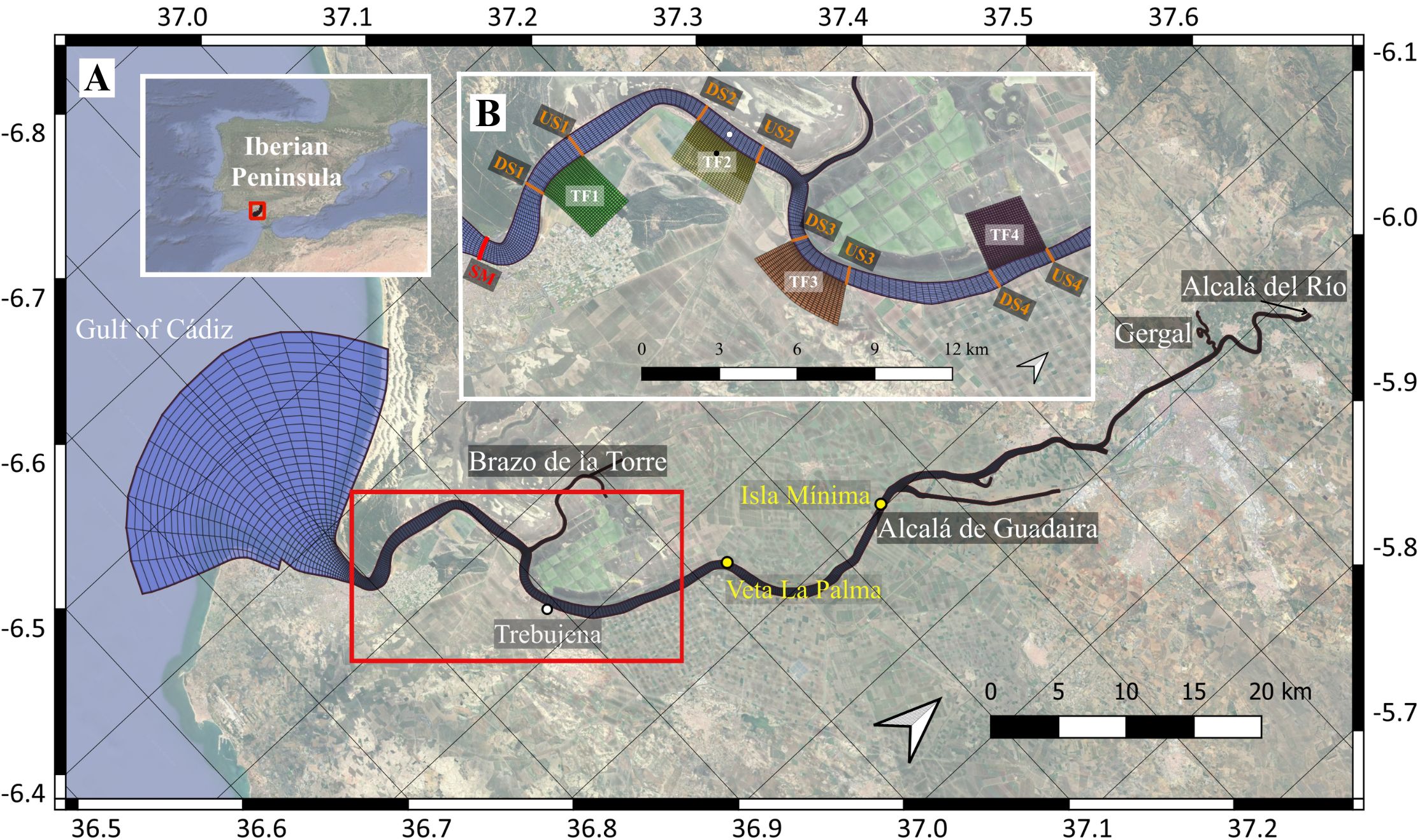
Figure 1. (A) Model domain of the GE used in a previous study (Muñoz-López et al., 2024), showing the two stations used for salinity validation (yellow), the main tributaries, and the closed upstream boundary at Alcalá del Río dam. (B) Locations of the four designed tidal flats (TF1, TF2, TF3 and TF4) used in the experiments described in Table 1. The downstream (DSn, n=1 to 4) and upstream (USn, n=1 to 4) cross-sections associated with each tidal flat, as well as the estuary mouth section (SM), are indicated. Black and white dots mark two stations used for plotting numerical results.

A necessary approach to tidal flat restoration is hydrodynamic numerical modeling, which allows different configurations to be designed, their most suitable locations and their impact on the estuarine system to be assessed without direct intervention (Mahavadi et al., 2024). In this regard, Siles-Ajamil et al. (2019) employed a one-dimensional model to simulate an idealized tidal flat in the Guadalquivir estuary, analyzing how variations in its extension and connectivity with the main channel could influence the estuarine dynamics. Their findings indicated that the recovery of marshes in the 20-kilometer stretch upstream of the mouth of the estuary has notable consequences for tidal wave propagation, increasing tidal amplitudes and reducing upstream currents in proportion to the degree of connection of the marsh with the main channel. This increase in tidal amplitudes may yield a turbidity regime shift that could affect water quality in the estuary, including deteriorated light and oxygen conditions, as was already pointed out by previous studies (Ruiz et al., 2013, 2017). Although their study did not account for nonlinear effects, it provided a valuable initial framework for modeling tidal flats in the Guadalquivir estuary. Building on this work, the current study employs a three-dimensional numerical model recently developed by Muñoz-López et al. (2024) to advance our understanding of tidal flat dynamics in the Guadalquivir estuary. Specifically, this study aims to explore the potential effects of hypothetical tidal flats with varying morphologies and locations on the estuary. By addressing how these tidal flats influence hydrodynamics and salinity patterns, the research provides insights that can guide restoration planning and inform more realistic, site-specific management strategies.

The paper is structured as follows: Section 2 presents and validates the numerical model, with a particular focus on salinity distribution. A hindcast of the year 2021, incorporating all realistic driving forces, has been conducted to calibrate the model and validate its applicability to the highly simplified cases, addressed in subsequent sections. Section 3 outlines the methodology for these case studies, including the configuration of the modeled tidal flats and the experimental setup. Section 4 analyzes the changes induced by a specific tidal flat, while Sections 5 and 6 examine the sensitivity of these changes to different tidal flat locations and morphologies. Finally, Section 7 discusses the findings, highlighting the main conclusions and limitations of the study.

1.1 Study area

The Guadalquivir estuary (GE, hereinafter), located in the southwest of the Iberian Peninsula (Figure 1A), is a relevant and anthropogenized coastal system within the Gulf of Cádiz. It extends approximately 100 km upstream from the river’s mouth to the Alcalá del Río dam. The estuary’s width varies markedly, ranging from approximately 1 km at the mouth to ~100 m at the head. The channel has an average depth of ~6.5 m (Donázar-Aramendía et al., 2018). The river discharge is low, around 25 m³/s on average, being less than 40 m³/s for over 75% of the time, although it can rise to thousands of m³/s during sporadic river flood events (Bermúdez et al., 2021). The regulation of these discharges is essentially conducted by humans in response to their need for water supply and it is well organized and monitored by the automatic database of hydrological information for river flood management (SAIH hereinafter, https://www.chguadalquivir.es/saih). Except for these unusual extreme events, the primary driving force of GE dynamics is the oceanic tide at the mouth, which has mesotidal range and semidiurnal nature, with the M₂ being the most important constituent (Álvarez et al., 2001; Díez-Minguito et al., 2012; Muñoz-López et al., 2024). During low river flows, the estuary is weakly stratified, and salinity decreases from the ocean towards the head of the estuary (Díez-Minguito et al., 2013).

2 Numerical model

2.1 Model configuration

The numerical model is the one employed in Muñoz-López et al. (2024) to whom the reader is referred for a detailed description. Nevertheless, a summary of the main characteristics is given next. The model is the Delft3D-Flow package, a finite difference model for coastal, riverine and estuarine areas developed by WL-Delft Hydraulics. It is employed in its baroclinic version that represents the transport of salinity by a conservative advection-diffusion transport equation in three coordinate directions (Deltares, 2022). The model domain is discretized by a curvilinear orthogonal grid of non-uniform resolution that follows the staggered Arakawa-C grid scheme and extends from 5° 58′ W to 6° 34′ W and from 36° 39′ N to 37° 31’ N (Figure 1A). It uses a vertical sigma-coordinate system of ten levels. Horizontal resolution varies from ~300 m in the open ocean to a few meters in the tributaries.

The model boundary conditions that drive the dynamics of the estuary are: (i) astronomical tides, prescribed at the ocean boundary through the harmonic constants of the selected set of constituents used in Muñoz-López et al. (2024); (ii) freshwater discharges from the SAIH, implemented as water flux conditions in cells adjacent to freshwater sources. Nearly 80% of freshwater discharges come from Alcalá del Río dam (Bermúdez et al., 2021), with secondary inputs from tributaries, namely Brazo de la Torre (average discharge: 0.35 m³/s), Alcalá de Guadaira (0.75 m³/s), and Gergal (0.8 m³/s) (see Figure 1A for locations); (iii) temperature, with a constant value of 19°C at all boundaries, and salinity, with a constant value of 36.7 g/kg imposed at the estuary mouth and 0.1 g/kg for all freshwater discharges; and (iv) atmospheric and radiative forcing at the free surface through the “absolute flux, net solar radiation” scheme (Deltares, 2022), which requires data on relative air humidity, air temperature, and the sum of net solar (shortwave) and atmospheric (longwave) radiation. Wind stress is also prescribed at the open surface boundary. Atmospheric variables are retrieved from the HARMONIE-AROME model of the Spanish State Meteorological Agency (Calvo et al., 2018) and subsequently interpolated onto the spatial grid.

2.1.1 Experimental data

The hydrodynamic datasets, used for calibration and validated with independent observations, are the same as those used in Muñoz-López et al. (2024), where a detailed description is provided. The observations used for validation include water-level records from nine tide gauges, which provide good coverage of the GE, velocity profiles collected at a single point located in the middle stretch of the estuary, and conductivity and water temperature from SAIH at Veta La Palma and Isla Mínima (see locations in Figure 1A). SAIH observations from 2020 to the present are freely available in real-time. Salinity datasets are derived from conductivity and water temperature observations using the thermodynamic equation for seawater (https://www.teos-10.org/) and, in this case, the same datasets are used for both calibration and validation.

2.1.2 Hydrodynamic validation

The hydrodynamic validation methodology follows that of Muñoz-López et al. (2024) and is briefly summarized here for completeness. Harmonic constants derived from water level observations were compared with those obtained from the model via harmonic analysis. The comparison shows that the amplitude differences for the principal M₂ constituent remain below 3 cm throughout the estuary, and phase differences do not exceed 10 minutes (see Figure 2 in Muñoz-López et al., 2024). Time series of observed and modeled water levels at two representative stations located in the lower and upper stretches of the GE (see Figure 1, Muñoz-López et al., 2024) also show very good agreement, with Pearson correlation coefficients of 0.981 and 0.985, and a root mean square errors (RMSE) of 1.3 cm and 1.1 cm, respectively. Velocity profiles recorded in the middle stretch of the estuary and model outputs at the same location show similarly good agreement, with RMSE values below 5 cm/s (see Figure 3 in Muñoz-López et al., 2024). The reader is referred to this work for a more detailed assessment of model performance.

Figure 2

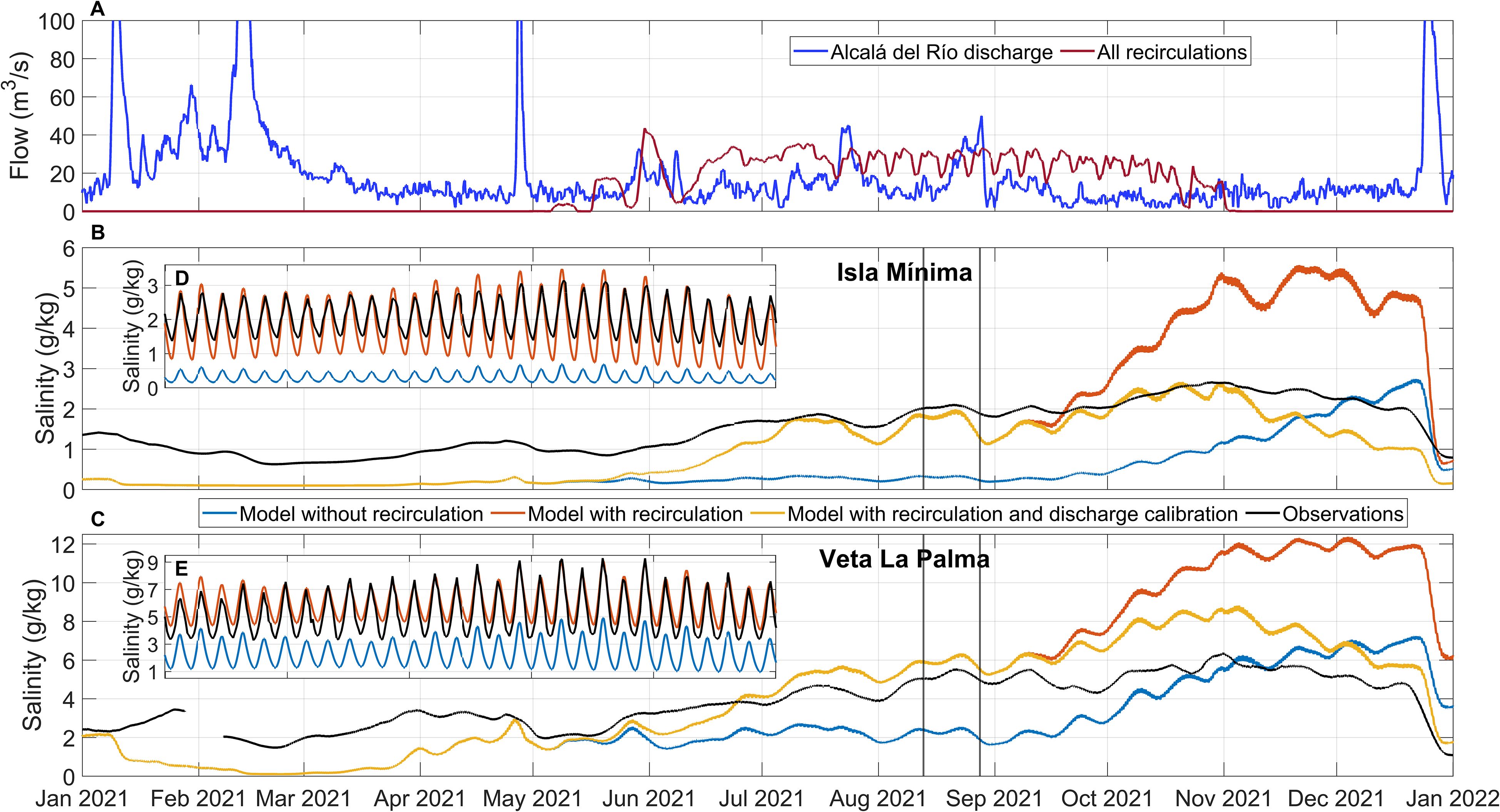
Figure 2. (A) Discharges at Alcalá del Río (light blue) and flows extracted for rice fields irrigation (red) during 2021, smoothed with a 24-hour moving average. The Y-axis is truncated at 100 m³/s to preserve scale readability (this threshold is exceeded four times during the year). (B, C) show the low-passed filtered salinity observations (black line) at Isla Mínima and Veta La Palma stations, along with modeled values under different approaches: blue line excludes the recirculation scheme, whereas the orange and yellow lines include it. The yellow line also includes an additional discharge of 5 m³/s from September 10 to the end of the year (see text for details). Prior to May, the yellow line overlaps the blue and orange, and the orange line is overlapped by the yellow one before September 10. Insets (D, E) display a 15-day segment of the time series indicated by the vertical lines in (B, C), highlighting the good performance of the model at tidal scale.

Figure 3

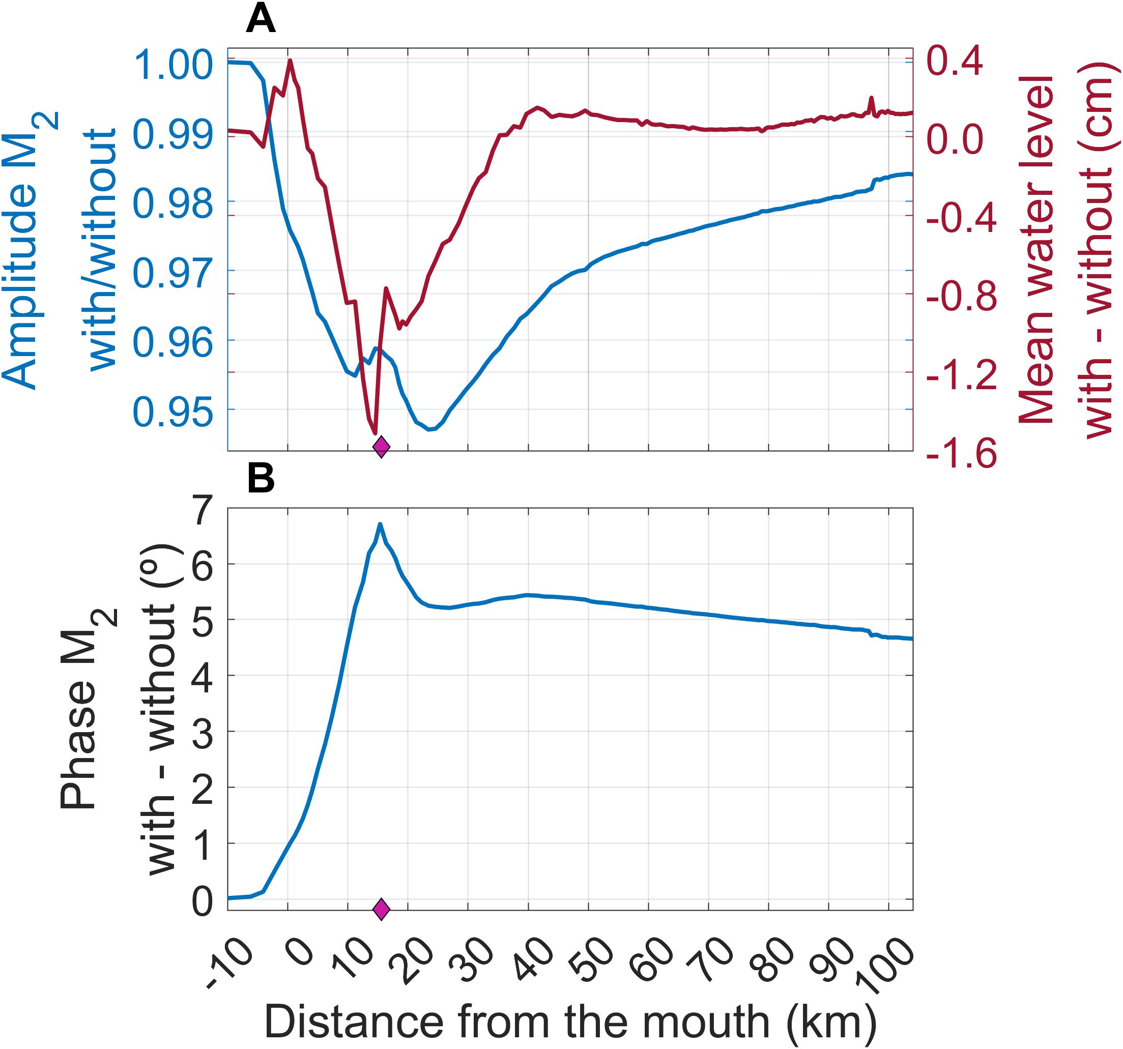
Figure 3. (A) Along-channel ratio of M₂ tidal amplitude of the water level with and without the tidal flat (blue line) and mean water level differences computed as water level with tidal flat minus the reference case. (B) Phase difference of M₂ (with−without) for water level. In both panels, the location of the tidal flat inlet is indicated by the diamond.

2.1.3 Salinity validation

Using a 1D numerical model, Siles-Ajamil et al. (2019) suggested that tidal flats in the GE influence salinity distribution when they are coupled to the main channel through a relatively wide inlets (i.e., wider than ∼100 m). The topic is revisited here using the more sophisticated 3D model described above. The year 2021 was selected as a representative period for model validation and for evaluating the model’s ability to reproduce the observed salinity variability across the estuary, based on the availability of observational data.

The blue line in Figures 2B, C (which is hidden by the yellow line before May 2021) shows that the model slightly underestimates the observed salinity until May-June. This line represents the model’s output without manipulation of the freshwater inputs to the estuary, an aspect that needs to be revisited in the light the following observations: from May to September, observations show a steady increase in salinity that is not captured by the model, which fluctuates around a moderately constant value. From September onwards, the modeled salinity presents a clear increasing trend that is not reflected in the observations, which show a much weaker trend, if any. At the end of the year, a large freshwater discharge of about 200 m³/s brings the two salinity series ​​closer together, demonstrating the good response of the model to such events. At the tidal scale (Figures 2D, E) the model accurately reproduces the timing of the cycle, but neither the amplitude nor the “mean” value, which is lower, as explained above. A likely cause of the discrepancies between model and observations during the late spring to early autumn period, when the datasets diverge the most at both tidal and low-frequency (i.e., seasonal) scales, could be the use of freshwater for rice irrigation, which is not incorporated into the model.

2.1.3.1 Freshwater use for irrigation

During the summer months, rainfall is virtually nil in the Guadalquivir basin, yet reservoirs maintain a minimum ecological flow (Yeste et al., 2018; Romero-Jiménez et al., 2022). In the GE, the ecological flow is increased between May and November for the irrigation of rice fields, which requires a permanent freshwater sheet 20 cm thick to maintain optimal oxygenation, temperature and salinity levels throughout the growth and maturation stages of the rice (Moral Ituarte, 1993). Despite the increase in freshwater discharges, the salinity in the GE does not decrease, but rather increases (black line in Figures 2B, C). The reason is the extraction of fresh or slightly saline water for irrigation upstream the observation stations, monitored by the SAIH (orange line in Figure 2A). This removed water is subsequently returned to the estuary further downstream in smaller (around ¾ of the water intakes) and saltier amounts. The salinity increase is due to evaporation in the flooded rice fields and is estimated in ∼1.5 g/kg. The whole process of water uptake and return is incorporated into the model making use of 16 intake and 18 outflow locations available in the SAIH database (more details in Supplementary Material). The procedure reasonably captures the observed salinity increase between May and September mentioned above (orange line in Figures 2B, C, which is hidden by the yellow one before September 10^th), thus partially reducing the mismatch between model and observations, although notable discrepancies still remain.

2.1.3.2 Discharges recalibration

A weak point of the SAIH data in Figure 2A is that the total flow extracted from the river for rice cultivation is greater than that released by the dam on numerous occasions, implying the uptake of salty water to keep the water balance. This is incompatible with the needs for rice cultivation, which has a clear salinity limit for the water that floods the rice fields. This suggests the existence of additional unregulated inputs that are difficult to quantify and that are not being considered. To fix the issue, a trial-and-error procedure has been carried out to re-evaluate the freshwater discharges to GE, with the aim of adjusting the salinity predictions of the model and the observations. The best matching is obtained when, additionally to the implementation of the recirculation scheme explained in the previous section, a fictitious discharge of 5 m³/s is added to the values provided by the SAIH for Alcalá del Río dam from September 10 onwards (yellow lines in Figures 2B, C). The adjustment has no effect on the water level harmonic constants, that are quite well represented by the model but substantially improves the salinity hindcast (Figures 2D, E), with RMSE of 0.54 g/kg at Isla Mínima and 1.17 g/kg at Veta La Palma stations in summer, the most human-altered season. These satisfactory results support the use of the numerical model to investigate the behavior of salinity in the estuary.

The present work focuses on the response of the estuary under the morphological changes arising from the implementation of future hypothetical tidal flats. To identify concomitant changes in the estuary dynamics and ensure that they are uniquely caused by those morphological modifications, the approach followed in this study is to maintain constant all non-predictable forcings (i.e. freshwater discharges, which in turn would lead to ignoring the strategy of freshwater use and the further adjustment of discharges discussed in the previous sections) and boundary conditions for temperature and salinity, and force the model with the predictable astronomical tide prescribed at the estuary’s mouth uniquely. Furthermore, no atmospheric forcings are imposed. The successfully achieved validation task explained above supports the use of the numerical model to assess the hydrodynamic and hydrographic (i.e. salinity distribution) changes driven exclusively by the implementation of the tidal flats.

3 Methodology

3.1 Tidal flats configuration and experiments

The proposed restoration area is in the lower stretch of the estuary, which is the most morphologically and technically feasible zone for marsh recovery. Four locations were selected (Figure 1B). In each of them, two rectangular tidal flats with different areas (one twice the size of the other) and connection lengths with the main channel were virtually implemented. The connection length (inlet henceforth) refers to the horizontal distance of the inlet that connects the tidal flat to the main channel. Table 1 summarizes the characteristics of the tidal flats.

Table 1

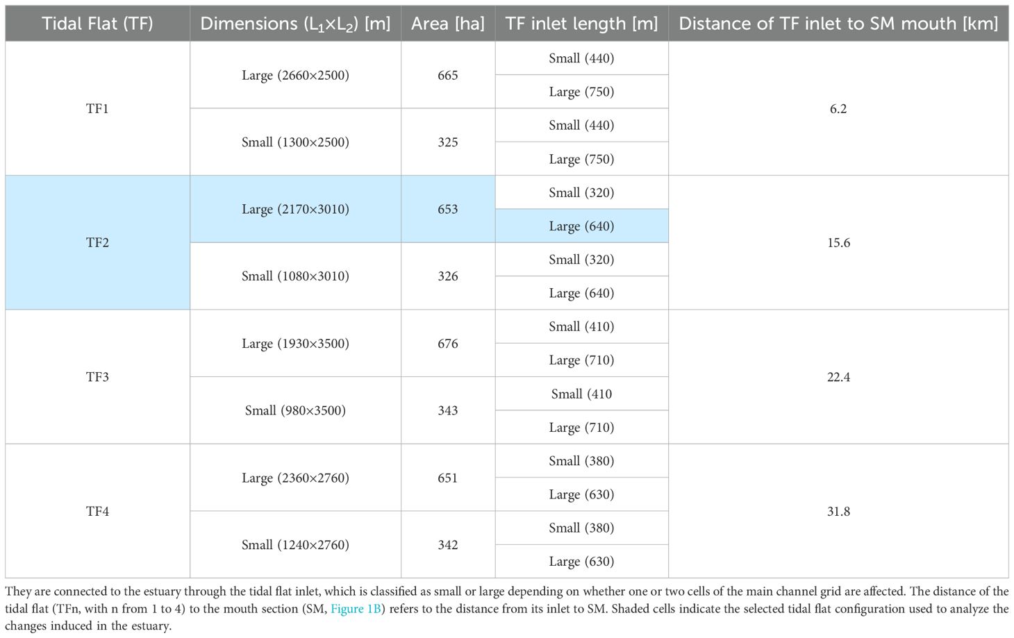
Table 1. Characteristics of the implemented tidal flats.

The tidal flat bathymetry was set to four constant depths: -1, -0.5, 0, and +0.5 m. Its edges correspond to the main channel edges at 2 m. The tidal flat-estuary inlet is deeper, around -1.5 m, and its shape has been smoothed to facilitate water exchange. The shallower bathymetries produce dry cells systematically. A cell is considered dry when the water thickness falls below 2.5 cm.

A total of 64 experiments (4 sites × 2 areas × 2 inlets × 4 bathymetries) were carried out, forced with astronomical tide at the estuary’s mouth uniquely and compared with a reference experiment with no tidal flats. All of them last 7 months, although the first month is not considered to account for the spin-up of the model. Initial conditions in the estuary come from the average of a 6-month simulation and are spatially variable. In contrast, initial conditions in the tidal flats are constant and equal to the initial value of the estuary at the tidal flat location. Constant discharges of 25 m³/s (Alcalá del Río), 0.35 m³/s (Brazo de la Torre), 0.75 m³/s (Guadaira) and 0.8 m³/s (Gergal), all of them with salinity 0.1 g/kg and temperature 19 °C, are imposed in the inland boundaries and constant salinity of 36.7 g/kg and temperature 19 °C are imposed at the GE mouth.

3.2 Analysis of numerical data

The modeled water level, salinity, and along-channel velocity were extracted at 153 evenly spaced points along the estuary to generate along-channel plots of these variables. Volume transport was computed at the mouth of the tidal flats, as well as in the sections upstream and downstream of them, as shown in Figure 1B. Differences between simulations with and without tidal flats were calculated for all the variables.

Two sets of experiments were conducted. The first one analyzed how different morphological configurations of a tidal flat affect the estuary, varying its area (326 and 653 ha), inlet length (320 and 640 m), and bathymetry (-1, ± 0.5, and 0 m). The second set examined the effect of tidal flat location within the estuary. To this aim, similar configurations for the tidal flats were selected, leaving the location as the unique variable of the study.

4 The impact of a tidal flat on the estuary

A tidal flat connected to an estuary is an ecosystem that floods and drains according to the tidal cycles of the estuary: it fills during the rising tide and empties during the falling tide. It exchanges water with the estuary through its inlet, which is expected to be saltier on average than the water that would exist in the same part of the estuary without the tidal flat. This occurs because it fills with saltier water carried by tidal currents from the ocean during the rising tide. As a result, it acts not only as a water reservoir but also as a salt reservoir, thereby modifying the estuary’s properties. This behavior is independent of the specific morphology of the implemented tidal flat; therefore, the changes induced by a specific tidal flat are first analyzed in the following section, and subsequently we discuss the sensitivity of these changes to the different locations and morphologies defined in Table 1. The tidal flat selected for detailed analysis corresponds to tidal flat TF2 in its most extreme configuration—largest area and inlet (see shaded cells in Table 1), and greatest depth (bathymetry of -1 m)—and is located 15.6 km upstream (Figure 1B). This specific case was selected as it represents the most significant potential alteration in the estuary’s hydrodynamics and salinity distribution, thus providing a good example of the tidal flat’s impact, while its intermediate location ensures a representative assessment of the tidal flat’s influence within the system.

4.1 Tidal wave changes

A tidal flat causes detectable changes in the tidal wave propagation in the estuary. A first consequence is the increase in tidal transport (tidal prism) through the mouth of the estuary (section SM, Figure 1B) because the surface area of the estuary has now been enlarged. For the analyzed TF2 configuration, the amplitude of M₂ constituent of water transport through SM increases by 9.4% compared to the situation without tidal flat. The capture of water by the tidal flat makes the amplitude of the M₂ water level oscillation diminish throughout the whole estuary (Figure 3A). The decrease is greater in the vicinity of the tidal flat inlet, where the amplitude is 95% of the value in the reference situation. The M₂ phase difference increases steadily from the mouth of the GE to the location of the tidal flat (Figure 3B), indicating a delay in wave propagation, resulting in a few minutes longer transit time between the two sites. The difference reaches a maximum at the location of the tidal flat and becomes almost constant upstream, showing only a very slight decrease. Despite this stabilization, the transit time along the entire estuary remains longer with a tidal flat than without it. Dynamically, the effect of the tidal flat is similar to an increase in friction in the estuary, which also decreases the amplitude and phase velocity of the wave (Muñoz-López et al., 2024). The mean water level in the estuary also shows a slight decrease near the tidal flat that reaches ∼1.5 cm at the tidal flat inlet (red line, Figure 3A). Further upstream, changes are negligible.

4.2 Salinity changes

Figure 4A shows that the mean salinity in the estuary increases with the presence of the tidal flat and it does it more noticeably in the vicinity of the tidal flat location. In fact, the peak salinity increase is attained a short distance upstream of the tidal flat inlet, as shown in Figure 4B. This figure allows for the definition of a region of tidal flat influence, which is defined as the portion of the estuary where the mean salinity with the tidal flat exceeds the salinity of the reference situation by a given amount ΔS₀. In this study, ΔS₀ = 1 g/kg has been assumed (dash black line, Figure 4B) and the region of tidal flat influence covers ∼33 km, from slightly before km 5 to slightly after km 35 from SM, extending to both sides of the tidal flat asymmetrically, reaching further upstream.

Figure 4

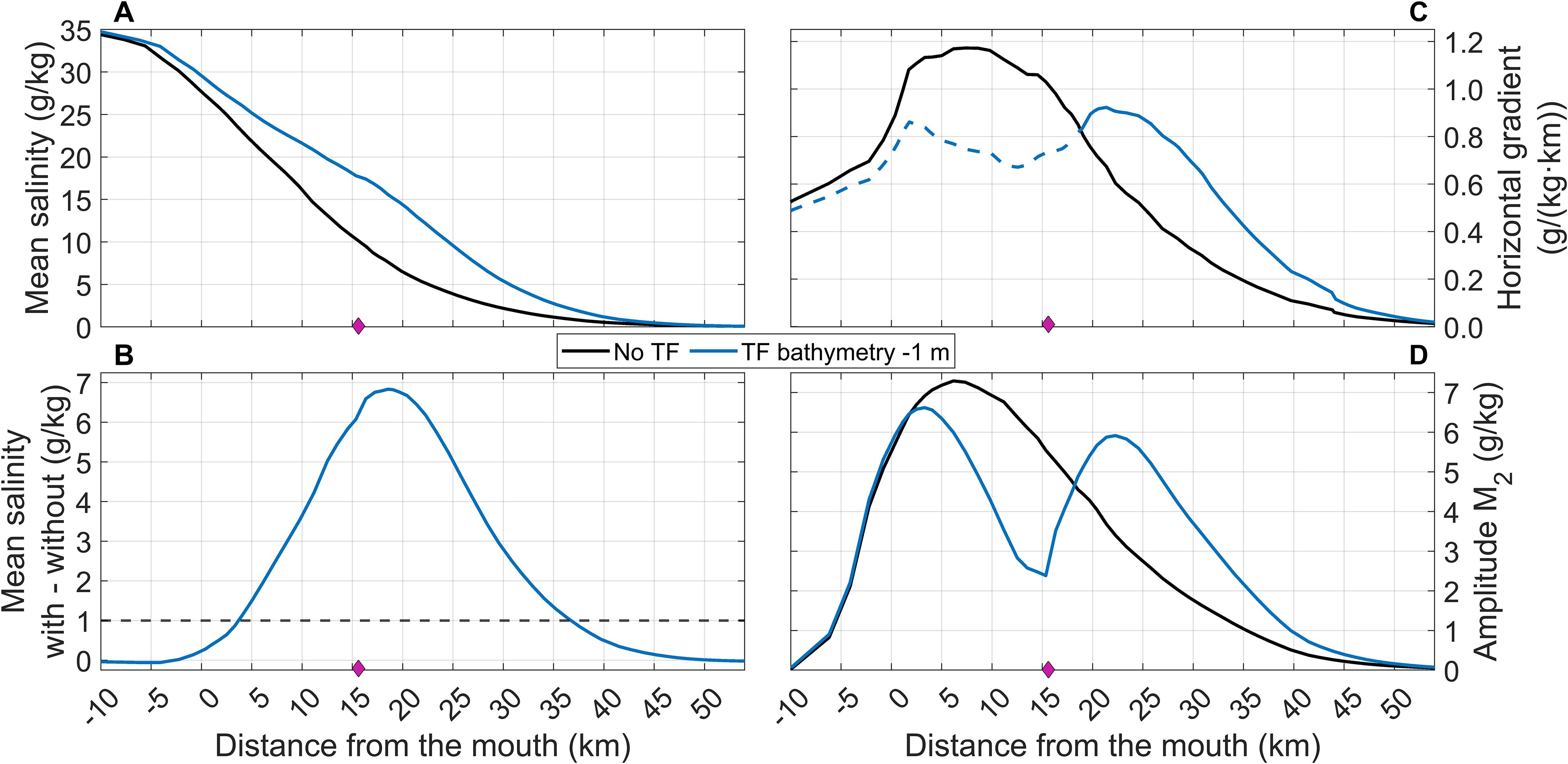
Figure 4. (A) Along-channel profiles of the mean salinity for the reference situation with tidal flat (blue line) and without it (black line). (B) Differences in mean salinity, computed as the situation with TF2 minus the reference. (C) Mean salinity horizontal gradient. (D) M₂ amplitude of salinity. The horizontal dashed line in panel (B) represents the ΔS₀ = 1 g/kg salinity difference used to define the region of influence of the tidal flat (see text). Solid and dashed blue lines in panel (C) indicate the regions where the horizontal gradient is greater and smaller, respectively, with the tidal flat than without it. The diamond marks the location of the tidal flat inlet.

The tidal flat reduces (dashed lines, Figure 4C) the salinity gradient downstream and increases (full lines, Figure 4C) it upstream of its location, which causes a concomitant decrease and increase in the tidal amplitude of salinity (Figure 4D). The tidal amplitude reduction is particularly noticeable near the tidal flat inlet (Figure 4D). Since salinity patterns are primarily due to salinity advection, it is convenient to briefly describe the water exchange between the estuary and the tidal flat.

4.2.1 Exchange of water estuary – tidal flat

Figure 5 illustrates the main features of the water exchange between the tidal flat and the estuary, which is driven by the water level difference between both systems. Around high water the flow across the inlet is zero as the water level in the tidal flat and the estuary are the same (see red arrows in Figure 5). When the falling tide starts, it does slightly earlier in the estuary and the tidal flat begins to empty (negative flow, green dashed line, in Figure 5). As the downstream flow in the estuary increases during ebb tide, the tidal flat empties faster and faster until it reaches a maximum negative flow across the inlet. As the water level in the tidal flat drops and the thickness of the water sheet decreases, friction becomes more important and controls the flow towards the estuary, which declines progressively. Before the water level in the tidal flat reaches the bottom (i.e., before it dries completely), the next rising tide arrives at the tidal flat entrance, marking the beginning of the positive flow (red dot in Figure 5), and the tidal flat starts to refill. This flow increases rapidly due to a faster rise of the tide in the estuary than in the tidal flat, causing a water level gradient towards the latter. The solid and dashed blue lines in Figure 5 illustrate this situation. As the high-water approaches, both blue lines come closer together, and the gradient —and, consequently, the positive flow— progressively decreases after reaching a peak. Refilling continues at a slower rate until high water, at which point the flow stops and a new cycle begins.

Figure 5

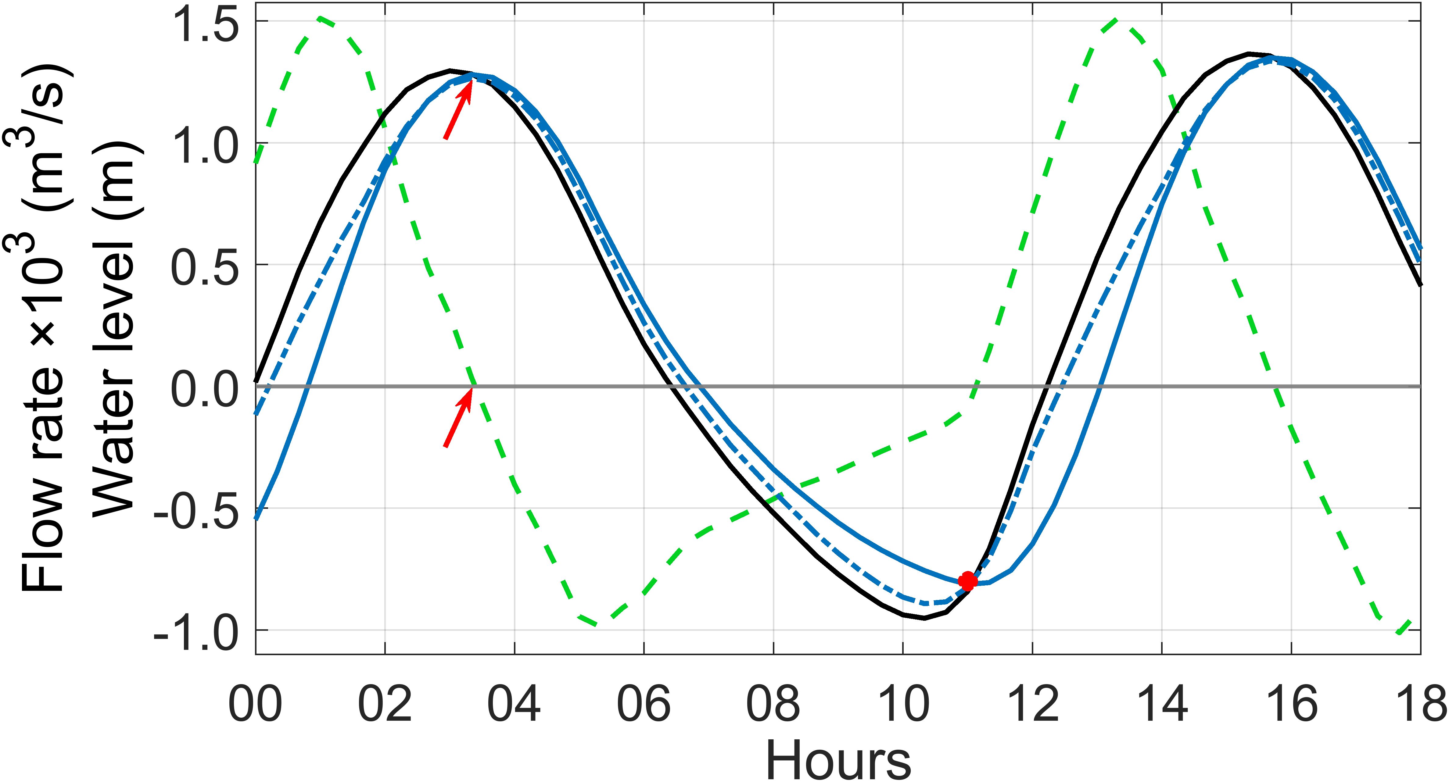
Figure 5. Flow (dashed green line) across the inlet of the tidal flat and water level near the center of it (solid blue line; see black dot in Figure 1B) and at a point in the estuary in front of its inlet (see white dot in Figure 1B) for the reference case without tidal flat (black line) and with the tidal flat (dot-dashed blue line). Positive values indicate flow from the estuary into the tidal flat and negative values represent flow from the tidal flat into the estuary. Red arrows mark the moment when the filled tidal flat starts to drain. The red dot marks the moment when the tidal flat starts to refill.

4.2.2 The tidal salinity cycle

Solid and dashed black lines in Figure 6A show the time evolution of the surface salinity at a point in the estuary, just in front of TF2 (white dot in Figure 1B or black dots in Figures 6B–G), in the cases with and without the tidal flat, respectively. Six moments of special interest (vertical lines B to G), are highlighted in the series. The time-averaged salinity is clearly larger in presence of the tidal flat and its range of fluctuation is clearly smaller. The solid pink line represents the salinity at the center of the tidal flat, which is always lower than at the estuary, except for a brief period around low tide (time C in Figure 6A). Its range of variation is also smaller than in the estuary and remains fairly constant most of the time. The point of interest here is the distorted profile of salinity in the estuary observed around high tide (solid line around time E in Figure 6A), which attains a minimum shortly after high water (see inset in Figure 6E). This contrasts with the maximum found in the absence of tidal flat (dashed black line), which is the expected result, since salinity must increase as long as the flood continues.

Figure 6

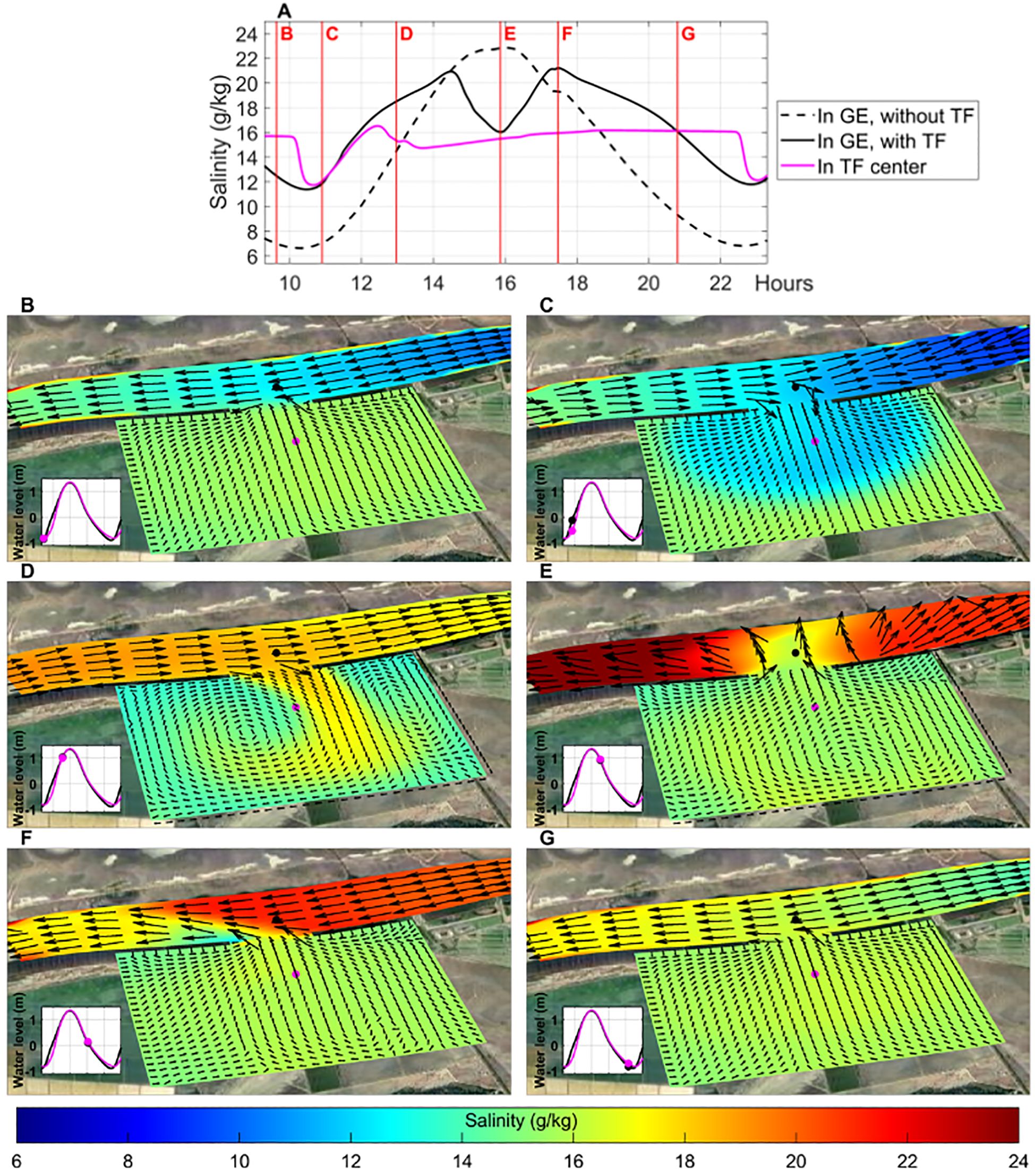
Figure 6. (A) Solid pink line: surface salinity near the center of the tidal flat (see black dot in Figure 1B or pink dots in (B–G). Solid and dashed black lines: same at a point in the estuary in front of the tidal flat inlet (see white dot in Figure 1B or black dots in (B–G) in the presence and absence of the tidal flat, respectively (see legend). Labeled vertical red lines refer to the time in which the salinity (color scale) and velocity (arrows) fields are depicted in the snapshots in (B–G). Insets in these panels illustrate the moment of the tidal cycle corresponding to each snapshot.

In order to explain this pattern, snapshots of the velocity and surface salinity fields at the six selected moments of the tidal cycle are represented in Figures 6B–G. Around low tide, the water in the tidal flat is saltier than that of the estuary (Figure 6B; time B in Figure 6A). This is the only moment when this occurs. When the flood tide begins, the tidal flat fills with water that is less saline than the water inside (Figure 6C; time C in Figure 6A). Shortly after, the water coming from the ocean begins to flood the tidal flat that is already saltier (Figure 6D; time D in Figure 6A), and the salinity of the tidal flat increases until it reaches a rather constant value. It continues increasing in the estuary until the salinity curve shifts from rising to falling. The reason is the flow through the inlet of the tidal flat, which has reversed near the high tide, as explained above, and now moves toward the estuary, carrying fresher water (Figure 6E; time E in Figure 6A). At this moment, the water upstream of the tidal flat is saltier than the water exiting the tidal flat but still moves landward. When the tidal flow upstream reverses, this saltier water flows in front of the tidal flat again (Figure 6F; time F in Figure 6A), increasing the salinity, which attains the second maximum shown in Figure 6A. Afterward, the salinity in the estuary gradually decreases, completing the cycle. The salinity in the tidal flat remains fairly constant until the new cycle brings in fresher water (Figure 6B). In some sense, the tidal flat acts as a salinity reservoir, storing waters that are, on average, saltier than those found in the estuary without the tidal flat, and whose exchange with the estuary creates the region of tidal flat influence defined earlier.

The resulting two-maximum pattern is responsible for the notable reduction of the horizontal salinity gradient in Figure 4C around and downstream of the tidal flat compared to the reference situation. As we approach the upstream limit of the region of tidal flat influence (Figure 4B), the horizontal salinity gradient exceeds that of the reference situation (Figure 4C), since salinity decreases more rapidly because of the intrusion of fresher riverine water entering after the previous low tide (Figure 4A). Since local salinity changes are driven by tidal advection, this pattern reduces salinity fluctuations downstream of the tidal flat and increases them upstream (Figure 4D). It is as though the presence of the tidal flat homogenizes the estuary’s salinity field in its vicinity, causing tidal salinity fluctuations to be largely reduced there.

5 Influence of tidal flat morphology

The influence of different morphological configurations of a tidal flat on the GE is analyzed in this section, based on the first set of experiments (see Section 3.2). Again, TF2 has been selected as the case study. The experiments conducted at the other locations yield similar results. The configurations include large and small areas (323 and 653 ha), long and short tidal flat inlets (320 and 640 m), and four bathymetries (-1 m, -0.5 m, 0 m and +0.5 m). Experiments with tidal flats featuring a bathymetry of +0.5 m, which are only flooded when the estuary water level exceeds this elevation, result in very small modifications compared to the reference situation and are only discussed occasionally.

5.1 Tidal waves and tidal flows

5.1.1 Water level

The mean water level decreases systematically around the tidal flat, following a pattern similar to the one displayed in Figure 3A. The reduction is greater for deeper tidal flats. Shorter inlets result in smaller modifications in the mean water level compared to longer inlets, while the area of the tidal flat is the least influential parameter. In any case, changes in the mean water level are less than 1.5 cm and therefore negligible (results not shown).

Figure 7 shows the harmonic constants of the water level for the M₂ constituent. For all configurations, tidal amplitude decreases, and the phase increases in the vicinity of the tidal flat location, with changes gradually fading out away from its location. These changes follow the pattern discussed in the previous section. Tidal amplitudes and phases are clearly sensitive to the size of the tidal flat (compare Figures 7A–D, with Figures 7E–H). For a given area and inlet size, deeper bathymetries cause greater differences, while the size of the inlet has a relatively minor effect. Overall, the impact of the modeled tidal flats on the GE water level, compared to the reference situation, is always less than 10%, a value that is only reached under the most extreme configurations (large area, inlet, and depth). Considering all configurations, the average departure from the case without a tidal flat is around 5%.

Figure 7

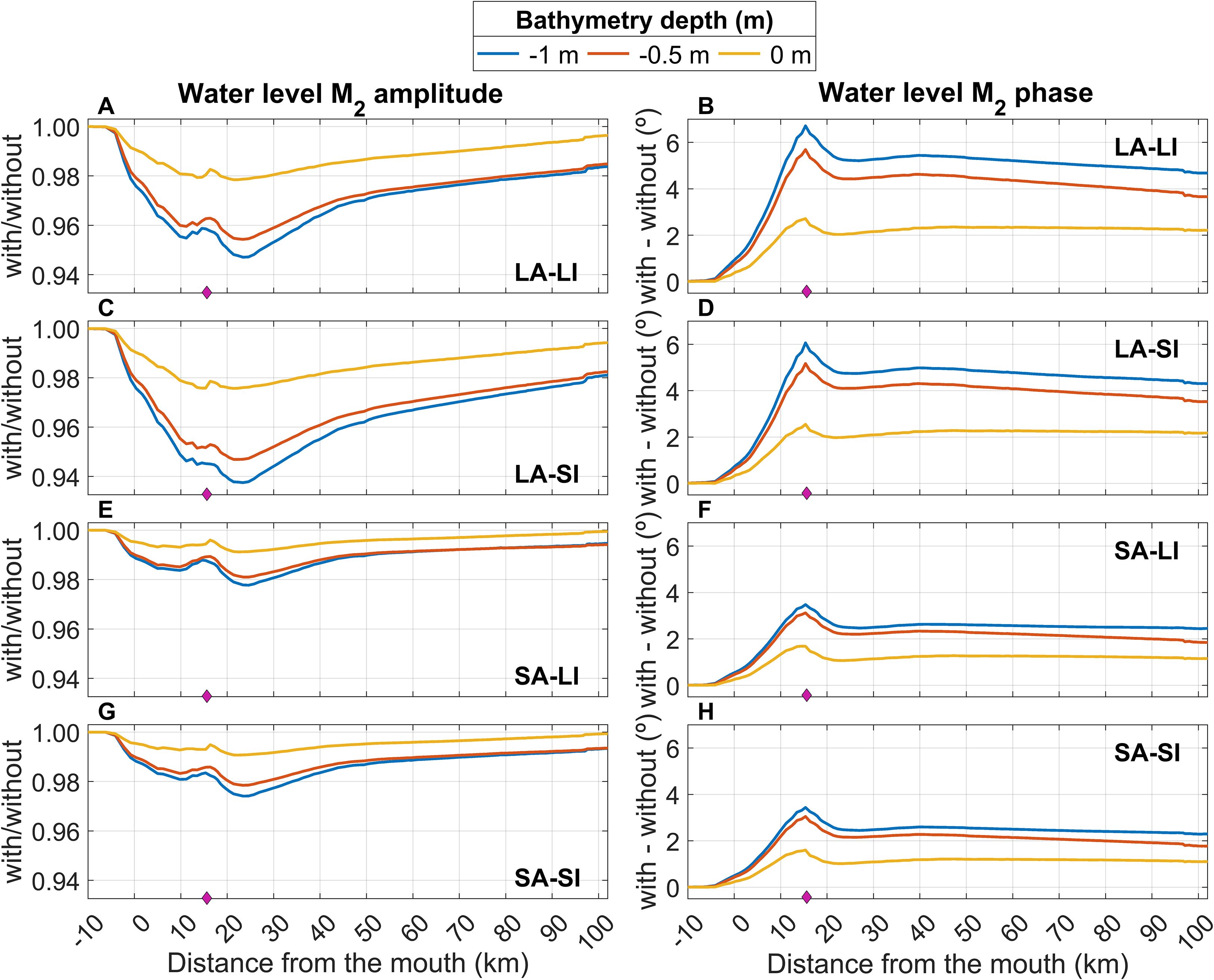
Figure 7. Ratio of amplitudes (A, C, E, G) and phase difference (B, D, F, H) of M₂ harmonic constants of water level along the estuary resulting from the implementation of TF2. The plots show the four area-inlet configurations (LA, large area; SA, small area; LI, large inlet; SI, small inlet) and three bathymetries (see legend). The tidal flat location is marked with a pink diamond.

5.1.2 Tidal flows

Table 2 presents the M₂ harmonic constants of volume transport across the mouth section (SM, Figure 1B) for twelve of the sixteen configurations implemented in TF2 (the +0.5 m bathymetry causes negligible variations and is not included). The amplitude always increases compared to the reference situation, ranging from 9.4% for the most extreme case (largest area, largest inlet, and deepest bathymetry, as discussed in Section 4.1) to 2.4% in the least extreme one (smallest area, smallest inlet, and shallowest bathymetry). For a given tidal flat extension and inlet configuration (shaded blocks, also identified by the letter code in the second column of Table 2), volume transport is relatively sensitive to bathymetry, with an increase approximately twice as large for the -1 m bathymetry compared to the 0 m bathymetry (see Table 2, last column). The phase always increases, but by less than 2° (within the confidence interval) in all cases, and by less than 1° in most of them. These phase changes are so small that they can be neglected and are not analyzed here. From a hydrodynamic perspective, however, this phase increase, even if small, corroborates that tidal flats produce the same effect as an increase in friction within the estuary, as discussed in Section 4.1.

Table 2

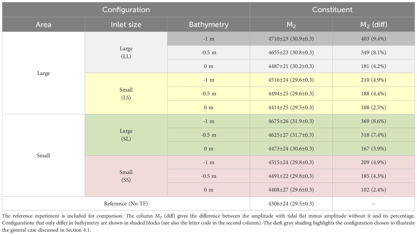
Table 2. Amplitude (m³/s) and phase (degrees, in brackets) of M₂ constituent with their corresponding standard deviations for the volume transport across the SM section (see Figure 1B) for different configurations of TF2.

Regarding the other parameters, the inlet size has a greater influence than the tidal flat area, as evidenced by comparing blocks LL (gray shade) and LS (yellow) in Table 2. For a given area, the volume transport through section SM is between ∼2% and ∼4% higher when the tidal flat’s inlet is large rather than small (compare the gray and yellow blocks for the large area and green and red for the small one). When comparing blocks with the same inlet size but different areas (gray and green blocks on one hand, yellow and red on the other), the variations remain below 0.7% for all bathymetries.

Figure 8 illustrates the water exchange between the estuary and the tidal flat with the largest area and inlet for the four bathymetries considered (+0.5 m included). The general behavior follows the description already provided in Section 4.2.1, where the tidal flat fills and drains in response to the tidal cycle, influenced by friction and water level gradients. The same mechanisms driving the inflow and outflow of the tidal flat apply. However, the inclusion of shallower bathymetries introduces additional nuances, which are discussed next.

Figure 8

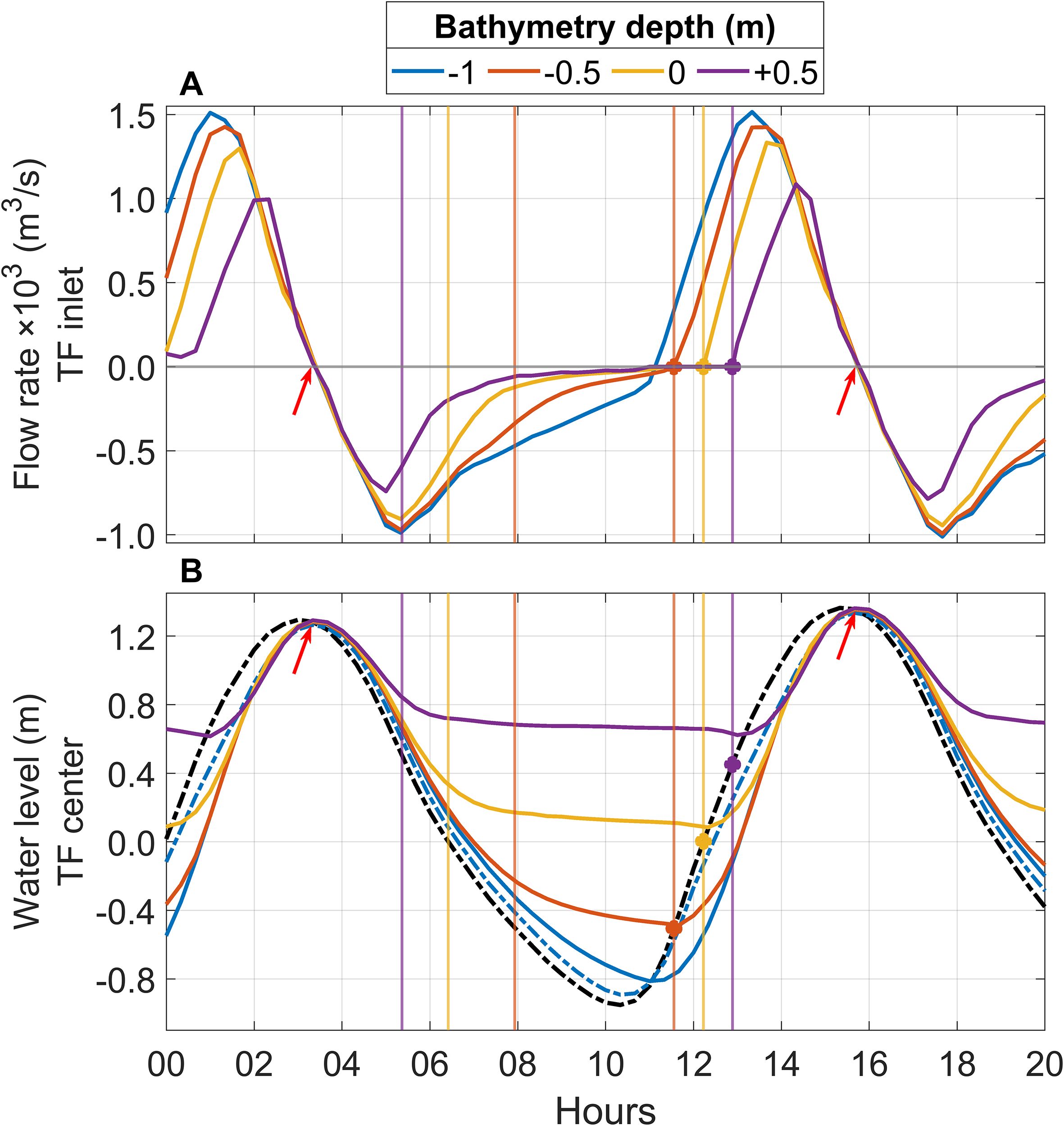
Figure 8. (A) Flow across the TF2 inlet for the largest area and inlet size configuration and the four bathymetries considered (color-code in the legend). Positive values indicate the flow from the estuary into the tidal flat; negative values indicate the opposite. Red arrows mark the moment when the filled tidal flat starts to drain. (B) Water level near the center of the tidal flat (see black dot in Figure 1B) for the four bathymetries (solid lines, same color-code as in (A) and at a point in the estuary in front of the inlet (see white dot in Figure 1B) for the reference case without tidal flat (thick black dashed line) and in the presence of the tidal flat with the deepest bathymetry (-1m, thick blue dashed line). Curves for the other three bathymetries have not been plotted for the sake of clarity, as they are very similar to the dashed blue one. Vertical lines indicate the time at which the water level in the estuary reaches the depth of the different flat bathymetries (same color code). Notice that no such lines exist for the deepest bathymetry. Additionally, colored dots mark these moments during the rising tidal semi-cycle.

The relevant difference arises from the fact that the water level in the estuary eventually falls below the bottom of the tidal flat for all bathymetries except -1 m (vertical lines in Figure 8A). In such cases, friction increasingly controls the drainage of the tidal flat as the water table thins, to the point of preventing complete drying. This is illustrated in Figure 8B, which shows that during periods when the tidal flat is expected to be dry (i.e., during the interval between the color-coded vertical lines in Figure 8, when the water level in the estuary is below the tidal flat bottom), it remains partially flooded. Instead of fully drying, it exhibits an asymptotic decrease in water level (Figure 8B), a pattern also reflected in the flow through the inlet (Figure 8A). For the deeper bathymetry (-1 m), where the water level in the estuary stays above the tidal flat bottom (no vertical blue lines in Figure 8), the asymptotic drainage patterns are less prominent, but still detectable, particularly in the inlet flow (blue line, Figure 8A). Friction delays the tidal flat’s low tide, which lags the low-water tide in the estuary: the shallower the bathymetry, the greater the delay and the flatter the asymptotic tail of the water level curve (Figure 8B). A similar pattern applies to the flow through the inlet in Figure 8A.

Additionally, Figure 8 shows that the refilling process depends on bathymetry. It begins when the water level in the estuary rises above the tidal flat bottom (colored dots in Figure 8A), whereas the onset of drainage (negative flow) is identical in all cases (see red arrows), as it only depends on the high tide in the estuary.

The core of this analysis applies to other configurations with different extension and inlet sizes, where the results obtained show only small and irrelevant changes compared to those explained above.

5.2 Salinity

Figure 9 confirms that the mean salinity in the estuary increases with the presence of the tidal flat, regardless of its morphology. The maximum increase is observed approximately 3–4 km upstream of the inlet location, with this distance increasing slightly with the depth of the tidal flat bathymetry. The increase in salinity is directly correlated with the depth of the tidal flat (see the different curves in each panel of Figure 9) and the size of the inlet (compare Figures 9A, B, and Figures 9C, D), but it is relatively insensitive to its area (compare Figures 9A, C, and Figures 9B, D). The highest peak value, close to 7 g/kg, is reached under the most extreme configuration analyzed (deepest, largest area and inlet, Figure 9A). The region of tidal flat influence (defined in Section 4.2), delimited by the dashed black line plotted at 1 g/kg, extends from ∼21 km for the smallest area and inlet with 0 m bathymetry (yellow line in Figure 9D) to ∼33 km for the largest area and inlet with -1 m bathymetry (blue line in Figure 9A). This region does not exist for the +0.5 m bathymetry, which has not been discussed so far, and is solely included in Figure 9 to show that it does not produce significant changes in the estuary, as anticipated.

Figure 9

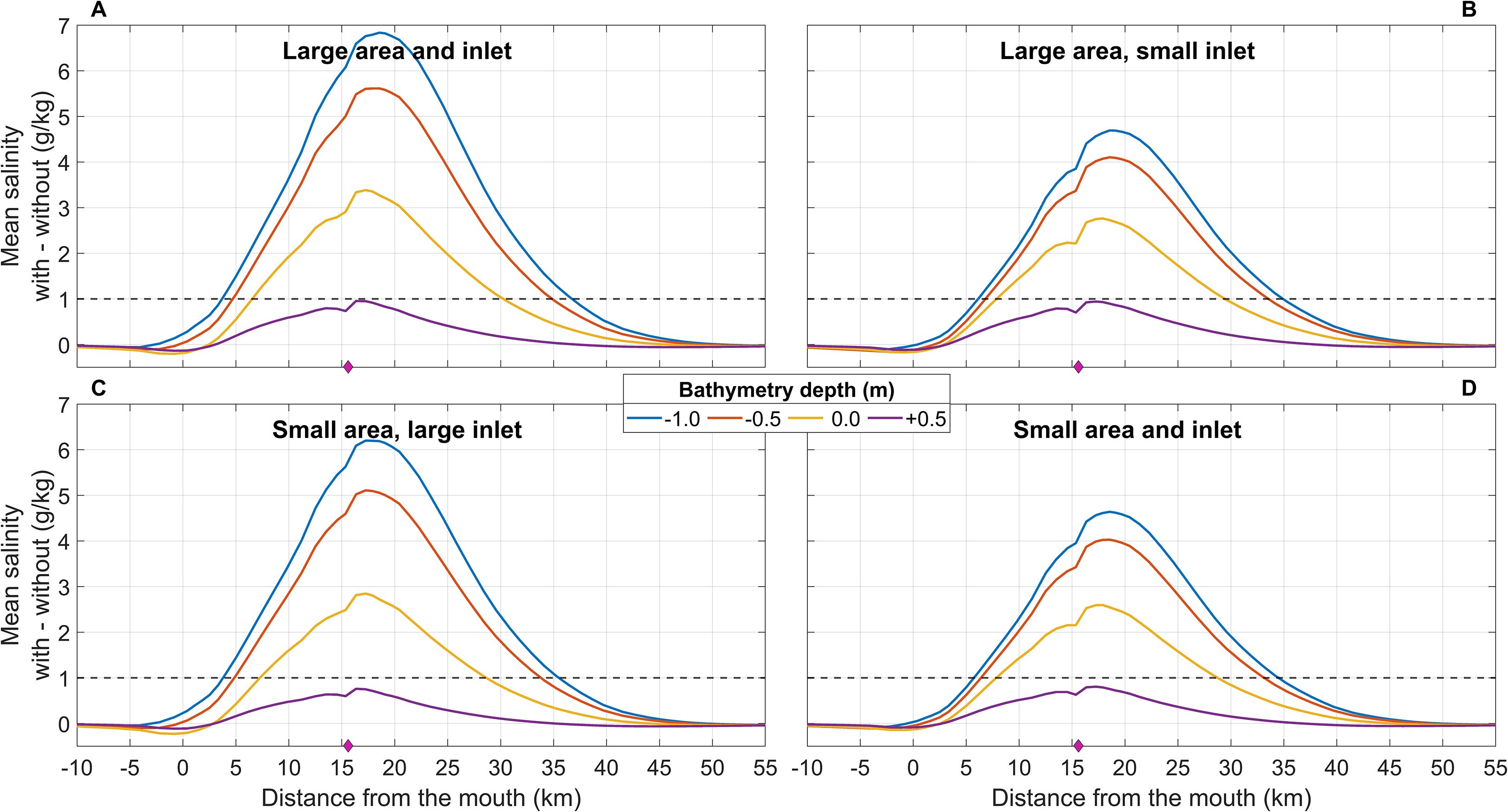
Figure 9. Along-channel profiles of the difference in the mean salinity with tidal flat minus salinity without tidal flat for all the configurations of TF2, including the bathymetry of +0.5 m (see legend). The location of the tidal flat inlet is indicated by the pink diamond. Horizontal dashed lines highlight the 1 g/kg salinity difference used to delimit the region of influence of the tidal flat.

The salinity gradient decreases downstream and increases upstream of the tidal flat, compared to the reference situation. This causes a concomitant decrease and increase, respectively, in the tidal amplitudes of salinity (see Supplementary Figure S2), following the pattern discussed in Section 4.2. The transition from decrease to increase occurs at the same location as the maximum salinity differences shown in Figure 9. As a result, the salinity gradient tends to remain constant around the tidal flat, with a small minimum downstream that is more pronounced for deeper bathymetries and larger inlets (see Supplementary Figure S2).

6 Location of the tidal flat

The sensitivity of the location of a tidal flat in the estuary is addressed in this Section. The analysis must be carried out employing similar morphologies for all the tidal flats. To this end, the selected configuration corresponds to the largest area (~660 ha), the largest inlet (~512 m), and a bathymetry of -0.5 m (see details in Table 1). The section follows the same structure as the previous one.

6.1 Tidal waves and tidal flows

6.1.1 Water level

The mean water level (Figure 10A) decreases to a minimum a short distance downstream of the tidal flat inlet. The closer the tidal flat is to the estuary mouth, the more marked the minimum becomes. Farther downstream, the mean level recovers to the value of the reference situation, whereas upstream, all configurations display a very slight increase compared to this situation. Changes hardly reach 1.5 cm for TF1 (the most downstream location) and can be neglected.

Figure 10

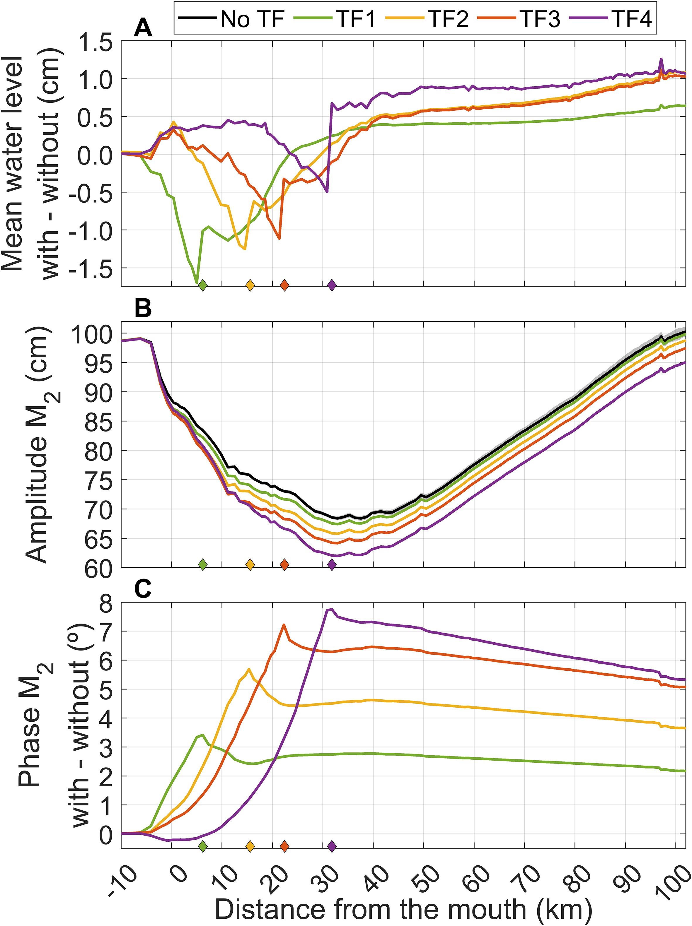
Figure 10. (A) Along-channel mean water level differences computed as the water level with the tidal flat minus the reference case without it for the four analyzed locations (see legend for color code). (B) Profiles of M₂ amplitude, showing the reference case for comparison. (C) Same as (B), but for the M₂ phase difference (tidal flat minus reference case). The location of the tidal flat is indicated by diamonds colored according to the legend.

Tidal flats always reduce the amplitude of the tide (exemplified by the M₂ constituent), regardless of their location (Figure 10B). The reduction mainly occurs downstream of the tidal flat, and the farther upstream the tidal flat is, the greater the changes, which can reach almost 10 cm in the case of TF4. In all cases, upstream the tidal flat inlets, the amplitude maintains the same difference relative to the reference case that was already reached near the tidal flat location. In other words, no additional changes occur upstream of the inlet; only those that have already taken place are maintained. Phases show a monotonic, slight phase increase between the mouth of the estuary and the tidal flat, peaking around the location of the latter (Figure 10C), which in turn implies a slightly longer transit time between the two sites. The farther upstream the tidal flat is, the greater the delay, which can reach ∼18 min (8°) in the case of TF4. Upstream of the tidal flat, no further delay accumulates. On the contrary, it is reduced slightly (negative slope in the curves of Figure 10C), but not enough to compensate for the increase experienced downstream of the tidal flat. The result is longer transit times from the mouth to the head of the estuary. The further upstream the tidal flat is, the longer this time.

Overall, the tidal flats modify the wave progression by reducing the amplitude and increasing the transit time. Both effects occur mainly between the mouth of the estuary and the location of the flat, and they become more notable the farther upstream the tidal flat is located. In all cases, the resulting changes reach a maximum of approximately 10% and, therefore, are of limited relevance.

6.1.2 Tidal flows

Table 3 shows the harmonic constants of volume transport at the SM section (Figure 1B) for the harmonic constants of the M₂ constituent. As mentioned in Section 4, the presence of tidal flats always increases the volume transport through SM: the closer the tidal flat is to SM, the greater the increase (column SM (diff), Table 3). For instance, the amplitude of the M₂ constituent increases by 9.5% in the TF1 case compared to the reference situation, but only by 1.8% in the TF4 case. Similar trends are observed for the remaining constituents (Supplementary Table S1). In contrast, the phase generally increases with the distance from SM, except for the semidiurnal constituents in the TF1 case, which show minimal changes.

Table 3

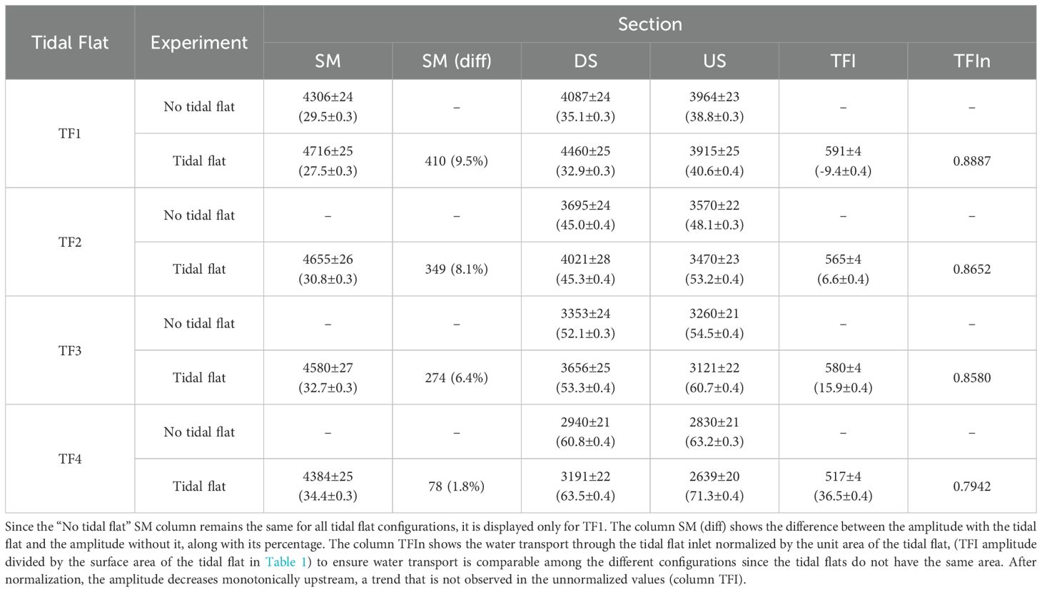
Table 3. Amplitude (m³s^-¹) and phase (degrees, shown in brackets below) of the M₂ constituent with their corresponding standard deviations for water transport across the estuary mouth section (SM; Figure 1B), the downstream (DS) and upstream (US) sections of each tidal flat, and across the tidal flat inlet (TFI) for the second set of experiments, including the reference case for comparison.

Regarding the volume transport at the downstream and upstream sections of each tidal flat (see Figure 1B), the amplitude is always greater downstream (compare columns DS and US, Table 3), which is explained by the different tidal range in both sections when no tidal flat is present, and by the different tidal range plus—primarily—the flow through the tidal flat inlet (column TFI) when it is present. The phase difference between the DS and US sections reflects the time needed for the tidal wave to move from one section to the other. A tidal flat between the two increases the phase difference, meaning the wave takes longer to propagate. As mentioned earlier, the tidal flat can be considered a source of increased friction in the estuary, leading to a reduction in wave amplitude (Figure 10B) and an increase in phase (Figure 10C).

One might hypothesize that the reduction in the increment of water transport through section SM as the tidal flat is located farther from the mouth (column SM (diff), Table 3) could be due to a decrease in water uptake by the tidal flat itself. In fact, column TFIn in Table 3, which shows the M₂ amplitude of water transport across the flat inlets normalized by the tidal flat areas, follows the same pattern as column SM (diff). However, the normalized amplitude (column TFIn, Table 3) does not decrease as significantly as the water transport across section SM (SM (diff)), which refutes the hypothesis. Instead, the explanation lies in the V-shape of the tidal amplitude in the estuary (Figure 10B; see also Muñoz-López et al (2024) for a comprehensive explanation of the origin of this V-shape). The four tidal flats analyzed are spatially arranged in the direction of decreasing tidal amplitude (Figure 10B). The smaller the tidal amplitude at the tidal flat, the smaller the amount of water exchanged with the estuary in each tidal cycle and, consequently, the smaller the required increase in water transport through the SM section.

6.2 Salinity

Figure 11A shows that tidal flats increase the time-averaged salinity throughout the estuary, regardless of their location, with the greatest salinity occurring slightly upstream of the tidal flat inlet (Figure 11B). Regions of tidal flat influence defined using the ΔS₀ = 1g/kg criterion mentioned in Section 4.2 appear highlighted in Figure 11B. The extent is similar for TF1 to TF3 (∼30 km), showing that the location of the tidal flat in the lower stretch of the estuary does not affect it. TF4, located farther upstream, presents the smallest extent (17 km). Downstream, tidal flats reduce the salinity gradient (dashed lines, Figure 11C), while upstream, they intensify it (solid lines, Figure 11C), leading to a corresponding decrease and increase in tidal salinity amplitudes (not shown). The position of the tidal flat modulates this effect, with differences becoming smaller as the tidal flat is located farther inland.

Figure 11

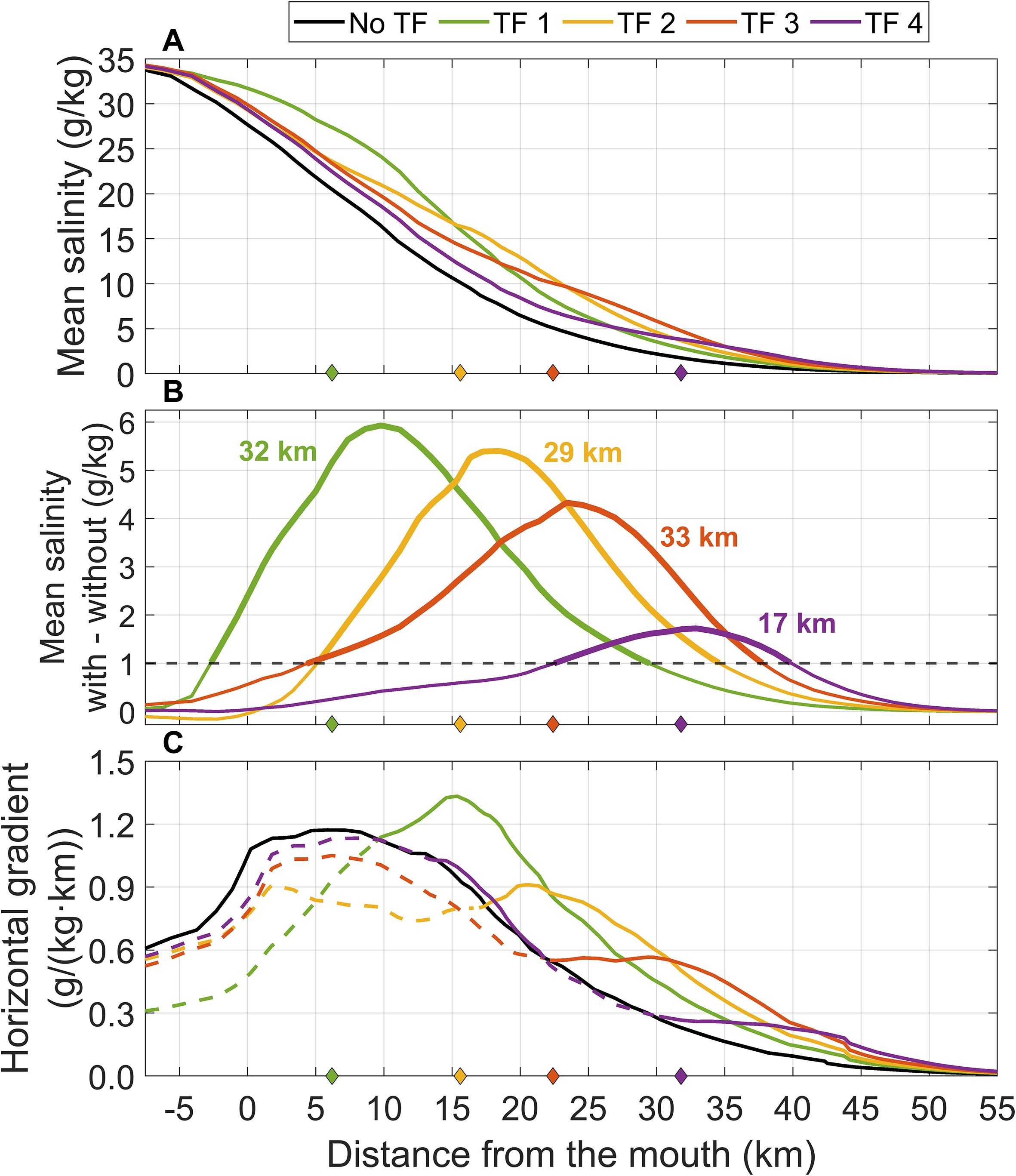
Figure 11. (A) Along-channel time-averaged salinity for the reference case (no tidal flat) and the four tidal flats (TF1, TF2, TF3, and TF4). (B) Along-channel time-averaged salinity differences (with minus without tidal flat). Regions of tidal flat influence, defined as the region where the salinity difference is greater than ΔS₀ = 1 g/kg, are highlighted in bold, and the colored numbers indicate their extent. (C) Along-channel horizontal salinity gradient for the reference case and the four cases analyzed. Dashed and solid lines highlight the portions of the estuary where the gradient with tidal flats is smaller and larger, respectively, compared to the gradient without them. The locations of the tidal flats are indicated by the colored diamonds.

7 Recapitulation and conclusions

This study examines the influence of hypothetical tidal flats with simplified geometries on the tidal and salinity dynamics of an estuary system, the Guadalquivir estuary. To achieve this, different parameters are configured, based on their location, extent, connection with the estuary and depth. The impact of each degree of freedom on the dynamics of the estuary and the salt plug is assessed through the analysis of key variables such as water level, salinity, and volume transport. In general, and for the selected configurations (which encompass a vast range of possibilities), a 10% change —used here as a convenient, though ultimately arbitrary, quantitative reference rather than an ecological or operational threshold—serves as an indicative upper limit for the alterations observed in these variables. The location and bathymetry of the tidal flats emerge as the most influential factors in this regard. This result aligns with the findings of Fortunato et al. (1999) for the mesotidal Tagus estuary, where energy dissipation in the tidal flats was found to be relatively insignificant, amounting to approximately 5% of the energy input into the system. The resulting variations in the tidal and saline dynamics are therefore minor compared to other factors, such as high discharges in Alcalá del Río dam (Díez-Minguito et al., 2013).

Overall, the implementation of a tidal flat in the estuary significantly alters its hydrodynamic regime. On one hand, the tidal flat increases water transport through the estuary mouth by expanding the effective surface area, thereby enhancing the tidal prism. On the other hand, its presence leads to increased friction, which reduces tidal amplitude and delays tidal wave propagation. This delay manifests as an increased phase shift between upstream and downstream sections, resulting in longer transit times throughout the estuary. These tidal patterns are consistent with those produced by increased friction in the estuary (Muñoz-López et al., 2024), demonstrating that the implementation of a tidal flat is dynamically equivalent to increasing friction within the estuary. From the perspective of numerical model calibration, this finding is highly significant, as omitting features such as obsolete channels, flood zones, or minor branches from the numerical domain could alter the model’s predicted results.

The sensitivity of these effects to tidal flat morphology is clearly demonstrated. Deeper tidal flats and larger inlets produce more pronounced modifications in both water transport and tidal wave characteristics, whereas the overall area of the tidal flat plays a relatively minor role. For example, the M₂ amplitude can increase by up to 9.5% under extreme configurations (i.e., largest area and inlet, and deepest bathymetry), and the phase delay can reach approximately 18 minutes in the most upstream location. The bathymetry of the tidal flat significantly influences the water exchange between the tidal flat and the estuary, as it establishes the drainage limit. Deeper bathymetries (e.g., -1 m) cause more diffuse effects, while shallower bathymetries (e.g., -0.5 m, 0 m) lead to delayed drainage and asymptotic-like behavior in the water level curves. Tidal flats with a bathymetry of +0.5 m, which are only flooded when the estuary water level exceeds this elevation, do not produce significant changes.

Moreover, the tidal flat’s location further modulates its impact. Tidal flats closer to the estuary mouth cause a more marked decrease in mean water level downstream of the inlet and larger increases in volume transport through the estuary mouth, while tidal flats located farther upstream exhibit greater reductions in tidal amplitude (up to 10 cm in the most upstream case) and longer transit times. As the tidal flat is located farther upstream, the increase in water transport diminishes, not due to reduced water uptake, but because the tidal amplitude itself decreases as the tidal flat moves further inland. Similarly, the phase difference between upstream and downstream sections is also greater when the tidal flat is near the mouth, supporting its role as an additional frictional source.

Salinity is affected by these hydrodynamic changes. The presence of a tidal flat in the estuary increases the mean salinity compared to a reference case without it, with the most significant increase observed approximately 3–4 km upstream of the tidal flat inlet. The peak salinity increase occurs just upstream of the inlet, establishing a region of tidal flat influence—defined in this study as the portion of the estuary where the mean salinity with the tidal flat exceeds the reference value by 1 g/kg. In this region, the tidal flat homogenizes the salinity field by reducing the salinity gradient downstream and increases it upstream of the tidal flat, which leads to a notable decrease in salinity fluctuations downstream and an increase upstream. Tidal flat morphology also plays a critical role. The depth of the tidal flat has a more significant effect on salinity than its overall area, with deeper tidal flats producing higher mean-salinity peaks. Moreover, the region of tidal flat influence extends further upstream for deeper tidal flats and larger inlets. When tidal flats are located closer to the estuary mouth, the region of influence can reach ~30 km; conversely, as the tidal flat is located farther inland, the downstream reduction and upstream intensification of the salinity gradient become less pronounced, resulting in smaller changes in tidal salinity amplitudes.

It is important to note that the developed model can be used to derive general conclusions about tidal propagation and salinity distribution in response to different tidal flat scenarios. Nonetheless, the model has inherent limitations. One such limitation is the simplification of the tidal flat geometry. Idealizing it on a regular grid may generate anomalous behavior in tidal dynamics, and the configuration of the estuarine connection does not fully reflect the complexity of a natural system. Further studies exploring different types and numbers of connections are needed. Another limitation is that the analysis does not consider any tidal–fluvial interaction effects, as freshwater discharges were set to constant values. The analysis focused solely on low river flow conditions, during which tidal-fluvial interactions are negligible in most of the estuary. Moreover, the current model does not account for sediment transport or vegetation dynamics, which are known to play significant roles in tidal flat evolution and hydrodynamics. Incorporating these factors in future studies would improve understanding of tidal flat restoration and resilience under changing environmental conditions. Despite these limitations, the model remains a valuable tool for assessing the potential impacts of tidal flat modifications on estuarine dynamics, particularly in regions with similar hydrodynamic conditions.

The present model provides a robust foundation for further investigations, such as incorporating additional physical variables (e.g., temperature) or integrating more realistic tidal flat restoration and management scenarios within the Guadalquivir estuary. It also serves as a basis for biological, ecological, geological, and even socio-cultural studies. The results highlight that estuarine hydrodynamics and salinity patterns are particularly sensitive to the tidal flat’s location and bathymetry, suggesting that restoration efforts and sustainable management policies should carefully consider site and depth selection. From a management perspective, these findings could inform decisions relating to estuarine habitat restoration, navigation, and water quality control, ultimately contributing to more effective and sustainable coastal planning.

Data availability statement

The raw data supporting the conclusions of this article will be made available by the authors, without undue reservation.

Author contributions

PM-L: Conceptualization, Methodology, Writing – review & editing, Investigation, Software, Writing – original draft, Formal Analysis, Visualization, Data curation, Validation. JG-L: Supervision, Writing – original draft, Funding acquisition, Writing – review & editing, Project administration, Formal Analysis, Conceptualization. IN: Writing – review & editing, Visualization, Software, Formal Analysis. SS: Visualization, Formal Analysis, Writing – review & editing, Software.

Funding

The author(s) declare that financial support was received for the research and/or publication of this article. Financial support from the Port Authority of Seville project 2020-ES-TM-0038-S (Optimization of the accessibility conditions) through the Connecting Europe Announcement (2020) is acknowledged. PM-L acknowledges the contract ascribed to this project.

Acknowledgments

Model runs have been carried out in the Supercomputing and Bioinnovation Center of the University of Malaga (PICASSO). We thank Puertos del Estado and Confederación Hidrográfica del Guadalquivir for making freely available the water-level and salinity data used to validate and calibrate the numerical model.

Conflict of interest

The authors declare that the research was conducted in the absence of any commercial or financial relationships that could be construed as a potential conflict of interest.

Generative AI statement

The author(s) declare that Generative AI was used in the creation of this manuscript. DeepL Write and ChatGPT have been used for improving the grammar and orthography.

Publisher’s note

All claims expressed in this article are solely those of the authors and do not necessarily represent those of their affiliated organizations, or those of the publisher, the editors and the reviewers. Any product that may be evaluated in this article, or claim that may be made by its manufacturer, is not guaranteed or endorsed by the publisher.

Supplementary material

The Supplementary Material for this article can be found online at: https://www.frontiersin.org/articles/10.3389/fmars.2025.1608858/full#supplementary-material

Abbreviations

GE, Guadalquivir estuary; SAIH, Automatic database of hydrological information for river flood management; TFn, Tidal Flat, with n from 1 to 4; SM Section of the Mouth; DS, Downstream Section; US, Upstream Section.

References

Álvarez O., Tejedor B., and Vidal J. (2001). La dinámica de marea en el estuario del Guadalquivir: un caso peculiar de «resonancia antrópica. Física Tierra 13, 11–24.

Google Scholar

Bermúdez M., Vilas C., Quintana R., González-Fernández D., Cózar A., and Díez-Minguito M. (2021). Unravelling spatio-temporal patterns of suspended microplastic concentration in the Natura 2000 Guadalquivir estuary (SW Spain): Observations and model simulations. Mar. pollut. Bull. 170, 112622. doi: 10.1016/j.marpolbul.2021.112622

PubMed Abstract | Crossref Full Text | Google Scholar

Billah M., Bhuiyan M. K. A., Islam M., Das J., and Hoque A. T. M. (2022). Salt marsh restoration: an overview of techniques and success indicators. Environ. Sci. pollut. Res. 29, 15347–15363. doi: 10.1007/s11356-021-18305-5

PubMed Abstract | Crossref Full Text | Google Scholar

Calvo J., Martín D., Morales-Martín G., and Viana S. (2018). HARMONIE-AROME, modelo operativo de escala convectiva de AEMET. Parte I: Modelo de predicción y validación. Acta las Jornadas Científicas la Asociación Meteorológica Española 1. doi: 10.30859/ameJrCn35p117

Crossref Full Text | Google Scholar

Chen Z. L. and Lee S. Y. (2022). Tidal flats as a significant carbon reservoir in global coastal ecosystems. Front. Mar. Sci. 9. doi: 10.3389/fmars.2022.900896

Crossref Full Text | Google Scholar

Couto I., Picado A., Des M., López-Ruiz A., Díez-Minguito M., Díaz-Delgado R., et al. (2024). Climate change and tidal hydrodynamics of guadalquivir estuary and doñana marshes: A comprehensive review. J. Mar. Sci. Eng. 12, 1443. doi: 10.3390/jmse12081443

Crossref Full Text | Google Scholar

Deltares (2022). “Delft3D-FLOW: Simulation of multi-dimensional hydrodynamic flows and transport phenomena, including sediments,” in User Manual. Hydro-Morphodynamics. Version: 3.15 SVN revision (Deltares, Boussinesqweg, The Netherlands).

Google Scholar

Díez-Minguito M., Baquerizo A., Ortega-Sánchez M., Navarro G., and Losada M.Á (2012). Tide transformation in the Guadalquivir estuary (SW Spain) and process-based zonation. J. Geophysical Res. 117, C03019. doi: 10.1029/2011JC007344

Crossref Full Text | Google Scholar

Díez-Minguito M., Contreras E., Polo M. J., and Losada M. A. (2013). Spatio-temporal distribution, along-channel transport, and post-river flood recovery of salinity in the Guadalquivir estuary (SW Spain). J. Geophysical Research: Oceans 118, 2267–2278. doi: 10.1002/jgrc.20172

Crossref Full Text | Google Scholar

Donázar-Aramendía I., Sánchez-Moyano J. E., García-Asencio I., Miró J. M., Megina C., and García-Gómez J. C. (2018). Maintenance dredging impacts on a highly stressed estuary (Guadalquivir estuary): a BACI approach through oligohaline and polyhaline habitats. Mar. Environ. Res. 140, 455–467. doi: 10.1016/j.marenvres.2018.06.009

PubMed Abstract | Crossref Full Text | Google Scholar

Fortunato A. B., Oliveira A., and Baptista A. M. (1999). On the effect of tidal flats on the hydrodynamics of the Tagus estuary. Oceanologica Acta 22, 31–44. doi: 10.1016/S0399-1784(99)80030-9

Crossref Full Text | Google Scholar

Gallego-Fernández J. and Novo F. (2006). High-intensity versus low-intensity restoration alternatives of a tidal marsh in Guadalquivir Estuary, SW Spain. Ecol. Eng. 30, 112–121. doi: 10.1016/j.ecoleng.2006.11.005

Crossref Full Text | Google Scholar

Geyer W. R. and MacCready P. (2014). The estuarine circulation. Annu. Rev. Fluid Dynamics 46, 175–197. doi: 10.1146/annurev-fluid-010313-141302

Crossref Full Text | Google Scholar

ITI Cádiz (2023). Puesta en valor del turismo ornitológico. Restoration of saltwork structures in Bahía de Cádiz Natural Park. Integrated Territorial Investment for Cádiz Province, (2014–2020 Partnership Agreement). Available online at: https://iticadiz.es/proyecto/puesta-en-valor-del-turismo-ornitologico/ (Accessed January 15, 2025).

Google Scholar

Li H., Li L., Su F., Wang T., and Gao P. (2021). Ecological stability evaluation of tidal flat in coastal estuary: A case study of Liaohe estuary wetland, China. Ecol. Indic. 130, 108032. doi: 10.1016/j.ecolind.2021.108032

Crossref Full Text | Google Scholar

Mahavadi T., Seiffert R., Kelln J., and Fröhle P. (2024). Effects of sea level rise and tidal flat growth on tidal dynamics and geometry of the Elbe estuary. Ocean Sci. 20, 369–388. doi: 10.5194/os-20-369-2024

Crossref Full Text | Google Scholar

Moral Ituarte L. D. (1993). El cultivo de arroz en las marismas de Doñana situación actual y perspectivas. Agricultura y Sociedad 67, 205–233.

Google Scholar

Muñoz-López P., Nadal I., García-Lafuente J., Sammartino S., and Bejarano A. (2024). Numerical modeling of tidal propagation and frequency responses in the Guadalquivir estuary (SW, Iberian Peninsula). Continental Shelf Res. 279, 105275. doi: 10.1016/j.csr.2024.105275

Crossref Full Text | Google Scholar

Murray N. J., Phinn S. R., DeWitt M., Ferrari R., Johnston R., Lyons M. B., et al. (2019). The global distribution and trajectory of tidal flats. Nature 565, 222–225. doi: 10.1038/s41586-018-0805-8

PubMed Abstract | Crossref Full Text | Google Scholar

Romero-Jiménez E., García-Valdecasas Ojeda M., Rosa-Cánovas J. J., Yeste P., Castro-Díez Y., Esteban-Parra M. J., et al. (2022). Hydrological response to meteorological droughts in the guadalquivir river basin, Southern Iberian Peninsula. Water 14, 2849. doi: 10.3390/w14182849

Crossref Full Text | Google Scholar

Ruiz J., Macías D., Losada M. A., Díez-Minguito M., and Prieto L. (2013). A simple biogeochemical model for estuaries with high sediment loads: Application to the Guadalquivir River (SW Iberia). Ecol. Model. 265, 194–206. doi: 10.1016/j.ecolmodel.2013.06.019

Crossref Full Text | Google Scholar

Ruiz J., Macías D., and Navarro G. (2017). Natural forcings on a transformed territory overshoot thresholds of primary productivity in the Guadalquivir estuary. Continental Shelf Res. 148, 199–207. doi: 10.1016/j.csr.2017.09.002

Crossref Full Text | Google Scholar

Siles-Ajamil R., Díez-Minguito M., and Losada M. (2019). Tide propagation and salinity distribution response to changes in water depth and channel network in the Guadalquivir River Estuary: an exploratory model approach. Ocean Coast. Manage. 174, 92–107. doi: 10.1016/j.ocecoaman.2019.03.015

Crossref Full Text | Google Scholar

van der Werf J., Reinders J., van Rooijen A., Holzhauer H., and Ysebaert T. (2015). Evaluation of a tidal flat sediment nourishment as estuarine management measure. Ocean Coast. Manage. 114, 63–74. doi: 10.1016/j.ocecoaman.2015.06.006

Crossref Full Text | Google Scholar

Yeste P., Dorador J., Martin-Rosales W., Molero E., Esteban-Parra M. J., and Rueda F. J. (2018). Climate-driven trends in the streamflow records of a reference hydrologic network in Southern Spain. J. Hydrology 566, 55–72. doi: 10.1016/j.jhydrol.2018.08.063

Crossref Full Text | Google Scholar