Abstract
Ongoing climate change is expected to transform ecosystems worldwide. Time series of remotely sensed data are now of sufficient length to begin to assess change in the ocean at large spatial and temporal scales. This study focused on changes in the phytoplankton phenology and composition in the subarctic Pacific Ocean, winter residence region for Pacific salmonids. A time series of satellite phytoplankton phenology metrics and phytoplankton functional groups between 2002 and 2022 were analyzed. Additionally, potential drivers of change were determined among the essential environmental factors and climate indices. Using changepoint analysis, a decrease in the total bloom length was revealed in recent years in all bioregions except for the waters surrounding the Kamchatka Peninsula. Moreover, a decreasing trend in the diatom-to-dinoflagellate Chl-a and the diatom-to-small algae Chl-a, consisting of haptophytes, pelagophytes, green algae, and cyanobacteria, was observed in the Gulf of Alaska. A sharp decline was particularly pronounced after 2018, which probably stemmed from a combination of the weaker currents forming the North Pacific Gyre Oscillation (NPGO) and recurring marine heat waves after 2014. It is uncertain yet whether the decline of the diatom group is temporary or marks the beginning of a long-term shift in the phytoplankton community structure in the subarctic Pacific. The following years will likely bring the answers.
1 Introduction
A significant reduction of marine biodiversity is predicted in the coming years due to climate change, which may affect ecosystem stability and lead to their profound reorganization and possible loss of some ecosystem services (Irwin et al., 2015; Henson et al., 2021). Thus far, global observations indicate a significant decline in phytoplankton biomass over the last century, at an estimated decrease of approximately 1% of the worldwide median per year. However, this trend is not uniform across regions (Boyce et al., 2010). Regional differences may arise from spatial variations in environmental change (Doney et al., 2012; Thomas et al., 2012), and thus variable response of phytoplankton biomass and community composition at regional scales (Wyatt et al., 2022). Plankton communities consist of complex aggregations of organisms that interact in various ways, including competition for scarce resources and grazing on one another (Laufkötter et al., 2013; Cael et al., 2021; Taves et al., 2022). As phytoplankton respond rapidly to fluctuations in light field and water properties (Winder and Sommer, 2012; Litchman et al., 2012), ecological changes can happen abruptly rather than gradually, making it crucial to identify early warning signs (Scheffer et al., 2009; Cael et al., 2021) and develop conservation plans before the ecosystems reach a tipping point.
Identifying changes and early warning signals requires comprehensive long-term monitoring and practical information synthesis and communication (Williams et al., 2020). To meet these needs, new large-scale phytoplankton monitoring approaches have been developed, often utilizing satellite data, which is well-suited for broad seasonal and interannual observations (Losa et al., 2017; Moisan et al., 2017). Monitoring seasonal and interannual shifts in the ecosystems is often based on biogeography, which focuses on spatially distinct regional aggregations governed by mixed effects of physical and biological interactions shaping fauna and flora, frequently referred to as bioregions (Lourie and Vincent, 2004; UNESCO, 2009; Kavanaugh et al., 2014). Within bioregions, the diverse seascape may be described by conservative (temperature or salinity) and non-conservative (nutrient concentrations) water properties (Oliver and Irwin, 2008), better highlighting characteristics of the drivers of phytoplankton abundance and community composition (Konik et al., 2024).
A major factor controlling primary productivity and shaping phytoplankton communities in the subarctic Pacific is iron (Fe) concentration since it is one of the High Nutrient, Low Chlorophyll (HNLC) regions of the World Ocean (Nishioka et al., 2020). While the subarctic North Pacific Ocean is generally dominated by haptophytes and green algae, the western sector receives macronutrients and iron from the Okhotsk Sea and the Oyashio current that support intense spring diatom blooms, especially south of Hokkaido (Obayashi et al., 2001). Following the spring bloom, nutrient depletion leads to a higher contribution of picoeukaryotes and Synechococcus in late summer (Harrison et al., 2004; Liu et al., 2004). In the Eastern Pacific Ocean, iron concentrations are lower, with little seasonal variation (Peña and Varela, 2007), and haptophytes and pelagophytes are the primary contributors to phytoplankton biomass, while diatoms are secondary contributors (Harrison, 2002; Harrison et al., 2004; Peña et al., 2019) since they are sensitive to iron limitation (Sarthou et al., 2005).
Decadal variability in phytoplankton biomass in the subarctic Pacific has been linked to climate indices, including the Pacific Decadal Oscillation (PDO) (Martinez et al., 2009) and the North Pacific Gyre Oscillation (NPGO) (Xiu and Chai, 2012). Additionally, the seasonal variability in phytoplankton abundance — referred to as phytoplankton phenology (Isles and Pomati, 2021) — has also been shown to be affected by these climate oscillations (Suchy et al., 2019). Significant role in shaping phytoplankton phenology patterns play large groups, primarily diatoms and dinoflagellates (Falkowski et al., 2004), which are major contributors to the flux of organic matter up the trophic levels. Therefore, changes in diatom biomass and bloom time can have cascading effects on higher trophic levels, when a match/mismatch between the peaks of phytoplankton and zooplankton biomass happens (Hjort, 1926; Cushing, 1990; Malick et al., 2015; Suchy et al., 2022). Relationships among the PDO, NPGO, phytoplankton abundance, and Pacific salmon productivity have been noted by Mantua et al. (1997) and Litzow et al. (2018). Moreover, the balance among phytoplankton groups can be significantly disrupted by extreme events such as marine heat waves, which have been observed to decrease the ratio of large to small phytoplankton (Wyatt et al., 2022). The frequency and intensity of the extreme events are predicted to increase with climate change (Frölicher and Laufkötter, 2018), and there is, therefore, an urgent need to understand how these and other climate changes are impacting the subarctic Pacific Ocean, and the regional variability of these impacts.
The goal of this study was to identify the change and the potential factors driving variability in chlorophyll-a (Chl-a) concentration, which serves as a proxy for phytoplankton abundance (Huot et al., 2007), as well as for phytoplankton phenology and composition in the subarctic Pacific. To achieve this goal, the analysis was conducted at the bioregional scale in the subarctic Pacific, following the classification by Konik et al. (2024). This approach enabled the identification of the main physical drivers specific to each bioregion, which will help assess pressures on local populations more accurately. A region-specific framework like this is crucial for strengthening resilience and managing diverse marine habitats (Lourie and Vincent, 2004; Marchese et al., 2022). Considering the importance of the diatoms in the global biological carbon pump and the intense zooplankton grazing in the subarctic Pacific (Liu et al., 2016), particular emphasis was put on the diatom group in this research. Diatoms also significantly contribute to the spring blooms in the North Pacific (Clemons and Miller, 1984; Fiechter et al., 2009; Peña et al., 2019; Taves et al., 2022) and introduce large Chl-a loads, especially on the North Pacific shelf (Peterson and Harrison, 2012). A specific term has been coined for the diatom contribution— the “extra diatom input” (Obayashi et al., 2001) — contrasting with the “basic” phytoplankton composition consisting of the small-celled haptophytes, pelagophytes, and green algae, showing stable abundance throughout the year and across the subarctic Pacific Ocean compared to diatoms (Suzuki et al., 2002; Alvain et al., 2005).
To put in the context changes in the diatom contribution, we presented the anomaly of the proportion between diatoms and dinoflagellates, and between diatoms and small algae, defined as haptophytes, pelagophytes, green algae, and cyanobacteria. This approach was adopted not only based on the cell size differences but also to highlight implications for the ecosystem due to differences in the nutrient source. Small algae are more reliant on recycled nutrients, contributing more to regenerated production rather than the new production (Price et al., 1994; Meyer et al., 2022).
2 Data and methods
2.1 Study area
In the subarctic North Pacific Ocean, circulation in the upper part of the water column is dominated by two major gyres, the Alaskan Gyre (AG) in the east and the Western Subarctic Gyre (WSG) in the west, outlining the subarctic Pacific (Fukuwaka et al., 2004). A combination of the geostrophic transport, Ekman pumping and vertical mixing within the gyres provides regular winter nutrient enrichment to the upper layer (Capotondi et al., 2005; Nakanowatari et al., 2017). As a result, the subarctic Pacific is one of the three HNLC zones (Harrison et al., 1999; Liu et al., 2004), where phytoplankton dynamics is generally controlled by grazing (Strom and Welschmeyer, 1991) and Fe supply into the epipelagic waters (Sarmiento et al., 2004). Most of the external iron is transported with the subsurface waters from the shelf, shallow enough to be brought up to the surface by winter upwelling and vertical mixing (Lam and Bishop, 2008). Shelf areas also receive Fe with sediment resuspension and land runoff, fuelled mainly by snowmelt in spring and glacier meltwater in summer (Davis et al., 2014; Crusius et al., 2017), primarily where the drainage basins are composed of Fe-bearing volcanic rocks like in the Kuril/Kamchatka region (Lam and Bishop, 2008). The macronutrient and Fe-rich waters critical for primary production (PP) are transported offshore by the mesoscale eddies formed regularly in the Gulf of Alaska (GoA) (Whitney et al., 2005), around the Kamchatka Peninsula (Rogachev et al., 2007), and in the convergence zone of the Kuroshio and Oyashio currents on the Japanese coast (Ueno et al., 2023). Another major source of Fe in the subarctic Pacific is atmospheric deposition, consisting of the Fe-rich dust transported regularly from the Asian deserts (Duce and Tindale, 1991), occasionally emitted volcanic ashes (Hamme et al., 2010), and relatively recently acknowledged Alaskan glacial dust (Crusius, 2021) and excess dust of anthropogenic origin (Pinedo-González et al., 2020; Hunt et al., 2024).
The above processes, coupled with seasonal light availability, shape phytoplankton biomass and phenology in the subarctic Pacific, and remain in a delicate balance susceptible to climate oscillations (Mueter et al., 2004). A key driver of ocean conditions in the subarctic Pacific is the Aleutian Low, a vast low-pressure atmospheric system that dominates the region in winter, controlling the strength of the westerly winds and impacting the winter convective mixing and nutrient replenishment in the euphotic zone (Goes et al., 2004). The strength of subsequent ocean forcing of the Aleutian Low is strongly related to climate indices, including the El Niño–Southern Oscillation (ENSO) (Ortiz-Tánchez et al., 2002; Zhang et al., 2019), the Pacific Decadal Oscillation (PDO) (Bond and Harrison, 2000), and the North Pacific Gyre Oscillation (NPGO) (Di Lorenzo et al., 2008).
2.2 Satellite-derived phytoplankton phenology and composition
To describe phytoplankton variability, satellite-derived Chl-a concentrations were retrieved from the 25 km 8-day Globcolour product (ACRI-ST, 2017), based on level‐2 weighted averaging of surface chlorophyll-a (AVW) (O’Reilly et al., 2000; Pauthenet et al., 2024), composed of the SeaWiFS (1997 – 2010), MERIS (2002 – 2012), MODIS-Aqua (2002 – present), VIIRS-NPP (2012 – present), and VIIRS-JPSS-1 (2017 – 2022). The Globcolour-AVW dataset was used since it appeared to be the best-harmonized product out of the several existing merged products for climate studies (Pauthenet et al., 2024). Radiometric observations by Pauthenet et al. (2024) indicated that the Globcolour-GSM dataset had been significantly affected by the drift of the VIIRS sensor, while the OC-CCI dataset showed biases due to higher inputs from MODIS. Furthermore, the PFT validation performed against an independent flow cytometry dataset collected in 2022 confirmed good agreement between the PFT estimates and in situ data (Eisner and Lomas, 2022; Konik et al., 2024). The 25 km pixel size was sufficient for capturing spatial patterns in the subarctic Pacific, and the 8-day temporal resolution was considered optimum to increase cloud-free information required for the phytoplankton phenology analysis based on previous studies (Siswanto et al., 2022; Pramlall et al., 2023; Konik et al., 2024). Phytoplankton phenology metrics in the years 1998–2022 were determined following the methods described in detail by Konik et al. (2024). Generally, the pixels covered by clouds for more than 60% of the time were excluded, and at all the remaining locations, pixel-by-pixel, missing data was interpolated in time on a yearly basis to avoid extrapolation in January and December, the two most clouded months in the study area (Brody et al., 2013). The obtained time series were smoothed with a three-point median filter (Lavigne et al., 2018), and the phytoplankton blooms were identified using the median timelines extracted from a 3x3 pixel window (Konik et al., in prep). The Chl-a threshold method was used since it is preferred for the match/mismatch analysis between the trophic levels (Brody et al., 2013), where the baseline was established 5% above the climatology Chl-a median in the years 1998 – 2022, and bloom was detected only when Chl-a exceeded the baseline for at least two weeks (two consecutive maps) (Soppa et al., 2016; Suchy et al., 2022). Finally, the following phenology metrics were determined (Figure 1): (1) starting date of a bloom (Bstart), the day (Day of Year, DOY) when Chl-a exceeded the baseline for at least two consecutive measurements, with a particular emphasis on the first bloom of the year (FBstart); (2) end date of a bloom (Bend, DOY), which was the following date when Chl-a dropped below the baseline; (3) length of a bloom (BLen, the number of days), derived as the difference between the end and the beginning of a bloom; (4) the maximum Chl-a concentration during a bloom (Cmax, mg m–3), and (5) the time (Tmax, DOY) when maximum Chl-a concentration was observed (Soppa et al., 2016; Krug et al., 2018); (6) length of the bloom season (SLen, the number of days) was defined as the time elapsed between the start of the first bloom and the end of the last bloom; (7) the number of bloom days during each bloom was summed and given as the total bloom length (TotBLen, the number of days) (Krug et al., 2018); and (8) the Chl-a values during the bloom time were added together to estimate the bloom magnitude (Bmagn, mg m–3 year–1) (Soppa et al., 2016).
Figure 1
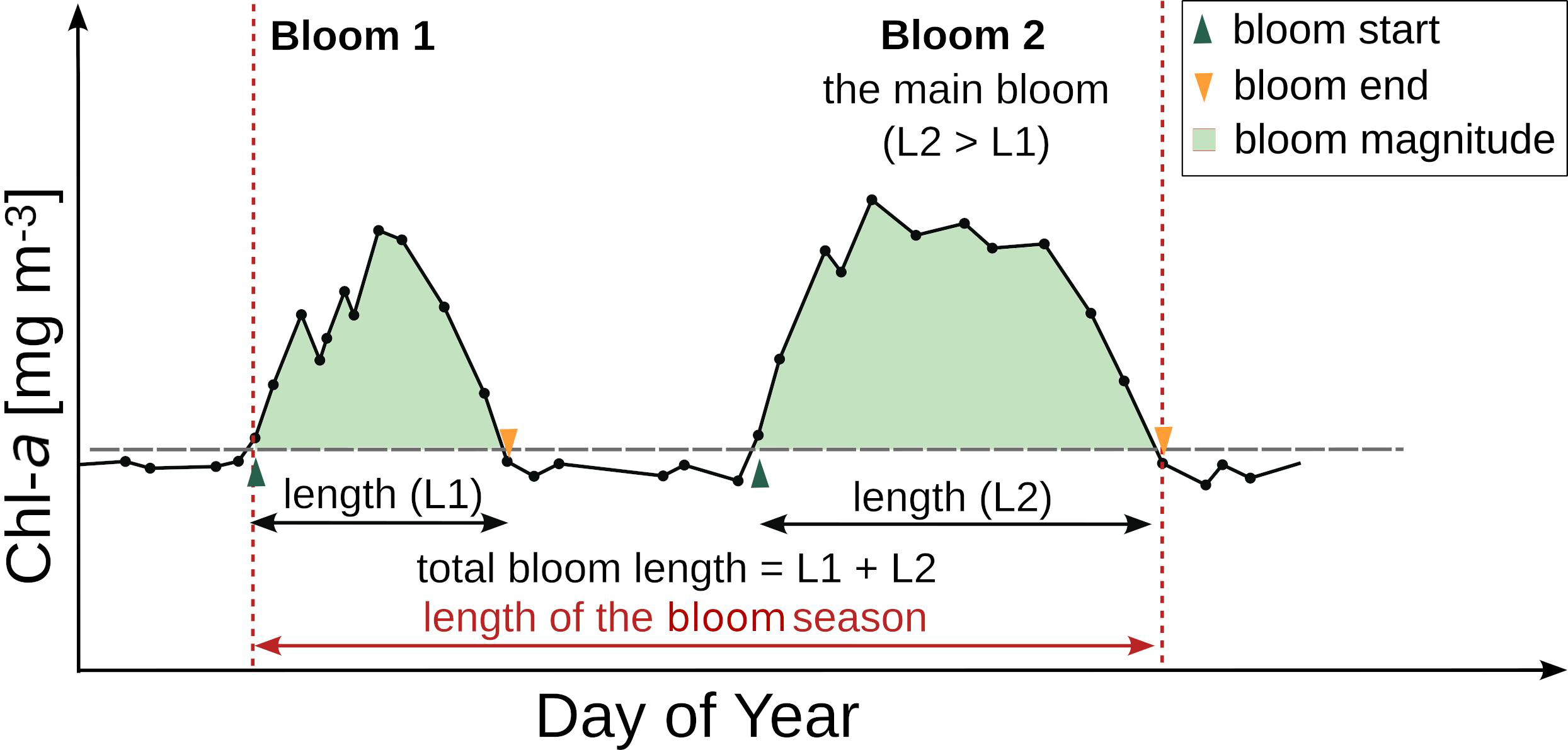
Schematic overview of the phenology metrics analyzed in this study (Konik et al., 2024). Source: adapted from Konik et al. (2024). Published under CC BY-NC-ND 4.0, Crown Copyright.
The phytoplankton composition, or phytoplankton functional types (PFT) (Bracher et al., 2017), from 2002 to 2022, was determined following the methods by Xi et al. (2020), as updated in Xi et al. (2021), but adapted for our regional application as in Konik et al. (2024). The retrieval of the satellite-based PFT time series involved three key steps. First, based on the pigment proportions and composition obtained using High-Performance Liquid Chromatography (HPLC), we determined the phytoplankton composition at the sampling stations with a chemotaxonomic model (CHEMTAX). Next, the identified groups were clustered into six main PFTs, which could be distinguished in the satellite images: diatoms, dinoflagellates, cryptophytes, cyanobacteria, green algae=chlorophytes and prasinophytes, and hapto+pelago=haptophytes and pelagophytes. Finally, an Empirical Orthogonal Function-based model was developed and validated with an independent dataset (Eisner and Lomas, 2022; Weitkamp et al., 2024), allowing for the computation of PFT maps for the entire study area. These satellite-derived PFTs were obtained using remote sensing reflectance (Rrs; sr–1) products from the GlobColour database across nine spectral bands centered at 412, 443, 469, 490, 531, 555, 645, 670, and 678 nm, and the Sea Surface Temperature (SST) daily maps at 0.25°x0.25° NOAA OISST v2 high-resolution data (Reynolds et al., 2002, 2007) provided by the NOAA/OAR/ESRL PSL, Boulder, Colorado, USA (NOAA, 2007). Among the six PFT, the main focus of this study was the ratio between the diatoms and the small-cell phytoplankton, composed of haptophytes, pelagophytes, green algae, and cyanobacteria. Additionally, the diatom to dinoflagellate Chl-a ratio was included since they are often presented as examples of the opposite survival adaptations to physical and nutritional forcing, captured by Margalef’s mandala (Gilbert and Burford, 2017).
2.3 Environmental drivers
The analysis considered two groups of environmental variables: (i) 2D-time series of the environmental parameters obtained from hydrodynamic models, including Sea Surface Temperature (SST), salinity, Sea Surface Height (SSH), Mixed Layer Depth (MLD), surface current speed (CurrS), and satellite-derived Photosynthetically Available Radiation (PAR); and (ii) time series of climate indices.
2.3.1 2D time series: hydrology
The SST (the NOAA OISST v2 high-resolution data set, Reynolds et al., 2002, 2007; Huang et al., 2021) was averaged seasonally (winter: January – March, spring: April – June, summer: July – September, and fall: October – December). The seasonal averages of the salinity, the SSH, the MLD, and the CurrS were determined based on the ARMOR3D reanalysis data (Guinehut et al., 2012; Mulet et al., 2012), downloaded from the Copernicus CMEMS portal (https://doi.org/10.48670/moi-00052). The PAR seasonal average and maximum were extracted from the MODIS AQUA L3 product (Frouin et al., 2012) published by the NASA Ocean Biology Processing Group (OBPG) (NASA, 2022).
2.3.2 1D time series: climate indices
The second group of data constituted a number of teleconnection indices, most commonly related in the literature to the variability of marine biotic and abiotic elements of the North Pacific, including: 1) the Southern Oscillation Index (SOI), which is the standardized difference in Sea Level Pressure (SLP) between Tahiti and Darwin, Australia (Trenberth, 1984); 2) the Multivariate El Niño–Southern Oscillation index (ENSO, MEIv2) (Zhang et al., 2019); 3) the Arctic Oscillation index (AO), defined as the first mode of the empirical orthogonal function (EOF) analysis of the monthly mean height anomalies at 1000-hPa (Thompson and Wallace, 1998; Ogi and Wallace, 2007); 4) the Pacific–North America (PNA) pattern, which describes the strength of the atmospheric pressure dipole between the Aleutian Low in the northern Pacific Ocean and the ridge over the western North America (Wallace and Gutzler, 1981); 5) the North Pacific Index, calculated as the area-weighted mean SLP over the region 30°N – 65°N, 160°E – 140°W (Trenberth and Hurrell, 1994); 6) the Pacific Decadal Oscillation (PDO), defined as the leading mode of the SST (Bond and Harrison, 2000); 7) the North Pacific Gyre Oscillation (NPGO), which is the second EOF mode of the North Pacific sea surface height anomalies (SSHa) (Di Lorenzo et al., 2008); and 8) the Aleutian Low‐Beaufort Sea Anticyclone (ALBSA), a four-point gradient calculated using the daily mean 850‐hPa geopotential heights (GPHs) (Cox et al., 2019). The SOI, MEIv2, AO, PNA, PDO, and ALBSA were obtained from the NOAA website (https://psl.noaa.gov/, last accessed: 2023-04-28), the NPI was downloaded from the NCAR Climate Data Guide website (https://climatedataguide.ucar.edu, last accessed: 2023-04-28), and the NPGO from the http://www.o3d.org/npgo/npgo.php website (last accessed: 2023-03-24).
2.4 Statistical analysis
The statistical significance of the long-term temporal trends in phytoplankton community structure in each bioregion was investigated using the non-parametric Mann-Kendall test (Hollander and Wolfe, 1973; Millard, 2013), and the abrupt changes in the phytoplankton phenology were determined using the changepoint method (Killick and Eckley, 2014; Killick et al., 2022), based on the pruned exact linear time (PELT) algorithm for the regime shift identification (Killick et al., 2012). The modified Bayesian information criterion (MBIC) was the penalty function of the changepoint analysis, guarding against small segments and allowing for any number of changes, including a ‘no change’ result.
To identify the key environmental factors driving phytoplankton phenology within bioregions, the multiple factor analysis (MFA) was performed using the factoextra R package (Kassambara and Mundt, 2020), which is based on the principal component analysis (PCA) (Le et al., 2008). Factors explaining 1% or less of the variability were excluded from the analysis and not presented in the results. The analyses were conducted with the numpy (Harris et al., 2020) and pandas (McKinney, 2010) Python libraries and R software (R Core Team, 2020) using the ggplot2 (Wickham, 2016), tidyverse (Wickham et al., 2019), gridExtra (Auguie and Antonov, 2017), RColorBrewer (Neuwirth and Maindonald, 2022), Kendall (McLeod, 2011), EnvStats (Millard, 2013), and Performance Analytics (Peterson et al., 2020) RCRAN packages.
2.5 Bioregions
All the analyses were performed at the scale of the bioregions, which were adapted from the original bioregions defined in Konik et al. (2024). For this, the original bioregions were subdivided into the eastern and western parts due to the impact of large-scale circulation patterns, namely the AG and the WSG, related to the spatial variability in the physical and chemical water properties in the subarctic Pacific (Harrison et al., 1999; Nishioka et al., 2021). Marginal and Connecting bioregions were split into the eastern and western parts as the previous study showed significant contrasts between the Eastern and Western Pacific with respect to hydrology, including the SST, and the zooplankton community structure (Chiba et al., 2015). For example, significant differences in the vertical stratification of the water column between the eastern and western North Pacific have been described in the literature (Old et al., 2019). Vertical stratification controls the mixed layer depth and, therefore, the nutrient concentrations in the upper ocean layer (Goes et al., 2004; Yasunaka et al., 2021); most importantly iron, which is the main nutrient limiting primary productivity within the HNLC zone in the subarctic Pacific (Zhang et al., 2021). The iron loads entering the WSG are significantly higher than those that supply the AG, mainly due to the water exchange with the adjacent seas, the Bering Sea and the Okhotsk Sea (Goes et al., 2004; Nishioka et al., 2020). Furthermore, the western subarctic Pacific is a highly dynamic region characterized by intense eddy activity and strong vertical mixing (Gaube et al., 2015; Siswanto et al., 2022). This is particularly evident in the Kuroshio-Oyashio Extension Region (KOER) near Japan (Itoh and Yasuda, 2010) and along the Kuril-Kamchatka Trench (Itoh and Yasuda, 2010), whereas the central part experiences relatively weaker vertical mixing (Gargett, 1991).
The resulting division consisted of the eight bioregions: Central South (CS), Central Oregon (CO), Central North (CN), Connecting East (ConE), Connecting West (ConW), Marginal East (MarE), Marginal West (MarW), and Archipelago (Arch) (Figure 2).
Figure 2
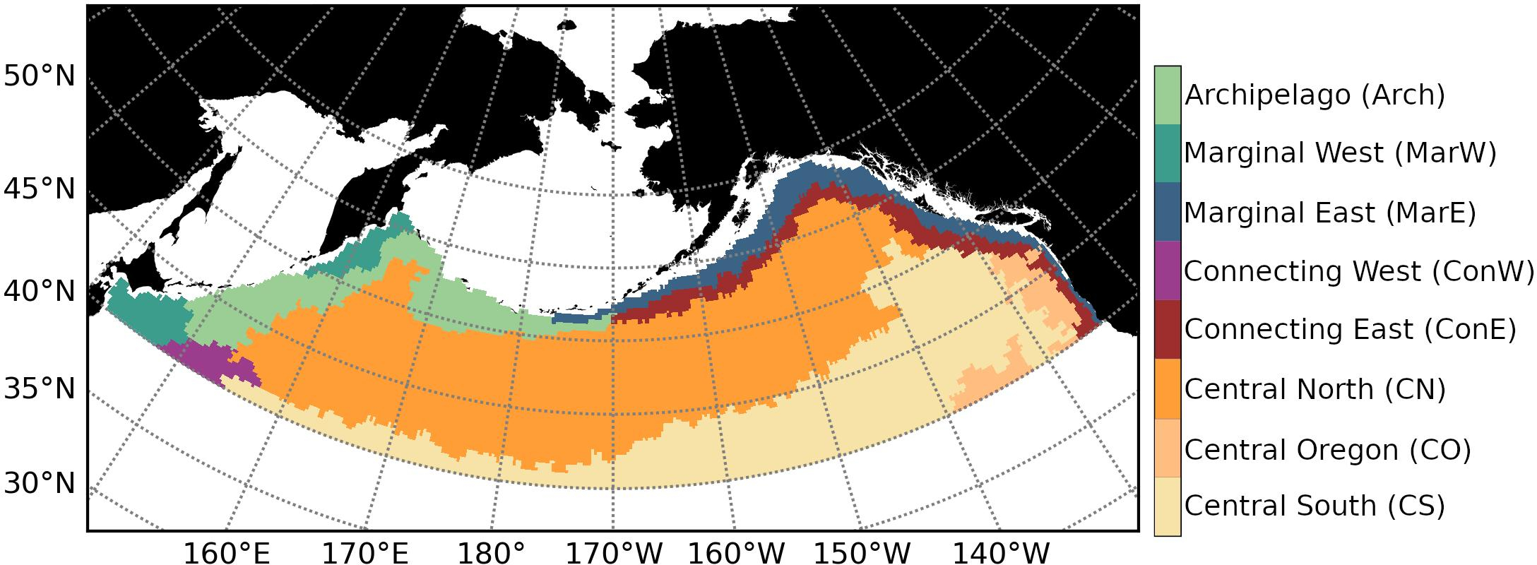
Bioregions. Source: adapted from Konik et al. (2024). Published under CC BY-NC-ND 4.0, Crown Copyright.
3 Results
3.1 Identifying changes in phytoplankton phenology
The interannual changes in the main phenology metrics, Bstart and Bend, from 1998 to 2022, generally did not show statistically significant long-term trends for the bioregions. However, a substantial change in the average total bloom length (TotBLen) was observed in recent years. The changepoint analysis revealed that the TotBLen decreased by between six weeks (bioregion CO) and two weeks (Arch) (Figures 3b, f). The largest decrease in the TotBLen, of 45 days, was observed in CO, where the Chl-a is generally low (<0.7 mg m–3). However, an evident drop in the TotBLen was also observed in the other bioregions where the Chl-a and related phytoplankton biomass is much higher (>1 mg m–3). For example, in the border of the Gulf of Alaska (ConE and MarE bioregions), the TotBLen was shorter by a month after 2014 (Figures 3d, h). The only bioregion where the TotBLen increased by almost two weeks was the MarW bioregion, bordering the Kamchatka Peninsula (Figure 3g), where changes were observed as early as 2001. This was followed by a decrease in TotBLen in the Arch bioregion in 2004 and the central bioregions between 2010 and 2013, with the latest change in the ConW in 2018 (Figure 3e).
Figure 3
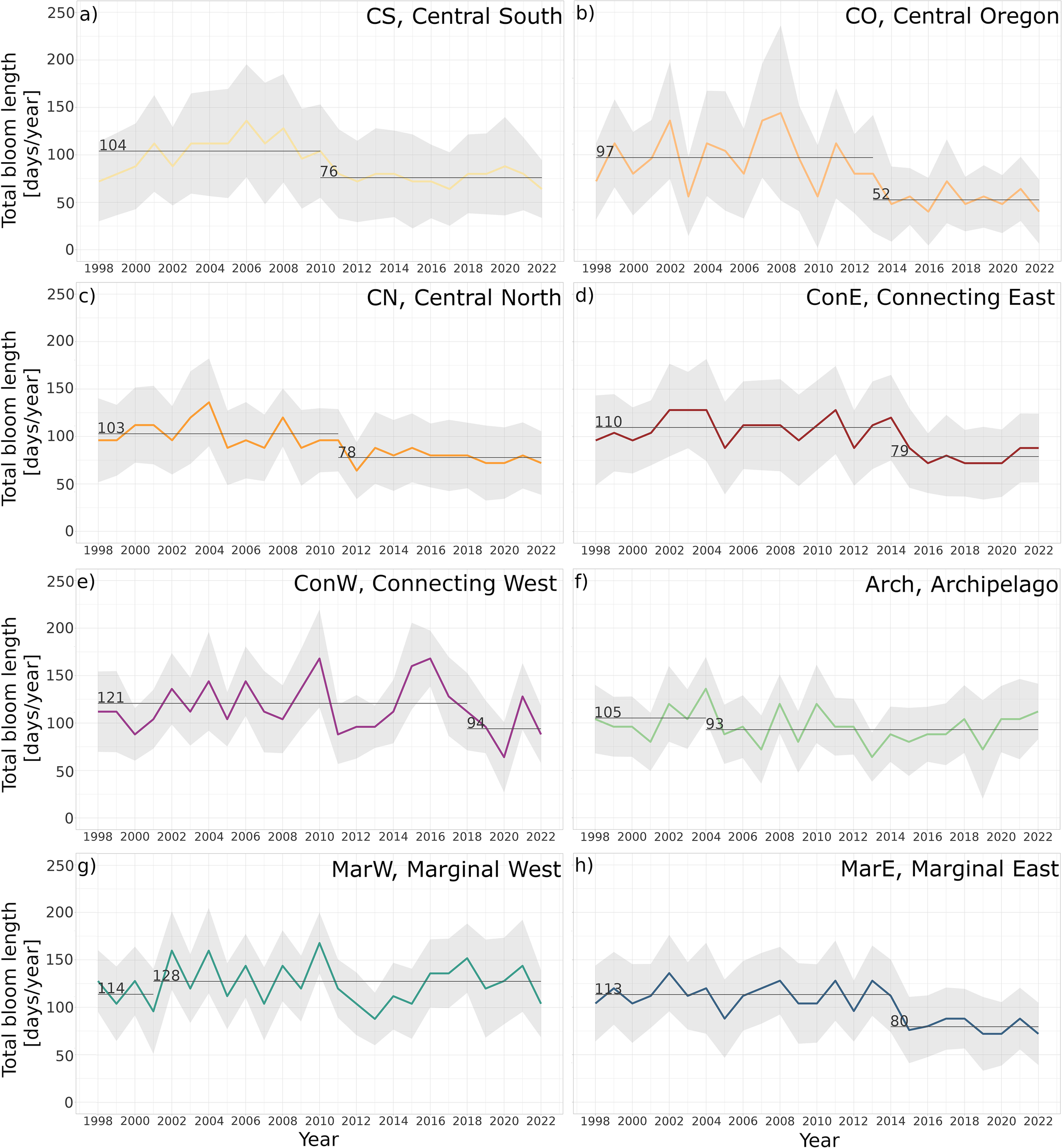
Total bloom length, TotBLen [days/year] in the years 1998–2022 within each region: (a) Central South, (b) Central Oregon, (c) Central North, (d) Connecting East, (e) Connecting West, (f) Archipelago, (g) Marginal West, (h) Marginal East. The horizontal lines indicate distinct regimes determined using the changepoint PELT method (Killick et al., 2012).
We found a relationship between the decrease in TotBLen and Chl-a. Using the Mann-Kendall test, we confirmed the statistical significance of the relationships between TotBLen and Cmax in bioregions CS, CO, ConE, MarE, and Arch (Figure 4). Thus, we may expect further decreases in TotBLen in the future should there be a change in total Chl-a levels, for example, resulting from a shift in phytoplankton composition.
Figure 4
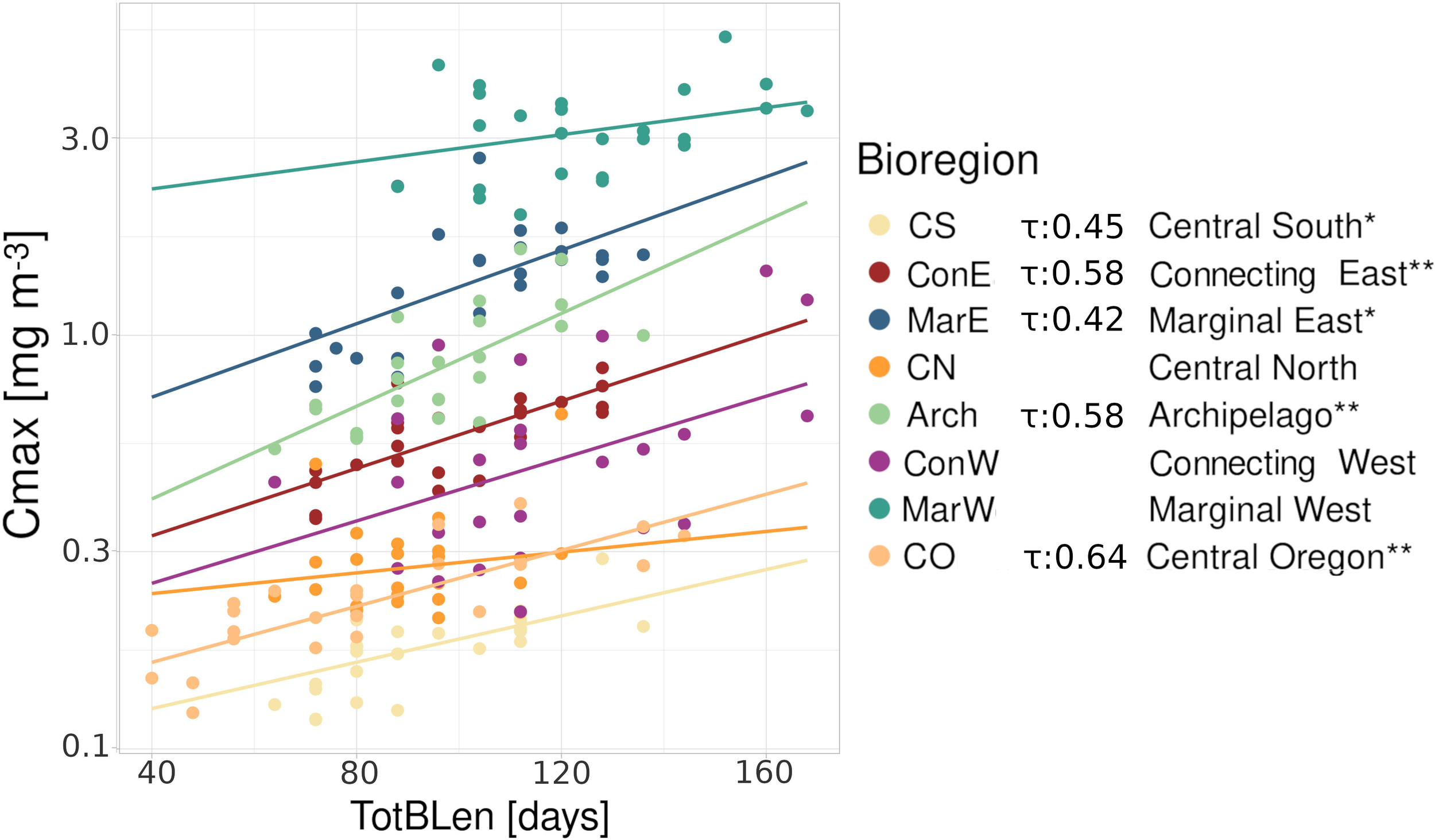
Relationship between Cmax [mg m–3] and TotBLen [days] from 1998 to 2022 within bioregions, with respective regression lines presented in matching colors. Bioregions where the relationships were statistically significant (the Mann-Kendall test: τ) are marked with stars (*p<0.01, **p<0.001).
3.2 Identifying changes in phytoplankton composition
A general decrease in diatom and cyanobacteria abundance in all bioregions and an increase in the hapto-pelago group, except for the CS bioregion, were statistically confirmed by the Mann-Kendall test with the seasonal correction (Table 1). No change in green algae was observed in the connecting bioregions ConE and ConW and marginal bioregions MarE, MarW, and Arch. Only a slight negative trend in dinoflagellates and cryptophytes was found in the ConE and MarE, bordering the Gulf of Alaska. As a result, negative trends in diatom-to-dinoflagellate and diatom-to-small algae Chl-a (haptophytes, pelagophytes, green algae, and cyanobacteria) were observed across the entire study area.
Table 1
| CS | CO | CN | ConE | ConW | MarE | MarW | Arch | |
|---|---|---|---|---|---|---|---|---|
| Diatoms | -0.51*** | -0.41*** | -0.49*** | -0.44*** | -0.28*** | -0.38*** | -0.25*** | -0.30*** |
| Dinoflagellates | -0.20*** | -0.21*** | -0.17*** | -0.16*** | -0.05 | -0.09* | 0.01 | 0.02 |
| Cryptophytes | -0.26*** | -022*** | -0.23*** | -0.17*** | -0.06 | -0.15** | -0.02 | -0.07 |
| Cyanophytes | -0.62*** | -0.58*** | -0.60*** | -0.62*** | -0.47*** | -0.55*** | -0.47*** | -0.46*** |
| Green algae | -0.29*** | -0.22*** | -0.11* | -0.11* | 0.04 | -0.04 | -0.01 | 0.08 |
| Hapto-pelago | -0.40*** | 0.36*** | 0.45*** | 0.43*** | 0.38*** | 0.44*** | 0.48*** | 0.49*** |
| Diato/Dino | -0.6*** | -0.52*** | -0.58*** | -0.55*** | -0.38*** | -0.47*** | -0.36*** | -0.43*** |
| Diato/Small Algae | -0.57*** | -0.52*** | -0.57*** | -0.56*** | -0.38*** | -0.50*** | -0.40*** | -0.45*** |
Trends in the Chl-a concentration (mg m–3) per phytoplankton group within each bioregion (2002 – 2022): Central South (CS), Central Oregon (CO), Central North (CN), Connecting East (ConE), Connecting West (ConW), Marignal East (MarE), Marginal West (MarW), and Archipelago (Arch), determined independently for each bioregion using the non-parametric Mann-Kendall test (with the correction for seasonal variability — kendallSeasonalTrendTest — RCRAN function) (Hirsch et al., 1982; McLeod, 2011), where *** is p<0.001, ** is p<0.01, * is p<0.05.
Each color corresponds to a specific bioregion, as introduced in Figure 2.
In the central bioregions, such as the CS, CO, and CN, the diatom-to-small-algae ratio anomaly was less pronounced than in the other bioregions due to relatively smaller input from diatoms (Figures 5a–c). However, between 2010 and 2013, negative anomalies were evident even in these bioregions (Figures 5a–c), which matches the timing of the regime shift in the TotBLen in the respective bioregions (Figure 3a–c). This match in time was also observed in the ConE and MarE bioregions (Figures 5d, h), where the negative anomalies co-occurred with the decrease in the TotBLen, around 2014 (Figures 3d, h), and in 2018 in the ConW bioregion (Figures 3e, 5e). The change in bioregions Arch and MarW was not as evident as in the others (Figures 5f, g). Still, the positive diatom-to-small-algae ratio anomaly peaks associated with diatom blooms were lower in the last decade, and periods with negative anomalies lasted longer, particularly after 2018.
Figure 5
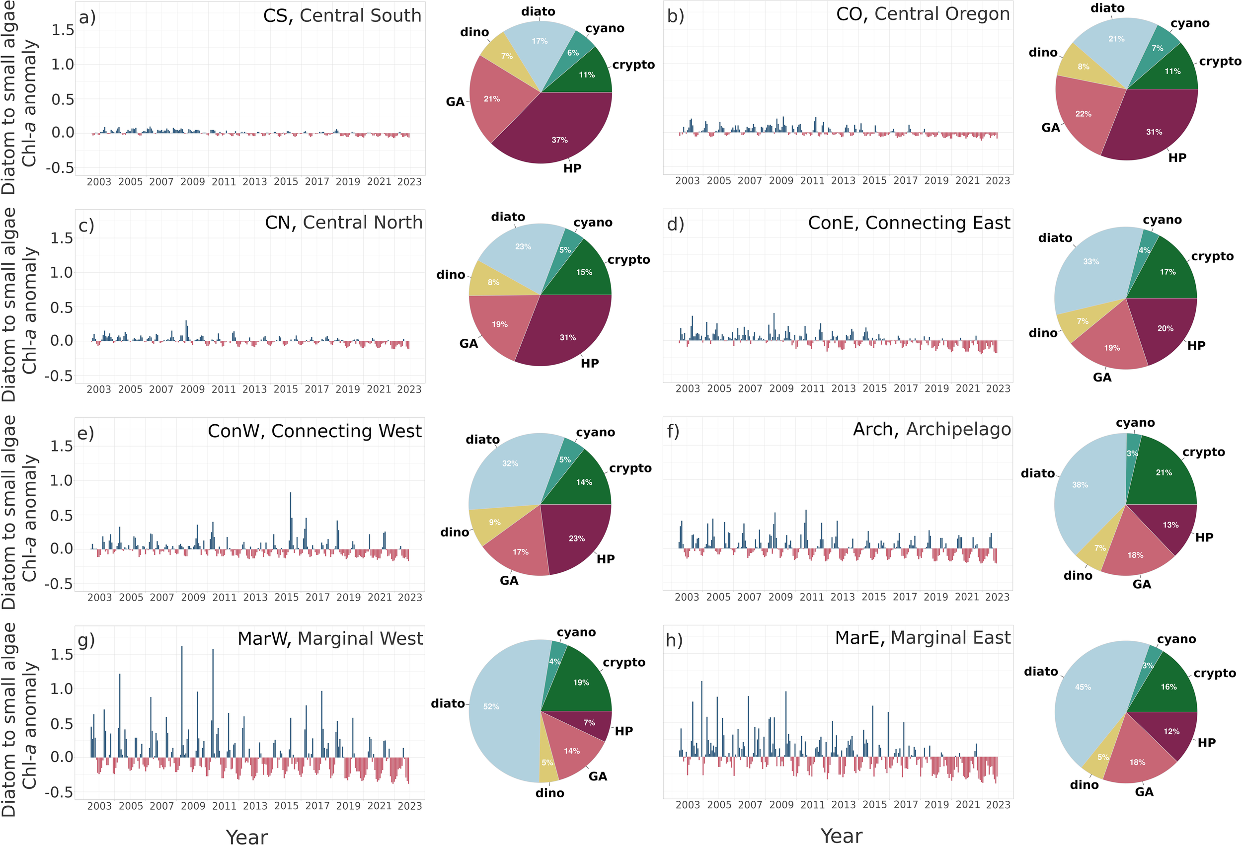
Anomaly for the period 2002–2022 of the proportion between the diatoms to the sum of the chlorophyll-a input from haptophytes, pelagophytes, green algae, and cyanobacteria within bioregions: (a) Central South, (b) Central Oregon, (c) Central North, (d) Connecting East, (e) Connecting West, (f) Archipelago, (g) Marginal West, (h) Marginal East, and the respective phytoplankton composition within each bioregion determined based on the Cmax climatology in the years 2002 – 2022.
Comparable results were obtained from the diatom-to-dinoflagellate ratio anomalies (Figure 6), where the negative anomalies in the last five years were evident across all bioregions. Moreover, a similar match in time between the shift towards the predominance of the negative diatom-to-dinoflagellate ratio anomalies (Figure 6) and the TotBLen decrease (Figure 3) was observed, such as a change in 2014 in ConE and MarE (Figures 3d, h, 6d, h), and in 2018 in ConW (Figures 3e, 6e).
Figure 6
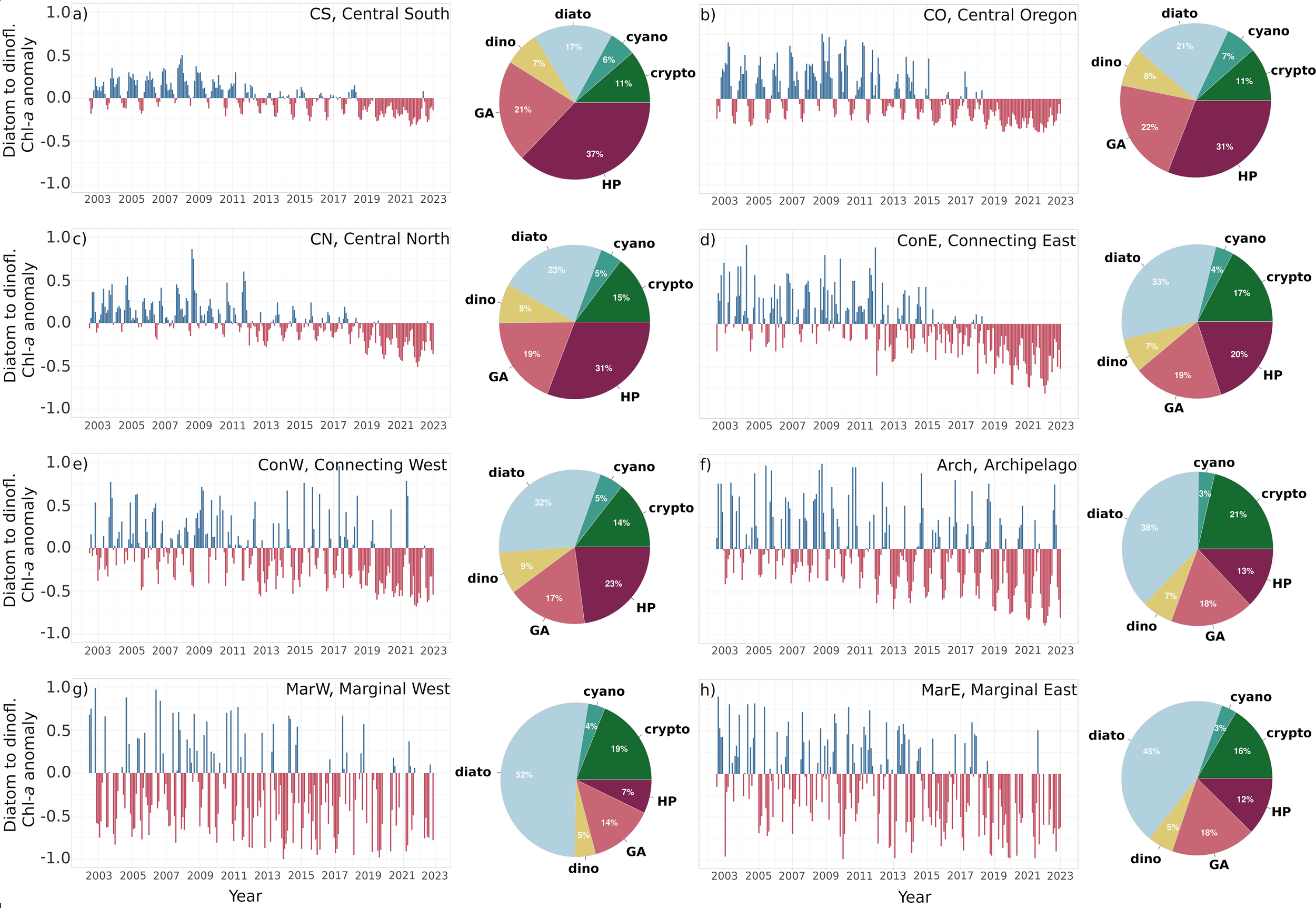
Diatom-to-dinoflagellate chlorophyll-a ratio anomaly in the years 2002–2022 within bioregions: (a) Central South, (b) Central Oregon, (c) Central North, (d) Connecting East, (e) Connecting West, (f) Archipelago, (g) Marginal West, (h) Marginal East, and the respective phytoplankton composition within each bioregion determined based on the Cmax climatology in the years 2002 – 2022.
3.3 Environmental factor analysis
Regarding the environmental drivers, there were clear differences between the bioregions (Supplementary Figures S2–S7). In the central bioregions, CS, CO, CN, and ConW, the spring and summer SSH variability was the primary descriptor of the Chl-a seasonal change. Of secondary importance was the spring salinity change in bioregions CO and ConW, suggesting two distinct water mass mixing (Figures 7b, d), and in CS and CN, summer and fall SST and PAR influence was more pronounced (Figures 7a, c). The MarE and ConE bioregions, bordering the Gulf of Alaska, were influenced mainly by the winter and spring SST changes, followed by the winter MLD, spring and summer SST, and SSH variability (Figures 7e, h). The MarW bioregion was most impacted by the salinity fluctuations and SSH in spring and summer (Figure 7g). In contrast, Arch was the only bioregion where the summer CurrS was an important factor (Figure 7f), supported by the summer SST and SSH variability.
Figure 7
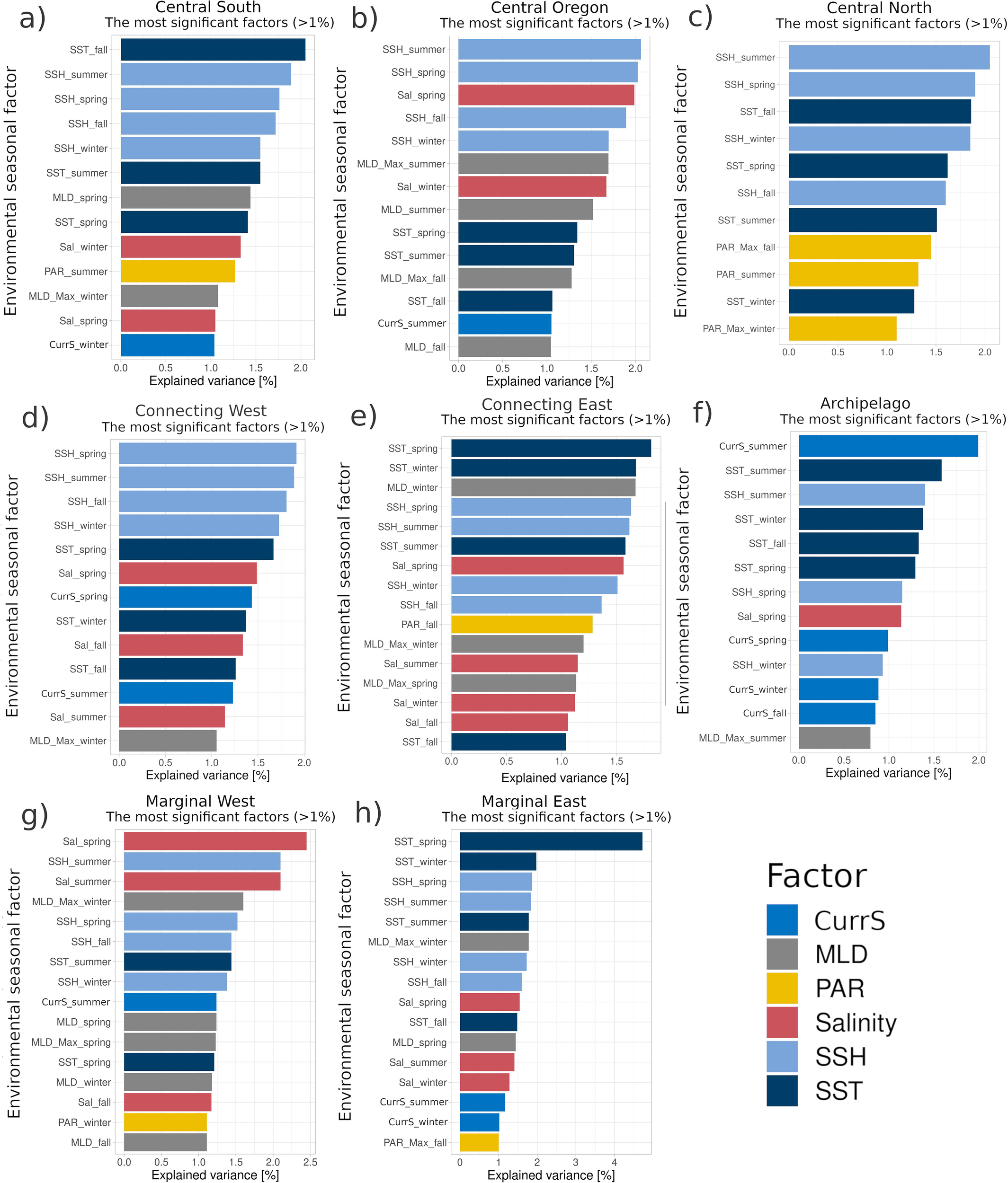
The key environmental factors characterizing seasonal variability (winter: January – March, spring: April – June, summer: July – September, and fall: October – December) within the bioregions: (a) Central South (CS), (b) Central Oregon (CO), (c) Central North (CN), (d) Connecting East (ConE), (e) Connecting West (ConW), (f) Archipelago (Arch), (g) Marginal West (MarW), (h) Marginal East (MarE), determined using the Multiple Factor Analysis (MFA).
3.4 Climate indices analysis
Considering the climate indices (Figure 8), the global ENSO pattern represented here by the MEI v2 indicated El Niño (MEI>1.5) in 1998, 2009/2010, and 2015/2016, and La Niña (MEI<1.5) in the years 1999 – 2000, 2007 – 2009, 2010 – 2012, and 2020 – 2022. There was also a shift to the negative NPGO at the beginning of 2014, which remained negative until 2022, except for a few months in 2014 and 2016. The NPGO and the PDO did not correlate during the analyzed period (Supplementary Figure S1), where the negative PDO was observed in the years 2008 – 2009, 2010 – 2014, and 2020 – 2022.
Figure 8

Monthly changes of the leading climate indices, including (a) the Multivariate El Niño–Southern Oscillation index (MEIv2; Zhang et al., 2019), (b) the North Pacific Gyre Oscillation (NPGO, Di Lorenzo et al., 2008), (c) the Pacific Decadal Oscillation (PDO, Bond and Harrison, 2000), (d) the Pacific–North America (PNA) pattern (Wallace and Gutzler, 1981), and (e) the North Pacific Index anomaly in the years 1998 – 2022 (NPI, Trenberth and Hurrell, 1994).
The statistical results based on the Mann-Kendall test generally revealed three main patterns: (1) the large impact of the NPGO on the bloom phenology in the central CO and CN and the eastern ConE and MarE bioregions (Table 2), (2) the strong influence of the El Niño-Southern Oscillation (ENSO—MEI v2) on the south-central CS and CO, and (3) the primary role of the Aleutian Low on the western part of the Pacific, including the ConW, MarW, and Arch, which was reflected in significant relationships between the phenology metrics, especially SLen and BLen, and the NPI, the ALBSA, and the PNA.
Table 2
| Phenology metric | CS | CO | CN | ConE | ConW | MarE | MarW | Arch | ||||||||
|---|---|---|---|---|---|---|---|---|---|---|---|---|---|---|---|---|
| + | - | + | - | + | - | + | - | + | - | + | - | + | - | + | - | |
| Cmax | SOI | NPGO | PNA sAO | NPI | sAO | sAO | sAO | sAO | ||||||||
| FBstart | wAO NPI | wAO | NPI | ALBSA | ||||||||||||
| TotBLen | NPGO | NPGO | wAO NPI | NPGO | MEIv2 PDO | |||||||||||
| Bmagn | NPGO | PNA sAO | NPI | sAO | sAO | sAO | sAO | |||||||||
| Bstart | NPI | SOI | ||||||||||||||
| SLen | NPGO | wAO NPI | NPGO | NPI | PNA NPGO | ALBSA NPI | sAO | NPGO | wAO ALBSA NPI | PNA NPGO | NPI ALBSA | |||||
| BLen | NPGO | PDO MEIv2 | NPGO | NPGO | PNA | ALBSA NPI | NPGO | sAO | ||||||||
| Summary | wAO | NPGO | NPGO, wAO, sAO, NPI | NPGO, sAO | PNA, NPI | NPGO, sAO | ALBSA, sAO | sAO, NPI | ||||||||
Climate indices* significantly correlated with the yearly changes in the phytoplankton phenology metrics within bioregions: Central South (CS), Central Oregon (CO), Central North (CN), Connecting East (ConE), Connecting West (ConW), Marignal East (MarE), Marginal West (MarW), and Archipelago (Arch), determined using the non-parametric Mann-Kendall test.
Plus sign indicates a proportional and minus an inversely proportional relationship, where p<0.05, and in bold were marked cases where p<0.01. Only statistically significant (p<0.05) values were included here. Note that the bottom row (Summary) summarizes the key indices impacting the phenology metrics in each bioregion.
*The indices are as follows: the Southern Oscillation Index (SOI) (Trenberth, 1984); the Multivariate El Niño–Southern Oscillation index (MEIv2) (Zhang et al., 2019); the Arctic Oscillation index (wAO in winter Nov–April; Thompson and Wallace, 1998, and sAO in summer July–Sept) (Ogi and Wallace, 2007); the Pacific–North America (PNA) pattern (Wallace and Gutzler, 1981); the North Pacific Index (NPI) (Trenberth and Hurrell, 1994); the Pacific Decadal Oscillation (PDO) (Bond and Harrison, 2000); the North Pacific Gyre Oscillation (NPGO) (Di Lorenzo et al., 2008); the Aleutian Low‐Beaufort Sea Anticyclone (ALBSA) (Cox et al., 2019).Each color corresponds to a specific bioregion, as introduced in Figure 2.
4 Discussion
This study analyzed changes in the phytoplankton phenology and composition from 2002 to 2022 and the potential drivers in bioregions within the subarctic Pacific Ocean. The changepoint analysis showed a regime shift in the last two decades towards shorter total bloom length (TotBLen) in most bioregions, except for the MarW (Figure 3g). In the bordering Gulf of Alaska (GoA), bioregions ConE and MarE, TotBLen decreased by a month (Figures 3d, h). These decreases corresponded with a gradual reduction in the ratio of diatom-to-small-cell phytoplankton and diatom-to-dinoflagellates. This ratio change may explain the decrease in TotBLen, as diatoms are the main group forming spring blooms and a large contributor to total Chl-a in the subarctic Pacific region (Obayashi et al., 2001), discussed further below. Additionally, we analyzed the relationships between environmental factors and Chl-a variability, and climate indices and phenology metrics to interpret potential climatic causes of the observed changes in phenology and phytoplankton composition.
4.1 Change in the phytoplankton composition
Our study revealed a general decrease between 2002 and 2022 in the diatom to small-cell phytoplankton Chl-a ratio anomaly (Figure 5) and the diatom to dinoflagellates Chl-a ratio anomaly (Figure 6). The decreasing trend was statistically significant in all bioregions, but the most pronounced anomalies were observed in the connecting and marginal bioregions, ConE and MarE (Figures 5d, h), where the biggest changes in the TotBLen were also observed (Figures 3d, h). A decrease in bloom-forming diatom contribution and a shift towards smaller phytoplankton could dampen the annual Chl-a variability and likely cause a change in the observed TotBLen. Previous phytoplankton composition analyses in the years 2012–2015 in the GoA and its margin suggested a drop in diatom production and a shift towards smaller phytoplankton groups, such as haptophytes, chlorophytes, and cyanobacteria, mainly during the marine heat wave (MHW) periods (Peña et al., 2019; Taves et al., 2022). The major MHW in the Northeast Pacific, where we observed the most significant change in diatom input, were the ones during the winters of 2013/14 (Bond et al., 2015) and 2014/15 (Di Lorenzo and Mantua, 2016), and summer 2014 and 2019 (Amaya et al., 2020; Song et al., 2023). Lower diatom abundance during the MHW, between 2014 and 2016, was noticed in the Continuous Plankton Recorder (CPRs) measurements in the GoA, among all measurements collected in the years 2000 – 2018 (Batten et al., 2022). Cael et al. (2021) also found the large-cell diatoms and dinoflagellates to be one of the most likely to experience an abrupt shift in biomass in the 2020s, and the more recent models confirmed a significant switch in community composition from diatoms to dinoflagellates in the Pacific (Arteaga and Rousseaux, 2023).
Our findings suggest that the reduction in diatom abundance in the northeast subarctic Pacific is not only a temporary effect of MHW, but may be part of a gradual change in the phytoplankton communities, confirming previous predictions of a decline in the diatom biomass (Boyd et al., 2004; Rousseaux and Gregg, 2015). Consequently, in the eastern bioregions with the highest contribution of diatoms, ConE and MarE, we observed the biggest change towards shorter TotBLen, which may impact the total primary production in the high latitudes of the subarctic Pacific Ocean (Tréguer et al., 2018). It is also important to stress that even a relatively small change in the diatom biomass can have a significant impact on marine export production (Waite et al., 1992) since they are responsible for roughly 40% of the particulate organic carbon export globally due to their fast-sinking silicate frustules and fecal pellets, resulting from the intense diatom grazing in the higher latitudes (> 50°N) (Jin et al., 2006).
4.2 Climate indices, environmental factors, and phytoplankton phenology
The NPGO index has been widely recognized as strongly linked to the oceanographic conditions in the eastern subarctic Pacific since it describes the water flow intensity in the eastern and central branches of the North Pacific Gyres (Stramma et al., 2020). Here, we observed a positive relationship between the NPGO and the BLen in the eastern bioregions ConE and MarE, and the TotBLen in the central bioregions CO and CN (Table 2). These positive relationships are likely associated with increased nutrient availability in the GoA region and the California Current System during positive NPGO regimes (Di Lorenzo et al., 2008). For these bioregions, the influence of the PDO was of secondary importance, which contrasts with the findings of Bond and Harrison (2000), who identified the PDO as a primary factor impacting the North Pacific. Recent studies have also reported a weaker impact of the PDO on the eastern North Pacific ecosystems (Kilduff et al., 2015; Litzow et al., 2018). The positive PDO phase is typically associated with above-average water temperatures in the eastern subarctic Pacific and cooler-than-average temperatures in the western part (Graham et al., 2021). However, in our study, the PDO was primarily correlated with the TotBLen in the ConW bioregion, located in the Kuroshio bifurcation zone (Table 2). One potential reason for the relationship between BLen and the NPGO, instead of the PDO, is that both PDO and NPGO are influenced by El Niño events, albeit in different ways. Kilduff et al. (2015) noted changes in contemporary El Niño events, suggesting that recent El Niño occurrences are more frequently associated with central Pacific warming, which indirectly modulates the NPGO rather than causing the eastern Pacific warming that regulates the PDO. During the period covered in this paper (2002 – 2022), the relationship between the PDO and the NPGO was not statistically significant (Supplementary Figure S1), confirming the difference in how the two are modulated.
Our findings also showed a direct impact of the ENSO pattern on BLen in the CO bioregion and Cmax in CS, whereas in the western bioregions, ConW, MarW, and Arch, SLen and BLen were more related to the NPI, the PNA, and the ALBSA indices (Table 2). Some degree of intercorrelation between these three indices was observed: proportional between the NPI and the ALBSA and inversely proportional between the PNA and the ALBSA (Supplementary Figure S1). Nonetheless, all three were included in the analysis because they have been widely discussed in the literature as part of a global teleconnection network (Schwing et al., 2010) and were shown to better describe various aspects of the natural variability related to the Aleutian Low together, especially when combined with the AO, than when used separately (Overland et al., 1999). The Aleutian Low — represented by the NPI — affected all the western bioregions, including the Arch, MarW, ConW, and CN. However, the SLen in the MarW bioregion, bordering the Kamchatka Peninsula, was influenced primarily by the ALBSA index, characterizing the ice melt in the Bering Sea region (Cox et al., 2019). Additionally, the relationship between the ALBSA and the AO, which is known to control the sea ice melt in the Okhotsk Sea, the snow melts, and the Amur River discharge around the Kamchatka Peninsula (Tachibana et al., 2008), indicates the critical role of the land runoff in the western Subarctic Pacific (Ogi and Tachibana, 2006), which was reflected in statistically significant relationships with SLen and BLen in the ConW, MarW, and Arch bioregions. These relationships confirm the primary role of salinity among the environmental factors (Figure 7g), which is unique to the MarW bioregion. Moreover, the Amur River carries exceptionally high loads of iron (Shamov et al., 2014), likely reflected in the highest observed Chl-a in MarW among all the bioregions (Figure 4b).
The Aleutian Low, captured by the NPI and PNA indices, also affected ConW and CN bioregions (Table 2). Particularly in the ConW, located in the Kuroshio Bifurcation zone, the PNA influence on SLen and BLen was marked, which may be related to the higher frequency of tropical cyclone occurrence in the Kuroshio region (Song and Klotzbach, 2019), reflected in the SSH and SST variability (Figure 7d). In the neighboring Arch bioregion, SLen was also impacted by the NPI, in addition to the PNA and the ALBSA indices. Still, the main factors in this bioregion were the CurrS and SST in summer (Figure 7f), suggesting the primary role of the ocean currents (Abe and Nakamura, 2013; Nishioka et al., 2020). Positive SLen correlation with the NPGO indicates that the stronger mixing within the gyre likely introduces more nutrients to sustain longer blooms. The negative correlation with the NPI, on the other hand, suggests that stronger storms and diapycnal mixing may weaken water column stratification and lead to deepening of the mixed layer (Suga et al., 2004) below the critical depth described by Sverdrup’s theory (Smetacek and Passow, 1990), and resulting in shorter SLen. Lastly, the NPI and the AO influence on FBstart, SLen, and TotBLen was also noticed in the two largest bioregions, CN and CS (Table 2). These bioregions are governed by the Aleutian Low, controlling the strength of the westerly winds and the wind-related stress over the North Pacific (Goes et al., 2004), which affects the mixed layer depth and the transport of Fe-rich dust from Asian deserts (Duce and Tindale, 1991), especially to the mid-latitudes (between 35° and 45°N). The key factors in the central subarctic Pacific were the SSH and PAR (Figure 7c), providing more nutrients and light to sustain primary productivity, which also agreed with the general patterns described by Goes et al. (2004).
Summary characteristics of each bioregion’s dominant environmental factors and climate indices were compiled in Table 3.
Table 3
| Bioregion | Characteristic features | |
|---|---|---|
| Central South (CS) | The southernmost bioregion with the lowest Chl-a concentrations with irregular phenology patterns controlled by the SSH and short-term weak vertical mixing, with the largest share of haptophytes and pelagophytes of all bioregions due to adjacent transitional and tropical water influx reflected in correlation with the SST; biological variability related to the large-scale SOI index and the strength of the Aleutian Low captured by the NPI index. | |
| Central Oregon (CO) | The relatively small bioregion off the coast of California, USA, overlapping spatially with the split of the North Pacific Current, which is reflected in the strong imprint of SSH and salinity on the phytoplankton variability, domination by small algae, and strong correlation with the NPGO index. | |
| Central North (CN) | The central subarctic Pacific bioregion is dominated by small algae, related to the SSH and large-scale mixing within the Subarctic Pacific Gyre, which is reflected in the correlation with the NPGO index. | |
| Connecting East (ConE) | The bioregion bordering the Gulf of Alaska, between the CN and MarE, is strongly influenced by SST and the MLD in winter/spring; its correlation with the NPGO index indicates a strong influence of gyre-related mixing, and its summer dependence on the SSH suggests the influence of eddy activity; a decrease of diatoms after 2014 has been apparent. | |
| Connecting West (ConW) | This bioregion is located where the warm and salty Kuroshio and the cold and fresher Oyashio waters mix, controlled by SSH fluctuations and changes in the salinity and SST, resulting from the intense eddy activity in this region; significantly influenced by the Aleutian Low’s strength, characterized by the NPI and PNA indices, likely related to the number of tropical cyclones; some decrease in the diatoms after 2018 was observed, but less pronounced than in the east. | |
| Marginal East (MarE) | The bioregion close to continental slope with the highest Chl-a concentrations and the evident drop in diatoms after 2014, which co-occurs in time with the TotBLen decrease; strongly related to the SST and SSH changes, which underlines the importance of eddy activity and correlates with the NPGO and SOI indices. | |
| Marginal West (MarW) | The bioregion in the western Pacific, offshore of the coast of Japan and Russia, defined by the changes in salinity; strong influence of the meltwater from the Okhotsk Sea, the Bering Sea, and the Kamchatka Peninsula, confirmed by the correlation with ALBSA index, characterizing start of the melting time in the Bering Sea region, revealing the primary role of the Fe input in controlling SLen in this region; the only bioregion where TotBLen increased (in 2001). | |
| Archipelago (Arch) | The island-bordered bioregion, located along the Kuril and the Aleutian Archipelagos, where the CurrS and SST are the main drivers, indicating high importance of tidal mixing with the adjacent seas, rather than the eddy/gyre mixing related to the SSH; controlled by the strength of the Aleutian Low, captured by the NPI index. | |
Summarized bioregion characteristics.
Each color corresponds to a specific bioregion, as introduced in Figure 2.
4.3 Importance for the ecosystem
Changes in the length of the TotBLen and diatom contribution will likely affect the entire ecosystem through impacts on zooplankton production, community composition and nutritional quality (Suchy et al., 2022; McLaskey et al., 2024). At a higher trophic level, Piatt et al. (2020) reported high mortality and reproductive failure of common murres (Uria aalge) in the years 2014–2016 linked to the abnormally low phytoplankton biomass and shift in the zooplankton community structure toward less-nutritious taxa. Nielsen et al. (2021) also revealed a significant change in the composition of the ichthyoplankton assemblages during the MHW along the GoA shelf. Nonetheless, the full picture may be more complicated, with Batten et al. (2022) not finding lower zooplankton abundance overall in the GoA during the 2014–2016 MHW, even though a decrease in the diatom-to-small algae ratio was reported. Although before the MHW in 2014, SST had been positively correlated with the abundance of diatoms and zooplankton biomass, during the MHW, zooplankton biomass did not follow the drop in diatom abundance (Batten et al., 2022). On the contrary, the high numbers of zooplankton, with the higher metabolic rates boosted by the elevated SST, were hypothesized to increase the grazing pressure on diatoms. The declines in cold-water zooplankton taxa and general species richness were also noted, indicating that the phytoplankton and zooplankton community structure shift is more probable than a drop in their biomass.
The positive correlation between NPGO and the phytoplankton phenology metrics, particularly BLen in the eastern bioregions, MarE and ConE (Table 2), supports recent research showing a change toward a more pronounced impact of the NPGO on the west coast of North America (Kilduff et al., 2015; Puerta et al., 2019; Suchy et al., 2022) compared to the PDO which has been historically associated with variability of Pacific salmon (Mantua et al., 1997). Furthermore, recently the NPGO combined with the SOI has been shown to be strongly correlated with the recruitment abundance of Japanese sardine (Sardinops melanostictus) in the Kurosio — Oyashio Extension (Yatsu et al., 2021) of the western North Pacific.
All the above findings show certain changes in the food web structure, which appear to be associated mainly with the MHW period. However, the expected increasing frequency of MHW (Song et al., 2023) may change biological landscape permanently in the near future, and the NPGO might be a better predictor of the environmental variability directly affecting the food web in the subarctic Pacific.
5 Conclusions
This study aimed at investigating long-term changes in phytoplankton phenology and composition, as well as determining the main drivers of phytoplankton variability. To achieve this goal, we derived phytoplankton phenology metrics and phytoplankton functional types in the years 2002–2022 from the GlobColour satellite data series over the subarctic Pacific Ocean. Our findings indicate a decrease in the total length of phytoplankton blooms in recent years throughout most bioregions, except for the waters surrounding the Kamchatka Peninsula, represented by bioregion MarW. In the regions bordering the Gulf of Alaska, represented by bioregions MarE and ConE, we documented a reduction of one month in the total length of phytoplankton blooms post-2014, after the first of the two severe marine heatwaves in this region. Furthermore, we identified a decreasing trend throughout the analyzed period in both the diatom-to-dinoflagellate ratio anomaly and the diatom-to-small algae ratio anomaly, consisting of haptophytes, pelagophytes, green algae, and cyanobacteria. A sharp diatom decline was particularly pronounced in the Gulf of Alaska after 2018, suggesting a significant shift in phytoplankton community structure. To pinpoint the main factors influencing phytoplankton dynamics within each bioregion, we compared Chl-a concentrations with hydrological conditions and phytoplankton phenology and composition with climate indices. Our analysis linked the decline in diatom populations and the overall reduction in bloom length with the decreased intensity of oceanic circulation within the Subarctic Pacific Gyre, represented by the negative NPGO index. Our bioregion-focused approach proved highly effective, revealing the distinct driving mechanisms operating across different regions of the subarctic Pacific Ocean. Gaining a comprehensive understanding of these mechanisms is critical for making accurate predictions about future trends and for effectively adjusting marine management strategies to ensure the sustainability of these vital marine ecosystems.
Statements
Data availability statement
The raw data supporting the conclusions of this article will be made available by the authors, without undue reservation.
Author contributions
MK: Formal Analysis, Writing – review & editing, Data curation, Writing – original draft, Methodology, Investigation, Visualization, Validation, Conceptualization. BH: Writing – review & editing, Methodology, Conceptualization, Supervision. MP: Methodology, Writing – review & editing, Conceptualization, Supervision. TH: Supervision, Conceptualization, Writing – review & editing, Methodology. CM: Methodology, Writing – review & editing. PV: Writing – review & editing, Methodology. AB: Writing – review & editing, Methodology. HX: Methodology, Writing – review & editing, Funding acquisition. MC: Supervision, Project administration, Funding acquisition, Methodology, Software, Resources, Conceptualization, Writing – review & editing.
Funding
The author(s) declare that financial support was received for the research and/or publication of this article. The work was funded by the British Columbia Salmon Restoration and Innovation Fund (BCSRIF) through the North Pacific Anadromous Fish Commission -the International Year of the Salmon Secretariat and NSERC Discovery Grant to Costa. Contributions by HX and AB were funded by the Copernicus Marine Service Evolution project GLOPHYTS (21036L05B-COP-INNO SCI-9000).
Acknowledgments
We thank the colleagues and the crews of R/V Sir John Franklin, R/V Bell M. Shimada, and R/V TINRO for collecting the in situ samples during the International Year of the Salmon High-Seas Expedition (Weitkamp et al., 2024). This study has been conducted using E.U. Copernicus Marine Service Information: https://doi.org/10.48670/moi-00099 and GlobColour data (https://hermes.acri.fr/index.php) developed, validated, and distributed by ACRI-ST, France. Data from the monitoring stations along Line-P were available thanks to the courtesy of the Fisheries and Oceans Canada (https://open.canada.ca/data/en/dataset/8c630c40-a40f-42be-b5e1-e7ade5d560e5). The R scripts for the EOF based PFT retrieval models were adapted based on the original version developed by Marc Taylor.
Conflict of interest
The authors declare that the research was conducted in the absence of any commercial or financial relationships that could be construed as a potential conflict of interest.
Generative AI statement
The author(s) declare that no Generative AI was used in the creation of this manuscript.
Publisher’s note
All claims expressed in this article are solely those of the authors and do not necessarily represent those of their affiliated organizations, or those of the publisher, the editors and the reviewers. Any product that may be evaluated in this article, or claim that may be made by its manufacturer, is not guaranteed or endorsed by the publisher.
Supplementary material
The Supplementary Material for this article can be found online at: https://www.frontiersin.org/articles/10.3389/fmars.2025.1609094/full#supplementary-material
References
1
Abe S. Nakamura T. (2013). Processes of breaking of large-amplitude unsteady lee waves leading to turbulence. J. Geophysical Research: Oceans118, 316–331. doi: 10.1029/2012JC008160
2
Alvain S. Moulin C. Dandonneau Y. Bréon F. M. (2005). Remote sensing of phytoplankton groups in case 1 waters from global SeaWiFS imagery. Deep-Sea Res. I52, 1989–2004. doi: 10.1016/j.dsr.2005.06.015
3
Amaya D. Miller A. J. Xie S.-P. Kosaka Y. (2020). Physical drivers of the summer 2019 North Pacific marine heatwave. Nat. Commun.11, 1903. doi: 10.1038/s41467-020-15820-w
4
Arteaga L. A. Rousseaux C. S. (2023). Impact of Pacific Ocean heatwaves on phytoplankton community composition. Commun. Biol.6, 263. doi: 10.1038/s42003-023-04645-0
5
Auguie B. Antonov A. (2017). Miscellaneous Functions for ``Grid’’ Graphics. R package version 2.3. doi: 10.32614/CRAN.package.gridExtra
6
Batten S. D. Ostle C. Hélaouët P. Walne A. W. (2022). Responses of Gulf of Alaska plankton communities to a marine heat wave. Deep-Sea Res. Part II195, 105002. doi: 10.1016/j.dsr2.2021.105002
7
Bond N. A. Cronin M. F. Freeland H. Mantua N. (2015). Causes and impacts of the 2014 warm anomaly in the NE Pacific. Geophysical Res. Lett.42, 3414–3420. doi: 10.1002/2015GL063306
8
Bond N. A. Harrison D. E. (2000). The Pacific Decadal Oscillation, air–sea interaction and central north Pacific winter atmospheric regimes. Geophysical Res. Lett.27, 731–734. doi: 10.1029/1999GL010847
9
Boyce D. Lewis M. Worm B. (2010). Global phytoplankton decline over the past century. Nature466, 591–596. doi: 10.1038/nature09268
10
Boyd P. Law C. Wong C. Nojiri Y. Tsuda A. Levasseur M. et al . (2004). The decline and fate of an iron-induced subarctic phytoplankton bloom. Nature428, 549–555. doi: 10.1038/nature02437
11
Bracher A. Bouman H. A. Brewin R. J. W. Bricaud A. Brotas V. Ciotti A. M. et al . (2017). Obtaining phytoplankton diversity from ocean color: A scientific roadmap for future development. Front. Mar. Sci.4. doi: 10.3389/fmars.2017.00055
12
Brody S. R. Lozier M. S. Dunne J. P. (2013). A comparison of methods to determine phytoplankton bloom initiation. J. Geophysical Research: Oceans118, 2345–2357. doi: 10.1002/jgrc.20167
13
Cael B. B. Dutkiewicz S. Henson S. (2021). Abrupt shifts in 21st-century plankton communities. Sci. Adv.7, eabf8593. doi: 10.1126/sciadv.abf8593
14
Capotondi A. Alexander M. A. Deser C. Miller A. J. (2005). Low-frequency pycnocline variability in the northeast Pacific. J. Phys. Oceanography35, 1403–1420. doi: 10.1175/JPO2757.1
15
Chiba S. Batten S. D. Yoshiki T. Sasaki Y. Sasaoka K. Sugisaki H. et al . (2015). Temperature and zooplankton size structure: climate control and basin-scale comparison in the North Pacific. Ecol. Evol.5, 968–978. doi: 10.1002/ece3.1408
16
Clemons M. J. Miller C. B. (1984). Blooms of large diatoms in the oceanic, subarctic Pacific. Deep Sea Res. Part A. Oceanographic Res. Papers31, 85–95. doi: 10.1016/0198-0149(84)90076-1
17
Cox C. J. Stone R. S. Douglas D. C. Stanitski D. M. Gallagher M. R. (2019). The Aleutian Low-Beaufort Sea Anticyclone: A climate index correlated with the timing of springtime melt in the Pacific Arctic cryosphere. Geophysical Res. Lett.46, 7464–7473. doi: 10.1029/2019GL083306
18
Crusius J. (2021). Dissolved Fe supply to the central Gulf of Alaska is inferred to be derived from Alaskan glacial dust that is not resolved by dust transport models. J. Geophysical Research: Biogeosciences126, e2021JG006323. doi: 10.1029/2021JG006323
19
Crusius J. Schroth A. W. Resing J. A. Cullen J. Campbell R. W. (2017). Seasonal and spatial variabilities in northern Gulf of Alaska surface water iron concentrations driven by shelf sediment resuspension, glacial meltwater, a Yakutat eddy, and dust. Global Biogeochemical Cycles31, 942–960. doi: 10.1002/2016GB005493
20
Cushing D. H. (1990). Plankton production and year-class strength in fish populations: an update of the match/mismatch hypothesis. Adv. Mar. Biol.26, 249–293. doi: 10.1016/S0065-28810860202-3
21
Davis K. A. Banas N. S. Giddings S. N. Siedlecki S. A. MacCready P. Lessard E. J. et al . (2014). Estuary-enhanced upwelling of marine nutrients fuels coastal productivity in the U.S. Pacific Northwest. J. Geophysical Research: Oceans119, 8778–8799. doi: 10.1002/2014JC010248
22
Di Lorenzo E. Mantua N. (2016). Multi-year persistence of the 2014/15 North Pacific marine heatwave. Nat. Climate Change6, 1042–1047. doi: 10.1038/nclimate3082
23
Di Lorenzo E. Schneider N. Cobb K. M. Franks P. J. S. Chhak K. Miller A. J. et al . (2008). North Pacific Gyre Oscillation links ocean climate and ecosystem change. Geophysical Res. Lett.35, L08607. doi: 10.1029/2007GL032838
24
Doney S. C. Ruckelshaus M. Duffy J. E. Barry J. P. Chan F. English C. A. et al (2012). Climate Change Impacts on Marine Ecosystems. Annual Reviews of Marine Science4, 11–37. doi: 10.1146/annurev-marine-041911-111611
25
Duce R. A. Tindale N. W. (1991). Atmospheric transport of iron and its deposition in the ocean. Limnology Oceanography36, e2020JC017127. doi: 10.4319/lo.1991.36.8.1715
26
Eisner L. B. Lomas M. W. (2022). Data from: Flow cytometry data from the R/V TINRO, NOAA Bell M. Shimada and CCGS Sir John Franklin during the 2022 International Year of the Salmon Pan-Pacific Winter High Seas Expedition. North Pacific Anadromous Fish Commission. doi: 10.21966/j26w-by50
27
Falkowski P. G. Katz M. E. Knoll A. H. Quigg A. Raven J. A. Schofield O. et al (2004). The evolution of modern eukaryotic phytoplankton. Science305, 354–360. doi: 10.1126/science.1095964
28
Fiechter J. Moore A. M. Edwards C. A. Bruland K. W. Di Lorenzo E. Lewis C. V. W. et al (2009). Modeling iron limitation of primary production in the coastal Gulf of Alaska. Deep-Sea Research: II56, 2503–19. doi: 10.1016/j.dsr2.2009.02.010
29
Frölicher T. L. Laufkötter C. (2018). Emerging risks from marine heat waves. Nat. Commun.9, 650. doi: 10.1038/s41467-018-03163-6
30
Frouin R. McPherson J. Ueyoshi K. Franz B. A. (2012). A time series of photosynthetically available radiation at the ocean surface from SeaWiFS and MODIS data. Remote Sens. Mar. Environ. II. 8525, 852519. doi: 10.1117/12.981264
31
Fukuwaka M. Ishida Y. Michida Y. Sugimoto S. Tadokoro K. Watanuki Y. et al . (2004). “Western subarctic gyre,” in Marine Ecosystems of the North Pacific. Eds. PerryR. I.McKinnellS. M. (Canada: PICES), 129–139.
32
Gargett A. E. (1991). Physical processes and the maintenance of nutrient-rich euphotic zones. Limnology Oceanography36, 1527–1545. doi: 10.4319/lo.1991.36.8.1527
33
Gaube P. Chelton D. B. Samelson R. M. Schlax M. G. O’Neill L. W. (2015). Satellite observations of mesoscale eddy-induced Ekman pumping. J. Phys. Oceanography45, 104–132. doi: 10.1175/JPO-D-14-0032.1
34
Glibert P.M. Burford M.A. (2017). Globally changing nutrient loads and harmful algal blooms: Recent advances, new paradigms, and continuing challenges. Oceanography. 30 (1), 58–69. doi: 10.5670/oceanog.2017.110
35
Goes J. I. Sasaoka K. Gomes H. Saitoh S.-I. Saino T. (2004). A comparison of the seasonality and interannual variability of phytoplankton biomass and production in the western and eastern gyres of the subarctic pacific using multi-sensor satellite data. J. Oceanography60, 75–91. doi: 10.1023/B:JOCE.0000038320.94273.25
36
Graham C. Pakhomov E. A. Hunt B. P. V. (2021). Meta-analysis of salmon trophic ecology reveals spatial and interspecies dynamics across the North Pacific Ocean. Front. Mar. Sci.8. doi: 10.3389/fmars.2021.618884
37
Guinehut S. Dhomps A.-L. Larnicol G. Le Traon P.-Y. (2012). High resolution 3D temperature and salinity fields derived from in situ and satellite observations. Ocean Sci.8, 845–857. doi: 10.5194/os-8-845-2012
38
Hamme R. C. Webley P. W. Crawford W. R. Whitney F. A. DeGrandpre M. D. Emerson S. R. et al . (2010). Volcanic ash fuels anomalous plankton bloom in subarctic northeast Pacific. Geophysical Res. Lett.37, L19604.
39
Harris C. R. Millman K. J. van der Walt S. J. Gommers R. Virtanen P. Cournapeau D. et al . (2020). Array programming with numPy. Nature585, 357–362. doi: 10.1038/s41586-020-2649-2
40
Harrison P. J. (2002). Station papa time series: insights into ecosystem dynamics. J. Oceanography58, 259–264. doi: 10.1023/A:1015857624562
41
Harrison P. J. Boyd P. W. Varela D. E. Takeda S. Shiomoto A. Odate T. (1999). Comparison of factors controlling phytoplankton productivity in the NE and NW subarctic Pacific. Prog. Oceanography43, 205–234. doi: 10.1016/S0079-6611(99)00015-4
42
Harrison P. L. Whitney F. A. Tsuda A. Saito H. Tadokoro K. (2004). Nutrient and plankton dynamics in the NE and NW gyres of the subarctic Pacific Ocean. J. Oceanography60, 93–177. doi: 10.1023/B:JOCE.0000038321.57391.2a
43
Henson S. A. Cael B. B. Allen S. R. Dutkiewicz S. (2021). Future phytoplankton diversity in a changing climate. Nat. Commun.12, 5372. doi: 10.1038/s41467-021-25699-w
44
Hirsch R. M. Slack J. R. Smith R. A. (1982). Techniques of trend analysis for monthly water quality data. Water Resour. Res.18, 107–121. doi: 10.1029/WR018i001p00107
45
Hjort J. (1926). Fluctuations in the year classes of important food fishes. ICES J. Mar. Sci.1, 5–38. doi: 10.1093/icesjms/1.1.5
46
Hollander M. Wolfe D. A. (1973). Non-parametric Statistical Methods (New York: John Wiley & Sons), 185–194.
47
Huang B. Liu C. Banzon V. Freeman E. Graham G. Hankins B. et al . (2021). Improvements of the daily optimum interpolation sea surface temperature (DOISST) version 2.1. J. Climate34, 2923–2939. doi: 10.1175/JCLI-D-20-0166.1
48
Hunt B. P. V. Alin S. Bidlack A. Diefenderfer H. L. Jackson J. M. Kellogg C. T. E. et al . (2024). Advancing an integrated understanding of land–ocean connections in shaping the marine ecosystems of coastal temperate rainforest ecoregions. Limnology Oceanography69, 3061–3096. doi: 10.1002/lno.12724
49
Huot Y. Babin M. Bruyant F. Grob C. Twardowski M. S. Claustre H. (2007). Does chlorophyll a provide the best index of phytoplankton biomass for primary productivity studies? Biogeosciences Discussions4, 707–745. doi: 10.5194/bgd-4-707-2007
50
Irwin A. J. Finkel Z. V. Müller-Karger F. E. Ghinaglia L. T. (2015). Phytoplankton adapt to changing ocean environments. Proc. Natl. Acad. Sci.112, 5762–5766. doi: 10.1073/pnas.1414752112
51
Isles P. D. F. Pomati F. (2021). An operational framework for defining and forecasting phytoplankton blooms. Frontiers in Ecology and the Environment19, 443–50. doi: 10.1002/fee.2376
52
Itoh S. Yasuda I. (2010). Characteristics of mesoscale eddies in the Kuroshio–Oyashio extension region detected from the distribution of the sea surface height anomaly. J. Phys. Oceanography40, 1018–1034. doi: 10.1175/2009JPO4265.1
53
Jin X. Gruber N. Dunne J. P. Sarmiento J. L. Armstrong R. A. (2006). Diagnosing the contribution of phytoplankton functional groups to the production and export of particulate organic carbon, CaCO3, and opal from global nutrient and alkalinity distributions. Global Biogeochemical Cycles20, GB2015. doi: 10.1029/2005GB002532
54
Kassambara A. Mundt F. (2020). Factoextra: Extract and Visualize the Results of Multivariate Data Analyses. R Package Version 1.0.7. Available online at: https://CRAN.R-project.org/package=factoextra.
55
Kavanaugh M. T. Hales B. Saraceno M. Spitz Y. H. White A. E. Letelier R. M. (2014). Hierarchical and dynamic seascapes: A quantitative framework for scaling pelagic biogeochemistry and ecology. Prog. Oceanography120, 291–304. doi: 10.1016/j.pocean.2013.10.013
56
Kilduff D. P. Di Lorenzo E. Botsford L. W. Teo S. L. H. (2015). Changing central Pacific El Niños reduce stability of North American salmon survival rates. PNAS. 112 (35), 10962–10966. doi: 10.1073/pnas.1503190112
57
Killick R. Eckley I. A. (2014). “changepoint: An R Package for Changepoint Analysis.” J. Stat. Software58 (3), 1–19. doi: 10.18637/jss.v058.i03
58
Killick R. Fearnhead P. Eckley I. A. (2012). Optimal detection of changepoints with a linear computational cost. J. Am. Stat. Assoc.107, 1590–1598. doi: 10.1080/01621459.2012.737745
59
Killick R. Haynes H. Eckley I. (2022). Methods for Changepoint Detection. R package version 2.2.4. Available online at: https://CRAN.R-project.org/package=changepoint.
60
Konik M. Peña A. M. Hirawake T. Hunt B. P. V. Suseelan Vishnu P. Eisner L. B. et al . (2024). Bioregionalization of the subarctic Pacific based on phytoplankton phenology and composition. Prog. Oceanography. 228, 103315. doi: 10.1016/j.pocean.2024.103315
61
Krug L. A. Platt T. Sathyendranath S. Barbosa A. B. (2018). Patterns and drivers ofphytoplankton phenology off SW Iberia: A phenoregion based perspective. Prog. Oceanography. 165, 233–256. doi: 10.1016/j.pocean.2018.06.010
62
Lam P. J. Bishop J. K. B. (2008). The continental margin is a key source of iron to the HNLC North Pacific Ocean. Geophysical Res. Lett.35, L07608. doi: 10.1029/2008GL033294
63
Laufkötter C. Vogt M. Gruber N. (2013). Long-term trends in ocean plankton production and particle export between 1960–2006. Biogeosciences10, 7373–7393. doi: 10.5194/bg-10-7373-2013
64
Lavigne L. Civitarese G. Gačić M. D’Ortenzio F. (2018). Impact of decadal reversals of the north Ionian circulation on phytoplankton phenology. Biogeosciences15, 4431–4445. doi: 10.5194/bg-15-4431-2018
65
Le S. Josse J. Husson F. (2008). FactoMineR: an R package for multivariate analysis. J. Stat. Software25, 1–18. doi: 10.18637/jss.v025.i01
66
Litchman E. Edwards K. F. Klausmeier C. A. Thomas M. K. (2012). Phytoplankton niches, traits and eco-evolutionary responses to global environmental change. Mar. Ecol. Prog. Ser.470, 235–248. doi: 10.3354/meps09912
67
Litzow M. A. Ciannelli L. Puerta P. Wettstein J. J. Rykaczewski R. R. Opiekun M. (2018). Non-stationary climate – salmon relationships in the Gulf of Alaska. Proc. R. Soc. B285, 20181855. doi: 10.1098/rspb.2018.1855
68
Liu H. Chen M. Zhu F. Harrison P. J. (2016). Effect of diatom silica content on copepod grazing, growth and reproduction. Front. Mar. Sci.3. doi: 10.3389/fmars.2016.00089
69
Liu H. Suzuki K. Saito H. (2004). Community structure and dynamics of phytoplankton in the western subarctic Pacific ocean: A synthesis. J. Oceanography60, 119–137. doi: 10.1023/B:JOCE.0000038322.79644.36
70
Losa S. N. Soppa M. A. Dinter T. Wolanin A. Brewin R. J. W. Bricaud A. et al . (2017). Synergistic exploitation of hyper- and multi-spectral precursor sentinel measurements to determine phytoplankton functional types (SynSenPFT). Front. Mar. Sci.4. doi: 10.3389/fmars.2017.00203
71
Lourie S. A. Vincent A. C. J. (2004). Using biogeography to help set priorities in marine conservation. Conserv. Biol.18, 1004–1020. doi: 10.1111/j.1523-1739.2004.00137.x
72
Malick M. J. Cox S. P. Mueter F. J. Peterman R. M. (2015). Linking phytoplankton phenology to salmon productivity along a north–south gradient in the Northeast Pacific Ocean. Can. J. Fisheries Aquat. Sci.72, 697–708. doi: 10.1139/cjfas-2014-0298
73
Mantua N. J. Hare S. R. Zhang Y. Wallace J. M. Francis R. C. (1997). A pacific interdecadal climate oscillation with impacts on salmon production. Bull. Am. Meteorological Soc.78, 1069–1080. doi: 10.1175/1520-0477(1997)078<1069:APICOW>2.0.CO;2
74
Marchese C. Hunt B. P. V. Giannini F. Ehrler M. Costa M. (2022). Bioregionalization of the coastal and open oceans of British Columbia and Southeast Alaska based on Sentinel-3A satellite-derived phytoplankton seasonality. Front. Mar. Sci.9. doi: 10.3389/fmars.2022.968470
75
Martinez E. Antoine D. D’Ortenzio F. Gentili B. (2009). Climate-driven basin-scale decadal oscillations of oceanic phytoplankton. Science326, 1253–1256. doi: 10.1126/science.1177012
76
McKinney W. (2010). “Data structures for statistical computing in python,” in Proceedings of the 9th Python in Science Conference. Eds. van der WaltS.MillmanJ., 56–61. doi: 10.25080/Majora-92bf1922-00a
77
McLaskey A. K. Forster I. Hunt B. P. V. (2024). Distinct trophic ecologies of zooplankton size classes are maintained throughout the seasonal cycle. Oecologia204, 227–239. doi: 10.1007/s00442-023-05501-y
78
McLeod (2011). Kendall Rank Correlation and Mann-Kendall Trend Test. R package version 2.2.1.
79
Meyer M. G. Gong W. Kafrissen S. M. Torano O. Varela D. E. Santoro A. E. et al . (2022). Phytoplankton size-class contributions to new and regenerated production during the EXPORTS Northeast Pacific Ocean field deployment. Elementa: Sci. Anthropocene10, 68. doi: 10.1525/elementa.2021.00068
80
Millard S. P. (2013). EnvStats: An R Package for Environmental Statistics (New York: Springer).
81
Moisan T. A. Rufty K. M. Moisan J. R. Linkswiler M. A. (2017). Satellite observations of phytoplankton functional type spatial distributions, phenology, diversity, and ecotones. Front. Mar. Sci.4, 4189. doi: 10.3389/fmars.2017.00189
82
Mueter F. J. Batten S. D. Brickley P. J. Childers A. R. Danielson S. Megrey B. A. et al . (2004). “Gulf of alaska,” in Marine Ecosystems of the North Pacific. Eds. PerryR. I.McKinnellS. M. (PICES), 153–175.
83
Mulet S. Rio M.-H. Mignot A. Guinehut S. Morrow R. (2012). A new estimate of the global 3D geostrophic ocean circulation based on satellite data and in-situ measurements. Deep Sea Res. Part II: Topical Stud. Oceanography77–80, 70–81. doi: 10.1016/j.dsr2.2012.04.012
84
Nakanowatari T. Nakamura T. Uchimoto K. Nishioka J. Mitsudera H. Wakatsuchi M. (2017). Importance of Ekman transport and gyre circulation change on seasonal variation of surface dissolved iron in the western subarctic North Pacific. J. Geophysical Research: Oceans122, 4364–4391. doi: 10.1002/2016JC012354
85
NASA Goddard Space Flight Center, Ocean Ecology Laboratory, Ocean Biology Processing Group (2022).Moderate-resolution imaging spectroradiometer (MODIS) aqua photosynthetically available radiation data. In: Reprocessing (Greenbelt, MD, USA: NASA OB.DAAC).
86
Neuwirth E. Maindonald J. (2022). ColorBrewer Palettes. R package version 1.1-3. doi: 10.32614/CRAN.package.RcolorBrewer
87
Nielsen J. M. Rogers L. A. Brodeur R. D. Thompson A. R. Auth T. D. Deary A. L. et al . (2021). Responses of ichthyoplankton assemblages to the recent marine heatwave and previous climate fluctuations in several Northeast Pacific marine ecosystems. Global Change Biol.27, 506–520. doi: 10.1111/gcb.15415
88
National Centers for Environmental Information/NESDIS/NOAA/U.S., Department of Commerce, 2007 . NOAA Optimum Interpolation 1/4 Degree Daily Sea Surface Temperature Analysis. Research Data Archive at the National Center for Atmospheric Research, Computational and Information Systems Laboratory 2022. doi.org/10.5065/EM0T-1D34 (Accessed April 28, 2023).
89
Nishioka J. Obata H. Hirawake T. Kondo Y. Yamashita Y. Misumi K. et al . (2021). A review: iron and nutrient supply in the subarctic Pacific and its impact on phytoplankton production. J. Oceanography77, 561–587. doi: 10.1007/s10872-021-00606-5
90
Nishioka J. Obata H. Ogawa H. Ono K. Yamashita Y. Lee K. et al . (2020). Subpolar marginal seas fuel the North Pacific through the intermediate water at the termination of the global ocean circulation. PNAS117, 12665–12673. doi: 10.1073/pnas.2000658117
91
O’Reilly J. E. Maritorena S. Siegel D. A. O’Brien M. C. Toole D. Mitchell B. G. et al . (2000). “Ocean color chlorophyll a algorithms for SeaWIFS, OC2, and OC4: Version 4,” in SeaWiFS postlaunch calibration and validation analyses, vol. 11 . Eds. HookerS. B.FirestoneE. R. (NASA Technical Memorandum 2000–206892), 9–23.
92
Obayashi Y. Tanoue E. Suzuki K. Handa N. Nojiri Y. Wong C. S. (2001). Spatial and temporal variabilities of phytoplankton community structure in the northern North Pacific as determined by phytoplankton pigments. Deep-Sea Res. I48, 439–469. doi: 10.1016/S0967-0637(00)00036-4
93
Ogi M. Tachibana Y. (2006). Influence of the annual Arctic Oscillation on the negative correlation between Okhotsk Sea ice and Amur River discharge. Geophysical Res. Lett.33, L08709. doi: 10.1029/2006GL025838
94
Ogi M. Wallace J. M. (2007). Summer minimum Arctic sea ice extent and the associated summer atmospheric circulation. Geophysical Res. Lett.34, L12705. doi: 10.1029/2007GL029897
95
Old P. Hautala S. L. Thompson L. (2019). Differences in eastern North Pacific stratification and their potential impact on the depth of winter mixing in CMIP5 models. Geophysical Res. Lett.46, 12136–12145. doi: 10.1029/2019GL084316
96
Oliver M. J. Irwin A. J. (2008). Objective global ocean biogeographic provinces. Geophysical Res. Lett.35, L15601. doi: 10.1029/2008GL034238
97
Ortiz-Tánchez E. Ebeling W. Lanius K. (2002). “MEI, SOI and mid-range correlations in the onset of El Niño–Southern Oscillation,” in Physica A: Statistical Mechanics and its Applications, vol. 310. (Elsevier), 509–520. doi: 10.1016/S0378-4371(02)00812-9
98
Overland J. E. Adams J. M. Bond N. A. (1999). Decadal variability of the Aleutian low and its relation to high-latitude circulation. J. Climate12, 1542–1548. doi: 10.1175/1520-0442(1999)012<1542:DVOTAL>2.0.CO;2
99
Pauthenet E. Martinez E. Gorgues T. Roussillon J. Drumetz L. Fablet R. et al . (2024). Contrasted trends in chlorophyll-a satellite products. Geophysical Res. Lett.51, e2024GL108916. doi: 10.1029/2024GL108916
100
Peña M. A. Varela D. E. (2007). Seasonal and interannual variability in phytoplankton and nutrient dynamics along Line P in the NE subarctic Pacific. Prog. Oceanography75, 200–222. doi: 10.1016/j.pocean.2007.08.009
101
Peña M. A. Nemcek N. Robert M. (2019). Phytoplankton responses to the 2014–2016 warming anomaly in the northeast subarctic Pacific Ocean. Limnology and Oceanography64, 515–25. doi: 10.1002/lno.11056
102
Peterson B. G. Boudt K. Bennett R. Ulrich J. Zivot E. Lestel M. et al . (2020). Econometric Tools for Performance and Risk Analysis. R package version 2.0.4.
103
Peterson T. D. Harrison P. J. (2012). Diatom dynamics in a long-lived mesoscale eddy in the northeast subarctic Pacific Ocean. Deep Sea Res. Part I: Oceanographic Res. Papers65, 157–170. doi: 10.1016/j.dsr.2012.03.007
104
Piatt J. F. Parrish J. K. Renner H. M. Schoen S. K. Jones T. T. Arimitsu M. L. et al . (2020). Extreme mortality and reproductive failure of common murres resulting from the northeast Pacific marine heatwave of 2014-2016. PLoS One15, e0226087. doi: 10.1371/journal.pone.0226087
105
Pinedo-González P. Hawco N. J. Bundy R. M. Armbrust E. V. Follows M. J. Cael B. B. et al . (2020). Anthropogenic Asian aerosols provide Fe to the North Pacific Ocean. PNAS117 (45), 27862–27868. doi: 10.1073/pnas.2010315117
106
Pramlall S. Jackson J. M. Konik M. Costa. M. (2023). Merged multi-sensor ocean colour chlorophyll product evaluation for the British Columbia coast. Remote Sens.15, 687. doi: 10.3390/rs15030687
107
Price N. M. Ahner B. A. Morel F. M. M. (1994). The equatorial Pacific Ocean: Grazer-controlled phytoplankton populations in an iron-limited ecosystem. Limnology and Oceanography39, 520–34.
108
Puerta P. Cianelli L. Rykaczewski R. R. Opiekun M. Litzow M. A. (2019). Do Gulf of Alaska fish and crustacean populations show synchronous non-stationary responses to climate? Prog. Oceanography175, 161–170. doi: 10.1016/j.pocean.2019.04.002
109
R Core Team (2020). R: A Language and Environment for Statistical Computing (Vienna: R Foundation for Statistical Computing). Rpackage version 3.6.3.
110
Reynolds R. W. Rayner N. A. Smith T. M. Stokes D. C. Wang W. (2002). An improved in situ and satellite SST analysis for climate. J. Climate15, 1609–1625. doi: 10.1175/1520-0442(2002)015<1609:AIISAS>2.0.CO;2
111
Reynolds R. W. Smith T. M. Liu C. Chelton D. B. Casey K. S. Schlax M. G. (2007). Daily high-resolution blended analyses for sea surface temperature. J. Climate20, 5473–5496. doi: 10.1175/2007JCLI1824.1
112
Rogachev K. Shlyk N. Carmack E. (2007). The shedding of mesoscale anticyclonic eddies from the Alaskan Stream and westward transport of warm water. Deep Sea Res. II54, 2643–2656. doi: 10.1016/j.dsr2.2007.08.017
113
Rousseaux C. S. Gregg W. W. (2015). Recent decadal trends in global phytoplankton composition. Global Biogeochemical Cycles29, 1674–1688. doi: 10.1002/2015GB005139
114
Sarmiento J. Gruber N. Brzezinski M. Dunne J. P. (2004). High-latitude controls of thermocline nutrients and low latitude biological productivity. Nature427, 56–60. doi: 10.1038/nature02127
115
Sarthou G. Timmermans K. R. Blain S. Tréguer P. (2005). Growth physiology and fate of diatoms in the ocean: a review. J. Sea Res.53, 25–42. doi: 10.1016/j.seares.2004.01.007
116
Scheffer M. Bascompte J. Brock W. Brovkin V. Carpenter S. R. Dakos V. et al . (2009). Early-warning signals for critical transitions. Nature461, 53–59. doi: 10.1038/nature08227
117
Schwing F. B. Mendelssohn R. Bograd S. J. Overland J. E. Wang M. Ito S.-I. (2010). Climate change, teleconnection patterns, and regional processes forcing marine populations in the Pacific. J. Mar. Syst.79, 245–257. doi: 10.1016/j.jmarsys.2008.11.027
118
Shamov V. V. Onishi T. Kulakov V. V. (2014). Dissolved iron runoff in Amur Basin Rivers in the late XX century. Water Resour.41, 201–209. doi: 10.1134/S0097807814020122
119
Siswanto E. Sasai Y. Matsumoto K. Honda M. C. (2022). Winter–spring phytoplankton phenology associated with the kuroshio extension instability. Remote Sens.14, 1186. doi: 10.3390/rs14051186
120
Smetacek V. Passow U. (1990). Spring bloom initiation and Sverdrup’s critical-depth model. Limnology Oceanography35, 228–234. doi: 10.4319/lo.1990.35.1.0228
121
Song J. Klotzbach P. J. (2019). Relationship between the Pacific-North American pattern and the frequency of tropical cyclones over the western North Pacific. Geophysical Res. Lett.46, 6118–6127. doi: 10.1029/2019GL082925
122
Song S.-Y. Yeh S.-W. Kim H. Holbrook N. J. (2023). Arctic warming contributes to increase in Northeast Pacific marine heatwave days over the past decades. Nat. Commun. Earth Environ.4, 25. doi: 10.1038/s43247-023-00683-y
123
Soppa M. A. Völker C. Bracher A. (2016). Diatom phenology in the southern Ocean:Mean patterns, trends and the role of climate oscillations. Remote Sensing, (Basel)8, 420. doi: 10.3390/rs8050420
124
Stramma L. Schmidtko S. Bograd S. J. Ono T. Ross T. Sasano D. Whitney F. A. (2020). Trends and decadal oscillations of oxygen and nutrients at 50 to 300 m depth in the equatorial and North Pacific. Biogeosciences17, 813–831. doi: 10.5194/bg-17-813-2020
125
Strom S. L. Welschmeyer N. A. (1991). Pigment-specific rates of phytoplankton growth and microzooplankton grazing in the open subarctic Pacific Ocean. Limnology Oceanography36, 50–63. doi: 10.4319/lo.1991.36.1.0050
126
Suchy K. D. Le Baron N. Hilborn A. Pery R. I. Costa M. (2019). Influence of environmental drivers on spatio-temporal dynamics of satellite-derived chlorophyll a in the Strait of Georgia. Prog. Oceanography176, 102134. doi: 10.1016/j.pocean.2019.102134
127
Suchy K. D. Young K. Galbraith M. Perry R. I. Costa M. (2022). Match/mismatch between phytoplankton and crustacean zooplankton phenology in the Strait of Georgia, Canada. Front. Mar. Sci.9. doi: 10.3389/fmars.2022.832684
128
Suga T. Motoki K. Aoki Y. Macdonald A. M. (2004). The North Pacific climatology of winter mixed layer and mode waters. J. Phys. Oceanography34, 3–22. doi: 10.1175/1520-04852004034<0003:TNPCOW>2.0.CO;2
129
Suzuki K. Liu H. Saino T. Obata H. Takano M. Okamura K. et al . (2002). East–west gradients in the photosynthetic potential of phytoplankton and iron concentration in the subarctic Pacific Ocean during early summer. Limnology Oceanography47, 1581–1594. doi: 10.4319/lo.2002.47.6.1581
130
Tachibana Y. Oshima K. Ogi M. (2008). Seasonal and interannual variations of Amur River discharge and their relationships to large-scale atmospheric patterns and moisture fluxes. J. Geophysical Res.113, D16102. doi: 10.1029/2007JD009555
131
Taves R. C. Janssen D. J. Peña M. A. Crawford W. R. Cullen J. T. (2022). Relationship between surface dissolved iron inventories and net community production during a marine heatwave in the subarctic northeast Pacific. Environ. Science: Processes Impacts24, 1460. doi: 10.1039/d2em00021k
132
Thomas A. C. Strub P. T. Weatherbee R. A. James C. (2012). Satellite views of Pacific chlorophyll variability: Comparisons to physical variability, local versus nonlocal influences and links to climate indices. Deep-Sea Res. II77–80, 99–116. doi: 10.1016/j.dsr2.2012.04.008
133
Thompson D. W. J. Wallace J. M. (1998). The Arctic Oscillation signature in the wintertime geopotential height and temperature fields. Geophysical Res. Lett.25, 1297–1300. doi: 10.1029/98GL00950
134
Tréguer P. Bowler C. Moriceau B. Dutkiewicz S. Gehlen M. Aumount O. et al . (2018). Influence of diatom diversity on the ocean biological carbon pump. Nat. Geosciences11, 27–37. doi: 10.1038/s41561-017-0028-x
135
Trenberth K. E. (1984). Signal versus noise in the southern oscillation. Mon. Wea. Rev.112, 326–332. doi: 10.1175/1520-0493(1984)112<0326:SVNITS>2.0.CO;2
136
Trenberth K. E. Hurrell J. W. (1994). Decadal atmosphere–ocean variations in the Pacific. Climate Dynamic9, 303–319. doi: 10.1007/BF00204745
137
Ueno H. Bracco A. Barth J. A. Budyansky M. V. Hasegawa D. Itoh S. et al . (2023). Review of oceanic mesoscale processes in the North Pacific: Physical and biogeochemical impacts. Prog. Oceanography212, 102955. doi: 10.1016/j.pocean.2022.102955
138
UNESCO (2009). Global Open Oceans and Deep Seabed (GOODS) – Biogeographic Classification (Paris: UNESCO-IOC). IOC Technical Series, 84.
139
Waite A. Bienfang P. K. Harrison P. J. (1992). Spring bloom sedimentation in a subarctic ecosystem. Mar. Biol.114, 131–138. doi: 10.1007/BF00350862
140
Wallace J. M. Gutzler D. S. (1981). Teleconnections in the geopotential height field during the northern hemisphere winter. Monthly Weather Rev.109, 784–812. doi: 10.1175/1520-0493(1981)109<0784:TITGHF>2.0.CO;2
141
Weitkamp L. Barclay A. Beamish R.J. Costa M. Farley E. Freshwater C. et al (2024). Highlights of the 2022 International Year of the Salmon Pan-Pacific Winter Expedition. North Pacific Anadromous Fish Commission Bulletin, 7:1–18. doi: 10.23849/npafcb7/2ksd-00ig
142
Whitney F. A. Crawford W. R. Harrison P. J. (2005). Physical processes that enhance nutrient transport and primary productivity in the coastal and open ocean of the subarctic NE Pacific. Deep-Sea Res. II52, 681–706. doi: 10.1016/j.dsr2.2004.12.023
143
Wickham H. (2016). ggplot2: Elegant Graphics for Data Analysis (Springer-Verlag New York). doi: 10.1007/978-0-387-98141-3
144
Wickham H. Averick M. Bryan J. Chang W. McGowan L. D. François R. et al . (2019). Welcome to the tidyverse. J. Open Source Software4, 1686. doi: 10.21105/joss.01686
145
Williams S. E. Hobday A. J. Falconi L. Hero J.-M. Holbrok N. J. Capon S. et al . (2020). Research priorities for natural ecosystems in a changing global climate. Global Change Biol.26, 410–416. doi: 10.1111/gcb.14856
146
Winder M. Sommer U. (2012). Phytoplankton response to a changing climate. Hydrobiologia698, 5–16. doi: 10.1007/s10750-012-1149-2
147
Wyatt A. M. Resplandy L. Marchetti A. (2022). Ecosystem impacts of marine heat waves in the northeast Pacific. Biogeosciences19, 5689–5705. doi: 10.5194/bg-19-5689-2022
148
Xi H. Losa S. N. Mangin A. Garnesson P. Bretagnon M. Demaria J. et al . (2021). Global chlorophyll a concentrations of phytoplankton functional types with detailed uncertainty assessment using multisensor ocean color and sea surface temperature satellite products. J. Geophysical Ressearch: Oceans126, e2020JC017127. doi: 10.1029/2020JC017127
149
Xi H. Losa S. N. Mangin A. Soppa M. A. Garnesson P. Demaria J. et al . (2020). Global retrieval of phytoplankton functional types based on empirical orthogonal functions using CMEMS GlobColour merged products and further extension to OLCI data. Remote Sens. Environ.240, 111704. doi: 10.1016/j.rse.2020.111704
150
Xiu P. Chai F. (2012). Spatial and temporal variability in phytoplankton carbon, chlorophyll, and nitrogen in the North Pacific. J. Geophysical Res.117, C11023. doi: 10.1029/2012JC008067
151
Yasunaka S. Mitsudera H. Whitney F. Nakaoka S.-I. (2021). Nutrient and dissolved inorganic carbon variability in the North Pacific. J. Oceanography77, 3–16. doi: 10.1007/s10872-020-00561-7
152
Yatsu A. Okamura H. Ichii T. Watanabe K. (2021). Clarifying the effects of environmental factors and fishing on abundance variability of Pacific saury (Cololabis saira) in the western North Pacific Ocean during 1982–2018. Fisheries Oceanography30, 194–204. doi: 10.1111/fog.12513
153
Zhang T. Hoell A. Perlwitz J. Eischeid J. Murray D. Hoerling M. et al . (2019). Towards probabilistic multivariate ENSO monitoring. Geophysical Res. Lett.46, 10532–10540. doi: 10.1029/2019GL083946
154
Zhang H. R. Wang Y. Xiu P. Chai F. (2021). Modeling the seasonal variability of phytoplankton in the subarctic northeast Pacific Ocean. Mar. Ecol. Prog. Ser.680, 33–50. doi: 10.3354/meps13914
Summary
Keywords
subarctic Pacific, phytoplankton, phenology, bioregions, diatoms
Citation
Konik M, Hunt BPV, Peña MA, Hirawake T, Marchese C, Vishnu PS, Bracher A, Xi H and Costa M (2025) Changes in subarctic Pacific phytoplankton communities over the last two decades. Front. Mar. Sci. 12:1609094. doi: 10.3389/fmars.2025.1609094
Received
09 April 2025
Accepted
16 June 2025
Published
29 July 2025
Volume
12 - 2025
Edited by
Gang Li, Chinese Academy of Sciences (CAS), China
Reviewed by
Yuyuan Xie, University of South Florida, United States
Ruiping Huang, Hainan University, China
Updates
Copyright
© 2025 His Majesty the King in Right of Canada.
This is an open-access article distributed under the terms of the Creative Commons Attribution License (CC BY). The use, distribution or reproduction in other forums is permitted, provided the original author(s) and the copyright owner(s) are credited and that the original publication in this journal is cited, in accordance with accepted academic practice. No use, distribution or reproduction is permitted which does not comply with these terms.
*Correspondence: Marta Konik, martakonik9@gmail.com; Maycira Costa, maycira@uvic.ca
†ORCID: Christian Marchese, orcid.org/0000-0002-2414-9251
Disclaimer
All claims expressed in this article are solely those of the authors and do not necessarily represent those of their affiliated organizations, or those of the publisher, the editors and the reviewers. Any product that may be evaluated in this article or claim that may be made by its manufacturer is not guaranteed or endorsed by the publisher.