 Kelly K. Hastings
 Michael J. Rehberg1
 Kathi A. Lefebvre
- 1Alaska Department of Fish and Game, Anchorage, AK, United States
- 2Washington Department of Fish and Wildlife Molecular Genetics Laboratory, Olympia, WA, United States
- 3Environmental and Fisheries Science Division, Northwest Fisheries Science Center, National Marine Fisheries Service, National Oceanic and Atmospheric Administration NOAA, Seattle, WA, United States
- 4Ocean Associates, Inc., Arlington, VA, United States
Using DNA metabarcoding, we examined diet composition, prey resources, and saxitoxin (STX) and parasite exposure in Steller sea lions (SSL) in the Gulf of Alaska in July and October 2022–2023 using 251 scat samples and 45 seawater samples. Using 12S rRNA MiFish gene metabarcoding, diet items in Prince William Sound (PWS), Cook Inlet and near Kodiak ordered by prevalence were salmon, gadids, herring, flatfishes and capelin. Using cytochrome c oxidase subunit I (COI) gene metabarcoding, pink salmon were the most prevalent item, and two cephalopods (giant Pacific octopus and magister armhook squid) were important diet components. Diet was more diverse in October (female and male data) versus July (male only data) and in Kodiak versus other regions. Region*season variation in diet included (1) in July, dominance of pink salmon in PWS versus capelin and gadids in Kodiak, (2) magister armhook squid and pollock in PWS were replaced by giant Pacific octopus and Pacific cod in Kodiak and Cook Inlet; and (3) diverse flatfishes were observed in Cook Inlet. October male diets included more flatfishes, giant Pacific octopus and cods versus more sculpins, herring and salmon for females. Prevalent genera of parasitic intestinal worms included: Anisakis spp. roundworms (range 76.7–100% among region*seasons), Diphyllobothrium spp. tapeworms (34.5–68.0%), and Pseudoterranova spp. roundworms (19.4–50.0%). Regional fish DNA in July seawater mirrored regional July SSL diet (e.g., capelin and sculpin near Kodiak and pink salmon in PWS). STX prevalence (60.8%) and concentrations were higher than previously reported, suggesting SSL in Alaska may be chronically exposed to STX at low concentrations over a wide geographic region. Mean STX concentrations ranged from 9.28–53.32 ng/g among seasons/regions (maximum = 195 ng/g). STX was highest in PWS and Southeast Alaska (SEAK) in July, still below the seafood safety regulatory limit of 800 ng/g. Diversity of fish DNA in seawater was highest in Kodiak and SEAK. STX-producing dinoflagellates (Alexandrium spp.) were highest in July seawater in SEAK and PWS, where the STX in SSL scats were highest. DNA metabarcoding of diet and seawater, coupled with STX studies, allow better monitoring of ecosystem change affecting marine top predators and of the recovery of the endangered western SSL population.
1 Introduction
Environmental variability and ecosystem shifts associated with intermittent or long-term ocean warming may be critical drivers of marine top predator population dynamics, especially through indirect effects that reduce the quality and availability of their prey (Baylis et al., 2015; Sydeman et al., 2015; Orgeret et al., 2021). Reduction in body growth, immunity and reproduction in these species may result from reduced net energy intake (Bronson, 1985; Acevedo-Whitehouse and Duffus, 2009; Birnie-Gauvin et al., 2017) caused by (1) the need to switch to less preferred prey of lower nutritional value (Lowry et al., 2022; Maniscalco, 2023), and (2) increased foraging effort due to reduced body size and/or energy content of prey (Sheridan and Bickford, 2011; Arimitsu et al., 2021) and/or to altered patchiness or spatial distribution of prey (McInnes et al., 2017; Beukhof et al., 2019) associated with warm conditions. Therefore, monitoring diet in addition to population status is essential for declining or at-risk populations of marine apex predators, and in turn, diet patterns in these species often also serve as important indicators of marine ecosystem change (Warzybok et al., 2018; Hazen et al., 2019).
Steller sea lions (SSL, Eumetopias jubatus) range from California north around the Pacific Rim to Russia and Japan with historically highest concentrations in the Gulf of Alaska (Loughlin et al., 1992). The western population of Steller sea lions is currently endangered in Alaska (Figure 1) due to declines of over 80% from the late 1970s to 2003 (Fritz et al., 2016). Although the western population has increased since lows in 2000–2003, the onset of extensive marine heatwaves in the eastern North Pacific beginning in 2014 (Bond et al., 2015; Amaya et al., 2020; Chen et al., 2021; Barkhordarian et al., 2022) has negatively impacted the population in the Gulf of Alaska leading to areas of apparent decline or reduced upward trend (Suryan et al., 2021; Hastings et al., 2023a; Maniscalco, 2023; Sweeney et al., 2023; McHuron et al., 2024). Apex predators in areas east of Cook Inlet may have been particularly affected (Suryan et al., 2021; Hastings et al., 2023a), including Southeast Alaska (SEAK; Gabriele et al., 2022; Hastings et al., 2023a, Hastings et al., 2023b; Figure 1) and the California Current ecosystem (Cavole et al., 2016).
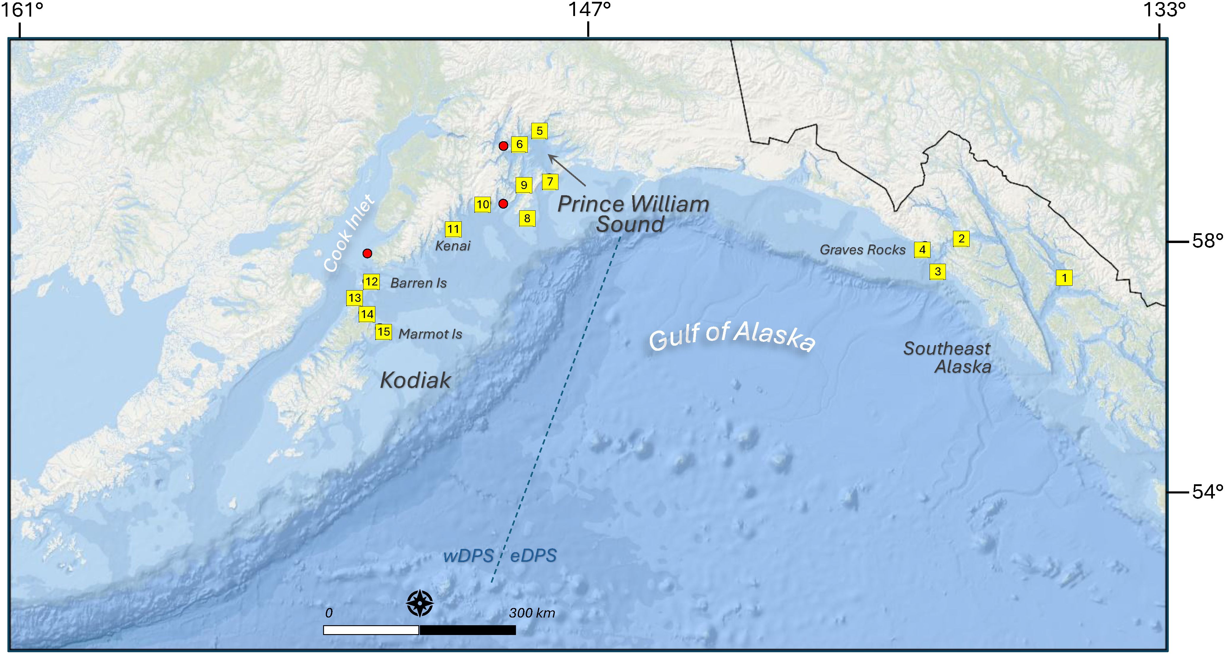
Figure 1. Map of Steller sea lion Eumetopias jubatus rookeries and sites where scat and/or water samples were collected in the Gulf of Alaska during summer and fall, 2022–2023. Yellow boxes are 15 water sampling locations = 1: Frederick Sound, 2: Icy Straits, 3: White Sisters rookery, 4: Graves Rock rookery, 5: Glacier Island, 6: Dutch Group, 7: Seal Rocks rookery, 8: Fish Island rookery, 9: the Needle, 10: Procession Rocks, 11: Rugged Island, 12: Barren Islands (Sugarloaf and Ushagat rookeries), 13: Latax Rocks, 14: Sea Otter Island, 15: Marmot Island rookery. Additional scat collection sites in red dots: Perry Island (near 6), Danger Island (near 10), and Flat Island (near 12). Scale = 150 km. Blue dotted line indicates the boundary between the western and eastern populations (wDPS/eDPS).
The historic SSL decline may have been caused by an abrupt reduction in carrying capacity linked to prey community restructuring following a rapid shift from cold to warm ocean regimes, in an area also important to large commercial fisheries (Anderson and Piatt, 1999; NMFS, 2008). The very large and extensive declines observed for SSL in this area suggested this species may be particularly vulnerable to rapid shifts in conditions and/or changes in the prey community. This was puzzling as SSL are generalist predators that feed on a variety of pelagic, benthic and demersal fishes with strong seasonal and regional patterns that likely reflect seasonal and regional variation in the availability of different prey (e.g., due to schooling, migration, and spawning behavior; Sinclair and Zeppelin, 2002). During the period of decline, their diverse diet included Alaska pollock and Atka Mackerel as the most common prey, with Pacific cod, salmon, forage fish (herring, sandlance, capelin), rockfish, skates and cephalopods also important (Sinclair and Zeppelin, 2002; Trites et al., 2007). Foraging behavior of adult female SSL also reflected that of a generalist predator able to exploit a variety of prey throughout the water column (Rehberg et al., 2009); adult male foraging behavior has not yet been studied. Adult females are shallow divers in general with most dives observed well within their aerobic dive limits (Merrick and Loughlin, 1997; Rehberg et al., 2009; Lander et al., 2020). Mixed foraging strategies have been observed (e.g., benthic foraging nearshore and deeper dives, such as for vertically migrating prey, when offshore), together with marked individual variation in foraging behaviors (Lander et al., 2020) and consistent individual movement patterns suggesting utilization of known prey patches (Rehberg et al., 2009). Although not observed in Washington (Lewis, 2022) and not yet well studied, diets may differ among sexes as males consumed more bottom fish than adult females at rookeries in summer in SEAK, perhaps due to reduced behavioral or physiological constraints for males (Trites and Calkins, 2008). Subsequent studies found that from 1999–2009 the areas of greatest population recovery were associated with greater diet diversity, increased forage fish consumption, and reduced reliance on pollock (McKenzie and Wynne, 2008; Sinclair et al., 2013). However, the diet of SSL in the Gulf of Alaska has not been monitored since 2009, and the areas of the western population east of Cook Inlet, which were most affected by recent marine heatwaves, have only rarely been studied (Pitcher, 1981; Maniscalco, 2023).
Additional potential health-related stressors linked to prey consumption for SSL include helminth infections and exposure to biotoxins (Moles and Heintz, 2007; Lefebvre et al., 2016). High infection rates of parasitic intestinal worms acquired through their fish and cephalopod prey are common in marine mammals (Dailey, 2001). Worm infections may lower fitness due to gastric ulcers or lesions, reduced nutritional intake, anemia, inflammation, bacterial infections and energy burden; in the worst cases, stomach or intestinal perforations may rarely result in peritonitis and death (reviewed by Mastick et al., 2024). While combined effects of multiple stressors on wildlife health are often complex (Grabner et al., 2023), high rates of infection may indicate populations with reduced immunity or compromised health due to other pathogens, poor nutrition or exposure to multiple, sublethal stressors (Dickinson et al, 2024). Few studies of helminth infections in SSL or their prey are available (Shults, 1986; Moles and Heintz, 2007), but in general, infection rates are not well studied in this species. Incidence of marine-mammal infecting helminths in SSL prey was higher in declining versus increasing populations, suggesting an additional population stressor (Moles and Heintz, 2007). Additionally, a 283-fold increase in infections by Anisakis spp. roundworms has been observed worldwide over the last four decades (Fiorenza et al., 2020), with similar increases observed specifically in marine mammal prey, indicating risk of Anisakis spp. infections is increasing for marine mammals globally (Mastick et al., 2024). A measure of current helminth exposure in SSL would benefit population monitoring by providing an assessment of this potential population stressor.
The neurotoxin saxitoxin (STX) produced by blooms of the dinoflagellate Alexandrium, is prevalent and widespread at low concentrations throughout the food web in the eastern Gulf of Alaska (Vandersea et al., 2018; Van Hemert et al., 2020). SSL and other marine mammals are exposed to STX in Alaska through their prey (Lefebvre et al., 2016). STX and its derivatives cause the human illness known as paralytic shellfish poisoning which at lower concentrations cause muscle weakness, reduced coordination, and incoherence and at high concentrations, respiratory paralysis and death in humans and marine wildlife (Landsberg, 2002). Chronic exposure to STX has been linked to brain damage and diminished spatial memory in mammals (Sun et al., 2021) and to reduced immunity and antioxidant defense in fish (Haque et al., 2022). Effects of STX on marine mammals are not well studied, but STX was a suspected or known cause of several marine mammal mortality events (reviewed by Lefebvre et al., 2016). Harmful algal blooms are increasing in severity and frequency with ocean warming, especially in the nearshore environments which SSL inhabit (Gobler et al., 2017; Wells et al., 2020), and increased STX toxicity and prevalence is also expected due to ocean acidification (Roggatz et al., 2019). STX was detected at low concentrations in fecal samples of 4 individual SSL collected in the Gulf of Alaska from 2004–2013 (Lefebvre et al., 2016), but sample size was small (n = 42 tested) and recent data are lacking. A larger sample of SSL scats from Washington from 2011–2013 (n = 373), found higher prevalence (42% positive) of STX in samples at low concentrations year-round (Akmajian et al., 2017).
Diets of SSL have most often been studied through analysis of hard parts in scats or stomachs (Pitcher, 1981; Sinclair and Zeppelin, 2002), but also through analysis of prey DNA using polymerase chain reaction (PCR) techniques (Tollit et al., 2009; Maniscalco, 2023) and metabarcoding (Lewis, 2022). DNA metabarcoding is a high-throughput next-generation sequencing approach which can identify multiple species simultaneously in a single sample using DNA occurring in the environment (eDNA) or bulk DNA samples and DNA barcodes, short DNA sequences that identify species by matching them to a DNA reference library (Hebert et al., 2003; Taberlet et al., 2012). For diet studies, DNA metabarcoding of fecal samples provides the benefits of high taxonomic resolution, the detection of rare prey and the identification of prey from soft tissues, coupled with the cost and time efficiency of a mass-target system (Pompanon et al., 2012; Ando et al., 2020). DNA metabarcoding of eDNA in seawater also provides a cost-effective, powerful method for surveying ecosystem components and prey resources in the marine environment available to apex predators (Thomsen et al., 2016; Visser et al., 2021; Boyse et al., 2024). How prey availability and composition influence population resiliency of SSL has been a central question since the severe population decline began over four decades ago (Merrick et al., 1997) but it remains largely unanswered due especially to the difficulty and cost in monitoring the nearshore prey field utilized by SSL by traditional survey methods (Womble and Sigler, 2006; Adams et al., 2008; Winter et al., 2009; Rand et al., 2019).
In this study we used DNA metabarcoding of SSL scat samples collected from Prince William Sound (PWS) to Kodiak Island, and seawater samples collected near SSL aggregations, to examine broad-scale geographic variation in SSL diet composition and prey resources in the Gulf of Alaska in 2022–2023. We used multivariate statistics to examine variation in diet composition, helminth exposure and STX exposure among regions, seasons (July vs. October) and sexes, and to assess diet items most associated with these potential stressors. Finally, we present data for comparing regional diet composition in scats versus seawater, and for comparing regional STX concentrations versus abundance of STX-producing microorganisms (Alexandrium spp. dinoflagellates) in seawater to assess the feasibility of monitoring this suite of related factors and their influence on SSL population dynamics by these methods.
2 Methods
2.1 Sample collection and preparation
2.1.1 SSL scat samples
Both in the field and laboratory, a rigorous quality control protocol was followed to prevent contamination of samples from exogenous DNA (King et al., 2008; USFWS, 2022). In July and October 2022 and 2023, 251 scats were collected at 8 sites in 3 regions in the Gulf of Alaska: Cook Inlet, Kodiak Island, and PWS (Figure 1; Table 1). Entire fresh scats (regardless of size or characteristics) were collected using clean, disposable gloves and spoon for each sample, placed in Ziploc® bags and stored at -20 °C within 6 hours of collection (Thomas et al., 2022).
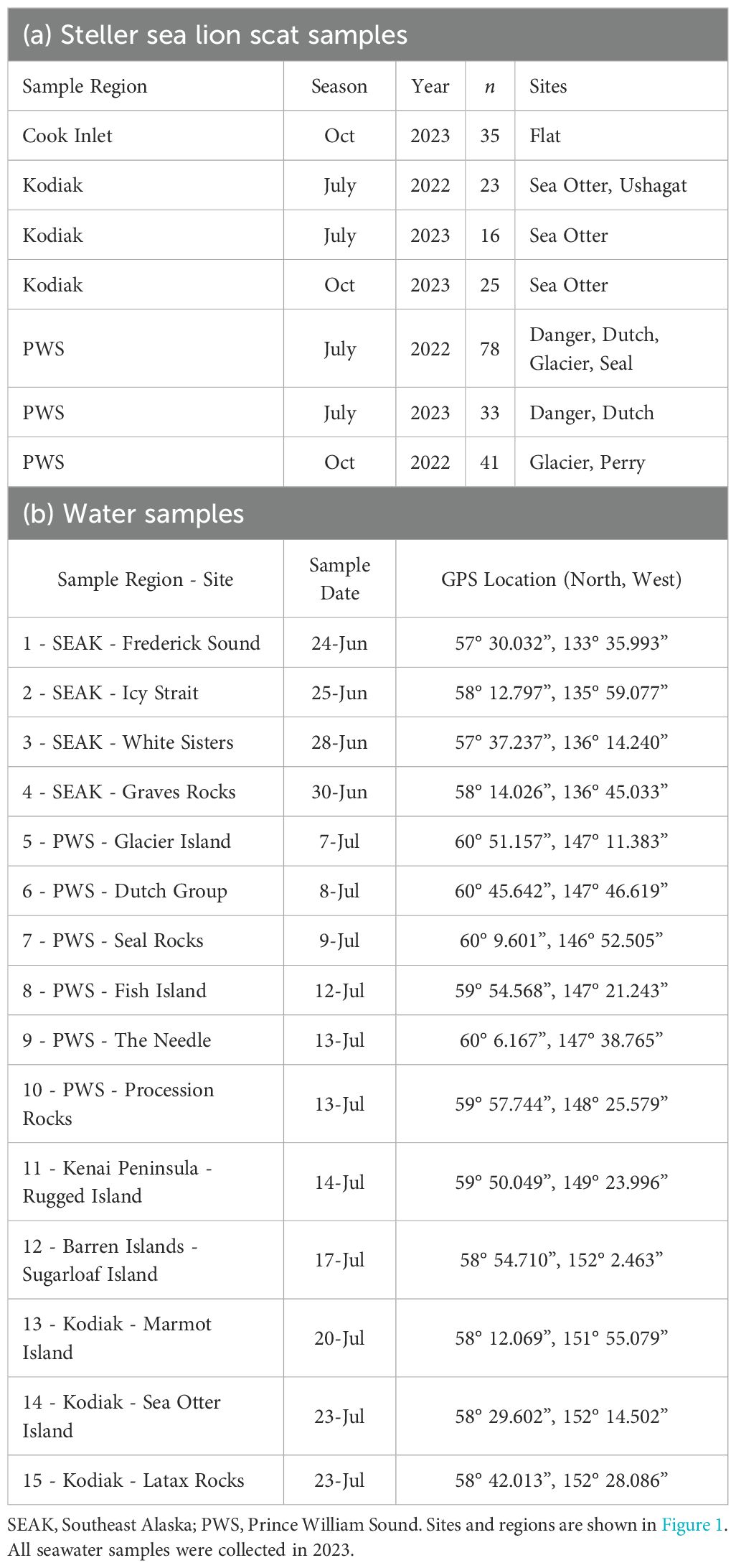
Table 1. (a) Steller sea lion Eumetopias jubatus scat samples and (b) 10m depth seawater samples collected from 2022–2023 in the Gulf of Alaska by season, year, region and site to assess nearshore prey resources and diet composition using DNA metabarcoding.
Sample preparation followed protocols detailed for harbor seal diet metabarcoding studies (Thomas, 2015; Thomas et al., 2022). To prepare samples for laboratory analysis, each frozen sample was partially thawed on a sterilized workspace and a ~4mL subsample was transferred to a 5mL cryovial using sterilize instruments and immediately stored at -80°C for STX analysis. The remaining sample was submerged in 95% molecular-grade ethanol in 500mL or 1L Histoplex® jars lined with 1gal-sized paint strainers made of 200μm nylon mesh and then, after fully thawed, manually homogenized with a clean wooden tongue depressor by gentle stirring for ~3–5min per sample. The paint strainer with hard-part and non-scat items (e.g., rocks or debris if present) was removed from the jar, placed in a Ziploc® bag, and archived at -20°C for future hard-part analysis. The scat matrix ethanol mixture was stored at -20°C for 24 hours to allow the matrix to settle out of solution. A clean, disposable pipette was used to transfer two subsamples of the matrix: 0.5mL to a 2mL cryovial (for DNA extraction) and 1mL to a 5mL cryovial (for archiving), which were topped off with 1.5mL and 3mL of fresh 95% molecular-grade ethanol (e.g., 1:3 ratio of matrix to ethanol), respectively, and stored at -80°C. This procedure was used to ensure sample homogenization to maximize detection of diet items and reduce sample variance, as food items are not distributed equally within scat samples (Deagle et al., 2005).
2.1.2 Seawater samples to assess SSL prey field
From 24 June–23 July 2023, seawater samples were collected via a 1.7L Niskin bottle (Model 1010, General Oceanics, Inc., Miami, FL, USA) at a depth of 10m during Gulf-wide SSL population surveys. Our goal for this sampling was to acquire initial data as a pilot study to determine if a fast, efficient seawater sampling protocol would provide useful data on nearshore fish assemblages as an efficient addition to our regular, annual SSL surveys. A standard depth of 10m was chosen for the following reasons: (1) Dives of adult female SSL from the western population were relatively shallow with median or average dive depths of 21–28m during summer and winter (Merrick and Loughlin, 1997; Lander et al., 2020); up to 54% of dives of adult females were between 4–10m and >90% were <50m (Merrick and Loughlin, 1997). (2) This depth allowed us to sample below the water’s surface but was shallow enough to allow quick, hand-deployment of the Niskin bottle; hand deploying to deeper depths, especially in strong currents, could be prohibitive. (3) We desired information on the nearshore environment and did not assume foraging areas or foraging depths of SSL; a rigorous, comprehensive study evaluating the utility of eDNA to study vertebrate diversity found equivalent information across 10–80m sampling depths suggesting vertical mixing may provide information on fish diversity from throughout the upper water column, even from surface water collections (Closek et al., 2019).
Three 1.7L replicates per site were collected at 15 sites, at least 0.5km distant from SSL aggregations, from SEAK to Kodiak Island (Figure 1). Seawater was filtered directly from the Niskin bottle in the field using a Smith-Root eDNA Citizen Scientist Sampler and 5µm self-preserving polyethersulfone filters (Smith-Root, Inc., Vancouver, WA, USA). Five negative controls of distilled water were processed in triplicate at weekly intervals throughout the sampling period to test for contamination of the field sampling system. Filters were stored in a cool, dry, and dark location until subsequent DNA extraction within 3 months post sample collection.
2.2 DNA metabarcoding
2.2.1 DNA extraction
All laboratory work for scat and seawater samples was performed at the Washington Department of Fish and Wildlife’s Molecular Genetics Laboratory (WDFW-MGL) in AirClean 600 Workstations equipped with HEPA filtered air and UV light irradiation. Work surfaces and equipment were sterilized with 10% bleach and exposed to UV-C light for one hour to neutralize exogenous DNA. Seawater filter DNA was extracted using DNeasy™ Blood & Tissue Kits (Qiagen, Hilden, Germany) following the methods of Pilliod et al. (2013) with one extraction negative control processed per batch of 47 filters. SSL scat DNA was extracted using QIAamp™ Fast DNA Stool Mini Kits (Qiagen) following a customized protocol for pinniped scat (Deagle et al., 2005) with one extraction negative control processed per batch of 23 scats.
Library preparation - We assessed prey diversity using two genes, mitochondrial cytochrome c oxidase subunit I (COI) and 12S rRNA MiFish (12S) genes, to provide better biodiversity coverage. The 12S rRNA MiFish-U primer was optimal for bony fishes (Actinopterygii) and informative of cartilaginous fishes (Chondrichthyes; Miya et al., 2015), whereas the COI primer amplifies all metazoans, including cephalopods (Arfin et al., 2023) which are potentially important SSL prey (Pitcher, 1981). For pinniped scat diet studies, the COI gene (although a different fragment than used in our study) has been used in particular to distinguish salmon species (Lewis, 2022; Thomas et al., 2022; Trzcinski et al., 2024). The COI and 12S genes were amplified in separate reactions. The COI gene region was amplified with the Leray-XT primers (Wangensteen et al., 2018) and the 12S gene region was amplified with the MiFish-U primers (Miya et al., 2015). The Leray-XT primers amplified a 313bp gene fragment and included the forward primer mlCOIintF-XT 5′-GGWACWRGWTGRACWITITAYCCYCC-3′ (Wangensteen et al., 2018), modified from the original mlCOIintF primer developed by Leray et al. (2013), and the reverse primer jgHCO2198 5′-TAIACYTCIGGRTGICCRAARAAYCA-3′ (Geller et al., 2013). The MiFish-U primers amplified a 170bp gene fragment and included the forward primer 5′-GTCGGTAAAACTCGTGCCAGC-3′ and the reverse primer 5′-CATAGTGGGGTATCTAATCCCAGTTTG-3′ (Miya et al., 2015).
PCRs were performed in 30μL volumes using the Multiplex PCR Kit (Qiagen). COI reactions contained 15μL (1X) of multiplex master mix, 0.8μM of each primer and 2μL of template DNA with thermal cycling conditions as follows: 95°C for 10min, 35 cycles of 95°C for 60s, 50°C for 60s, and 72°C for 60s, and a final extension of 72°C for 5min. 12S reactions contained 15μL (1X) of multiplex master mix, 2μM of each primer and 1μL of template DNA with thermal cycling conditions as follows: 95°C for 10min, 14 touchdown cycles of 94°C for 30s, 69.5-50°C for 30s, and 72°C for 90s, 25 cycles of 94°C for 30s, 50°C for 30s, and 72°C for 45s, and a final extension of 72°C for 10min. A PCR negative and positive control were included on each 96-well PCR plate. The negative control consisted of sterile molecular grade water in lieu of template DNA and kangaroo DNA was used as a positive amplification control.
PCR products were size selected using Mag-Bind® TotalPure NGS (Omega Bio-tek, Inc., Norcross, GA, USA) beads. A ratio of beads to product of 0.8X was used for the COI amplicon and 1.2X was used for the 12S amplicon. Sample amplicons were then indexed with Nextera DNA unique dual (UD) indexes (IDT® for Illumina®), normalized using the SequalPrep™ Normalization Plate Kit (Invitrogen) and each 96-well plate was subsequently pooled. Plate libraries were bead cleaned at a 0.8X bead ratio, quantified with a Qubit® fluorometer (Life Technologies), and pooled by amplicon. Amplicon libraries were quantified and normalized to 4nM prior to loading at a 1:1 12S to COI ratio on the NextSeq™ 1000 platform with 25% PhiX Control v3 Library (Illumina, Inc., San Diego, CA, USA). Seawater filters were sequenced using the NextSeq™ 1000 P1 (300 cycles) Reagent Kit for single end reads and scats were sequenced using the NextSeq™ 1000 P1 (600 cycles) Reagent Kit for paired end reads (Illumina, Inc.).
2.2.2 Bioinformatics
Amplicon sequence data were analyzed separately (COI and 12S) using either stand-alone QIIME 2 (Bolyen et al., 2019) and DADA2 (Callahan et al., 2016) or with Tourmaline (https://github.com/aomlomics/tourmaline), a Snakemake pipeline that wraps QIIME 2 and DADA2, providing reproducible metabarcoding analysis. Adapters and primers were trimmed from demultiplexed FASTQ reads using Cutadapt (Martin, 2011). The program DADA2 was used to quality filter reads. Reads were truncated to a common length (210bp for the COI amplicon and 160bp for the 12S amplicon) with a maximum number of expected errors=2, chimeras were removed (consensus method), and amplicon sequence variants (ASVs) were exported.
To assign COI taxonomy, a custom reference database was generated that included existing sequence data for Alaska SSL prey and fishes and cephalopods observed in the Resource Assessment and Conservation Engineering (RACE) Gulf of Alaska summer biennial bottom trawl surveys (https://www.fisheries.noaa.gov/foss/f?p=215%3A28) from 2015–2023, the MIDORI database (Machida et al., 2017), and all mitochondrial COI sequences in the National Center for Biotechnology Information (NCBI) nucleotide database. To assign 12S taxonomy an rCRUX (Curd et al., 2024) generated reference database was used that included all 12S sequences in the NCBI nucleotide database, an additional custom database comprised of all Actinopterygii (bony fishes) mitogenomes (Gold et al., 2023), and sequences available for published SSL prey and for fishes and cephalopods in the RACE surveys. If voucher specimen sequence data were publicly available, they were included in the reference library. If sequences were identical, assignments were produced at a higher taxonomic resolution.
Global taxonomic alignments between query and reference sequences were performed using the VSEARCH consensus taxonomy classifier (Rognes et al., 2016) and matches with ≥ 97% identity were retained. Read counts for each operational taxonomic unit (OTU) per sample were tallied.
2.3 Sex identification using SSL scat samples
DNA extract from 250 scat samples was provided to the Alaska Department of Fish and Game’s Gene Conservation Laboratory to determine SSL sex identification by adapting existing protocols (Lewis, 2022; Gard et al., 2024). Briefly, sex-specific oligonucleotides developed for SSL were used to assess the presence of X- and Y-chromosomally linked genes (ZFX and SRY) in the scat DNA. DNA was amplified on a GeneAmp™ PCR System 9700 with a Multiplex PCR Kit (Qiagen), 0.2μM of each primer, and 4μL of DNA using Gene Conservation Laboratory’s standard 14 cycle preamplification PCR protocol with thermal cycling conditions as follows: 95°C for 15min, 14 cycles of 95°C for 15s and 60°C for 4min. The individual primers and probes from the two qPCR assays were then combined into a single 80X sex ID genotyping assay (16μM each probe, 72μM each primer). Final concentrations of the probes and primers in the PCR reaction were 0.2µM and 0.9µM. Genotypes were collected on an Applied Biosystems™ QuantStudio 12K Flex using their 2X TaqMan™ GTXpress™ Master Mix, 1X genotyping assay, and 2.5μL of 0.1X preamplification PCR product according to the PCR protocol of Schwarz et al. (2018). Genotypes were scored at 42 cycles.
2.4 Saxitoxin in SSL scat samples
In addition to scat samples from the current study, 8 samples from the Kenai Peninsula collected by the Alaska SeaLife Center (Jan–May 2017–2019) and 12 samples from SEAK (July 2016) were included. STX in scat samples was measured by the Northwest Fisheries Science Center’s Wildlife Algal-Toxin Research and Response Network (WARRN-West) laboratory, following the protocol of Lefebvre et al. (2022). Briefly, the ~4mL raw scat samples provided to the lab were thawed slowly in a small cooler, stirred thoroughly, and ~1mL per sample was aliquoted into 14mL polypropylene screw-cap tubes (Falcon-BD). For STX extraction, 50% methanol was added to samples in a 1:4 wt/v ratio (1 part sample, 3 parts solvent) and samples were vortexed. Samples were homogenized for 60s using an Omni GLH 850 homogenizer and the homogenized sample was then centrifuged at 3,082xg (Jouan CR3i centrifuge) for 20min at 4°C. The supernatant was added to a 0.22μm Durapore™ membrane filter (Millipore Ultrafree-MC centrifugal concentration device) and filtered in a desk-top microcentrifuge (AccuSpin Micro 17, Fisher Scientific) for 3min at 12,000rpm. Sample extracts were stored at 4°C until analysis by enzyme-linked immunosorbent assay (ELISA).
STX in samples was quantified using a commercially-available Abraxis saxitoxin ELISA kit (PN 52255B: Gold Standard Diagnostics, Horsham, PA). Standards solutions provided in these kits were loaded along with the samples on plates and a standard curve was derived for each plate. Manufacturer instructions were followed with modifications for matrix effects for marine mammal feces determined by Hendrix et al. (2021) with sample dilution of 1:50 filtered sample extract:sample diluent solution provided with the ELISA kit. The ELISA kit was designed to measure STX with some limited cross-reactivity to several other paralytic shellfish poison (PSP) toxins. Consequently, all PSP concentrations are listed as STX equivalents and may underestimate the presence of other congeners.
2.5 Statistics
2.5.1 Diet and prey data summaries
We included taxa for bony and cartilaginous fishes for the 12S data and for these fishes, cephalopods, and other potentially interesting taxa (e.g., parasitic worms) for the COI data. For both metabarcoding datasets for scat samples, we performed the following minimum sequence threshold filtering steps prior to statistical analyses: (1) samples with <20 total prey assigned reads were removed (Trzcinski et al., 2024), (2) OTUs were assigned into prey groups at the species level or at the genus level for groups in which significant assigned reads were only to genus level (Deagle et al., 2019), (3) global (summed across all samples) total assigned reads per prey group were calculated and groups with <100 total assigned reads were removed, and (4) prey groups <0.01% of the per sample proportion of total prey assigned reads were removed to normalize detection rates among samples which may vary in read depth (Pornon et al., 2016; Richardson et al., 2019) to assess region*season variation in diet. For seawater samples, all assigned fish reads were used without filtering data, and assigned reads for the three replicates per site were summed to provide sufficient sample size.
Following the methods of Deagle et al. (2019), region*season diet composition was calculated using both weighted percent frequency of occurrence (wPOO; i.e. split-sample frequency of occurrence; Tollit et al., 2017; Equation 1) and relative read abundance (RRA; Equation 2):
where T is the number of diet items (taxa), S is the number of samples, and I is an indicator variable such that I i,k= 1 if diet item i was present in sample k, 0 if not. We used RRA to summarize diet composition (Thomas et al., 2022; Trzcinski et al., 2024) but also used wPOO for a thorough presentation of the data (Deagle et al., 2019). RRA may most accurately reflect diet composition consumed at the population level, especially when many and similar diet items occur among samples but can be biased by differences in barcode recovery rates due to biological and technical factors (e.g., variability in number of mitochondria in tissue among different prey, preferential primer binding, bioinformatics methods; Deagle et al., 2019; Thomas et al., 2022). wPOO is less affected by recovery biases but may overestimate the consumption of less frequently occurring diet items, and include more secondary diet items (Deagle et al., 2019; Thomas et al., 2022). wPOO was assessed to allow for the inclusion of potentially rare diet items.
2.5.2 Cluster analysis: diet items occurring together in scats
A presence-absence matrix of diet items based on individual scats was created for each gene separately. Diet items with <10 total occurrences were pooled into similar groups. We then calculated dissimilarity scores as 1 - the Jaccard Index for each pair of diet items, where the index was calculated as n scats with both diet items occurring/n scats with either diet item occurring (Jaccard, 1912). The resulting distance matrix was input for the hclust function (stats package in R 4.1.3, R Core Development Team, 2022) to perform hierarchical clustering analysis using the “complete” method.
2.5.3 Diet multivariate analysis
Principal component analysis was used to visualize important characteristics of diet composition using function prcomp (Bakker, 2024). To assess differences in diet composition by group (region*season and sex) and continuous covariates (STX concentration and parasite load), we performed permutational multivariate analysis of variance using distance matrices (PERMANOVA; Anderson, 2001; McArdle and Anderson, 2001). Bray-Curtis similarities were first calculated from the square root transformed matrix of RRA for diet items (RRA was a normalized and scaled index for a total of 100 reads per sample) using function vegdist in R package vegan (R Core Development Team, 2022; Oksanen et al., 2025). Function betadisper was then used to evaluate heterogeneity of variances among groups, and to visualize groups differences in means and dispersion via principal components (Anderson, 2006; Bakker, 2024). Finally, the variance in diet composition explained by group and continuous covariates was assessed via pseudo-F statistics using PERMANOVA and function adonis2 (Anderson, 2001). Pairwise comparisons of important group covariates were assessed using a Bonferroni correction for multiple tests (function pairwise.adonis2; Bakker, 2024).
2.5.4 Spatiotemporal diet diversity
Using RRA, we calculated the diet diversity per sample using species richness (the average number of diet items per sample separately for region*season groups) and the diet diversity across groups using Shannon Diversity Index (H’) calculated as: , where T is the number of diet items (taxa) observed for a region*season group, p is the proportion of the diet attributed to diet item i, and ln is the natural logarithm.
2.5.5 Presence/absence data, linear models, correlations and parasite level index
Chi-square tests were used to assess differences in presence/absence of parasites and STX among region*season groups. An index of parasite infection level was deemed useful for monitoring. For such an index, we accounted for sample quality differences by using the ratio of parasitic worm (tapeworms and parasitic nematodes) reads to SSL reads, by assuming these tissues are equally affected by sample quality and by the composition of other tissues in the sample. Linear models or non-parametric tests were used to assess differences in STX concentrations or the parasite level index. Pearson correlations were used to further explore relationships between diet item RRA and parasite RRA or STX concentrations.
3 Results
3.1 Scat: metabarcoding performance
For the 12S gene, 6 of 250 scat samples did not pass quality filtering parameters. The remaining samples, including controls, produced a total of 56.3M sequencing reads, of which 2.6M reads were unassigned. Excluding controls, the mean number of reads per sample (n = 244) was 228,936 and the mean number of reads per assigned OTU (n = 80) was 665,146. An additional 4 samples had no assigned reads, and 7 samples had no fish reads, and one sample had <20 fish reads, all of which were removed from further analysis (n = 232). For the remaining 232 samples (Table 2), the total fish reads per sample ranged from 102–561,237 (median=104,084) and 97% of samples had > 10,000 total fish reads.
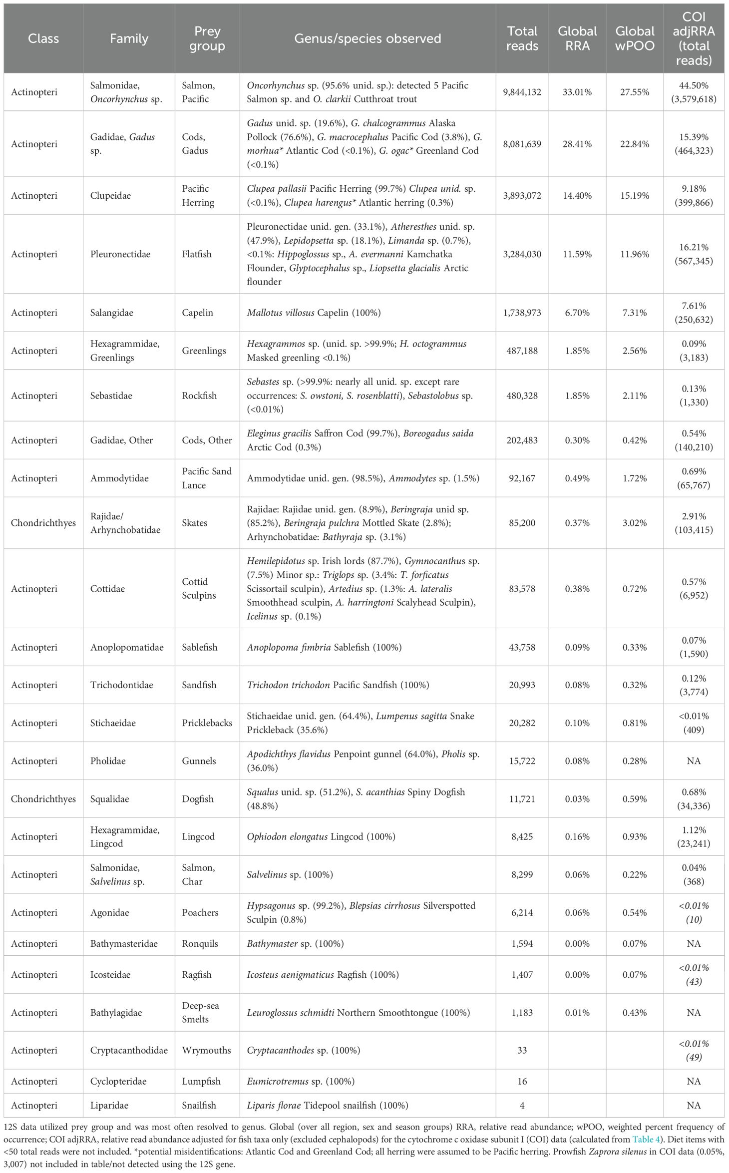
Table 2. 12S MiFish results: Global fish diet composition of Steller sea lion scats in summer and fall in the Gulf of Alaska, 2022–2023.
For the COI gene, 7 of 250 scat samples did not pass quality filtering parameters. The remaining samples, including controls, produced a total of 63.7M sequencing reads, of which 6M reads were unassigned. Excluding controls, the mean number of reads per sample (n = 243) was 258,065, the mean number of reads per assigned OTU (n = 193) was 293,705, and eukaryotes spanning 24 phyla were detected (Table 3). An additional 21 samples had no fish/cephalopod reads and five additional samples had <20 fish/cephalopod reads, all of which were removed from further analysis. For the remaining 217 samples (Table 4), the total fish/cephalopod reads per sample ranged from 21–487,517 (median=14,252) and 56.2% and 84.8% of samples had > 10,000 and > 1,000 total fish/cephalopod reads, respectively. Contamination of human DNA in samples and between controls and samples was negligible for both genes (< 0.0001% of total assigned reads).
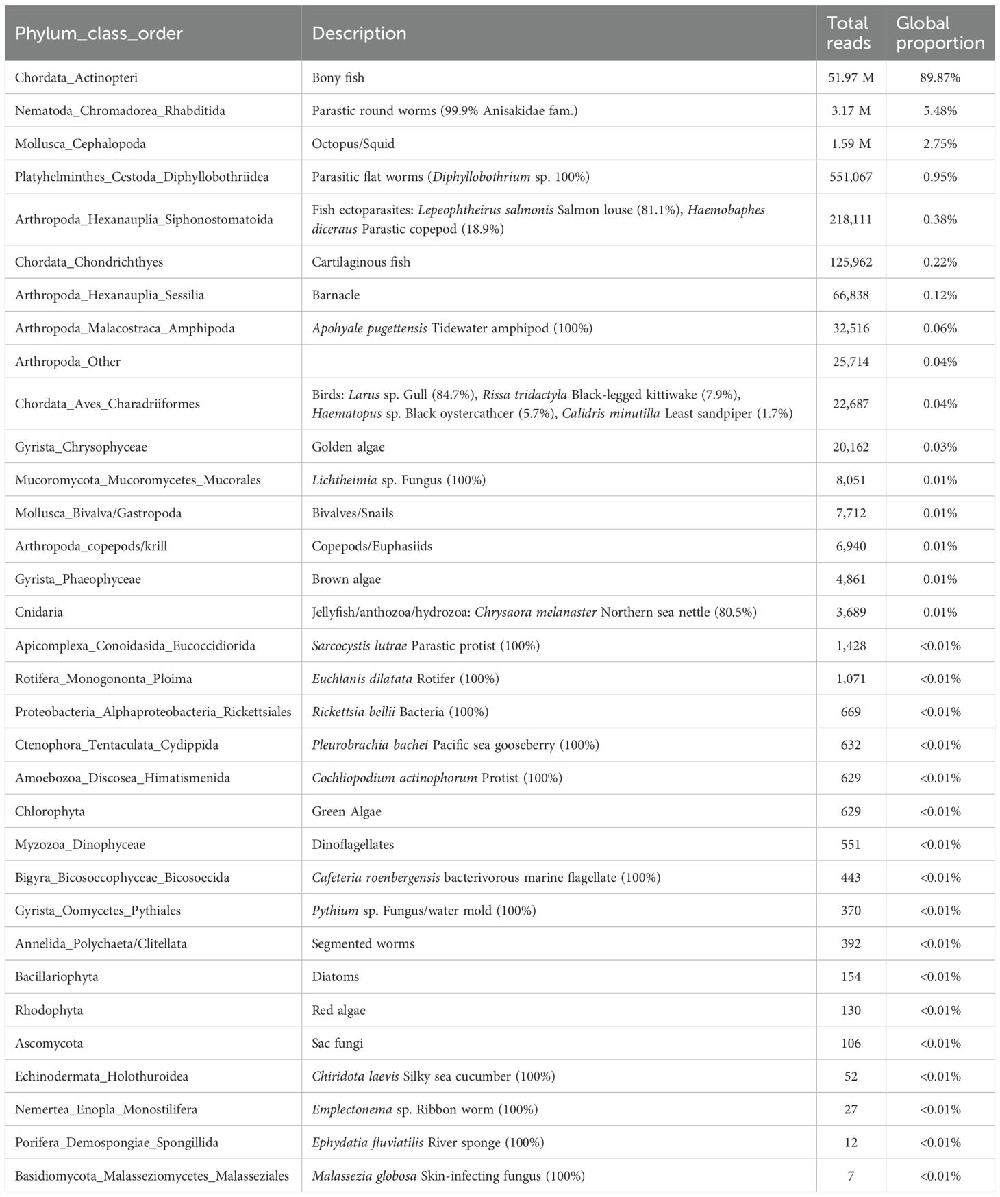
Table 3. COI results: Global proportion and total reads per taxa for all taxa (including non-prey but excluding mammals) detected in Steller sea lion scat collected in summer and fall in the Gulf of Alaska, 2022–2023, using data from the cytochrome c oxidase subunit I (COI) gene.
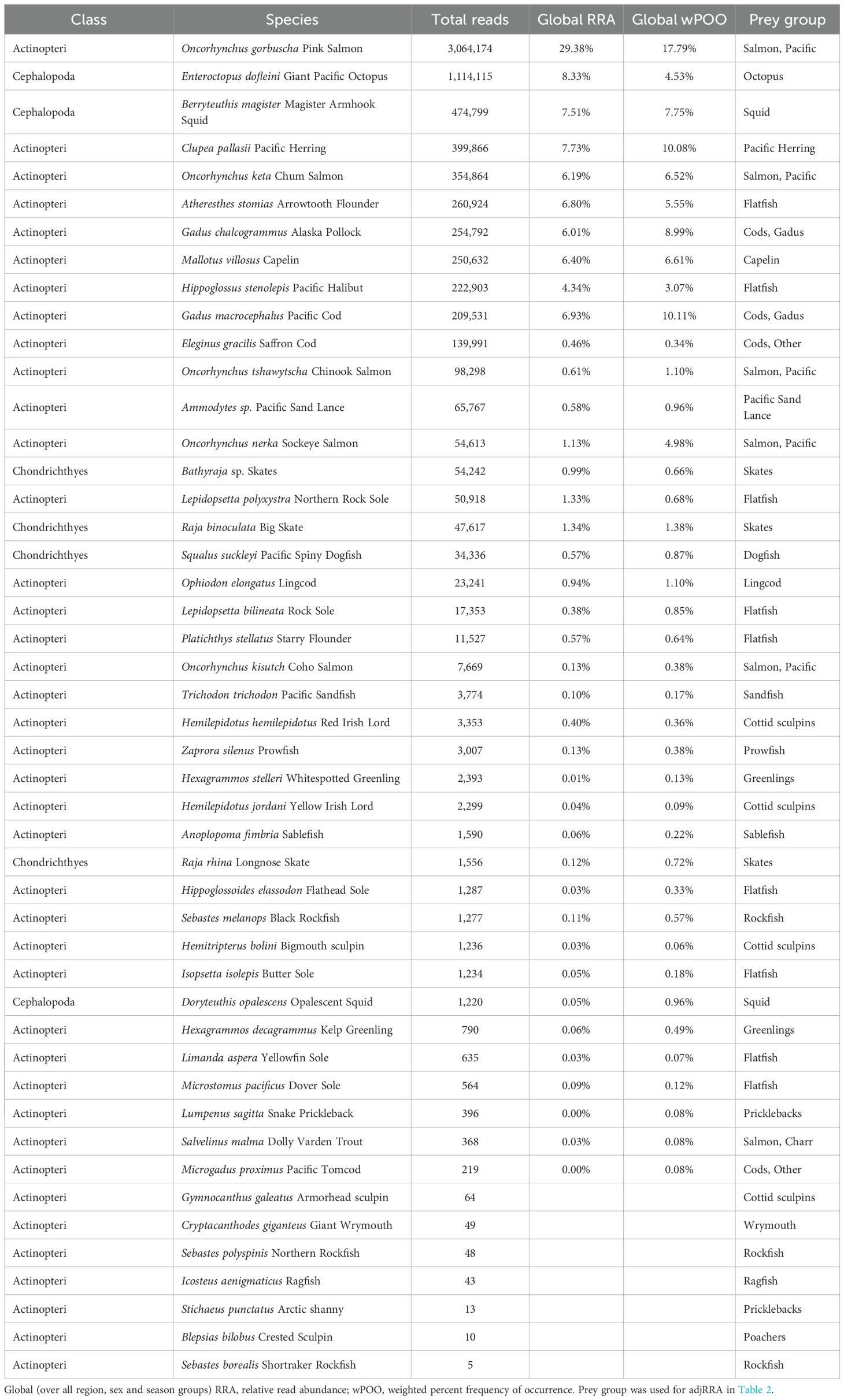
Table 4. COI results: Global fish and cephalopod diet composition of Steller sea lion scats in summer and fall in the Gulf of Alaska, 2022–2023 using data for the cytochrome c oxidase subunit I (COI) gene.
3.2 Scat: diet composition
3.2.1 Global patterns
For the 12S gene, 45.3% of total fish reads were assigned to species level, 50.5% to genus level, and 4.3% to family level. Fishes from 23 families were detected, nearly all (>99.7%) were assigned to class Actinopteri, with the few remaining to class Chondrichthyes (including dogfish and skates; Table 2). We created 25 prey groups by family and/or family_genus based on taxonomic resolution of the data. This resolved some groups to species because only one species was identified per genus (ragfish, sandfish, lingcod, sablefish, capelin, and northern smoothtongue; Table 2) or with one species that could be assumed per genus with only one species occurring in the Gulf of Alaska (i.e., Pacific sand lance and Pacific herring). Over all regions, sexes and seasons, SSL diet was dominated by Pacific salmon and Gadus spp. cods (gadids; 28.4–33.0% RRA each), followed by herring and flatfishes (11.6–14.4%), with capelin also in the top five diet items (6.7%; Table 2). Three prey groups were removed from further analysis due to <100 total reads (lumpsuckers, wrymouths and snailfish, 22 prey groups included; Table 2).
For the COI gene, 89.9% of the total non-mammal reads were assigned to bony fishes and other groups of interest (9.8%) included endoparasitic worms, cephalopods, cartilaginous fishes, and fish ectoparasites (Table 3). The remaining 0.3% of reads were likely exogenous DNA from the collection substrate and secondary prey items (e.g., 60% of these reads were from barnacles and tidewater amphipods; Table 3). Nearly all (99.6%) fish/cephalopod reads were assigned to species level, and 0.4% to genus level (Table 4). Species could be assumed for 2 of the 3 taxa at genus level (Ammodytes sp. = Pacific sand lance, Enteroctopus sp. = Enteroctopus dofleini giant Pacific octopus, the only species of this genus occurring in the North Pacific). Genus Bathyraja (skates) remained the only genus-level prey group as 72.2% of reads were assigned to genus level (Table 4). Fishes/cephalopods from 22 families were detected; 76.1% of prey reads assigned to class Actinopteri, 22.0% to cephalopods, and 1.9% to class Chondrichthyes (Table 4).
The number of species detected in the COI data was 47; 7 of these had <100 reads and were removed from further analyses (Table 4). Pink salmon had the most reads (29.4% RRA), followed by giant Pacific octopus (8.3%), magister armhook squid (7.5%), herring (7.7%), and 6 species with 4–7% RRA (Pacific halibut, arrowtooth flounder, Alaska pollock, chum salmon, capelin and Pacific cod; Table 4). Including only fishes in the COI data, the same 5 top prey groups occurred but compared to the 12S data, Pacific salmon were proportionally higher, and gadids and herring were proportionally lower in the COI data (Table 2). This was not due to the slight difference in the samples included in the two datasets, as the pattern was nearly identical when only the 209 shared samples between the two genes were considered.
3.2.2 Cluster analysis: diet items occurring together in scats
The 12S cluster analysis showed two prey groups tended to occur in the same sample: (1) rockfish and greenlings/sculpins and (2) flatfishes and cods. A mixture of the most prevalent diet items often occurred in the same sample (cods, flatfishes, salmon, and herring; Figure 2A). COI results suggested the species that tended to occur in the same sample were: (1) pollock and magister armhook squid, also tending to occur less frequently with herring and opalescent squid; (2) chum and sockeye with pink salmon; (3) minor flatfishes and dogfish/skates; (4) chinook and coho salmon with halibut and less so capelin; (5) Pacific cod and arrowtooth flounder, also with great Pacific octopus and greenlings/sculpins (Figure 2B).
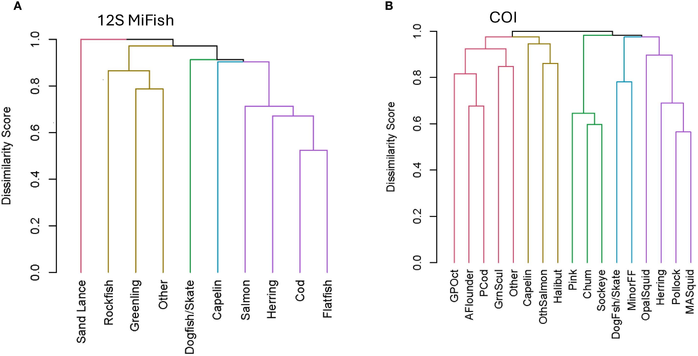
Figure 2. Steller sea lion prey groups or species occurring together in scats based on cluster analysis using presence/absence data based on the Jaccard Index; results for (A) the 12S MiFish gene (fish only) and (B) the cytochrome c oxidase subunit I gene (COI; fish and cephalopod). Plots were created with R package dendextend, choosing 5 color-coded clusters. GPOct, giant pacific octopus; AFlounder, Arrowtooth Flounder; GrnScul, Greenling/Sculpin pooled; OthSalmon, Other Salmon: chinook or coho; MinorFF, minor flatfish; OpalSquid, opalescent squid; MASquid, magister armhook squid; Other, pooled other category for rare taxa.
3.2.3 Spatiotemporal differences
In July, the most important diet items were Pacific salmon in PWS (less so gadids) and capelin in Kodiak (also gadids and flatfishes, Figures 3A, C and 4A, C). In October, herring was more prevalent in SSL diets in PWS and Kodiak but was not observed in Cook Inlet samples (Figures 3A, C and 4A, C). Gadids and flatfishes occurred at similar proportions across most regions and seasons but dominated fall scat samples from Cook Inlet (Figures 3 and 4). These patterns were similar based on both RRA and wPOO but, as expected (Deagle et al., 2019; Thomas et al., 2022), wPOO emphasized rare diet items (Figures 3 and 4).
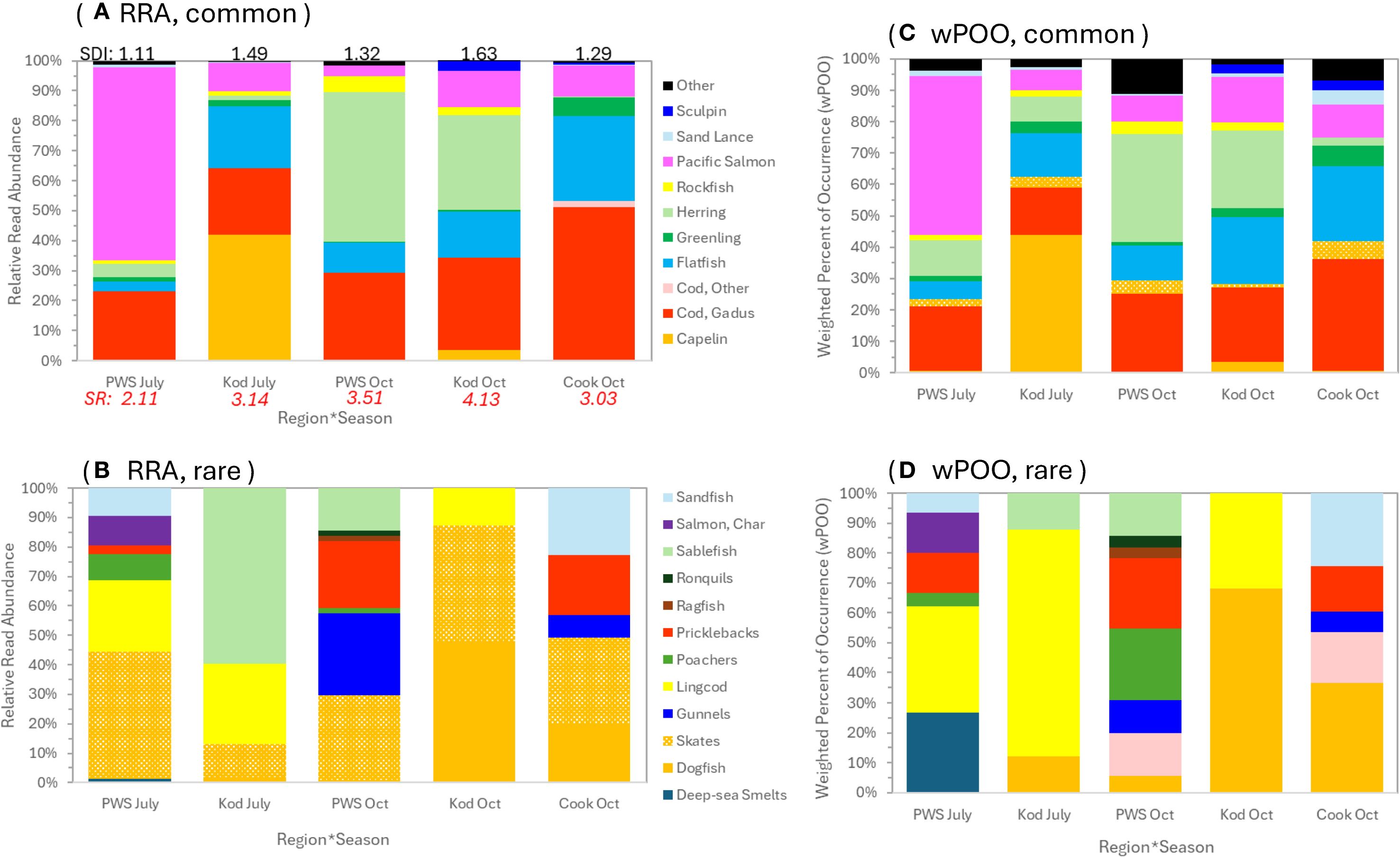
Figure 3. 12S MiFish prey composition of Steller sea lion scats from 2022–2023 in the Gulf of Alaska. (A, B) are relative read abundance and (C, D) are weighted percent of occurrence. Proportions shown are for prey that were dominant (A, C) and rare (B, D). (A, C) are true proportions and (B, D) are proportions of the “Other” category in (A, C) rescaled to 100%. In (A) is the Shannon Diversity Index (SDI) for the region*season group, and Species Richness (SR), the average number of taxa per sample for the group. Region*seasons were Prince William Sound (PWS), Kodiak (Kod) and Cook Inlet (Cook) in July or October.
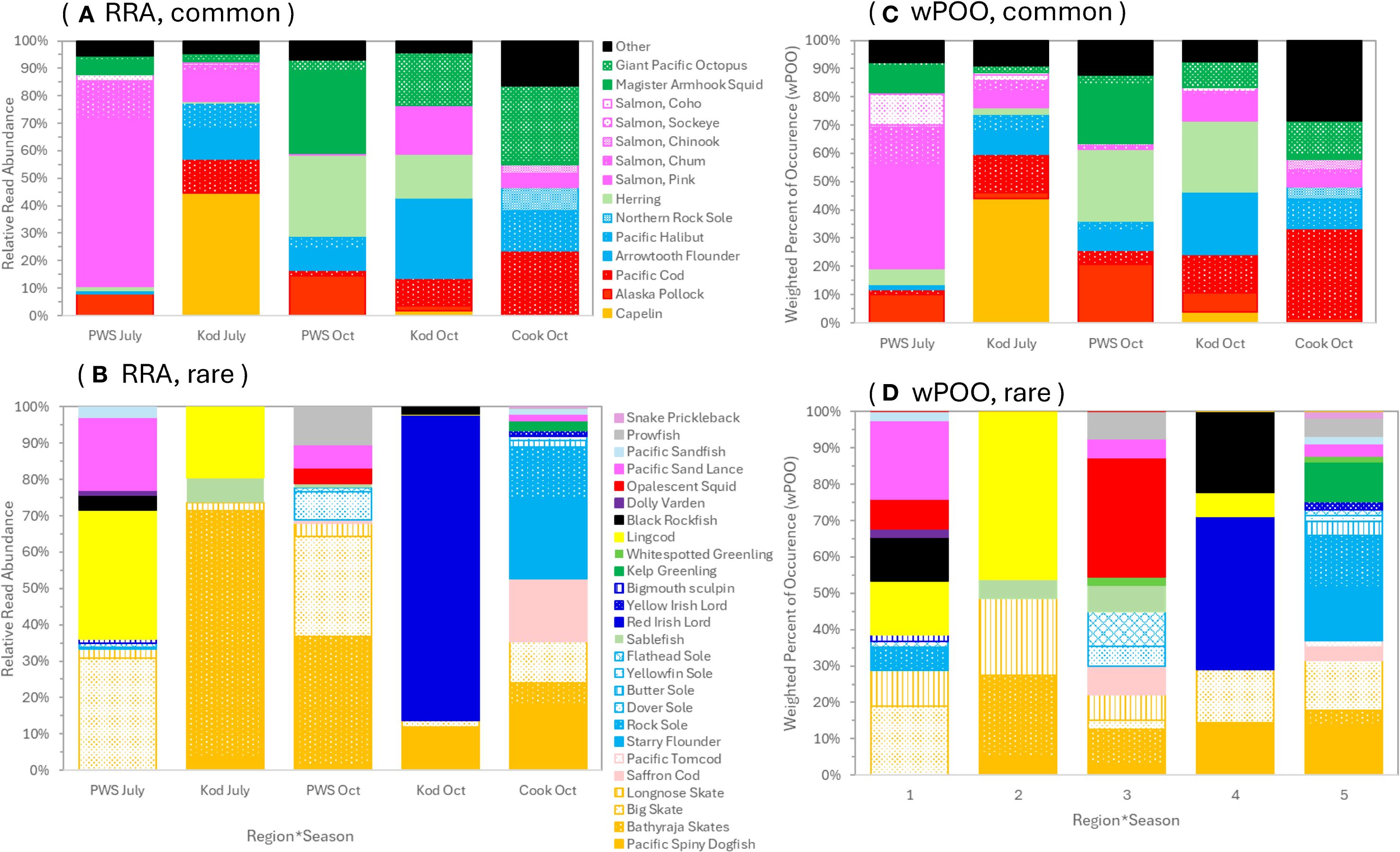
Figure 4. COI (cytochrome c oxidase subunit I) prey composition of Steller sea lion scats from 2022–2023 in the Gulf of Alaska. (A, B) are relative read abundance and (C, D) are weighted percent of occurrence. Proportions shown are for prey that were dominant (A, C) and rare (B, D). (A, C) are true proportions and (B, D) are proportions of the "Other" category in (A, C) rescaled to 100%. Region*seasons were Prince William Sound (PWS), Kodiak (Kod) and Cook Inlet (Cook) in July or October.
Spatiotemporal variation in the COI data was consistent with 12S results. However, diet proportions were altered by greater proportion of salmon reads in the COI data and also inclusion of two cephalopods consumed in relatively high numbers (a third cephalopod, opalescent squid, was also consumed but in low numbers, Figure 4). The COI data also distinguished species consumed for dominant diet items: for gadids, pollock was consumed in PWS versus Pacific cod in Kodiak and Cook Inlet (Figure 4). The majority of salmon consumed were pink salmon, especially in July in PWS; chum (in PWS in July) and chinook (in Cook Inlet in October) were less frequently consumed (Figure 4). Most flatfishes consumed were arrowtooth flounder, Pacific halibut and northern rock sole (Figure 4). Pacific sand lance (an important SSL prey in Kodiak from 1999–2005; McKenzie and Wynne, 2008) was rarely detected, however one sample contained 100% sand lance based on 12S data (Figures 3 and 4). Cottid sculpins detected in Kodiak in October in the 12S data were likely red Irish lord, as indicted in the COI data (Figures 3 and 4). Rockfishes were rarely detected, and black rockfish was the only species detected (Figures 3 and 4).
Most samples contained several diet items. Based on 12S RRA results, the average number of diet items per sample based on species richness ranged from 2.11 – 4.13 among regions and seasons (Figure 3A). An average of 61.3% over region*season groups had 3 or more diet items per sample (range: 29.4 – 91.7%); and 17.6% had only 1 diet item per sample (range: 0.0 – 39.2%). The same diet items also occurred across many samples: 0.00– 0.02% of samples did not contain at least 1 of the top 4 diet items per region*season group, and an average of 75.7% of samples (range: 51.0 – 100%) had 2 or more of the top four diet items for those groups. Similar to species richness per sample, the Shannon Diversity Index suggested higher diet diversity (based on our broad prey groups) in fall (1.32 and 1.63) than summer (1.11 and 1.49), and in Kodiak (1.49 and 1.63) than PWS (1.11 and 1.32; Figure 3A).
After pooling diet items with number of samples < 20 into prey group “other” for the 12S RRA results (resulting in 9 prey groups), four principal components accounted for 93.0% of the variation (cumulative proportions to PCA 1–3 were 44.1%, 66.1%, 80.8%, respectively); differences between the top components were due especially to gadids and salmon, and less so herring, then flatfishes and capelin (Figure 5A). PERMANOVA supported group differences (p = 0.001) and pairwise comparisons indicated all groups differed (all p = 0.01) except for PWS in October and Kodiak in October (p = 0.38). Centroids were especially different from Cook Inlet in October and PWS in July for top components (Figure 5B). Dispersion was sufficiently similar among groups (p = 0.09) supporting different group centroids (Figure 5B).
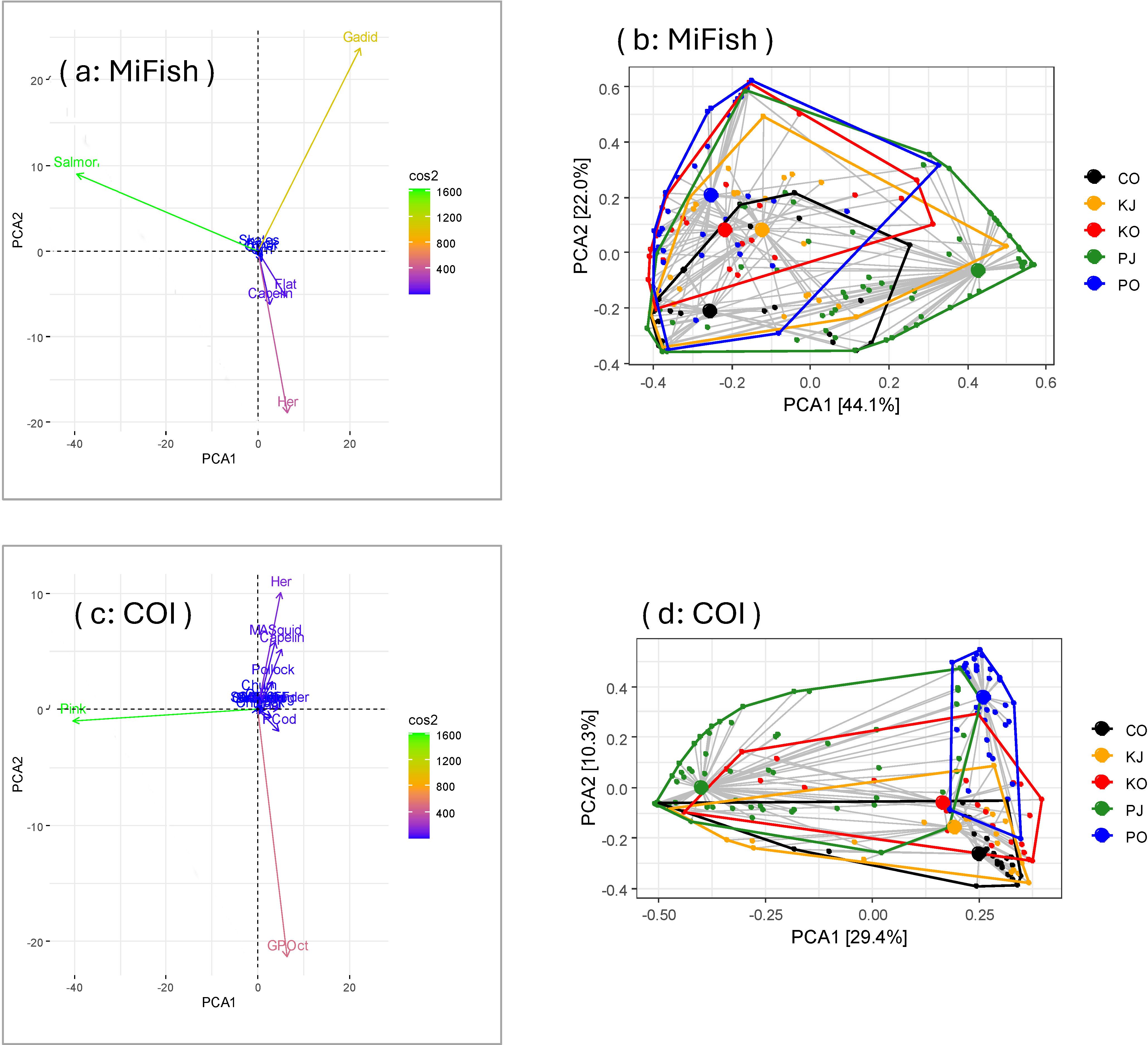
Figure 5. The first two principal components (PCA1, PCA2) summarizing prey composition in Steller sea lion scats from the Gulf of Alaska based on the 12S MiFish (A) and COI (C) (cytochrome c oxidase subunit I) results. 12S MiFish (B) and COI (D) group centroids and dispersion of prey data by region*season. Cos2 indicates how well the variable is represented on the first two principal components, and proportions on axes in (B, D) indicate the proportion of the variance explained by PCA1 and PCA2. Regions were C (Cook Inlet), K (Kodiak), P (Prince William Sound) for seasons J (July) and O (October). Prey taxa: GPOct, giant Pacific octopus; Pink, pink salmon; Her, herring; MASquid, magister armhook squid; PCod, Pacific cod; Flat, flatfish.
Because the COI results had fewer fish reads, we first pooled diet items into an “other” category with number of samples < 10, resulting in 17 prey groups. For the COI RRA results, the first principal component accounted for only 29.4% of the variation and up to 10 components were required to account for 93.0% of the variation (cumulative proportions improved gradually: to PCA 2, 5, 8 were 39.7%, 65.1%, 84.3%, respectively). Differences between the top components were due especially to pink salmon and giant Pacific octopus, and also herring, magister armhook squid and capelin (Figure 5C). PERMANOVA supported group differences (p = 0.001) and pairwise comparisons indicate all groups differed from each other in either means or dispersion (all p = 0.01). Dispersion differed among groups (p = 0.006) due to higher dispersion for PWS in July than Cook Inlet in October (p = 0.003) and Kodiak in July (p = 0.038; Figure 5D). Centroids appeared especially different between PWS in July and PWS in October than other groups, for the top two components (Figure 5D), but many other principal components captured variation among groups.
3.2.4 Sex differences
For 22 of 250 samples (8.8%), sex of host could not be determined, likely due to low quantities of DNA or high presence of PCR inhibitors. Our ability to assess sex differences was limited because male samples dominated the remaining 228 samples, likely due to preferential collection in male areas. Especially in July, areas with pups were not disturbed to minimize population impacts during the pupping season. Nearly all scats collected in July were from males (4.6% were from female) and 28.6% of scats collected in October were from females (40.6%, 20.0%, and 24.4% at Cook Inlet October, Kodiak October, and PWS October, respectively; n = 28 female samples total from October). Therefore, we examined sex differences in diet only for October samples.
Graphs of diet composition using 12S results suggested a potential greater use of salmon and sculpins by females and flatfishes by males (Figure 6A). Results were similar for COI, which also suggested potentially higher consumption of skates/dogfish and giant Pacific octopus by males compared to females (Figure 6C). Sex effect was strongest for Kodiak data (Figures 6B, D) and once group effect was included in PEMANOVA, sex effect was marginal in the 12S results (p = 0.081, given the small number of female samples) and supported in the COI data (p = 0.014), due especially to Kodiak and Cook Inet data (Figures 6B, D).
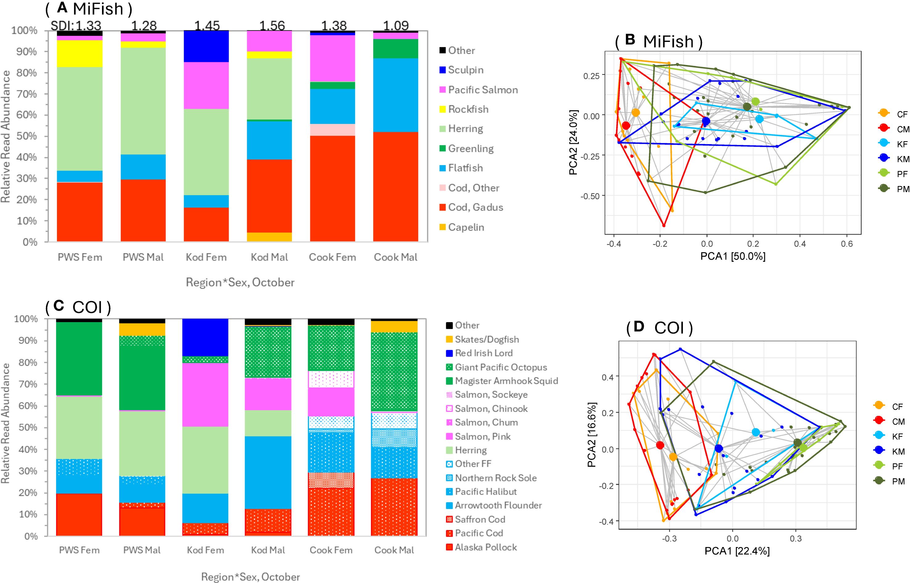
Figure 6. Sex differences in prey composition in Steller sea lion scats from the Gulf of Alaska collected in October, 2022–2023. Relative read abundance for prey items by region and sex for the two genes, (A) 12S MiFish and (C) COI. Group centroids and dispersion of prey data by region and sex for the two markers are in (B, D). Proportions on axes in (B, D) are proportions of the variance explained by the top two principal components (PCA1, PCA2). Regions were C, Cook Inlet (Cook); K, Kodiak (Kod); P, Prince William Sound (PWS) for sexes (F or M). SDI is Shannon Diversity Index, see Figure 3.
3.3 Parasitic worms and diet
We included all COI samples (n = 243) with >100 total assigned reads (n = 238), all of which also included SSL reads. Worms detected in these samples included parasitic round and tapeworms of the phylums Nematoda (order Rhabditida) and Platyhelminthes (genus Diphyllobothrium; Table 5). Polychaete worm (phylum Annelida, classes Polychaeta and Clitellata: including Lumbricillus pagenstecheri, genus Dasybranchus and genus Tomopteris) were detected in only 3 of 238 samples (1 male from Kodiak in October and 2 males from PWS in July). The parasitic worm community was dominated by Anisakis spp. roundworms (especially A. typica [55.5%] and A. simplex [24.3%]), and less so the tapeworm Diphyllobothrium tetrapterum (13.8%), together accounting for 93.5% of worm reads (Table 5).
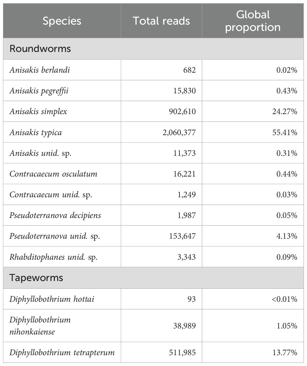
Table 5. COI results: Global parasitic worm composition in Steller sea lion scats from summer and fall in the Gulf of Alaska, 2022–2023, based on data from the cytochrome c oxidase subunit I (COI) gene. A non-parasitic roundworm (Rhabditophanes sp.) is also included.
Worm reads were common (86.97% of samples) but were lower in PWS in July (79.8%) and Cook Inlet in October (85.7%) compared to other groups (Kodiak July=93.9%, PWS October=92.7%, Kodiak October=100.0%; χ 24 df=11.01, p = 0.025). Dispersion of the worm community data varied among groups using RRA (betadisper, p < 0.001) and so PERMANOVA test results for mean differences in the worm community for groups were equivocal (Figure 7A). However, based on presence/absence data, the worm community in samples differed among groups (χ 2, all p < 0.05): Anisakis prevalence was lowest in Cook Inlet in October compared to other groups (76.7% vs. 87.1-100.0%). Prevalence of Diphyllobothrium was highest in Kodiak in October (68.0% vs. 34.5-50.0%). Pseudoterranova prevalence was highest in Cook Inlet in October (50.0% vs. 19.4-44.7%). Figure 7A). For parasite level index, 6 of 327 records had more worm reads than SSL reads, and these were changed to 1.0. Similar to the prevalence results, the Anisakis spp. level index varied significantly among groups with medians (first–third quartile) lowest for Cook Inlet Oct=0.009 (0.002–0.032) and PWS July=0.017 (0.004–0.058), and higher for Kodiak July=0.036 (0.008–0.128), Kodiak Oct=0.059 (0.010–0.132), and PWS Oct=0.081 (0.025–0.233; n = 218; Krusak-Wallis test p < 0.001). Too few samples containing other worm genera per group were available for group-specific levels. Diphyllobothrium spp. had a median index of 0.002 (0.001–0.011, n = 2 with 11 outliers above the third quartile) and Pseudoterranova spp. had a median index of 0.003 (0.001–0.014, n = 82 with 9 outliers).
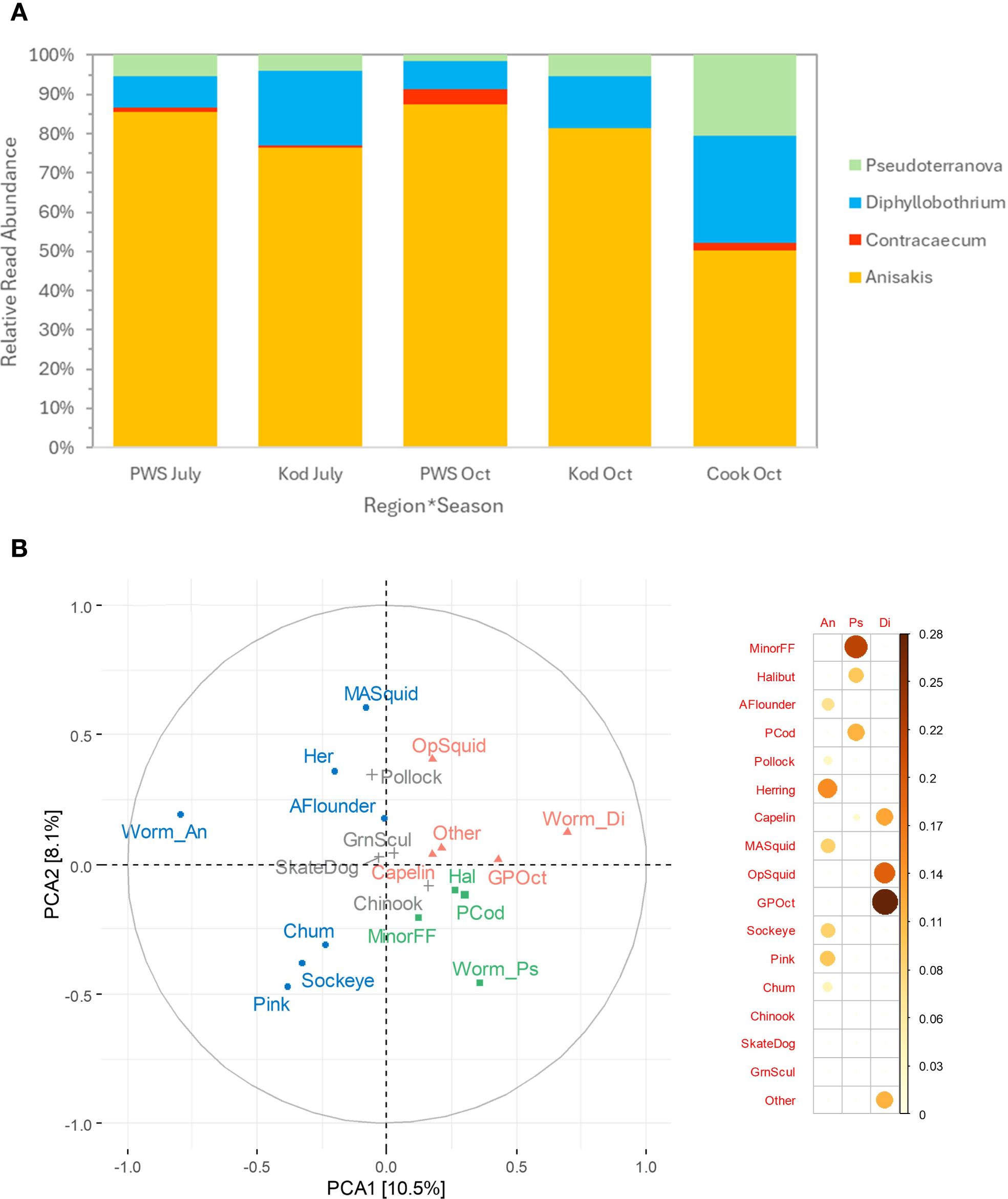
Figure 7. Composition of parasitic worms in Steller sea lion scats in the Gulf of Alaska by region*season (A) and diet (B). (A) Relative read abundance of the parasitic worm community by genus for regions Prince William Sound (PWS), Kodiak (Kod), and Cook Inlet (Cook) in July and October. (B) Worm composition in relation to diet for the three most prevalent genera: Anisakis (Worm_An), Diphyllobothrium (Worm_Di) and Pseudoterranova (Worm_Ps) shown by the two top principal components. Prey items positively associated with the three genera are color-coded based on Pearson correlations shown on the right (ranging to r = 0.28; larger orange to red circles indicated the most positively correlated).
Diet composition was significantly related to RRA of the three prominent worm genera (PERMANOVA, all p < 0.05). Diphyllobothrium RRA grouped best with giant Pacific octopus and opalescent squid; Pseudoterranova RRA grouped best with minor flatfishes, Pacific cod and halibut; and Anisakis RRA was positively associated with a different set of diet items, including herring and salmon (Figure 7B). Pearson correlation coefficients of the three worm genera and prey RRA per sample were not statistically significant (except Diphyllobothrium and giant Pacific octopus; p = 0.03, r = 0.279) but reflected well the principal components results (Figure 7B).
3.4 Saxitoxin prevalence, concentration, and associations with diet
With the minimum dilutions used in this study, the minimum detection limit for STX ranged between 2.6–6 ng/g. Of the 251 samples collected, 47 (18.7%) did not have STX measured due to the small sample volume such that all of the sample was needed for metabarcoding. Of the 204 remaining samples, STX was detected in 60.8% (95% CI: 54.1–67.5%) of samples, but prevalence varied among region*season (χ 24 df=34.42, p < 0.001). Prevalence was highest in PWS in July (83.3%), lowest in Cook Inlet in October (30.0%) and Kodiak in July (38.2%), and mid-range in Kodiak in October (56.5%) and PWS in October (57.6%). For the initial supplementary samples, STX was detected in 50.0% of 8 samples from the Kenai in winter (Jan–May 2017–2019) and 91.7% of 12 samples from SEAK in July 2016. For October samples, a sex difference in STX prevalence was not supported (females 59.1%, n = 22; males 44.3%, n = 61; p=0.34).
For samples in which STX was detected, concentrations of STX included outliers (maximum of 195 ng/g) creating heavy right tails and heterogeneity in variances among groups, precluding the use of linear models (Figure 8). Nonparametric tests indicated STX concentration varied significantly among groups in the 2022–2023 samples (Kruskal-Wallis test, p < 0.001, n = 124) due to higher concentrations for PWS July than other groups (pairwise comparisons using Wilcoxon rank sum exact test adjusted for multiple tests: all p < 0.021; Figure 8). For October samples, sex differences in STX concentrations were not supported (females: =13.94, n = 13; males: =30.61, n = 27; Krusak-Wallis test p < 0.076). Inclusion of supplemental datasets (samples <2022) supported higher STX concentrations in SEAK in July compared to Kodiak July and PWS October (pairwise comparisons using Wilcoxon rank sum adjusted for multiple tests: both p < 0.007; Figure 8).
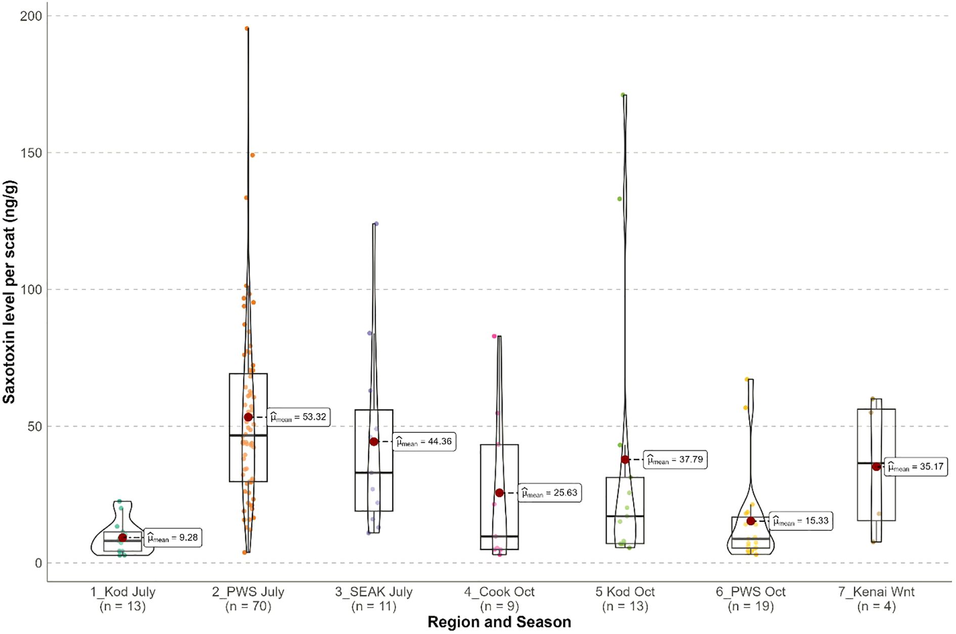
Figure 8. Saxitoxin levels (ng/g) measured in Steller sea lion scats from the Gulf of Alaska, 2016–2023. Regions were Kodiak (Kod), Prince William Sound (PWS), Southeast Alaska (SEAK), Cook Inlet (Cook) in seasons July and October; 8 samples from the Kenai in Winter (Jan–May, 2017–2019) were provided by the Alaska SeaLife Center. The violin plot shows medians (black line), intervals between lower to upper quartiles (boxed areas), data distributions, means (red circles) and outliers.
We assessed diet items associated with STX concentration separately for two region*season groups: PWS in July and October data pooled; Kodiak in July with low STX and a unique diet was not included. Outliers contained all salmon (~all pink) in PWS July (n = 4 highest), ~all giant Pacific octopus in Cook Inlet October and Kodiak October (n = 2 each), and either all pollock or ~all magister armhook squid in PWS October (n = 2, Figure 8). For PWS July (n = 69 with STX and COI results), 59.4% of samples were dominated (>50%) by pink salmon, and we removed the 3 highest outliers to prevent their undue influence on statistical tests. After grouping prey that was <5% of the PWS July diet into an “other” category, diet composition based on RRA varied with STX (PERMANOVA, p = 0.025); STX was positively associated with pink salmon in the first principal component but was also associated with pollock and less so, chum and magister armhook squid in the second component (STX contributed significantly, >20% each, to these 2 components, Figure 9A). For example, of 29 samples with STX > 50 ng/g, 72.4% contained nearly all pink salmon. However, the other eight samples had little or no pink salmon and were either dominated by chum salmon (n = 4, 13.8%) or pollock (also accompanied by small amounts of magister armhook squid; n = 4, 13.8%). Pearson correlations between RRA of diet items and STX were not significant, with r = 0.256 for pinks, 0.095 for pollock, -0.011 for chum, -0.082 for squid and -0.479 for “other”.
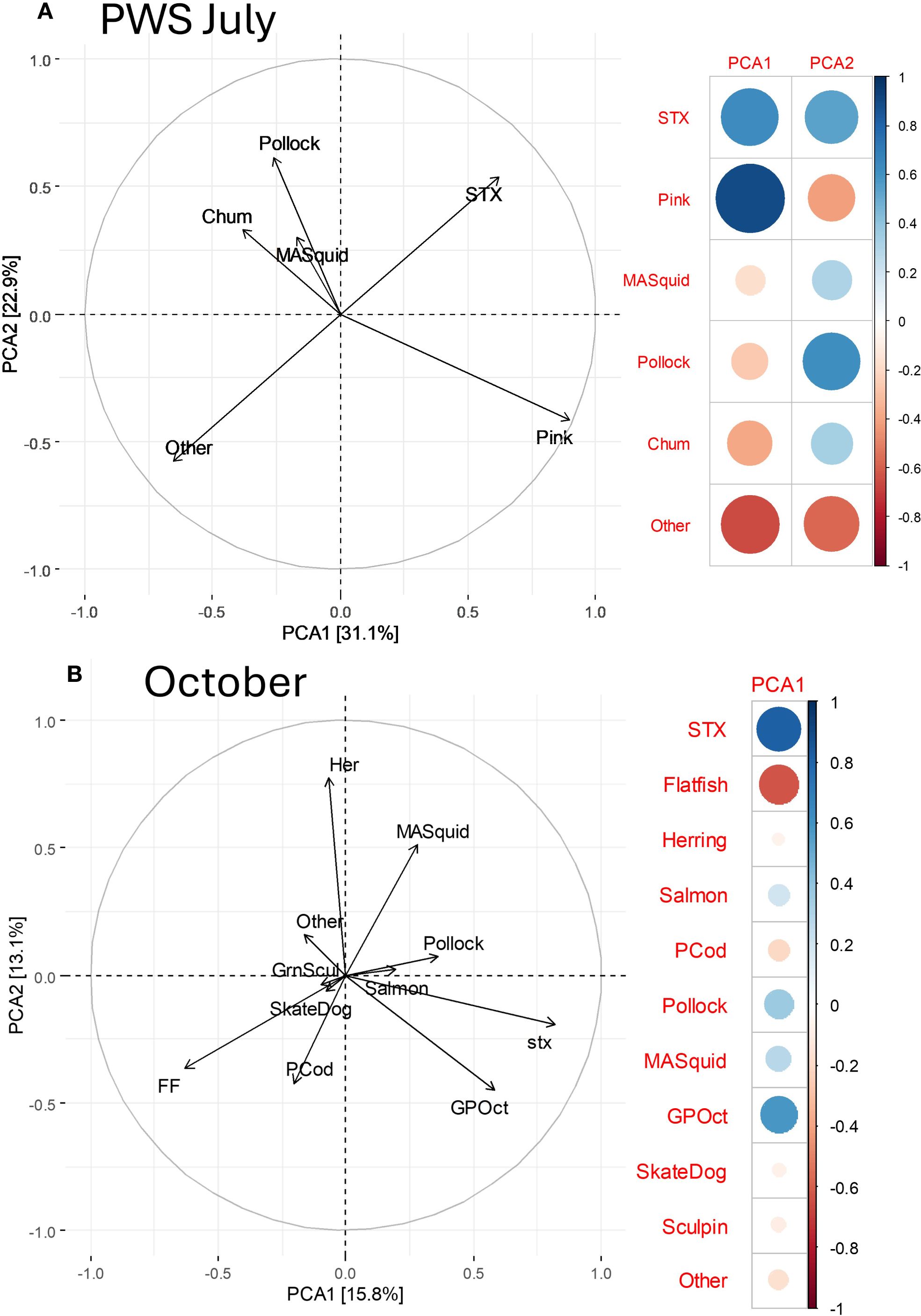
Figure 9. Saxitoxin (STX) levels in Steller sea lion scat in relation to diet composition in the Gulf of Alaska in July in Prince William Sound (PWS, A) and in October in all regions (B). Association of STX with diet items is apparent from the top two principal components (PCA1, PCA2; proportion of the variation explained by components is on the axes). STX loadings were high in PCA1 and PCA2 in (A) and in PCA1 in (B). The relative loadings (-1 to 1) of STX and prey groups for each principal component is shown on the right, where larger and darker blue is a stronger positive association and larger and darker red in a stronger negative association. Diet items abbreviations: Her, herring; MASquid, magister armhook squid; GPOct, giant Pacific octopus; PCod, Pacific cod; FF, flatfish; GrnSculp, Greenlings and Sculpins pooled, Greenlings and Sculpins pooled.
For October data, we removed the 2 outliers with STX >100 and pooled diet items into 10 groups (Figure 9B, n = 81). Diet composition in October based on RRA varied with STX (PERMANOVA, p = 0.003); STX contributed significantly to the first component and was positively associated with giant Pacific octopus and less so pollock, magister armhook squid and salmon (Figure 9B). Similarly, Pearson correlations between RRA of diet items and STX were also positive for giant Pacific octopus (0.386, p = 0.035), pollock (0.248), magister armhook squid (0.131), and salmon (0.094), and negative for other diet items, particularly flatfishes (-0.274), herring (-0.174) and Pacific cod (-0.113).
3.5 Seawater samples to assess SSL summer prey field
The 12S data resulted in an average of 1.8M reads per collection site for the 10m depth seawater samples (3 replicates per site summed; range = 787K–3.0M reads/site). Likely due to PCR inhibition, all three replicates at Seal Rocks resulted in no assigned reads, and 1–2 replicates produced no assigned reads for sites: Fish, Needle, Procession, and Rugged. Proportion unassigned averaged 62.1% over sites (excluding Seal Rocks; range = 32.8–98.8%). Total fish reads per site averaged 682K and was unusually low in Frederick Sound (6.2K) compared to other sites (range = 55.8K–1.4M). Due to high proportions of unassigned reads, proportion of total reads that were fish reads averaged 36.9% over samples [range=0.6%(in Frederick Sound)–67.0%].
RRA of fish in seawater samples for the 12S data was highest herring (45.4% of reads), followed by salmon (18.8%). Other fish groups included: gadids (9.5%), sand lance (6.6%), capelin (5.4%), sculpins (4.8%), rockfish (3.4%), greenlings (2.7%), pricklebacks (2.3%), sandfish (1.0%), and flatfishes (0.1%). Herring were detected throughout the entire study area (Figure 10). Similar to diet data, salmon proportions were especially high in PWS, and capelin and gadids were prevalent at sites in Kodiak (Figure 10A). Whereas the 10m depth samples at Seal Rocks contained no assigned reads, one sample from a surface bucket sample there contained 100% salmon. Diversity at 10m was highest in Kodiak area (sites: Marmot and Sea Otter) and northern SEAK, especially Graves Rocks. SEAK samples included more unique prey groups, such as sand lance, sandfish and pricklebacks (Figure 10A).
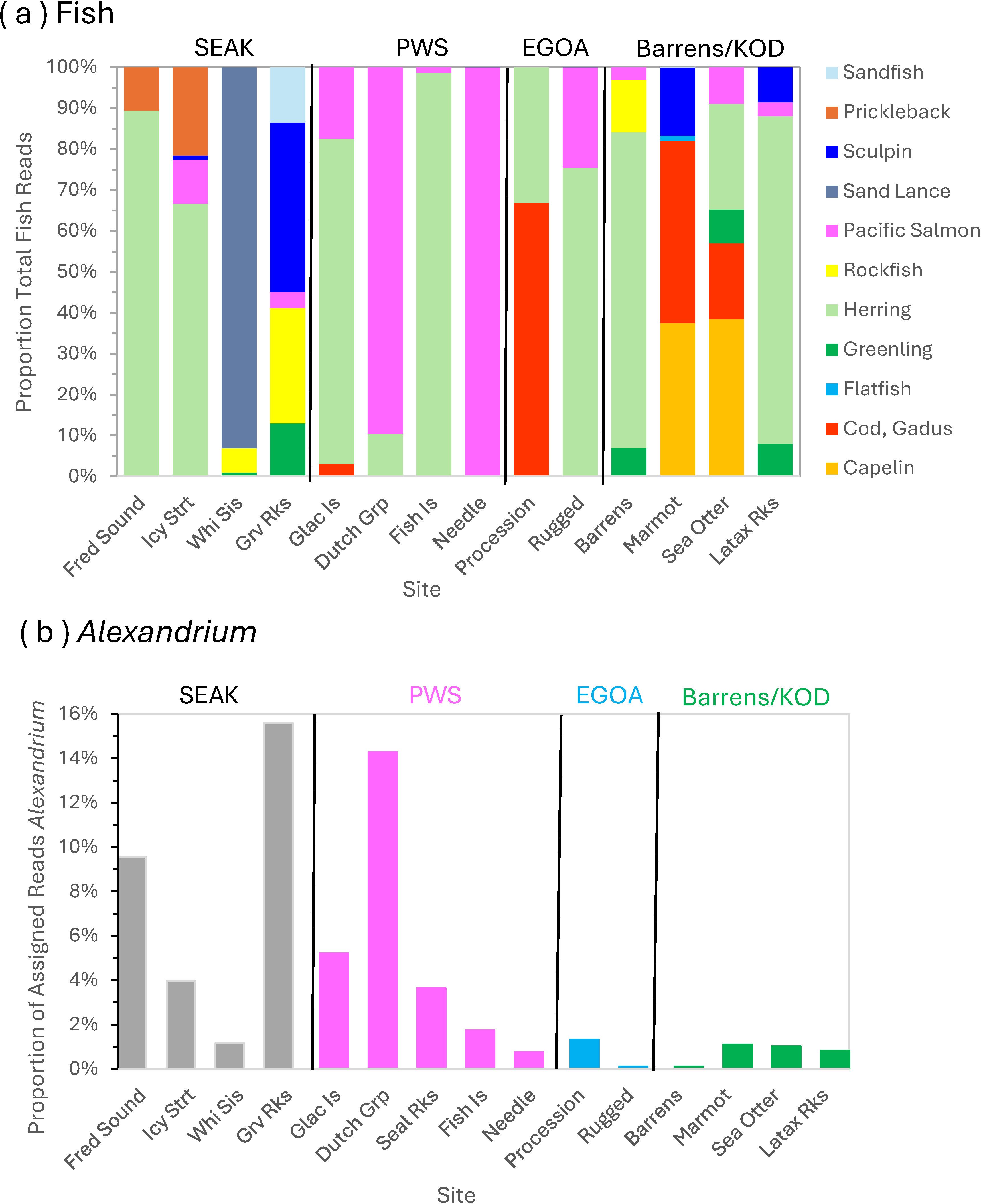
Figure 10. Geographic variation in (A) fish composition and (B) abundance of Alexandrium spp. in the Gulf of Alaska in July, 2023, from Southeast Alaska (SEAK) to Kodiak Island (KOD) using eDNA in seawater collected at 10m water depth. See Figure 1 for site locations. PWS, Prince William Sound; EGOA, eastern Gulf of Alaska region, including the Kenai Peninsula. (A) based on 12S MiFish results, (B) based on COI results.
The COI data resulted in very few fish reads per site (average n = 122, range = 10–399) and overall (n = 1,707), instead, plankton reads, especially copepods and bloom-forming and/or toxic diatom or dinoflagellates, were most prevalent. Of 4.6M assigned reads, the second highest proportion of reads were from Alexandrium spp., a toxic dinoflagellate producing STX (6% of assigned reads). The proportion of total reads assigned to Alexandrium spp. varied among sites (χ 2, p < 0.001) and was highest in SEAK and PWS, specifically at Graves Rocks, Dutch Group, and Frederick Sound in July 2023 at 10m depth (9–16%, Figure 10B). Fish reads were too few to assess geographic diversity with COI, but COI results indicated red Irish lord may be an important sculpin at Graves Rocks, Marmot Island, and Latax Rocks in the 12S results (Figure 10A). Black rockfish occurred at Graves Rock, and most salmon detected were pink salmon throughout the study area (79.6% pink, 20.4% chum, n = 353).
4 Discussion
In this study we documented several important insights into recent SSL diet composition in the Gulf of Alaska, including: (1) the importance of cephalopods in the diet especially magister armhook squid in PWS and giant Pacific octopus in Kodiak and Cook Inlet, (2) consumption of a new cephalopod, opalescent or market squid, that moved into the Gulf of Alaska from California during recent warm water events, (3) the potential shift from dominance of pollock to more salmon, capelin, herring, arrowtooth flounder and Pacific cod observed in other studies during population recovery from 1999 to 2009 (McKenzie and Wynne, 2008; Sinclair et al., 2013) is also suggested in our dataset, (4) the identification of pink salmon as the salmon species most consumed by SSL in both seasons in our study area (see also Tollit et al., 2009), and (5) a needed re-examination of SSL diet composition in PWS not provided since the 1970s (Pitcher, 1981) indicated the importance of pink salmon in summer and of herring, magister armhook squid, and pollock in fall in 2022–2023 (Figures 3, 4). Because PCR results indicated that the majority of our scat samples were from males (~95% in July and 71% in October), our study specifically addressed male diet composition. For October diet for which both sexes provided data, male diet was similar to female diet, especially in the deep waters of Prince William Sound, but for areas with access to shallower water over the continental shelf (Kodiak and Cook Inlet), males consumed more demersal fish than females. Female summer diet was not addressed by our study.
The use of two mitochondrial gene regions (12S and COI) improved our understanding of diet patterns. Both genes produced very similar diet data results and differed most in taxonomic resolution of results. The shorter gene region utilized by the 12S rRNA MiFish-U primer excels at detecting fish taxa (Miya et al., 2015), our target taxa of interest, but allowed mostly genus-level resolution of taxa in our study. Larger gene regions like COI often provide high taxonomic resolution across the food web but can lead to reduced efficiency of PCR yielding a product that may be prone to sequencing errors resulting in lower read counts or poor-quality reads (reviewed by Bylemans et al., 2018). The COI gene also has a high degree of degeneracy which can lead to species-specific primer-template mismatches resulting in PCR bias that may hinder analyses (Leray et al., 2013). While the 12S gene region produced high numbers of fish reads, we found the COI gene region valuable for species-level resolution for fish and cephalopod taxa in SSL scat samples and for addressing other taxa of interest (e.g., parasitic worms in scats and saxitoxin-producing dinoflagellates in seawater).
Consumption of cephalopods by SSL is well documented (Pitcher, 1981; Trites et al., 2007; Goto et al., 2017) but determining rates of consumption by hard parts is challenging, as some species may not be detectable in scats, and under-representation in scats and over-representation in stomachs is expected due to regurgitation and retention of cephalopod beaks in the stomach (Pitcher, 1981; Sinclair and Zeppelin, 2002; reviewed by Tollit et al., 2009). DNA provides the best means of assessing cephalopods in the diet and was used to determine their importance in SSL diets in the Aleutians, where especially giant Pacific octopus was consumed (Tollit et al., 2017). Cephalopods were among the top diet items consumed in October in our study area: relative read abundances were >28% for magister armhook squid and giant Pacific octopus in PWS and Kodiak/Cook Inlet, respectively (Figure 4). Trends of cephalopod consumption by SSL in Alaska may be useful to monitor status of these poorly studied populations in Alaska, as cephalopod populations are increasing globally perhaps related to warming oceans and/or global depletion of fish stocks (Doubleday et al., 2016). Squids were important prey in PWS in the late 1970s (Pitcher, 1981) and in SEAK in the 1990s, where magister armhook squid was identified as an important prey (Trites et al., 2007; also in Japan: Goto et al., 2017). Magister armhook squid is very abundant in the North Pacific, is an important food of northern fur seals (Sinclair et al., 1994; Antonelis et al., 1997) and is considered an energy-rich prey (Perez, 1994).
The regional difference in cephalopods consumed in our study area may reflect regional differences in habitats or foraging behavior, such as more pelagic/benthopelagic, vertically-migrating prey in the deeper waters of PWS (e.g., magister armhook squid was often consumed with other pelagic species, pollock and herring; Figure 2) compared to benthic foraging for giant Pacific octopus (often consumed with arrowtooth flounder and Pacific cod; Figure 2) in Kodiak/Cook Inlet with a broad, shallow continental shelf. This may also explain the regional difference in gadids with pollock consumed in PWS versus Pacific cod in Kodiak/Cook Inlet (Figure 4).
Market or opalescent squid are highly abundant in the California Current System, currently sustaining the largest fishery in the U.S. and serving as a key prey source for marine apex predators in that region (Morejohn et al., 1978). Market squid have periodically expanded their range northward from the California Current System into the Gulf of Alaska, most recently during warm water events in the early 2000s and again in 2015 (Burford et al., 2022). Market squid, including spawning, were observed from 2015–2016 in SEAK (Dixon Entrance, Little Port Walter, Sitka Sound) and off Katmai in 2017 (Eiler, 2021; Burford et al., 2022). We detected market squid in 12 scat samples (from 11 male and 1 female SSL) from PWS in July and October 2022 (10% of the PWS samples in that year). However, this squid occurred in low proportions in these samples, averaging <1% of total fish/cephalopod reads (ranging from <1.0% to 8.3% of total prey reads among samples). Continued sampling of SSL scats may indicate whether this latest range shift is temporary (Cavole et al., 2016) or indicative of a longer residency for this species in the Gulf of Alaska.
Our results support the findings of two recent SSL diet studies which suggested a shift in recent years from dominance of pollock (observed in the late 1970s through the 1990s; Pitcher, 1981; Sinclair and Zeppelin, 2002) to inclusion of more forage fishes and other prey in Kodiak/Cook Inlet (McKenzie and Wynne, 2008; Sinclair et al., 2013). Pollock detections were particularly low in our samples. If the proportions of the two gadid species from the COI data were applied to the 12S proportions, proportions of pollock in the fish diet were small in Kodiak and Cook Inlet (<0.1–4.5%) and 22.5–25.7% in PWS. Instead, Pacific cod made up 22.0–26.4% of the diet in Kodiak and 51.5% in Cook Inlet. We may expect pollock detections in particular to be lower in studies based on DNA in soft matrix versus hard parts because pollock detections are biased high in hard parts data due to longer retention times and higher recovery rates for prey with sturdy bones such as pollock, so that more data and meals are included for those species compared to data from soft matrix only (Tollit et al., 2003; Tollit et al., 2009; see also Maniscalco, 2023 which detected pollock only in hard parts and in high numbers but not in DNA-based data). Because of these biases, an examination of hard parts from the scat samples used in our study would provide verification that pollock prevalence was lower in our recent study compared to diet studies during the population decline based on hard parts, as was also found by McKenzie and Wynne (2008) and Sinclair et al. (2013). Our finding that Pacific cod was consumed more than pollock in Kodiak/Cook Inlet was also in agreement with the more recent hard part studies. Use of Pacific cod may have increased as the use of pollock decreased in the Kodiak/Cook Inlet region in the 2000s compared to the 1990s (Region 1; Figure 5 in Sinclair et al., 2013). In northern Kodiak from 1999–2005 in the fall, the proportions of the diet that were pollock and Pacific cod were similar (ranging from 2.2–13.2% and from 3.3–14.1% among years, respectively; Appendix 1 in McKenzie and Wynne, 2008).
We suspect that high diet diversity and incidence of forage fish in our sample reflects a true pattern, in agreement with McKenzie and Wynne (2008) and Sinclair et al., 2013, despite differences in methodology. Prey detections can be much higher in hard parts data and DNA-based data can yield some new diet items and increase species richness (Tollit et al., 2009). However, studies comparing results for the different methodologies often yield similar or near identical diet compositions (Tollit et al., 2009; Thomas et al., 2022), even for prey such as salmon with more fragile bones (Thomas et al., 2022). The use of hard parts may provide unique information pertaining to diet such as prey sizes or age-classes (Tollit et al., 2004; Zeppelin et al., 2004; Thomas et al., 2022), but recent reviews by pinniped diet specialists compared results from DNA metabarcoding RRA to hard parts biomass reconstruction (considered the best current method; Tollit et al., 2015) and suggested that moving to DNA-based-only data studies may now be more efficient as metabarcoding provides better taxonomic resolution and produces similar results with less effort (Thomas et al., 2022).
Capelin made up a higher proportion of Kodiak summer diet than reported in recent studies: 42.0% and 44.8% based on 12S and COI, respectively (Figures 3, 4). Capelin is an important energy dense prey for SSL in summer in this region and historically (Pitcher, 1981; McKenzie and Wynne, 2008). Reduced capelin in the diet of SSL in winter coincided with negative population effects during the Pacific Marine Heatwave of 2014–2016 in the Kenai region (Maniscalco, 2023). Curiously, sand lance was nearly absent from our samples, occurring as a rare diet item (Figures 3, 4). Sand lance occurred in 14 samples and all but 1 sample with ~100% of reads sand lance (a male in PWS in July) contained <5% of reads sand lance per sample, suggesting these were potentially secondary prey ingested by salmon, gadids or flatfishes. Sand lance were the most abundant diet item in scats in Kodiak from 1999–2005 (McKenzie and Wynne, 2008), so their near absence in our samples was unexpected.
Pink salmon are the most important salmon species for SSL in our study area (60.6% of the diet in PWS in July, and up 17.1% in other regions*seasons), followed distantly by chum salmon (14.0% in PWS in July and up to 2.0% in other groups; Figure 4). Other species were <1% of the diet, except chinook in Cook Inlet in October (3.4%) and sockeye in PWS in July (2.2%). These are higher proportions of pinks than previously reported for salmon species consumed by Alaskan SSL outside of the PWS–Kodiak region (pink 39%, chum 29%, chinook 14%; Tollit et al., 2009). Although pink salmon may show alternating years of strong cohorts (Ruggerone et al., 2023), we observed pink salmon were high in PWS July diet in both years (detected in 63.6% and 76.5% of samples with >1K fish reads in 2022 and 2023, respectively). High abundance of this species in PWS and elsewhere may account for its’ dominance in the diet we observed. Pink salmon are presently the most abundant salmon species in the North Pacific accounting for 70% of adult returning salmon, with large population increases (>65%) observed since the shift to warm conditions in 1976–77 (Ruggerone et al., 2010, Ruggerone et al., 2023). Pink salmon are abundant in PWS, where large pink salmon hatcheries also occur (Ward et al., 2017). Salmon consumption by SSL in Alaska varies seasonally and regionally, although it is usually highest in the spring and summer (Pitcher, 1981; Sinclair and Zeppelin, 2002) or fall depending on spawning behavior (Tollit et al., 2015). A broader sampling of localities and months may indicate a greater reliance on other species of salmon than found by our study (Tollit et al., 2009).
Male and female diets differed in October in Kodiak and Cook Inlet with males consuming more benthic prey (giant Pacific octopus, cods and flatfishes) and females consuming more pelagic prey, (salmon and herring) and sculpins, particularly red Irish lord, a fish often occurring nearshore in shallower water or the intertidal zone (Figure 6). Sex differences in diet composition were not apparent in PWS, where deep waters nearshore may favor pelagic foraging for both sexes (Figure 6). Similar to our results for PWS, sex differences in diet were not observed for SSL in Washington based on year-round data (Lewis, 2022). The ability to use DNA to determine sex of the host in scat samples improves our understanding of demographic aspects of diet and other demographic patterns (e.g., sex-specific site-use; Lewis, 2022; Gard et al., 2024). Prior to the development of DNA techniques, sex segregation of SSL at rookeries during the breeding season allowed sex-specific diet to be assessed during that season at rookeries. Males consumed fewer salmon and more pollock, flatfishes and rockfish than females at the large Forrester Island rookery in SEAK in June–July in the 1990s (Trites and Calkins, 2008). Adult male SSL are much larger than females (2.5 times larger in average body mass at age 12+; Winship et al., 2001) and therefore have higher aerobic dive limits than females that may allow them to efficiently exploit more habitats and water depths in variable environments (Schreer and Kovacs, 1997).
We documented several potential stressors related to diet consumption for SSL including evidence that SSL may be chronically exposed to STX at low concentrations throughout our study area. Current information on STX exposure for SSL in Alaska using a larger sample size was needed to provide a baseline for future monitoring of this growing threat (Lefebvre et al., 2016). The threat of harmful algal blooms to Alaskan marine mammals is well documented (Lefebvre et al., 2016). We found higher prevalence and concentrations of STX than previously reported for SSL fecal samples collected in Alaska from 2004–2013 (%positive=10%, maximum concentration=7 ng/g, n = 42; Lefebvre et al., 2016). In our 2022–2023 samples, 60.8% of scats contained STX > 2.6–6 ng/g and concentrations ranged from means of 9.28 ng/g to 53.32 ng/g among regions and season, with 5 samples containing >100 ng/g and a maximum concentration of 195 ng/g observed (Figure 8). It cannot be determined whether this may indicate that STX exposure has increased in Alaskan SSL over the last decade, but continued sampling would be useful to detect temporal trends. The samples in Lefebvre et al. (2016) were from fresh carcasses rather than scats collected from the ground as in our study. We consider these samples comparable because we included only fresh scats frozen within 6 hours of collection to minimize potential changes in toxin concentrations due to environmental exposure after deposition (Akmajian et al., 2017). The concentrations of STX in scats that we observed were similar to those for SSL in Washington (%positive=45% ranging ~20–75% among seasons*locations, mean concentrations=~25–50 ng/g among season*locations, maximum concentration=273 ng/g; Akmajian et al., 2017). Finally, our data indicated a link between STX and salmon consumption, especially in July, and with giant Pacific octopus, magister armhook squid, and pollock consumption (Figure 9). Consumption of pollock was also associated with higher STX exposure in SSL in Washington (Akmajian et al., 2017).
Although these concentrations are higher than previously reported, they were well below the seafood safety regulatory limit of 800 ng/g. Instead, in Alaska, Pacific walrus (Odobenus rosmarus divergens), humpback whales (Megaptera novaeangliae) and bowhead whales (Balaena mysticetus) may be more at risk of acute health effects as indicated by higher measured concentrations in those species (Lefebvre et al., 2016, Lefebvre et al., 2022). However, the effects of chronic exposure of STX on marine mammals are not well studied and may add stress to at-risk populations. STX production is expected to be highest when water warming in summer promotes algal blooms (Anderson et al., 2021); exposure was highest in July in our study and in spring in Washington (Akmajian et al., 2017). However, as in Washington, exposure occurred year-round, outside the bloom time, and may be due to resuspension of dormant Alexandrium cysts residing in the benthos (reviewed by Akmajian et al., 2017). The highest concentrations of STX observed were in PWS and in northern SEAK (from a supplemental sample collected at Graves Rock during July 2016, during the peak of the North Pacific Marine Heatwave of 2014–2016 in that area; Hastings et al., 2023a). These areas also contained the highest number of reads of Alexandrium spp. at 10m depth in 2023 (Figure 10a). The marine ecosystem east of Cook Inlet (including SSL in PWS and SEAK) was especially impacted by the Pacific Marine Heatwave, despite the presence of warm water throughout the Gulf, suggesting oceanographic and habitat characteristics specific to these regions may exacerbate deleterious effects of warming on the food web (Suryan et al., 2021; Hastings et al., 2023a). More study is needed to determine if increased risk of STX exposure is an additional stressor with warming particularly in these regions.
COI offered an opportunity to document intestinal parasitic worms, a second potential diet-related stressor for SSL that has been minimally studied. As expected in marine mammals (Dailey, 2001), we found high incidence of worm infections, especially Anisakis spp. roundworms (range 76.7–100% among region*seasons) which, together with Diphyllobothrium spp. tapeworms (34.5–68.0%), and Pseudoterranova spp. roundworms (19.4–50.0%), made up >99% of worm reads. Important species identified included A. typica, A. simplex, and D. tetrapterum (Table 5). Other than D. tetrapterum and Contracaecum osculatum (Shults, 1986), the species in Table 5 have not previously been identified for SSL in Alaska. Identifications of species making up <1% of total parasitic worm reads in Table 5 should be treated cautiously as small numbers of false positives may occur, but the COI gene is considered a preferred method for nematode identification (Mejías-Alpízar et al., 2024). Similar to our results, Anisakis spp. were the most prevalent parasite in SSL prey in Alaska, with Pseudoterranova spp. occurring less frequently (Moles and Heintz, 2007).
Anisakis spp. prevalence and levels were highest in PWS and Kodiak in October and for these groups the highest prevalence of other parasitic worm genera was also observed (Pseudoterranova spp. in PWS, and Diphyllobothrium in Kodiak). Nematode infection rates in SSL prey were lower in SEAK where SSL numbers were increasing than in the Aleutian Islands where they were decreasing, perhaps due to different prey consumed (Moles and Heintz, 2007). Benthic-associated fishes (Atka mackerel Pleurogrammus monopterygius, Pacific cod, pollock, flatfishes such as arrowtooth flounder) tended to have highest rates of Anisakis spp. and Pseudoterranova spp. infections, although Anisakis spp. infections occurred in all species studied (Moles and Heintz, 2007). Parasitic worm prevalence and levels in scats are not expected to be directly related to recent feeding events, unless recent meals mirror general feeding patterns. Assuming that, our assessment of worm levels and diet composition in scats suggested positive associations between Diphyllobothrium and giant Pacific octopus, Pseudoterranova and flatfishes, and Anisakis and a different prey assemblage, including herring and salmon (Figure 7B). This may indicate that increased consumption of herring, diverse flatfishes in Cook Inlet, and giant Pacific octopus may increase parasitic worm exposure for SSL in October. Although specific parasites harbored by giant Pacific octopus in Alaska require study, octopus are important vectors for the transmission of cestodes in the food web (Roumbedakis et al., 2018; Tedesco et al., 2020).
Data from seawater samples to assess the prey field for SSL in July in conjunction with scat collections suggested SSL were foraging regionally on available prey, with pink salmon prevalent in the PWS and capelin, cods, and sculpins in Kodiak (Figure 10). Multiple diet studies demonstrate that SSL are generalist predators feeding on prey that is plentiful regionally and seasonally based on seasonal, geographic and behavioral knowledge of SSL prey (Pitcher, 1981; Sinclair and Zeppelin, 2002) but rarely have the diet and prey field both been directly assessed (Womble and Sigler, 2006). The lack of fish diversity in PWS and the eastern Gulf of Alaska sites was in contrast to higher diversity in SEAK and at the Barren Islands and Kodiak (Figure 10). The prevalence of herring in seawater samples but not in the July diet data suggests herring are occurring in the environment in high numbers across a broad area but are not as accessible to SSL, perhaps due to movements of herring that reduce predictability of finding this prey. In PWS, herring spawn from late March to April, and many herring schools move from coastal spawning areas from late April-July out into the Gulf of Alaska, with some schools highly mobile outside the spawning time (Bishop and Eiler, 2018).
Results from our pilot survey suggest this may be a useful and efficient method for monitoring nearshore prey in conjunction with SSL surveys. Further study is needed to address potential methodological issues for prey sampling such as effects of water depth, water volume, and numbers of replicate samples required for adequate numbers of reads for different gene regions. Our results suggest ~5L samples per site per water depth may be adequate for fish detections with the 12S rRNA MiFish-U gene region although a larger volume of seawater could be tested to determine gains in information possible. Use of the COI gene was informative across the food web, especially lower trophic levels, but for targeting information on fish biodiversity sampling modifications will be required (e.g., larger seawater volumes, smaller membrane pore size to capture a larger portion of the particulate) to increase detections of higher trophic levels.
Data availability statement
The data supporting the findings of this study, including raw sequence data (fastq), are publicly available in the Dryad Digital Repository. The dataset can be found here: https://doi.org/10.5061/dryad.s7h44j1md.
Ethics statement
This animal study was approved by the Alaska Department of Fish and Game Institutional Animal Care and Use Committee and US National Marine Fisheries Service Permit #22298. The study was conducted in accordance with local legislation and institutional requirements.
Author contributions
KH: Methodology, Funding acquisition, Investigation, Conceptualization, Writing – original draft, Data curation, Formal Analysis, Project administration, Writing – review & editing. MR: Project administration, Conceptualization, Supervision, Writing – original draft, Investigation, Funding acquisition, Writing – review & editing. LC: Investigation, Writing – review & editing, Formal Analysis, Data curation, Writing – original draft. EB: Formal Analysis, Writing – original draft, Data curation, Methodology, Writing – review & editing, Investigation. KL: Supervision, Methodology, Writing – review & editing, Investigation, Funding acquisition, Writing – original draft, Project administration, Data curation.
Funding
The author(s) declare financial support was received for the research and/or publication of this article. Funding for this research was provided by the State of Alaska, a NOAA Fisheries Species Recovery Grant to the Alaska Department of Fish and Game, NA22NMF4720104 and the NOAA National Center for Coastal Ocean Science ECOHAB grant (NA20NOS4780195). This is ECOHAB contribution #1138.
Acknowledgments
We are particularly grateful for guidance, discussions and/or reviews of this research by A. Thomas, D. Tollit, A. Akmajian, Z. Lewis, C. Clark, E. D’Agnese, D. Rosen, T. Zeppelin, and L. Jemison. We also especially thank M. Akers for laboratory expertise, J. Maniscalco (Alaska SeaLife Center) for sharing samples from the Kenai Peninsula area for saxitoxin research, and the Alaska Department of Fish and Game’s Gene Conservation Laboratory for assisting with our project: S. Gilk-Baumer, Z. Grauvogel, H. Hoyt and C. Jalbert.
Conflict of interest
Authors EB was employed by Ocean Associates, Inc.
The remaining authors declare that the research was conducted in the absence of any commercial or financial relationships that could be construed as a potential conflict of interest.
Generative AI statement
The author(s) declare that no Generative AI was used in the creation of this manuscript.
Any alternative text (alt text) provided alongside figures in this article has been generated by Frontiers with the support of artificial intelligence and reasonable efforts have been made to ensure accuracy, including review by the authors wherever possible. If you identify any issues, please contact us.
Publisher’s note
All claims expressed in this article are solely those of the authors and do not necessarily represent those of their affiliated organizations, or those of the publisher, the editors and the reviewers. Any product that may be evaluated in this article, or claim that may be made by its manufacturer, is not guaranteed or endorsed by the publisher.
References
Acevedo-Whitehouse K. and Duffus A. L. J. (2009). Effects of environmental change on wildlife health. Philos. Trans. R. Soc B Biol. Sci. 364, 3429–3438. doi: 10.1098/rstb.2009.0128
Adams C. F., Foy R. J., Johnson D. S., and Coyle K. O. (2008). Seasonal changes in pelagic fish biomass around the Chiswell Island Steller sea lion rookery in 2003. Fish. Res. 93, 179–185. doi: 10.1016/j.fishres.2008.04.003
Akmajian A. M., Scordino J. J., and Acevedo-Gutiérrez A. (2017). Year-round algal toxin exposure in free-ranging sea lions. Mar. Ecol. Prog. Ser. 583, 243–258. doi: 10.3354/meps12345
Amaya D. J., Miller A. J., Xie S., and Kosaka Y. (2020). Physical drivers of the summer 2019 North Pacific marine heatwave. Nat. Commun. 11, 1903. doi: 10.1038/s41467-020-15820-w
Anderson M. J. (2001). A new method for non-parametric multivariate analysis of variance. Austral Ecol. 26, 32–46. doi: 10.1111/j.1442-9993.2001.01070.pp.x
Anderson M. J. (2006). Distance-based tests for homogeneity of multivariate dispersions. Biometrics 62, 245–253. doi: 10.1111/j.1541-0420.2005.00440.x
Anderson D. M., Fachon E., Pickart R. S., Lin P., Fischer A. D., Richlen M. L., et al. (2021). Evidence for massive and recurrent toxic blooms of Alexandrium catenella in the Alaskan Arctic. PNAS 118, e2107387118. doi: 10.1073/pnas.2107387118
Anderson P. J. and Piatt J. F. (1999). Community reorganization in the Gulf of Alaska following ocean climate regime shift. Mar. Ecol. Prog. Ser. 189, 117–123. doi: 10.3354/meps189117
Ando H., Mukai H., Komura T., Dewi T., Ando M., and Isagi Y. (2020). Methodological trends and perspectives of animal dietary studies by noninvasive fecal DNA metabarcoding. Environ. DNA 2, 391–406. doi: 10.1002/edn3.117
Antonelis G. A., Sinclair E. H., Ream R. R., and Robson B. W. (1997). Inter-island variation in the diet of female northern fur seals (Callorhinus ursinus) in the Bering Sea. J. Zool. Lond. 242, 435–451. doi: 10.1111/j.1469-7998.1997.tb03847.x
Arfin N. A., Barua A., Datta S. K., Ahmed S., and Ahmed M. S. (2023). Genetic diversity of cephalopods (Mollusca: Cephalopoda) from Bangladesh waters based on COI and 16S rRNA genes. Thalassas 39, 1199–1205. doi: 10.1016/j.jafr.2025.101683
Arimitsu M. L., Piatt J. F., Hatch S., Suryan R. M., Batten S., Bishop M. A., et al. (2021). Heatwave-induced synchrony within forage fish portfolio disrupts energy flow to top pelagic predators. Glob. Change Biol. 27, 1859–1878. doi: 10.1111/gcb.15556
Bakker J. D. (2024). Applied multivariate statistics in R (University of Washington Pressbooks). Available online at: https://uw.pressbooks.pub/appliedmultivariatestatistics/ (Accessed September 30, 2025).
Barkhordarian A., Nielsen D. M., and Baehr J. (2022). Recent marine heatwaves in the North Pacific warming pool can be attributed to rising atmospheric levels of greenhouse gases. Commun. Earth Environ. 3, 131. doi: 10.1038/s43247-022-00461-2
Baylis A. M. M., Orben R. A., Arnould J. P. Y., Christiansen F., Hays G. C., and Staniland I. J. (2015). Disentangling the cause of a catastrophic population decline in a large marine mammal. Ecology 96, 2834–2847. doi: 10.1890/14-1948.1
Beukhof E., Dencker T. S., Pecuchet L., and Lindegren M. (2019). Spatio-temporal variation in marine fish traits reveals community-wide responses to environmental change. Mar. Ecol. Prog. Ser. 610, 205–222. doi: 10.3354/meps12826
Birnie-Gauvin K., Peiman K. S., Raubenheimer D., and Cooke S. J. (2017). Nutritional physiology and ecology of wildlife in a changing world. Conserv. Physiol. 5, cox030. doi: 10.1093/conphys/cox030
Bishop M. A. and Eiler J. H. (2018). Migration patterns of post-spawning Pacific herring in a subarctic sound. Deep-Sea Res. II Top. Stud. Oceanogr. 147, 108–115. doi: 10.1016/j.dsr2.2017.04.016
Bolyen E., Rideout J. R., Dillon M. R., Bokulich N. A., Abnet C. C., Al-Ghalith G. A., et al. (2019). Reproducible, interactive, scalable, and extensible microbiome data science using QIIME 2. Nat. Biotechnol. 37, 852–857. doi: 10.1038/s41587-019-0209-9
Bond N. A., Cronin M. F., Freeland H., and Mantua N. (2015). Causes and impacts of the 2014 warm anomaly in the NE Pacific. Geophys. Res. Lett. 42, 3414–3420. doi: 10.1002/2015GL063306
Boyse E., Robinson K. P., Beger M., Carr I. M., Taylor M., Valsecchi E., et al. (2024). Environmental DNA reveals fine-scale spatial and temporal variation of marine mammals and their prey species in a Scottish marine protected area. Environ. DNA 6, e587. doi: 10.1002/edn3.587
Bronson F. H. (1985). Mammalian reproduction: An ecological perspective. Biol. Reprod. 32, 1–26. doi: 10.1095/biolreprod32.1.1
Burford B. P., Wild L. A., Schwarz R., Chenoweth E. M., Sreenivasan A., Elahi R., et al. (2022). Rapid range expansion of a marine ectotherm reveals the demographic and ecological consequences of short-term variability in seawater temperature and dissolved oxygen. Am. Nat. 199, 523–550. doi: 10.1086/718575
Bylemans J., Gleeson D. M., Hardy C. M., and Furlan E. (2018). Towards an ecoregion scale evaluation of eDNA metabarcoding primers: A case study for the freshwater fish biodiversity of the Murray-Darling Basin (Australia). Ecol. Evol. 8, 8697–8712. doi: 10.1002/ece3.4387
Callahan B. J., McMurdie P. J., Rosen M. J., Han A. W., Johnson A. J. A., and Holmes S. P. (2016). DADA2: High-resolution sample inference from Illumina amplicon data. Nat. Methods 13, 581–583. doi: 10.1038/nmeth.3869
Cavole L. M., Demko A. M., Diner R. E., Giddings A., Koester I., Pagniello C. M. L. S., et al. (2016). Biological impacts of the 2013–2015 warm-water anomaly in the Northeast Pacific: Winners, losers, and the future. Oceanogr. 29, 273–285. doi: 10.5670/oceanog.2016.32
Chen Z., Shi J., Liu Q., Chen H., and Li C. (2021). A persistent and intense marine heatwave in the northeast Pacific during 2019–2020. Geophys. Res. Lett. 48, e2021GL093239. doi: 10.1029/2021GL093239
Closek C. J., Santora J. A., Starks H. A., Schroeder I. D., Andruszkiewicz E. A., Sakuma K. M., et al. (2019). Marine vertebrate biodiversity and distribution within the Central California Current using environmental DNA (eDNA) metabarcoding and ecosystem surveys. Front. Mar. Sci. 6, 732. doi: 10.3389/fmars.2019.00732
Curd E. E., Gal L., Gallego R., Silliman K., Nielsen S., and Gold Z. (2024). rCRUX: A rapid and versatile tool for generating metabarcoding reference libraries in R. Environ. DNA 6, e489. doi: 10.1002/edn3.489
Dailey M. D. (2001). “Parasitic diseases,” in CRC handbook of marine mammal medicine, 2nd Ed. Eds. Dierauf L. A. and Gulland F. M. D. (CRC Press, Boca Raton, FL), 357–379.
Deagle B. E., Thomas A. C., McInnes J. C., Clarke L. J., Vesterinen E. J., Clare E. L., et al. (2019). Counting with DNA in metabarcoding studies: How should we convert sequence reads to dietary data? Mol. Ecol. 28, 391–406. doi: 10.1111/mec.14734
Deagle B. E., Tollit D. J., Jarman S. N., Hindell M. A., Trites A. W., and Gales N. J. (2005). Molecular scatology as a tool to study diet: analysis of prey DNA in scats from captive Steller sea lions. Mol. Ecol. 14, 1831–1842. doi: 10.1111/j.1365-294X.2005.02531.x
Dickinson E. R., Nwafor-Okoli C., Checkley S. L., Elkin B., Branigan M., Serrano E., et al. (2024). Direct and indirect costs of parasitism preceding a population decline of an Arctic ungulate. Sci. Rep. 14, 17133. doi: 10.1038/s41598-024-67904-y
Doubleday Z. A., Prowse T. A. A., Arkhipkin A., Pierce G. J., Semmens J., Steer M., et al. (2016). Global proliferation of cephalopods. Curr. Biol. 26, R387–R407. doi: 10.1016/j.cub.2016.04.002
Eiler J. H. (2021). North to Alaska: spawning by market squid, Doryteuthis opalescens, in subarctic waters. Mar. Fish. Rev. 83, 1–7. doi: 10.7755/MFR.83.1-2
Fiorenza E. A., Wendt C. A., Dobkowski K. A., King T. L., Pappaionou M., Rabinowitz P., et al. (2020). It’s a wormy world: meta-analysis reveals several decades of change in the global abundance of the parasitic nematodes Anisakis spp. and Pseudoterranova spp. in marine fishes and invertebrates. Glob. Change Biol. 26, 2854–2866. doi: 10.1111/gcb.15048
Fritz L. W., Sweeney K. M., Towell R. G., and Gelatt T. S. (2016). Aerial and ship-based surveys of Steller sea lions (Eumetopias jubatus) conducted in Alaska in June-July 2013 through 2015, and an update on the status and trend of the western distinct population segment in Alaska. US Department of Commerce, NOAA technical memorandum NMFS-AFSC (Seattle, WA: National Marine Fisheries Service). doi: 10.7289/V5/TM-AFSC-321
Gabriele C. M., Amundson C. L., Neilson J. L., Straley J. M., Baker C. S., and Danielson S. L. (2022). Sharp decline in humpback whale (Megaptera novaeangliae) survival and reproductive success in southeastern Alaska during and after the 2014–2016 Northeast Pacific marine heatwave. Mamm. Biol. 102, 1113–1131. doi: 10.1007/s42991-021-00187-2
Gard M., Lewis Z. K., Akmajian A. M., Acevedo-Gutiérrez A., and Schwarz D. (2024). Comparison of paired sex ratio estimates obtained from novel molecular assays and visual surveys in the sexually dimorphic Steller sea lion (Eumetopias jubatus). Conserv. Genet. Resour. 16, 227–235. doi: 10.1007/s12686-024-01358-2
Geller J., Meyer C., Parker M., and Hawk H. (2013). Redesign of PCR primers for mitochondrial cytochrome c oxidase subunit I for marine invertebrates and application in all-taxa biotic surveys. Mol. Ecol. Resour. 13, 851–861. doi: 10.1111/1755-0998.12138
Gobler C. J., Doherty O. M., Hattenrath-Lehmann T. K., Griffith A. W., Kang Y., and Litaker R. W. (2017). Ocean warming since 1982 has expanded the niche of toxic algal blooms in the North Atlantic and North Pacific oceans. PNAS 114, 4975–4980. doi: 10.1073/pnas.1619575114
Gold Z., Curd E., Gal L., Gallego R., and Nielsen S. (2023). Data: rCRUX generated MiFish universal 12S reference database (Version 2). Zenodo Digital Repository. doi: 10.5281/zenodo.8409144
Goto Y., Wada A., Hoshino N., Takashima T., Mitsuhashi M., Hattori K., et al. (2017). Diets of Steller sea lions off the coast of Hokkaido, Japan: an inter-decadal and geographic comparison. Mar. Ecol. 38, e12477. doi: 10.1111/maec.12477
Grabner D., Rothe L. E., and Sures B. (2023). Parasites and pollutants: effects of multiple stressors on aquatic organisms. Environ. Toxicol. Chem. 42, 1946–1959. doi: 10.1002/etc.5689
Haque M. N., Name S. E., Han Y. S., Park H. S., and Rhee J. S. (2022). Chronic exposure to sublethal concentrations of saxitoxin reduces antioxidant activity and immunity in zebrafish but does not affect reproductive parameters. Aquat. Toxicol. 243, 106070. doi: 10.1016/j.aquatox.2021.106070
Hastings K. K., Gelatt T. S., Maniscalco J. M., Jemison L. A., Towell R., Pendleton G. W., et al. (2023a). Reduced survival of Steller sea lions in the Gulf of Alaska following marine heatwave. Front. Mar. Sci. 10, 1127013. doi: 10.3389/fmars.2023.1127013
Hastings K. K., Jemison L. A., Pendleton G. W., Johnson D. S., and Gelatt T. S. (2023b). Age-specific reproduction in female Steller sea lions in Southeast Alaska. Ecol. Evol. 13, e10515. doi: 10.1002/ece3.10515
Hazen E. L., Abrahms B., Brodie S., Carroll G., Jacox M. G., Savoca M. S., et al. (2019). Marine top predators as climate and ecosystem sentinels. Front. Ecol. Environ. 17, 565–574. doi: 10.1002/fee.2125
Hebert P. D. N., Cywinska A., Ball S. L., and deWaard J. R. (2003). Biological identifications through DNA barcodes. Proc. R. Soc Lond. Ser. B Biol. Sci. 270, 313–321. doi: 10.1098/rspb.2002.2218
Hendrix A. M., Lefebvre K. A., Quakenbush L., Bryan A., Stimmelmayr R., Sheffield G., et al. (2021). Ice seals as sentinels for algal toxin presence in the Pacific Arctic and subarctic marine ecosystems. Mar. Mammal Sci. 37, 1292–1308. doi: 10.1111/mms.12822
Jaccard P. (1912). The distribution of the flora in the alpine zone. New Phytol. 11, 37–50. doi: 10.1111/j.1469-8137.1912.tb05611.x
King R. A., Read D. S., Traugott M., and Symondson W. O. C. (2008). Invited Review: Molecular analysis of predation: a review of best practice for DNA-based approaches. Mol. Ecol. 17, 947–963. doi: 10.1111/j.1365-294X.2007.03613.x
Lander M. E., Fadely B. S., Gelatt T. S., Sterling J. T., Johnson D. S., and Pelland N. A. (2020). Mixing it up in Alaska: Habitat use of adult female Steller sea lions reveals a variety of foraging strategies. Ecosphere 11, e03021. doi: 10.1002/ecs2.3021
Landsberg J. H. (2002). The effects of harmful algal blooms on aquatic organisms. Rev. Fish. Sci. Aquac. 10, 113–390. doi: 10.1080/20026491051695
Lefebvre K. A., Fachon E., Bowers E. K., Kimmel D. G., Snyder J. A., Stimmelmayr R., et al. (2022). Paralytic shellfish toxins in Alaskan Arctic food webs during the anomalously warm ocean conditions of 2019 and estimated toxin doses to Pacific walruses and bowhead whales. Harmful Algae 114, 102205. doi: 10.1016/j.hal.2022.102205
Lefebvre K. A., Quakenbush L., Frame E., Burek Huntington K., Sheffield G., Stimmelmayr R., et al. (2016). Prevalence of algal toxins in Alaskan marine mammals foraging in a changing arctic and subarctic environment. Harmful Algae 55, 13–24. doi: 10.1016/j.hal.2016.01.007
Leray M., Yang J. Y., Meyer C. P., Mills S. C., Agudelo N., Ranwez V., et al. (2013). A new versatile primer set targeting a short fragment of the mitochondrial COI region for metabarcoding metazoan diversity: application for characterizing coral reef fish gut contents. Front. Zool. 10, 34. doi: 10.1186/1742-9994-10-34
Lewis Z. K. (2022). Foraging ecology of sexually-dimorphic marine generalist predators: describing steller sea lion diet along the northern washington coast. [Master’s thesis] (Bellingham, WA: Western Washington University. WWU Graduate School Collection), 1129. Available online at: https://cedar.wwu.edu/wwuet/1129 (Accessed September 30, 2025).
Loughlin T. R., Perlov A. S., and Vladimirov V. A. (1992). Range-wide survey and estimation of total number of Steller sea lions in 1989. Mar. Mammal Sci. 8, 220–239. doi: 10.1111/j.1748-7692.1992.tb00406.x
Lowry M. S., Nehasil S. E., and Moore J. E. (2022). Spatio-temporal diet variability of the California sea lion Zalophus californianus in the southern California Current Ecosystem. Mar. Ecol. Prog. Ser. 692, 1–21. doi: 10.3354/meps14096
Machida R. J., Leray M., Ho S. L., and Knowlton N. (2017). Metazoan mitochondrial gene sequence reference datasets for taxonomic assignment of environmental samples. Sci. Data 4, 170027. doi: 10.1038/sdata.2017.27
Maniscalco J. M. (2023). Changes in the overwintering diet of Steller sea lions (Eumetopias jubatus) in relation to the 2014–2016 northeast Pacific marine heatwave. Glob. Ecol. Conserv. 43, e02427. doi: 10.1016/j.gecco.2023.e02427
Martin M. (2011). Cutadapt removes adapter sequences from high-throughput sequencing reads. EMBnet J. 17, 10–12. doi: 10.14806/ej.17.1.200
Mastick N. C., Fiorenza E., and Wood C. L. (2024). Meta-analysis suggests that, for marine mammals, the risk of parasitism by anisakids changed between 1978 and 2015. Ecosphere 15, e4781. doi: 10.1002/ecs2.4781
McArdle B. H. and Anderson M. J. (2001). Fitting multivariate models to community data: A comment on distance-based redundancy analysis. Ecology 82, 290–297. doi: 10.1890/0012-9658(2001)082[0290:FMMTCD]2.0.CO;2
McHuron E. A., Sweeney K. L., and Fadely B. S. (2024). Effects of the 2014–2016 marine heatwave on Steller sea lions in the Gulf of Alaska and implications for top-down forcing. Mar. Ecol. Prog. Ser. 736, 129–145. doi: 10.3354/meps14584
McInnes J. C., Jarman S. N., Lea M. A., Raymond B., Deagle B. E., Phillips R. A., et al. (2017). DNA metabarcoding as a marine conservation and management tool: a circumpolar examination of fishery discards in the diet of threatened albatrosses. Front. Mar. Sci. 4, 277. doi: 10.3389/fmars.2017.00277
McKenzie J. and Wynne K. M. (2008). Spatial and temporal variation in the diet of Steller sea lions in the Kodiak Archipelago, 1999 to 2005. Mar. Ecol. Prog. Ser. 360, 265–283. doi: 10.3354/meps07383
Mejías-Alpízar M. J., Porras-Silesky C., Rodríguez E. J., Quesada J., Alfaro-Segura M. P., Robleto-Quesada J., et al. (2024). Mitochondrial and ribosomal markers in the identification of nematodes of clinical and veterinary importance. Parasitol. Vectors 17, 77. doi: 10.1186/s13071-023-06113-4
Merrick R. L., Chumbley M. K., and Byrd G. V. (1997). Diet diversity of Steller sea lions (Eumetopias jubatus) and their population decline in Alaska: A potential relationship. Can. J. Fish. Aquat. Sci. 54, 1342–1348. doi: 10.1139/f97-037
Merrick R. L. and Loughlin T. R. (1997). Foraging behavior of adult female and young-of-the-year Steller sea lions in Alaskan waters. Can. J. Zool. 75, 776–786. doi: 10.1139/z97-099
Miya M., Sato Y., Fukunaga T., Sado T., Poulsen J. Y., Sato K., et al. (2015). MiFish, a set of universal PCR primers for metabarcoding environmental DNA from fishes: detection of more than 230 subtropical marine species. R. Soc Open Sci. 2, 150088. doi: 10.1098/rsos.150088
Moles A. and Heintz R. A. (2007). Parasites of forage fishes in the vicinity of Steller sea lion (Eumetopias jubatus) habitat in Alaska. J. Wildl. Dis. 43, 366–375. doi: 10.7589/0090-3558-43.3.366
Morejohn G. V., Harvey J. T., and Krasnow L. T. (1978). The importance of Loligo opalescens in the food web of marine vertebrates in Monterey Bay, California. Calif. Fish Game Fish. Bull. 169, 67–98. Available online at: https://escholarship.org/uc/item/1dz5j9cf (Accessed September 30, 2025).
NMFS (2008). Recovery Plan for the Steller Sea Lion (Eumetopias jubatus). Revision (Silver Spring, MD: National Marine Fisheries Service). Available online at: https://repository.library.noaa.gov/view/noaa/15974/noaa_15974_DS1.pdf (Accessed September 30, 2025).
Oksanen J., Simpson G., Blanchet F., Kindt R., Legendre P., Minchin P., et al. (2025). vegan: Community Ecology Package. R package version 2.7-0. doi: 10.32614/CRAN.package.vegan
Orgeret F., Thiebault A., Kovacs K. M., Lydersen C., Hindell M. A., Thompson S. A., et al. (2021). Climate change impacts on seabirds and marine mammals: the importance of study duration, thermal tolerance and generation time. Ecol. Lett. 25, 218–239. doi: 10.1111/ele.13920
Perez M. A. (1994). Calorimetry measurements of energy value of some Alaskan fishes and squids. US Department of Commerce, NOAA technical memorandum NMFS-AFSC(Seattle, WA: National Marine Fisheries Service), 32. Available online at: https://apps-afsc.fisheries.noaa.gov/Publications/AFSC-TM/NOAA-TM-AFSC-32.pdf (Accessed September 30, 2025).
Pilliod D. S., Goldberg C. S., Arkle R. S., and Waits L. P. (2013). Estimating occupancy and abundance of stream amphibians using environmental DNA from filtered water samples. Can. J. Fish. Aquat. Sci. 70, 1123–1130. doi: 10.1139/cjfas-2013-0047
Pitcher K. W. (1981). Prey of the Steller sea lion, Eumetopias jubatus, in the Gulf of Alaska. Fish. Bull. 79, 467–472.
Pompanon F., Deagle B. E., Symondson W. O. C., Brown D. S., Jarman S. N., and Taberlet P. (2012). Who is eating what: diet assessment using next generation sequencing. Mol. Ecol. 21, 1931–1950. doi: 10.1111/j.1365-294X.2011.05403.x
Pornon A., Escaravage N., Burrus M., Holota H., Khimoun A., Mariette J., et al. (2016). Using metabarcoding to reveal and quantify plant-pollinator interactions. Sci. Rep. 6, 27282. doi: 10.1038/srep27282
Rand K., McDermott S., Logerwell E., Matta M. E., Levine M., Bryan D. R., et al. (2019). Higher aggregation of key prey species associated with diet and abundance of the Steller sea lion Eumetopias jubatus across the Aleutian Islands. Mar. Coast. Fish. 11, 472–486. doi: 10.1002/mcf2.10096
R Core Development Team (2022). R: A Language and Environment for Statistical Computing. (Vienna, Austria: R Foundation for Statistical Computing). Available online at: https://www.R-project.org/ (Accessed September 30, 2025).
Rehberg M. J., Andrews R. D., Swain U. G., and Calkins D. G. (2009). Foraging behavior of adult female Steller sea lions during the breeding season in Southeast Alaska. Mar. Mammal Sci. 25, 588–604. doi: 10.1111/j.1748-7692.2008.00278.x
Richardson R. T., Sponsler D. B., McMinn-Sauder H., and Johnson R. M. (2019). MetaCurator: a hidden Markov model-based toolkit for extracting and curating sequences from taxonomically-informative genetic markers. Methods Ecol. Evol. 11, 181–186. doi: 10.1111/2041-210X.13314
Roggatz C. C., Fletcher N., Benoit D. M., Algar A. C., Doroff A., Wright B., et al. (2019). Saxitoxin and tetrodotoxin bioavailability increases in future oceans. Nat. Clim. Change 9, 840–844. doi: 10.1038/s41558-019-0589-3
Rognes T., Flouri T., Nichols B., Quince C., and Mahé F. (2016). VSEARCH: a versatile open source tool for metagenomics. PeerJ 4, e2584. doi: 10.7717/peerj.2584
Roumbedakis K., Drabkova M., Tyml T., and di Cristo C. (2018). A perspective around cephalopods and their parasites, and suggestions on how to increase knowledge in the field. Front. Physiol. 91573. doi: 10.3389/fphys.2018.01573
Ruggerone G. T., Peterman R. M., Dorner B., and Myers K. W. (2010). Magnitude and trends in abundance of hatchery and wild pink salmon, chum salmon and sockeye salmon in the North Pacific Ocean. Mar. Coast. Fish. 2, 306–328. doi: 10.1577/C09-054.1
Ruggerone G. T., Springer A. M., van Vliet G. B., Connors B., Irvine J. R., Shaul L. D., et al. (2023). From diatoms to killer whales: impacts of pink salmon on North Pacific ecosystems. Mar. Ecol. Prog. Ser. 719, 1–40. doi: 10.3354/meps14402
Schreer J. F. and Kovacs K. M. (1997). Allometry of diving capacity in air-breathing vertebrates. Can. J. Zool. 75, 339–358. doi: 10.1139/z97-044
Schwarz D., Spitzer S. M., Thomas A. C., Kohnert C. M., Keates T. R., and Acevedo-Gutiérrez A. (2018). Large-scale molecular diet analysis in a generalist marine mammal reveals male preference for prey of conservation concern. Ecol. Evol. 8, 9889–9905. doi: 10.1002/ece3
Sheridan J. A. and Bickford D. (2011). Shrinking body size as an ecological response to climate change. Nat. Clim. Change 1, 401–406. doi: 10.1038/nclimate1259
Shults L. M. (1986). Helminth parasites of the Steller sea lion, Eumetopias jubatus, in Alaska. Proc. Helminthol. Soc Wash. 53, 194–197.
Sinclair E. H., Johnson D. S., Zeppelin T. K., and Gelatt T. S. (2013). Decadal variation in the diet of Western Stock Steller sea lions (Eumetopias jubatus). US Department of Commerce, NOAA technical memorandum NMFS-AFSC (Seattle, WA: National Marine Fisheries Service), 248. Available online at: https://apps-afsc.fisheries.noaa.gov/Publications/AFSC-TM/NOAA-TM-AFSC-248.pdf (Accessed September 30, 2025)..
Sinclair E., Loughlin T., and Pearcy W. (1994). Prey selection by northern fur seals (Callorhinus ursinus) in the Eastern Bering Sea. Fish. Bull. 92, 144–156.
Sinclair E. H. and Zeppelin T. K. (2002). Seasonal and spatial differences in diet in the western stock of Steller sea lions (Eumetopias jubatus). J. Mammal. 83, 973–990. doi: 10.1644/1545-1542(2002)083<0973:SASDID>2.0.CO;2
Sun Q., Chen X., Liu W., Li S., Zhou Y., Yang X., et al (2021). Effects of long-term low dose saxitoxin exposure on nerve damage in mice. Aging 13, 17211–17226. doi: 10.18632/aging.203199
Suryan R. M., Arimitsu M. L., Coletti H. A., Hopcroft R. R., Lindeberg M. R., Barbeaux S. J., et al. (2021). Ecosystem response persists after a prolonged marine heatwave. Sci. Rep. 11, 6235. doi: 10.1038/s41598-021-83818-5
Sweeney K. L., Birkemeier B., Luxa K., and Gelatt T. (2023). Results of the Steller sea lion surveys in Alaska, June–July 2023. US Department of Commerce, Alaska Fisheries Science Center Processed Report 2023–08 (Seattle, WA: National Marine Fisheries Service). Available online at: https://www.fisheries.noaa.gov/s3//2023-12/2023-SSLsurveyreport-PR2023-08.pdf (Accessed September 30, 2025).
Sydeman W. J., Poloczanska E., Reed T. E., and Thompson S. A. (2015). Climate change and marine vertebrates. Science 350, 772–777. doi: 10.1126/science.aac9874
Taberlet P., Coissac E., Pompanon F., Brochmann C., and Willerslev E. (2012). Towards next-generation biodiversity assessment using DNA metabarcoding. Mol. Ecol. 21, 2045–2050. doi: 10.1111/j.1365-294X.2012.05470.x
Tedesco P., Caffara M., Gustinelli A., Fiorito G., and Fioravanti M. L. (2020). Metacestodes of elasmobranch tapeworms in Octopus vulgaris (Mollusca, Cephalopoda) from central Mediterranean–SEM and molecular data. Animals 10, 2038. doi: 10.3390/ani10112038
Thomas A. C. (2015). Diet analysis of Pacific harbor seals (Phoca vitulina richardsi) using high-throughput DNA sequencing. [dissertation] (Vancouver, Canada: University of British Columbia). Available online at: https://open.library.ubc.ca/collections/ubctheses/24/items/1.0166747 (Accessed September 30, 2025).
Thomas A. C., Deagle B., Nordstrom C., Majewski S., Nelson B. W., Acevedo-Gutierrez A., et al. (2022). Data on the diets of Salish Sea harbour seals from DNA metabarcoding. Sci. Data 9, 68. doi: 10.1038/s41597-022-01152-5
Thomsen P. F., Møller P. R., Sigsgaard E. E., Knudsen S. W., Jørgensen O. A., Willerslev E., et al (2016). Environmental DNA from seawater samples correlate with trawl catches of subarctic, deepwater fishes. PloS One 11, e0165252. doi: 10.1371/journal.pone.0165252
Tollit D., Fritz L., Joy R., Miller K., Schulze A., Thomason J., et al. (2017). Diet of endangered Steller sea lions (Eumetopias jubatus) in the Aleutian Islands: new insights from DNA detections and bioenergetic reconstructions. Can. J. Zool. 95, 853–868. doi: 10.1139/cjz-2016-0253
Tollit D. J., Heaslip S. G., and Trites A. W. (2004). Sizes of walleye pollock (Theragra chalcogramma) consumed by the eastern stock of Steller sea lions (Eumetopias jubatus) in Southeast Alaska from 1994 to 1999. Fish. Bull. 102, 522–532.
Tollit D. J., Schulze A. D., Trites A. W., Olesiuk P. F., Crockford S. J., Gelatt T. S., et al. (2009). Development and application of DNA techniques for validating and improving pinniped diet estimates. Ecol. Appl. 19, 889–905. doi: 10.1890/07-1701.1
Tollit D. J., Wong M. A., and Trites A. W. (2015). Diet composition of Steller sea lion (Eumetopias jubatus) in Frederick Sound, southeast Alaska: a comparison of quantification methods using scats to describe temporal and spatial variables. Can. J. Zool. 93, 361–376. doi: 10.1139/cjz-2014-0292
Tollit D. J., Wong M., Winship A. J., Rosen D. A. S., and Trites A. W. (2003). Quantifying errors associated with using prey skeletal structures from fecal samples to determine the diet of Steller’s sea lion (Eumetopias jubatus). Mar. Mammal Sci. 19, 724–744. doi: 10.1111/j.1748-7692.2003.tb01127.x
Trites A. W. and Calkins D. G. (2008). Diet of mature male and female Steller sea lions (Eumetopias jubatus) differ and cannot be used as proxies for each other. Aquat. Mamm. 34, 25–34. doi: 10.1578/AM.34.1.2008.25
Trites A. W., Calkins D. G., and Winship A. J. (2007). Diets of Steller sea lions (Eumetopias jubatus) in Southeast Alaska, 1993–1999. Fish. Bull. 105, 234–248.
Trzcinski M. K., Majewski S., Nordstrom C. A., Schulze A. D., Miller K. M., and Tucker S. (2024). DNA analysis of scats reveals spatial and temporal structure in the diversity of harbour seal diet from local haulouts to oceanographic bioregions. Mar. Ecol. Prog. Ser. 743, 113–138. doi: 10.3354/meps14655
USFWS (2022). Quality Assurance Project Plan: eDNA Monitoring of Bighead and Silver Carps (Bloomington, MN: US Fish and Wildlife Service Great Lakes Region 3). Available online at: https://www.fws.gov/sites/default/files/documents/2024-03/qapp_2022_508-compliant.pdf (Accessed September 30, 2025).
Vandersea M. W., Kibler S. R., Tester P. A., Holderied K., Hondolero D. E., Powell K., et al. (2018). Environmental factors influencing the distribution and abundance of Alexandrium catenella in Kachemak Bay and lower Cook Inlet, Alaska. Harmful Algae 77, 81–92. doi: 10.1016/j.hal.2018.06.008
Van Hemert C., Schoen S. K., Litaker R. W., Smith M. M., Arimitsu M. L., Piatt J. F., et al. (2020). Algal toxins in Alaskan seabirds: Evaluating the role of saxitoxin and domoic acid in a large-scale die-off of common murres. Harmful Algae 92, 101730. doi: 10.1016/j.hal.2019.101730
Visser F., Merten V. J., Bayer T., Oudejans M. G., de Jonge D. S. W., Puebla O., et al. (2021). Deep-sea predator niche segregation revealed by combined cetacean biologging and eDNA analysis of cephalopod prey. Sci. Adv. 7, eabf5908. doi: 10.1126/sciadv.abf5908
Wangensteen O. S., Palacín C., Guardiola M., and Turon X. (2018). DNA metabarcoding of littoral hard-bottom communities: high diversity and database gaps revealed by two molecular markers. PeerJ 6, e4705. doi: 10.7717/peerj.4705
Ward E. J., Adkison M., Couture J., Dressel S. C., Litzow M. A., Moffitt S., et al. (2017). Evaluating signals of oil spill impacts, climate, and species interactions in Pacific herring and Pacific salmon populations in Prince William Sound and Copper River, Alaska. PloS One 12, e0172898. doi: 10.1371/journal.pone.0172898
Warzybok P., Santora J. A., Ainley D. G., Bradley R. W., Field J. C., Capitolo P. J., et al. (2018). Prey switching and consumption by seabirds in the central California Current upwelling ecosystem: implications for forage fish management. J. Mar. Syst. 185, 25–39. doi: 10.1016/j.jmarsys.2018.04.009
Wells M. L., Karlson B., Wulff A., Kudela R., Trick C., Asnaghi V., et al. (2020). Future HAB science: directions and challenges in a changing climate. Harmful Algae 91, 101632. doi: 10.1016/j.hal.2019.101632
Winship A. J., Trites A. W., and Calkins D. G. (2001). Growth in body size of the Steller sea lion (Eumetopias jubatus). J. Mammal. 82, 500–519. doi: 10.1644/1545-1542(2001)082<0500:GIBSOT>2.0.CO;2
Winter A., Foy R. J., and Wynne K. (2009). Seasonal differences in prey availability around a Steller sea lion haulout and rookery in the Gulf of Alaska. Aquat. Mamm. 35, 145–162. doi: 10.1578/AM.35.2.2009.145
Womble J. N. and Sigler M. F. (2006). Seasonal availability of abundant, energy-rich prey influences the abundance and diet of a marine predator, the Steller sea lion Eumetopias jubatus. Mar. Ecol. Prog. Ser. 325, 281–293. doi: 10.3354/meps12145
Zeppelin T. K., Tollit D. J., Call K. A., Orchard T. J., and Gudmundson C. J. (2004). Sizes of walleye pollock (Theragra chalcogramma) and Atka mackerel (Pleurogrammus monopterygius) consumed by the western stock of Steller sea lions (Eumetopias jubatus) in Alaska from 1998 to 2000. Fish. Bull. 102, 509–521.
Keywords: metabarcoding, marine environmental DNA (eDNA), Eumetopias jubatus, mitochondrial cytochrome c oxidase subunit I (COI), 12S rRNA MiFish gene, pinniped, marine mammal, biotoxin
Citation: Hastings KK, Rehberg MJ, Crosson LM, Bowers EK and Lefebvre KA (2025) Geographic variation in diet, prey resources and exposure to parasites and saxitoxin in Steller sea lions in the Gulf of Alaska. Front. Mar. Sci. 12:1610414. doi: 10.3389/fmars.2025.1610414
Received: 11 April 2025; Accepted: 15 September 2025;
Published: 13 October 2025.
Edited by:
Xuelei Zhang, Ministry of Natural Resources, ChinaReviewed by:
Takanori Kooriyama, Rakuno Gakuen University, JapanDoris Oliva, Universidad de Valparaiso, Chile
Copyright © 2025 Hastings, Rehberg, Crosson, Bowers and Lefebvre. This is an open-access article distributed under the terms of the Creative Commons Attribution License (CC BY). The use, distribution or reproduction in other forums is permitted, provided the original author(s) and the copyright owner(s) are credited and that the original publication in this journal is cited, in accordance with accepted academic practice. No use, distribution or reproduction is permitted which does not comply with these terms.
*Correspondence: Kelly K. Hastings, a2VsbHkuaGFzdGluZ3MtZGZnQGFsYXNrYS5nb3Y=