Numerical modeling of electromagnetic wave propagation in spatially-varying evaporation duct conditions via 3D parabolic equation method

This study numerically investigates electromagnetic (EM) wave propagation in spatially-varying evaporation ducts over rough sea surfaces. Conventional two-dimensional (2D) models assume homogeneous refractive index distribution along the cross-range dimension in a single propagation plane, limiting their ability to capture the 3D spatial heterogeneities present in real-world scenarios. Under significant horizontal gradient variations in evaporation ducts, EM wave propagation effects across the cross-range dimension become significant. We investigate an advanced 3D parabolic equation (3DPE) framework that synergistically integrates anisotropic refractive profiles with sea-surface roughness characterization. An even-odd splitting Fourier transform algorithm enables efficient computational analysis of EM wave propagation across azimuthal planes. Quantitative analysis reveals that the 3DPE framework delivers over 40% performance improvement compared to the 2D model. This approach significantly enhances predictive accuracy for over-the-horizon radar assessments in maritime environments, providing crucial support for optimizing next-generation communication systems.

1 Introduction

Evaporation ducts (Zhang et al., 2011) are meteorological structures formed by marine surface evaporation combined with vertical temperature/humidity gradients. Typically confined to the lower atmospheric boundary layer near the ocean surface, these ducts exhibit characteristic heights between 0-40m (Zhao et al., 2021). The modified refractive index profile (M-profile) governs their electromagnetic (EM) trapping capability, enabling over-the-horizon (OTH) propagation through vertical gradient constraints (Wang et al., 2023a). When the M-profile gradient satisfies trapping criterion, EM waves in specific bands (e.g., S/C/X) undergo multipath reflections between sea surface and duct upper boundary (Yang et al., 2022b), creating divergent propagation trajectories that overcome Earth’s curvature limitations (Zhao et al., 2009). This energy confinement simultaneously degrades radar detection in supra-duct region, generating surveillance blind zones (Anderson, 1995). Duct-induced propagation paths exhibit marked deviations from standard atmospheric refraction patterns, inducing systematic errors in radar range, altitude, and velocity measurements (Douchin et al., 1994).

Understanding wave propagation characteristics in evaporation duct environments is crucial for optimizing maritime radio system designs (Yang et al., 2024). Since the 1980s, the parabolic equation (PE) methodology has become the dominant approach due to its concise mathematical formulation and superior capability in characterizing EM propagation in ducting environments (Hardin and Tappert, 1973). established the standard PE framework through Taylor series approximation, extending angular validity to 15° elevation while introducing the split-step Fourier transform (SSFT) algorithm—still the most computationally efficient technique for large-scale EM propagation modeling. Subsequent advancements extended PE applications to rough sea surface environments (Kuttler and Janaswamy, 2002). developed numerical stabilization techniques to address computational instabilities in sea surface modeling (Thomson and Quach, 2005). systematically investigated wave propagation in Arctic conditions, while (Fabbro et al., 2006) expanded PE methodology for rough sea surface (Guo et al., 2023). further advanced this field through comparative analysis of sea surface roughness effects.

Traditional two-dimensional (2D) PE (2DPE) models exhibit critical limitations in resolving EM wave propagation in complex marine environments due to oversimplified spatial dimensionality and boundary conditions. Restricted to a single vertical propagation plane (e.g., range-altitude plane), these models unrealistically assume uniform cross-range refractive index distributions—an assumption directly contradicted by the 3D spatial heterogeneity of M-profile fields induced by air-sea interactions. Furthermore, 2D models inherently neglect lateral reflection and scattering effects caused by realistic sea surface boundaries. These limitations highlight the necessity for advanced 3D models capable of resolving interactions between spatially-varying refractivity gradients and anisotropic sea surfaces. The 3D PE (3DPE) framework overcomes these constraints by establishing a full Cartesian coordinate system that incorporates lateral dimensions. This advancement enables comprehensive characterization of 3D propagation dynamics, especially under scenarios with significant lateral refractive index gradients. When simulating wave propagation over rough sea surfaces with lateral heterogeneity, the model effectively addresses boundary truncation issues through transverse boundary condition implementation.

This study presents a 3DPE-based numerical framework for simulating EM wave propagation in spatially-varying evaporation ducts over rough sea surfaces. By integrating meteorological reanalysis data with the Naval Postgraduate School (NPS) model, we establish a spatially heterogeneous M-profile field and generate rough sea surface boundary conditions through sea wave spectrum theory. The SSFT algorithm is applied iteratively during numerical solving, while an even-odd decomposition method transforms governing equations into strict 2D Fourier forms, enabling efficient computation via fast Fourier transform (FFT) techniques. Systematic validation using shipborne radar-measured propagation loss (PL) demonstrates the 3DPE framework’s computational accuracy improvement of more than 40% over conventional 2D models, establishing a multiphysics-coupled simulation tool for OTH radar performance evaluation.

2 Methodology

2.1 3D vector PE: solutions, initial field, and boundary conditions

Assuming the EM wave propagates along the positive x-axis and considering only forward wave propagation, with the time-harmonic factor $e^{-i\omega t}$, the electric field vector $\overrightarrow{E}$ and the magnetic field vector $\overrightarrow{H}$ in the Cartesian coordinate system (Levy, 2000). For an arbitrary scalar field component $\text{Π}$, the ansatz $\text{Π}={\text{Π}}^e+{\text{Π}}^m$ is postulated where ${\text{Π}}^e$and ${\text{Π}}^m$ correspond to the scalar potentials of transverse magnetic (TM) and transverse electric (TE) modes respectively. This scalar field inherently satisfies the homogeneous scalar wave equation in the source-free region, expressed as ${\text{∇}}^2\text{Π}+k_0^2\text{Π}=0$ (Harrington, 2001). By substituting $\text{Π}(x,y,z)=e^{-i{k}_{0}x}\text{Π}(x,y,z)$ into ${\text{∇}}^2\text{Π}+k_0^2\text{Π}=0$, we can derive (Equation 1):

$\begin{array}{ll}\frac{{\partial }^2\text{Π}}{\partial x^2}+2i{k}_0\frac{\partial \text{Π}}{\partial x}+{\text{∇}}_t^2\text{Π}=0& (1)\end{array}$

where ${\text{∇}}_t^2$ denotes the transverse Laplace operator and $k_0$ is the free space propagation constant. Under uniform atmospheric distribution conditions $\partial n/\partial x\approx 0$, the governing wave equation decomposes into forward and backward propagation operators. For forward-propagating EM waves, the Feit-Fleck approximation method (Feit and Fleck, 1978) constructs a pseudo-differential operator $Q=\sqrt{1+{\text{∇}}_t^2/k_0^2}$ to reformulate 3D wave propagation, expressed as Equation 2:

$\begin{array}{ll}\frac{\partial \text{Π}(x,y,z)}{\partial x}=i{k}_0[\sqrt{1+\frac{1}{k_0^2}{\text{∇}}_t^2}-1]\text{Π}(x,y,z)& (2)\end{array}$

The 3DPE numerical solution is an iterative advancement process: wavefronts in the $(y,z)$ plane propagate stepwise along the x-axis, with each subsequent wavefront configuration determined algorithmically from its predecessor via operator splitting. In scenarios considering only reflected waves above the surface, during each iteration of the 3DPE implementation, there exists (Equation 3):

$\begin{array}{ll}\text{Π}(x+\text{Δ}x,y,z)=e^{-i{k}_0\text{Δ}x}·{\Im }_2^{-1}[e^{i{k}_x\text{Δ}x}\widetilde{\tilde{\text{Π}}}(x_0,k_y,k_z)]& (3)\end{array}$

where the x-component of the wave vector $k_0$ is defined by $k_x=\sqrt{k_0^2-k_y^2-k_z^2}$, and ${\Im }_2^{-1}$ is the 2D inverse Fourier transform operator. The analytical solution of (Equation 6) is impeded by intrinsic complexity of differential operator $\sqrt{1+{\text{∇}}_t^2{/}_k^{02}}$, requiring numerical approximation methods for implementation. This study implements the SSFT algorithm for 3DPE solutions, mirroring the computational framework used in 2DPE approaches. To balance computational efficiency and algorithmic simplicity, 2D FFT techniques are routinely applied (Janaswamy, 2001). When ground creeping waves are neglected and only reflected wave effects are considered, the wave function $\widetilde{\tilde{\text{Π}}}(x,k_y,k_z)$ at each propagation step reduces to a superposition of direct and reflected wave components (Janaswamy, 2003):

$\begin{array}{ll}\widetilde{\tilde{\text{Π}}}(x,k_y,k_z)={\displaystyle {\int }_{-\infty }^{+\infty }{\displaystyle {\int }_{-\infty }^{+\infty }\text{Π}}}(x,y^{\prime },z^{\prime })e^{-i{k}_y{y}^{\prime }}·[e^{-i{k}_z{z}^{\prime }}+\text{Γ}(k_z)e^{i{k}_z{z}^{\prime }}]d{y}^{\prime }d{z}^{\prime }& (4)\end{array}$

where $\text{Γ}(k_z)$ denotes the surface reflection coefficient. To accelerate computations via FFT in (Equation 4), this study employs a field parity decomposition method where $\text{Π}$ is decomposed into odd and even components. This transformation converts (Equation 4) into a rigorous 2D Fourier transform expression across y-z coordinates, with the decomposed wave function expressed as (Hu et al., 2005):

$\begin{array}{ll}\{\begin{array}{c}{\text{Π}}_{odd}(x,y,z)=\{\begin{array}{ll}\text{Π}(x,y,z),\hfill & z>0\hfill \\ -\text{Π}(x,y,-z),\hfill & z<0\hfill \end{array}\\ {\text{Π}}_{even}(x,y,z)=\{\begin{array}{ll}\text{Π}(x,y,z),\hfill & z>0\hfill \\ \text{Π}(x,y,-z),\hfill & z<0\hfill \end{array}\end{array}& (5)\end{array}$

By substituting (Equation 5) and the functional relationships between $\Pi$ and its even/odd components into (Equation 4), simplification of the resulting integral yields the final expression:

$\begin{array}{ll}{\widetilde{\tilde{\text{Π}}}}_{even,odd}(x,k_y,k_z)={\displaystyle {\int }_{-\infty }^{+\infty }{\displaystyle {\int }_{-\infty }^{+\infty }{\text{Π}}_{even,odd}}}(x,y^{\prime },z^{\prime })e^{-i(k_y{y}^{\prime }+k_z{z}^{\prime })}d{y}^{\prime }d{z}^{\prime }& (6)\end{array}$

where ${\widetilde{\tilde{\text{Π}}}}_{even}$ and ${\widetilde{\tilde{\text{Π}}}}_{odd}$ denote the 2D Fourier transforms even/odd components, respectively.

Establishing initial field conditions is crucial for 3D EM propagation solutions using the 3DPE method. This approach utilizes the Fourier transform relationship between antenna radiation patterns and the model’s initial configuration. By applying inverse Fourier transforms to the antenna’s directional pattern $A(p)$, the initial field distribution $u(0,z)$ can be systematically derived, as shown in Equation 7:

$\begin{array}{ll}u(0,z)={\Im }^{-1}[U(0,p)]=\sqrt{\frac{k_0}{2\pi }}{e}^{i\pi /4}{\displaystyle {\int }_{-\infty }^{+\infty }\frac{A(p)}{{(k_0^2-p^2)}^{1/4}}}{e}^{ipz}dp& (7)\end{array}$

where $U(0,p)=\sqrt{2\pi k_0}{e}^{i\pi /4}A(p)/{(k_0^2-p^2)}^{1/4}$. The Gaussian antenna pattern, commonly used in EM propagation modeling. This model accurately models practical radiation characteristics in the paraxial region, mathematically expressed as $A(p)=e^{-p^2{\omega }^2/4}$, where $\omega =\sqrt{2\ln 2}/\sin ({\theta }_{bw}/2)$, ${\theta }_{bw}$ denotes the half-power beamwidth (Barrios, 1994). This equation defines the initial free-space field distribution. For practical EM propagation analysis, the image theory must transform this distribution into upper half-space. The derived relationship follows (Barrios, 1994):

$\begin{array}{ll}{u}_g(0,z)=u(0,z-z_0)+{\text{Γ}}_{H/V}u(0,z+z_0)& (8)\end{array}$

Here, $z_0$ represents the transmitting antenna’s height, and ${\Gamma }_H$/${\text{Γ}}_V$ denote the Fresnel reflection coefficient for horizontal/vertical polarization (Ray et al., 2019). For Equation 8, the transformation in Equations 9 and 10 can be derived by applying the FFT’s shift property:

$\begin{array}{ll}U(0,p)=U(0,p)e^{-ip{z}_0}+{\text{Γ}}_{H/V}U(0,-p)e^{ip{z}_0}& (9)\end{array}$

$\begin{array}{ll}{u}_g(0,z)=\frac{1}{2\pi }{\displaystyle \int {}_{-\infty }^{+\infty }}[U(0,p)e^{-ip{z}_0}+{\text{Γ}}_{H/V}U(0,-p)e^{ip{z}_0}]e^{ipz}dp& (10)\end{array}$

In the SSFT algorithm, to truncate the computational domain, the 3DPE model must implement absorbing boundary conditions. Physically, these boundary conditions aim to fully absorb EM waves reaching the ± y and ± z boundaries of the computational domain. This study implements a Cosine-taper window function along both ± y and ± z boundaries. The window configuration in Equation 11 is derived from the even-odd decomposition methodology and the sequential arrangement of FFT sampling points N:

$\begin{array}{ll}w(i)=\{\begin{array}{ll}0.5+0.5\cos [(8\pi (i-1-3N/8)/N)],\hfill & 1+3N/8\le i\le 1+N/2\hfill \\ 0.5+0.5\cos [(8\pi (i-2-5N/8)/N)],\hfill & 2+N/2\le i\le 2+5N/8\hfill \\ 1,\hfill & \text{others}\hfill \end{array}& (11)\end{array}$

This study investigates numerical modeling of 3DPE under lossy boundary conditions, focusing on EM wave propagation over rough sea surfaces where seawater’s intrinsic material properties induce significant EM dissipation. Let $\overrightarrow{n}(n_x,n_y,n_z)$ be the unit vector of the outer normal of the boundary surface, and $\text{Δ}g$ be the normalized impedance. Then we have: $\overrightarrow{n}\times \overrightarrow{E}=\text{Δ}g{\eta }_0·\overrightarrow{n}\times (\overrightarrow{n}\times \overrightarrow{H})$. For the horizontal plane boundary, $\overrightarrow{n}=\widehat{z}$, that is, $n_x=n_y\mathrm{=0}$ and $n_z=1$. From this, we can obtain:

$\begin{array}{ll}{E}_y=\text{Δ}g{\eta }_0{H}_x, E_x=-\text{Δ}g{\eta }_0{H}_y& (12)\end{array}$

In the vectorial 3DPE model, any EM field component arises from the coupled contributions of both ${\text{Π}}^e$ and ${\text{Π}}^m$, as described by the unified formulation:

$\begin{array}{ll}{E}_{x,y,z}=E_{x,y,z}^e+E_{x,y,z}^m, H_{x,y,z}=H_{x,y,z}^e+H_{x,y,z}^m& (13)\end{array}$

For horizontal planar boundaries, the general boundary condition formulated in Equation 12 can be systematically transformed into a set of simplified interface constraints in Equation 14 by invoking the constitutive relationships defined in Equation 13:

$\begin{array}{ll}\frac{\partial {\text{Π}}^e}{\partial z}+i{k}_0\text{Δ}g{\text{Π}}^e=0, \frac{\partial {\text{Π}}^m}{\partial z}+\frac{i{k}_0}{\text{Δ}g}{\text{Π}}^m=0& (14)\end{array}$

2.2 3D EM-PL modeling

Tropospheric EM wave PL consists of two components: free-space loss $L_f$ from natural spherical wave spreading and medium-induced loss $L_A$ from wave absorption, scattering, and reflection in ducting environments (Zhang, 2012). Total PL is expressed as their summation, as shown in Equation 15:

$\begin{array}{ll}L=L_f+L_A=32.45+20\lg f+20\lg r-20\lg F& (15)\end{array}$

where f is frequency, r represents the distance between transmitting and receiving antennas, and $F$corresponds to the propagation factor (PF). In the 3DPE model, the PF is expressed as (Harrington, 2001) (Equation 16):

$\begin{array}{ll}F=\left|\frac{\text{Π}(x,y,z)}{{\text{Π}}_{y-freespace}(x,y,z)}\right|& (16)\end{array}$

where $\text{Π}(x,y,z)$ represents the recursive field solution from 3DPE marching computations, and ${\text{Π}}_{y-freespace}(x,y,z)$ denotes the free-space distribution of the y-directed magnetic field component $H_y$, specifically formulated as Equation 17:

$\begin{array}{ll}{\text{Π}}_{y-freespace}(x,y,z)=\frac{i{k}_0{e}^{-i{k}_{0}r}}{4\pi r}\sin \theta \cos \phi e^{-{(k_0\cos \theta )}^2{\sigma }_z^2/2}& (17)\end{array}$

In the formula, $R=\sqrt{{(z-h_t)}^2+x^2+y^2}$denotes the transmitter-receiver distance, where $h_t$ is the transmit altitude, $\sin \theta =\sqrt{x^2+y^2}/R$, $\cos \phi =x/\sqrt{x^2+y^2}$, and x, y represent the coordinates of the receiver’s projection onto the $(x,y)$ plane.

2.3 NPS evaporation duct model

The NPS model (Babin and Dockery, 2002), the U.S. Navy’s operational evaporation duct prediction framework, integrates the Coupled Ocean-Atmosphere Response Experiment (COARE) bulk flux algorithm with empirical marine experiment data. This synthesis represents a substantial advancement over the foundational Paulus–Jeske model (Paulus, 1985) (Babin and Dockery, 2002). rigorously validated the NPS model against in situ measurements, benchmarking it against three alternatives: the Naval Warfare Assessment model, the Naval Research Laboratory model, and the Babin–Young–Carton (BYC) model (Babin et al., 1997). Results showed that both NPS and BYC models achieve optimal refractivity profile estimation, with NPS exhibiting superior algorithmic stability. Given its proven reliability across diverse marine environments, this study employs the NPS model for evaporation duct computations.

The NPS model derives M-profiles through vertical modified refractivity profiling using five near-surface parameters–air temperature (AT), air pressure (AP), wind speed (WS), relative humidity (RH), sea surface temperature (SST). These parameters, obtainable synchronously or asynchronously above sea level, are processed through the model’s Monin-Obukhov Similarity (MOS) theory-based boundary layer solver (Babin et al., 1997). Simultaneously, AT and specific humidity (SH) profiles are calculated using MOS theory-derived stability functions, as shown in Equations 18 and 19: (Wang et al., 2023b):

$\begin{array}{ll}T(z)=T_0+\frac{{\theta }_{*}}{\kappa }\left[\ln \right(\frac{z}{z_{0\theta }})-{\text{Ψ}}_t(\zeta )]-{\Gamma }_{d}z& (18)\end{array}$

$\begin{array}{ll}q(z)=q_0+\frac{q_{*}}{\kappa }\left[\ln \right(\frac{z}{z_{0\theta }})-{\text{Ψ}}_t(\zeta )]& (19)\end{array}$

where $T_0$ and $q_0$ are the AT and SH of the sea surface, respectively; $\zeta =z/L$, L is the Monin-Obukhov length; ${\theta }_{\ast }$ and $q_{\ast }$ are the related MOS scaling parameters of potential temperature (PT) and SH, respectively; $z_{0\theta }$ and $z_{0q}$ are PT and SH roughness lengths, respectively; ${\text{Γ}}_d$ is dry adiabatic lapse rate; $\kappa$ is the von Karman constant; and ${\text{Ψ}}_t$ is the temperature correction function (Yang and Wang, 2022).

The original NPS model employed COARE2.6 bulk flux algorithm to compute MOS scaling parameters (Fairall et al., 1996). This study adopts the improved COARE3.0 algorithm (Fairall et al., 2003) for more accurate computations in complex air-sea conditions. Unlike conventional evaporation duct models that rely on land-based correction functions-which perform poorly over marine surfaces-the COARE3.0 model incorporates maritime observation-derived temperature correction functions for neutral atmospheric conditions, as shown in Equation 20:

$\begin{array}{ll}{\text{Ψ}}_t=-\xi -\frac{2}{3}[\xi -\frac{5}{0.35}]\exp (-c)-\frac{2}{3}\times \frac{5}{0.35}& (20)\end{array}$

where $c=\min (50,0.35\xi )$. For unstable conditions, the correction function accounts for the convective-limit scenario, as shown in Equations 21-25:

$\begin{array}{ll}{\text{Ψ}}_t=\frac{{\text{Ψ}}_{tk}+{\xi }^2{\text{Ψ}}_{kt}}{1+{\xi }^2}& (21)\end{array}$

$\begin{array}{ll}{\text{Ψ}}_{tk}=2\ln \left[\frac{1+z_{pt}}{2}\right]& (22)\end{array}$

$\begin{array}{ll}{z}_{pt}={(1-15\xi )}^{0.5}& (23)\end{array}$

$\begin{array}{ll}{\text{Ψ}}_{kt}=1.5\ln \left[\frac{z_{pg}^2+z_{pg}+1}{3}\right]-\sqrt{3}\arctan \left[\frac{2z_{pg}+1}{\sqrt{3}}\right]+\frac{\pi }{\sqrt{3}}& (24)\end{array}$

$\begin{array}{ll}{z}_{pg}={(1-34.15\xi )}^{0.333}& (25)\end{array}$

The COARE3.0 algorithm implements Grachev’s method (Grachev et al., 1997) for stability parameter determination, achieving significant computational efficiency improvements, as shown in Equation 26:

$\begin{array}{ll}\xi =\{\begin{array}{cc}\frac{CR{i}_b}{1-\alpha R{i}_b},& R{i}_b\ge 0\\ CR{i}_b{(1+\frac{R{i}_b}{R{i}_{bc}})}^{-1},& R{i}_b<0\end{array}& (26)\end{array}$

where $\alpha \approx 5$ is an empirical coefficient, and C is obtained from the overall flux conversion coefficient. $R{i}_b$ and $R{i}_{bc}$ are the bulk Richardson number and the saturation Richardson number respectively.

The COARE3.0 algorithm quantifies wind effects on sea surface roughness through its aerodynamic roughness formulation, as shown in Equations 27 and 28:

$\begin{array}{ll}{z}_0=\frac{a{u}_{\ast }^2}{g}+0.11\frac{\nu }{u_{\ast }^2}& (27)\end{array}$

$\begin{array}{ll}a=\{\begin{array}{cc}0.11& U\le 10\\ 0.11+\frac{0.007(U_{10}-10)}{8}& 10<U\le 18\\ 0.018& U>18\end{array}& (28)\end{array}$

where v denotes the sea surface viscosity coefficient, and $U_{10}$ represents the WS at 10m above the sea surface. The roughness lengths for temperature and humidity are set equal, taken as Equations 29 and 30:

$\begin{array}{ll}{z}_{0t}=z_{0q}=\min (1.1\times {10}^{-4},5.5\times {10}^{-5}{R}_r-0.6)& (29)\end{array}$

$\begin{array}{ll}{R}_r=\frac{u_{\ast }^2{z}_0}{v}& (30)\end{array}$

where $u_{\ast }$ is friction velocity.

The original NPS model employs the temperature correction function proposed by Beljaars and Holtslag (B&H) for stable atmospheric stratification. However, empirical analyses reveal that while the B&H function performs well under weakly stable conditions, it significantly overestimates evaporation duct heights (EDHs) in strongly stable regimes. To address this limitation, the correction function developed by Gorbachev et al.—a widely validated approach derived from observational data in the Surface Heat Budget of the Arctic Ocean Experiment (SHEBA). The revised functional form is expressed as follows based on SHEBA-derived parameters (Grachev et al., 2007), as shown in Equation 31:

$\begin{array}{ll}{\text{Ψ}}_{h SHEBA}(\zeta )=-\frac{b_h}{2}\ln (1+c_h\zeta +{\zeta }^2)+(-\frac{a_h}{B_h}+\frac{b_h{c}_h}{2B_h})\times (\ln \frac{2\zeta +c_h{B}_h}{2\zeta +c_h+B_h}-\ln \frac{c_h-B_h}{c_h+B_h})& (31)\end{array}$

where $a_h\equiv b_h=5$, $c_h=3$, and $B_h=\sqrt{c_h^2-4}=\sqrt{5}$.

Quantifying the near-surface atmospheric M-profile requires vertical profiles of AP and water vapor pressure (WVP). The AP profile utilizes combined solutions from the ideal gas law and hydrostatic equations (Babin and Dockery, 2002), while the WVP profile involves thermodynamic integration of precalculated SH profile, as shown in Equations 32 and 33.

$\begin{array}{ll}P(z_2)=P(z_1)\exp \left(\frac{g(z_1-z_2)}{R\overline{T_{\nu }}}\right)& (32)\end{array}$

$\begin{array}{ll}e(z)=\frac{q(z)P(z)}{ϵ+(1-ϵ)q(z)}& (33)\end{array}$

where $\overline{T_{\nu }}$ is the mean value of the virtual temperature at height $z_1$ and $z_2$, and $ϵ$ is a constant with a value of 6.22. Atmospheric refraction arises from vertical gradient variations in atmospheric properties, governed by meteorological parameters including AT, AP, and WVP. To address the geometric distortions caused by Earth’s curvature in EM wave propagation, a simplified flat Earth model is commonly used, which approximates Earth’s spherical surface as a flat plane. Consequently, the modified atmospheric refractivity can be formulated as follows (Hitney et al., 1985):

$\begin{array}{ll}M(z)=\frac{77.6}{T}\times (P+\frac{4810e}{T})+0.157z& (34)\end{array}$

The marine atmospheric M-profile is computed using Equation 34 based on vertical profiles of AT, AP, and WVP obtained from Equations 18-33. Using the NPS model with five predefined meteorological parameters, we calculated two sets of evaporation duct refractive index profiles (Figure 1). As can be seen from the figure, the evaporation duct profiles are different for different environmental parameters, which indicates that the evaporation duct variations are closely related to the environment. The EDH corresponding to the minimum modified refractive indices of 341.3 M-units and 389.3 M-units were determined as 13.5 m and 27.3 m, respectively (Zhang et al., 2011).

Figure 1

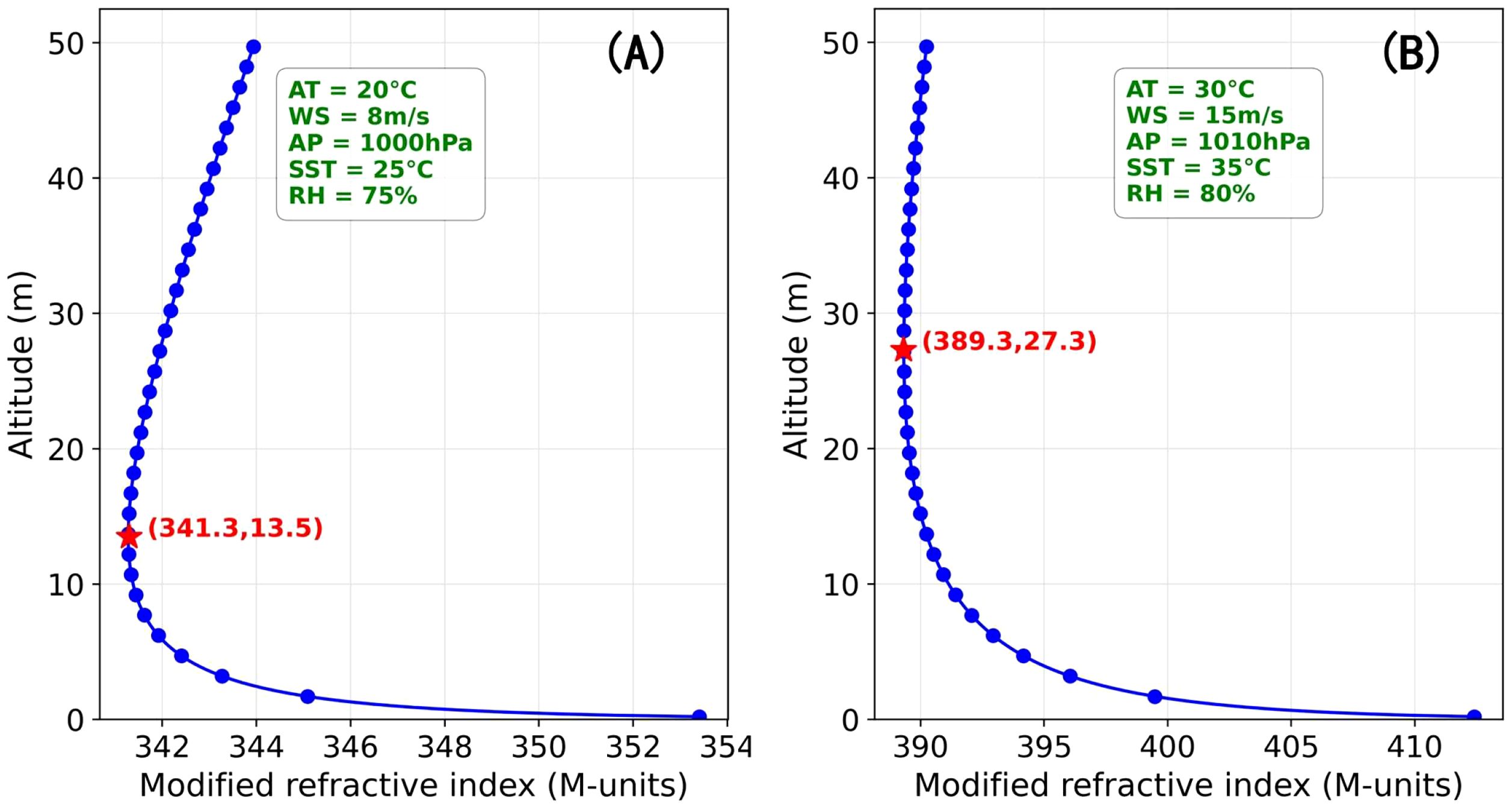
Figure 1. The M-profiles for EDHs of (a) 13.5m and (b) 27.3m, respectively.

2.4 Pierson-Moskowitz wave spectrum

The sea wave spectrum (Guerin and Johnson, 2015) mathematically characterizes the energy distribution of sea surface undulations across frequency and direction domains. This spectral representation quantifies the variance of sea surface displacement as a spectral density function in wavenumber space (spatial frequency domain). Through Fourier transformation, it decomposes stochastic sea surfaces into constituent wave components with distinct frequencies and propagation directions. In practical applications, the 2D ocean wave spectrum is typically expressed as the product of a directional spreading function $D(k)$ and a wavenumber spectrum $S(k)$, as shown in Equation 35:

$\begin{array}{ll}S(\mathbf{\text{k}})=\frac{1}{k}S(k)D(k)& (35)\end{array}$

where $\mathbf{\text{k}}=(k_x,k_y)$ constitutes a wavenumber vector. The wavenumber $k=\parallel \mathbf{\text{k}}\parallel =\sqrt{k_x^2+k_y^2}$ quantifies spatial wave frequency, defined as the number of complete wave cycles per unit length. The PM spectrum (Pierson and Moskowitz, 1964), empirically derived from 1964 North Atlantic wave measurements, serves as the canonical model for energy distribution in fully-developed seas under constant wind forcing. This spectral formulation establishes quantitative relationships between wave energy density and spectral components in equilibrium wind-wave systems. For modeling surface waves, the equation of the PM spectrum is defined as Equation 36:

$\begin{array}{ll}{S}_{PM}(k)=\frac{\alpha }{2k^3}·\exp (-\frac{\beta g^2}{k^2{U}_{19.5}^4})& (36)\end{array}$

where $\alpha$=0.0081 and $\beta$=0.74 are dimensionless constants, g denotes gravitational acceleration, and $U_{19.5}$ denotes the WS value at an elevation of 19.5 m above the sea surface.

After obtaining the PM spectral density, a Monte Carlo methodology can be used to simulate 2D rough sea surfaces (Meng et al., 2024). This method models the sea surface as a superposition of stochastic-amplitude harmonic components with stochastic amplitudes following independent Gaussian distributions. In the frequency domain, Gaussian white noise is filtered through a PM spectral model incorporating wind-wave dynamics, which imposes wave number-dependent energy constraints. An inverse Fourier transform then converts these filtered spectral components into spatially correlated sea surface height fluctuations that statistically match the target PM spectrum. For a 2D random rough surface with spatial dimensions $L_x=M·\text{Δ}x$ and $L_y=N·\text{Δ}y$, where M and N denote the number of grid points along the x- and y-axes, respectively, $\text{Δ}x$ and $\text{Δ}y$ represent the grid resolutions, the height $f(x_m,y_n)$ at each surface coordinate ($x_m=m\text{Δ}x$, $y_n=n\text{Δ}y$) can be formulated as Equation 37:

$\begin{array}{ll}f(x_m,y_n)=\frac{1}{L_x{L}_y}{\displaystyle \sum _{m_k=-M/2+1}^{M/2}{\displaystyle \sum _{n_k=-N/2+1}^{N/2}F(k_{m_k},k_{n_k})}}·\exp [i(k_{m_k}{x}_m+k_{n_k}{y}_n)]& (37)\end{array}$

The Fourier transform of the discrete function is denoted as $F(k_{m_k},k_{n_k})$, where $k_m$ and $k_n$ denote the spatial frequency components along the x- and y-axes. Its explicit mathematical form is defined by Equation 38:

$\begin{array}{ll}F(k_{m_k},k_{n_k})=2\pi {[L_x{L}_{y}S(k_{m_k},k_{n_k})]}^{1/2}·\{\begin{array}{cc}\frac{[N(0,1)+iN(0,1)]}{\sqrt{2}},& m_k\ne 0,M/2, and{n}_k\ne 0,N/2\\ N(0,1),& m_k\ne 0,M/2, and{n}_k\ne 0,N/2\end{array}& (38)\end{array}$

Figure 2 presents PM spectral model-generated 2D sea surface profiles under varying WSs (3–10 m/s). Analysis shows a strong correlation between wind forcing and sea surface dynamics: lower wind velocities produce mild surface undulations, while increased WSs trigger nonlinear height fluctuation amplification, reflecting enhanced wave-turbulence interactions.

Figure 2

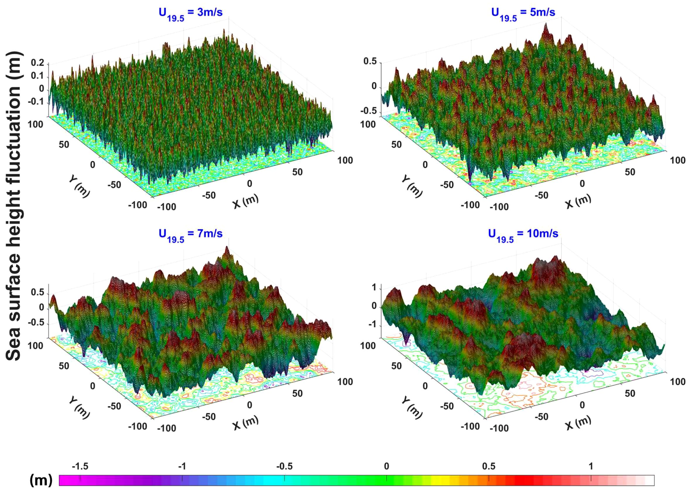
Figure 2. Rough sea surfaces generated using the PM spectrum under varying WS conditions.

3 Construction of spatially-varying evaporation duct refractivity field using meteorological reanalysis data

High-fidelity modeling of spatially-varying marine evaporation duct environments requires high-resolution meteorological parameter fields as fundamental inputs. Meteorological reanalysis data, particularly through their multiscale coupling and physically consistent boundary layer parameterization schemes, offer an effective technical approach for deriving accurate spatial distributions of meteorological elements (Ji et al., 2024a). ERA5 (Ji et al., 2024b), the fifth-generation global atmospheric reanalysis dataset published by the European Centre for Medium-Range Weather Forecasts, employs an advanced data assimilation framework that synergizes multi-source observations (satellite retrievals, surface stations, radiosondes) with numerical weather models. This integration generates spatiotemporally continuous meteorological fields with enhanced fidelity compared to its predecessor ERA-Interim (Yang et al., 2022a).

The South China Sea (SCS, 4°N–23°N, 105°E–118°E), a semi-enclosed tropical marginal sea influenced by complex atmospheric dynamics, maintains year-round high temperatures and humidity due to the interplay of meteorological and topographical factors. Using ERA5 reanalysis data, we extract six key meteorological parameters for evaporation duct modeling: AT, AP, zonal/meridional wind velocities, dewpoint temperature (DT), and SST. Table 1 details these parameters with their corresponding vertical levels. Figure 3 illustrates their spatial distribution across the SCS on March 1, 2025 at 00:00 UTC, revealing significant spatial heterogeneity in all meteorological parameters between different geographic locations.

Table 1

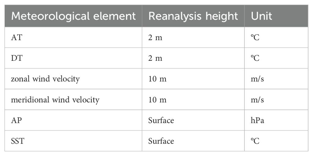
Table 1. Retrieved parameters along with corresponding reanalysis height levels.

Figure 3

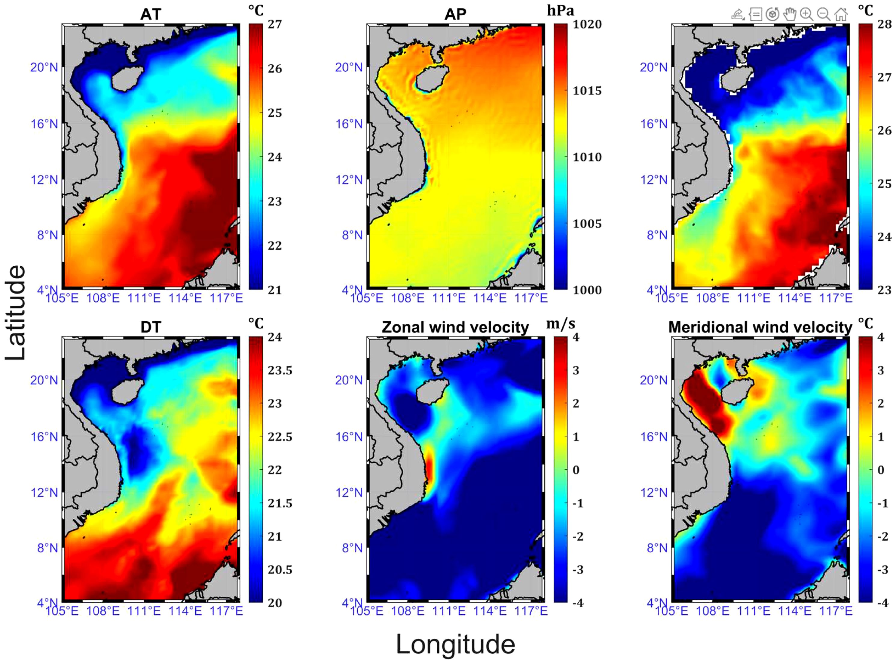
Figure 3. Spatial distribution of meteorological parameters in the SCS.

The WS is calculated by vectorially summing the zonal and meridional wind velocities, as shown in Equation 39:

$\begin{array}{ll}WS=\sqrt{u^2+v^2}& (39)\end{array}$

where u and v denote the zonal and meridional wind velocity components, respectively. RH is calculated using the Magnus-Tetens approximation (Alduchov and Eskridge, 1996), which employs AT and DT to determine saturation vapor pressure (Lawrence, 2005), as shown in Equations 40-42:

$\begin{array}{ll}{e}_s(T)=6.112·\exp \left(\frac{17.62·T}{T+243.12}\right)& (40)\end{array}$

$\begin{array}{ll}e(T_d)=6.112·\exp \left(\frac{17.62·T_d}{T_d+243.12}\right)& (41)\end{array}$

$\begin{array}{ll}RH=\frac{e(T_d)}{e_s(T)}\times 100\%& (42)\end{array}$

where T and $T_d$ denote AT and DT in degrees Celsius, respectively. This study incorporates derived WS and RH parameters along with AT, AP, and SST into the NPS model to simulate evaporation ducts.

Figure 4 illustrates the spatial distribution of evaporation duct refractivity calculated using the NPS model with reanalysis meteorological data from Figure 3. The projection of the study area onto longitude-latitude coordinates is simultaneously displayed. Significant spatial heterogeneity in refractivity is observed due to variations in meteorological parameters across geographic locations. For this investigation, we select an EM emission source at 111°E, 19.75°N. This location was explicitly configured as the radiation origin with EM wave propagation azimuthally fixed at 90° (true east). We focus on the evaporation duct along this eastern bearing where spatial refractivity heterogeneity is identified. Subsequent phases will implement numerical modeling of ducting effects along this bearing, with specific focus on quantifying PL anomalies under non-standard atmospheric conditions.

Figure 4

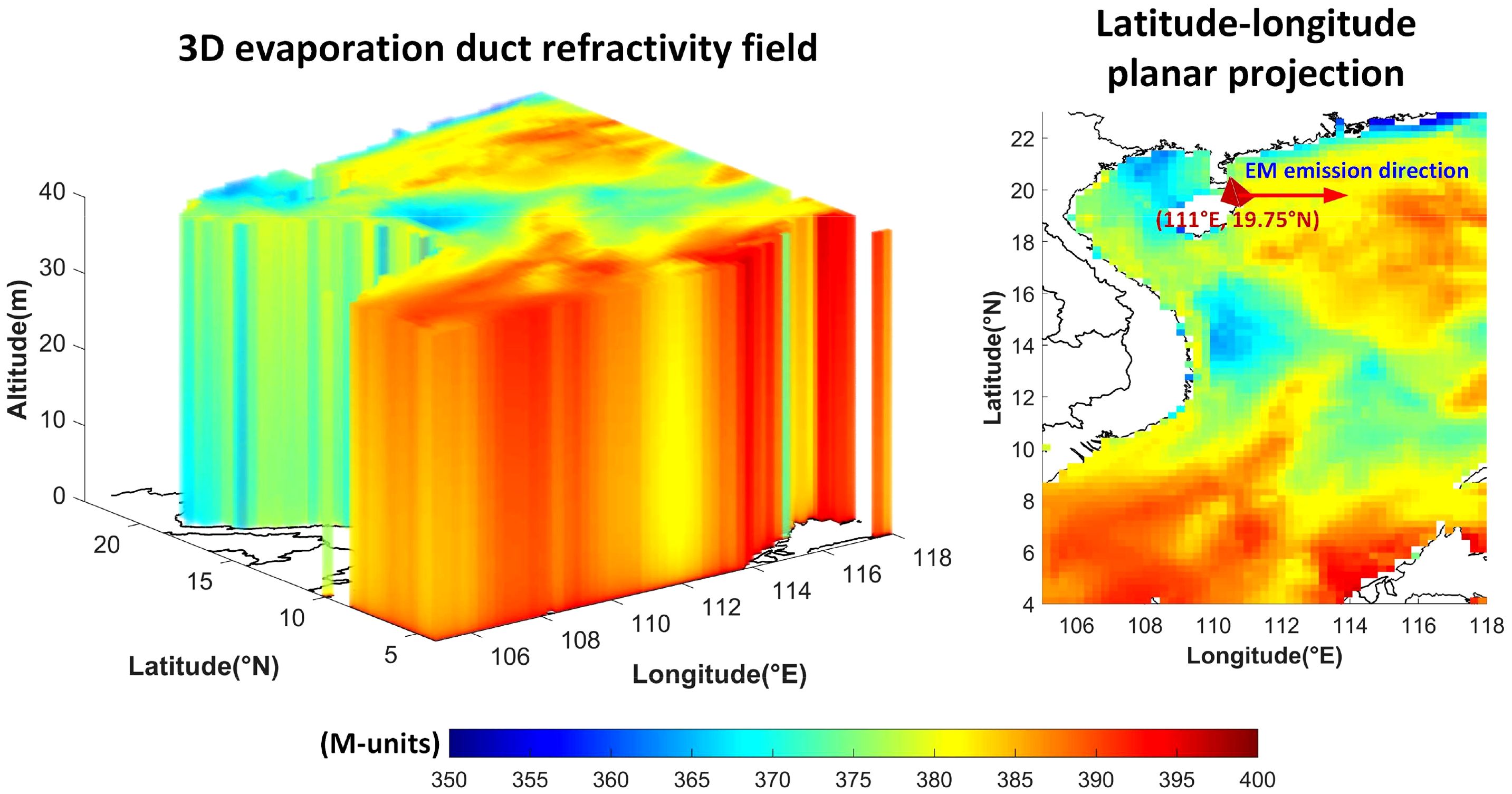
Figure 4. 3D evaporation duct refractivity field and its horizontal projection in longitude-latitude plane.

4 Computational modeling of EM propagation in evaporation duct environments

We perform EM wave PL simulations using a 3DPE framework, incorporating both the computed 3D refractivity field (constructed along the EM emission direction) and a numerically generated rough sea surface under 10 m/s WS condition. Beyond spatially-varying ducts, we simulate 3D PL characteristics under both standard atmospheric conditions and uniform evaporation duct environments, where the latter employs the refractive index profile shown in Figure 1. The simulation framework incorporates a radar system operating at 10 GHz with the following configuration: antenna altitude of 5 m, horizontal polarization, elevation angle of 0°, and azimuthal half-power beamwidth of 15°.

Numerical simulations model EM wave propagation over smooth sea surfaces (Figure 5), revealing distinct characteristics between standard atmospheric and evaporation duct environments. Under conventional atmospheric refraction (Figure 5A), EM attenuation stems primarily from free-space spreading and medium absorption, showing exponential signal decay with distance. In contrast, evaporation ducts create vertically stratified refractive gradients that enable anomalous propagation. This ducting effect confines EM energy within the atmospheric layer, reducing dielectric losses and permitting OTH signal transmission with non-exponential attenuation patterns. While standard environments cause rapid signal divergence, duct propagation preserves signal integrity beyond standard refractive limits, though partial energy leakage still occurs at duct boundaries. As EDH increases (Figures 5B, C), the duct structure’s EM wave trapping capability intensifies. Elevated EDH configurations demonstrate enhanced confinement of EM waves, enabling lower-loss propagation with extended transmission distances. This improved confinement mechanism allows sustained wave guidance while significantly reducing energy dissipation over extended propagation paths.

Figure 5

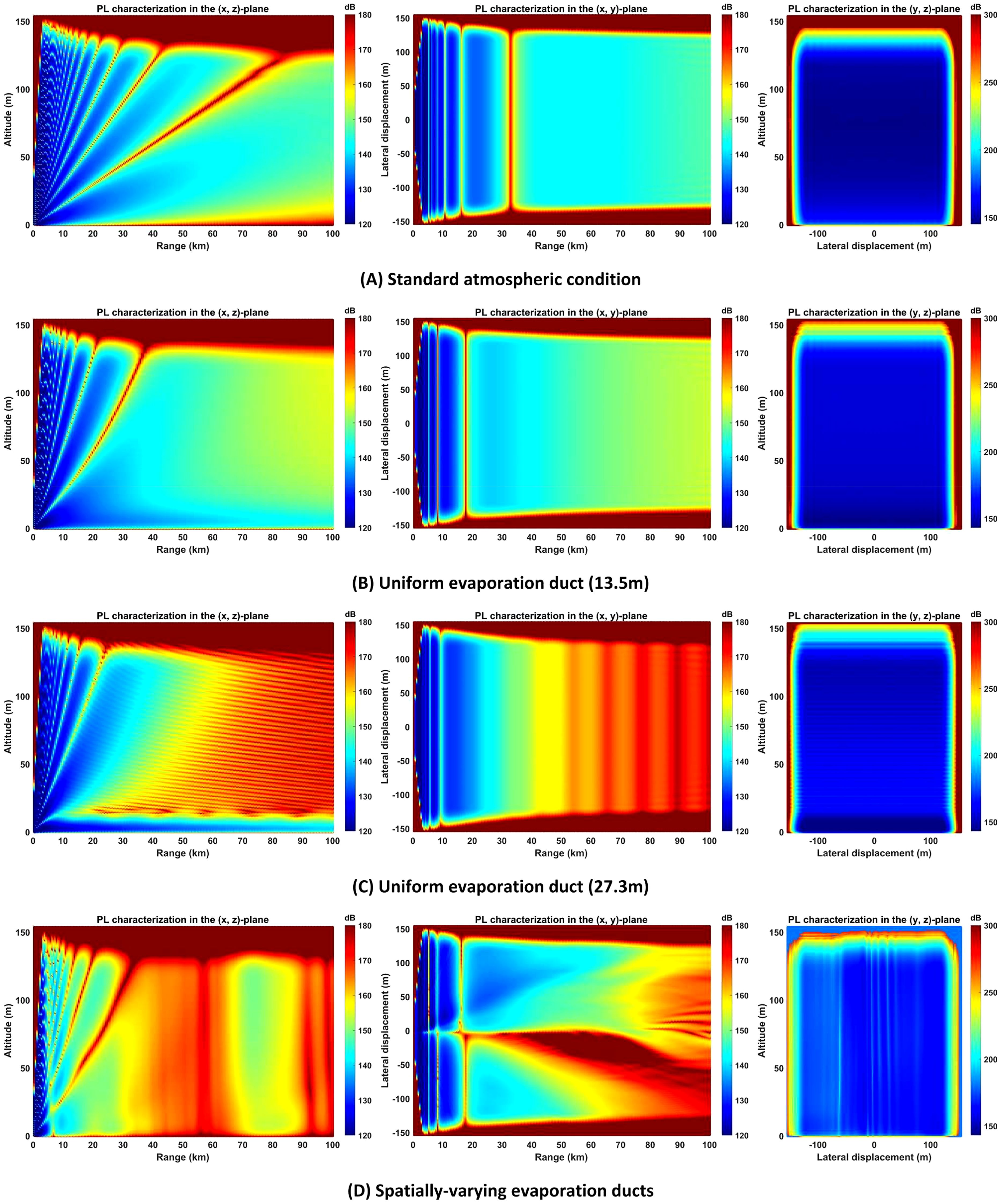
Figure 5. 3D PL characterization over smooth sea surfaces in: (A) standard atmosphere, (B) uniform evaporation duct with 13.5m EDH, (C) uniform evaporation duct with 27.3m EDH, and (D) spatially-varying evaporation duct environments.

The propagation characteristics in spatially-varying duct media (Figure 5D) demonstrate fundamentally distinct behaviors compared to those within homogeneous evaporation ducts. This divergence primarily stems from the inherent structural inhomogeneity of the medium, which induces multiscale interactions including localized reflection, refraction, and scattering phenomena. The presence of spatially varying refractive index profiles across different regions causes alterations in phase velocity and ray path divergence during propagation. Such refractive index gradients generate complex interference patterns through multipath propagation mechanisms, thereby introducing heightened complexity in predicting signal propagation trajectories and energy distribution characteristics. These anisotropic propagation effects significantly deviate from the deterministic path confinement observed in uniform ducting structures.

Experimental observations demonstrate that EM wave propagation over rough sea surfaces produces striped shadow patterns in PL field distributions (Figure 6). Compared to smooth sea conditions, rough sea surfaces exhibit accelerated attenuation rates and expanded blind zones due to surface roughness effects. This phenomenon primarily results from wave crest-induced shadow effects, which amplify multipath interference through enhanced reflection, scattering, and attenuation processes. Significant PL intensification occurs under conditions of pronounced sea surface height variations and active wave motion, substantially compromising transmission reliability.

Figure 6

Figure 6. 3D PL characterization over rough sea surfaces in: (A) standard atmosphere, (B) uniform evaporation duct with 13.5m EDH, (C) uniform evaporation duct with 27.3m EDH, and (D) spatially-varying evaporation duct environments.

5 Empirical PL observation-based performance validation of 3DPE framework

The China Research Institute of Radiowave Propagation (CRIRP) executed an EM wave OTH propagation observation in the SCS (Figure 7), using the research vessel Qiongsha 3, equipped with an S-band radar system (Ji et al., 2024b). Key system parameters are summarized in Table 2. During the 15-hour maritime campaign between Wenchang City (19°33’N, 110°49’E) and Yongxing Island (16°84’N, 112°33’E) as shown in Figure 7, the mobile platform transmitted S-band radar signals while shore-based stations along Hainan coast continuously received OTH signals. The coastal reception system incorporated a low-noise amplifier (LNA) in its front-end circuitry to optimize signal-to-noise ratio during prolonged monitoring. The EM PL is quantified by rigorously applying radar equations to OTH signals received during experimental configurations (Guo et al., 2019), as shown in Equation 43:

Figure 7

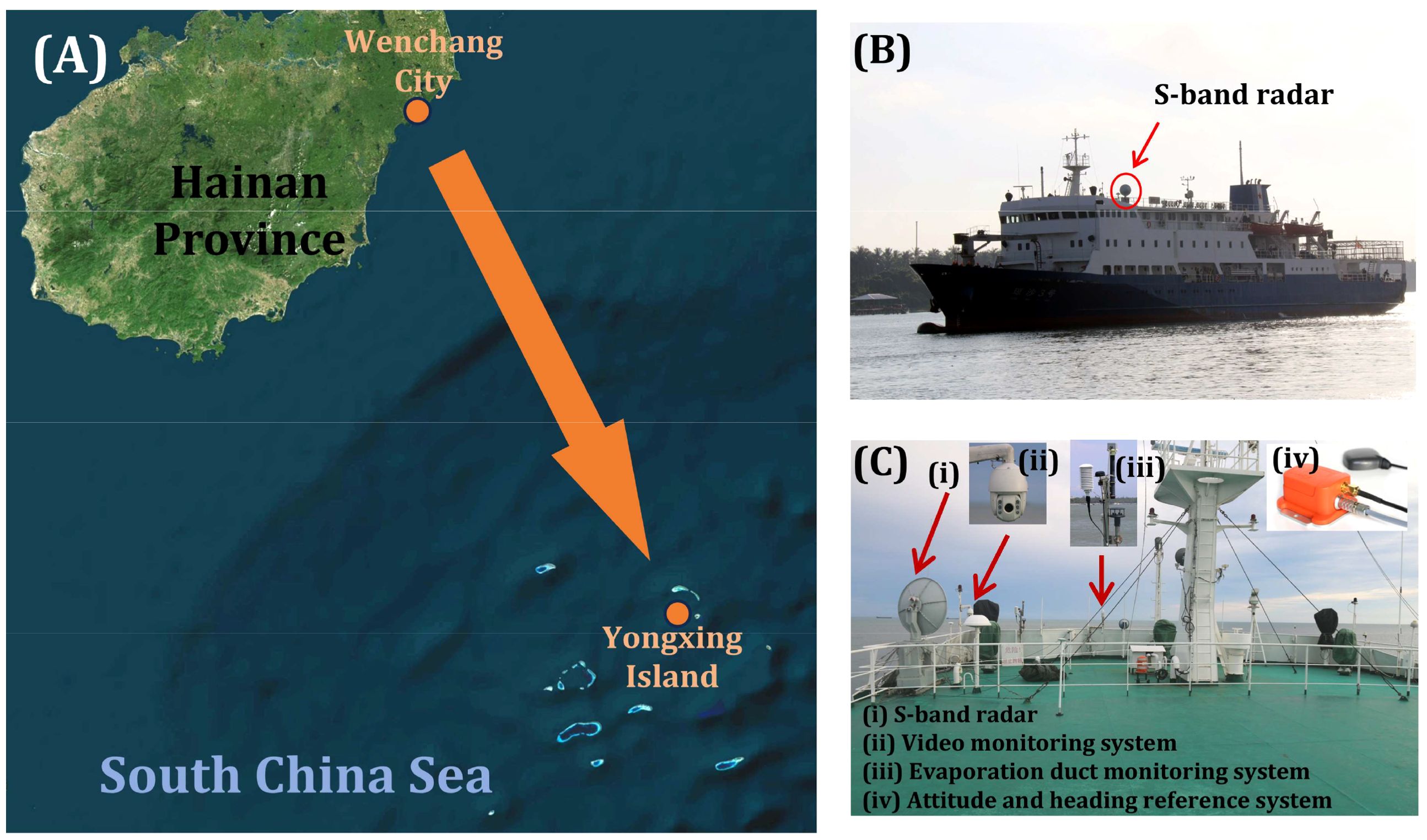
Figure 7. EM wave OTH propagation observation campaign: (A) vessel navigation trajectory, (B) Qiongsha 3 research vessel, (C) S-band radar system and auxiliary experimental instruments.

Table 2

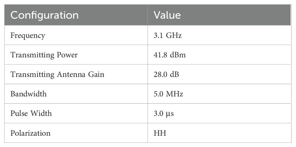
Table 2. Primary operational parameters.

$\begin{array}{ll}{L}_{obs}=P_t+G_t+G_r+G_{LNA}-P_r-L_t-L_r& (43)\end{array}$

where $P_t$ and $P_r$ denote the transmit power and received power, respectively; $G_t$ and $G_r$represent the antenna gains at the transmitter and receiver ends, respectively; while $L_t$ and $L_r$indicate the feeder line losses at the transmitter and receiver sides, respectively.

During the Qiongsha 3 research vessel’s transect from Wenchang City to Yongxing Island, we deployed a multi-sensor evaporation duct monitoring system (EDMS) to collect high-resolution meteorological and oceanographic data (Zhang et al., 2020). This integrated system incorporated meteorological sensors and infrared SST radiometers, continuously measuring five key variables—including AT, RH, WS, AP, and SST. Following data acquisition, parameters underwent preprocessing for outlier removal and temporal alignment before being fed into the NPS model to generate modified refractivity profiles (Ji et al., 2024c). This methodology enabled quantitative characterization of spatially heterogeneous evaporation duct structures.

To rigorously validate the 3DE framework’s efficacy and precision, we conduct systematic verification experiments using the 2DPE propagation model. Shipborne meteorological parameters are processed to generate non-uniform refractive index profiles and integrated into both computational frameworks, ensuring atmospheric condition consistency. Validation strictly followed Table 2 parameters, with results compared against the 3DPE model implementation. The 2DPE model configuration utilizes a Gaussian antenna profile for initial field distribution calculation to accurately simulate practical EM emission scenarios. This implementation employs a 2D window function for upper boundary processing, while enhancing lower boundary conditions through a roughness attenuation factor that modifies Fresnel reflection coefficients at impedance surfaces. The Miller-Brown (Guo et al., 2023) formulation is adopted to quantify surface roughness characteristics.

The comparative analysis reveals distinct morphological differences between measured and simulated PL characteristics (Figure 8). Field observations exhibit stochastic nonlinear fluctuations attributable to complex marine environmental factors, whereas parabolic equation method simulations under idealized assumptions generate smoothed attenuation curves. This constitutes the primary source of discrepancy between measured and simulated PLs. The established 3DPE framework demonstrates superior alignment with experimental data, accurately reproducing both the attenuation trend and numerical magnitudes. In contrast, 2DPE calculations show significant deviations in magnitude and fail to capture observed attenuation patterns, with discrepancies amplifying with transmission range. These findings empirically validate the 3DPE framework’s enhanced capability in modeling EM wave propagation within complex environments featuring anisotropic refractivity gradients and rough sea surface boundaries. In contrast, the 2DPE methodology employs simplified environmental assumptions (Zhang et al., 2021).

Figure 8

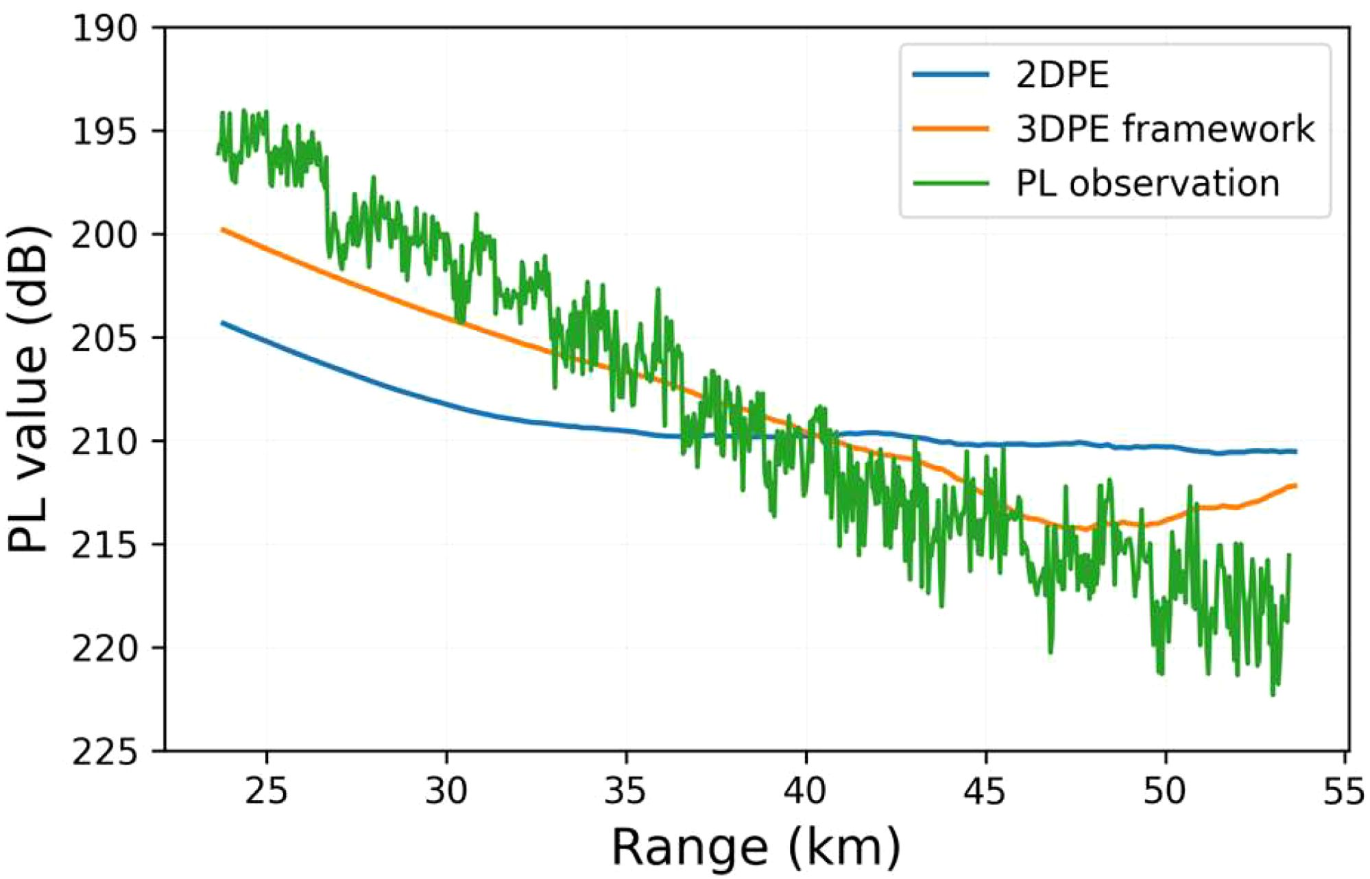
Figure 8. Comparison of PL values calculated by 3DPE framework and 2DPE with actual observation.

We quantitatively compare PL observations with two simulation results using three statistical metrics: root mean square error (RMSE), mean absolute error (MAE), and mean absolute percentage error (MAPE). These metrics provide multidimensional accuracy assessment: RMSE highlights larger deviations by squaring errors, MAE measures average error magnitude linearly, while MAPE calculates relative error percentages unaffected by absolute values. The corresponding formulas are defined as Equations 44–46. Quantitative evaluation demonstrates notable differences in prediction accuracy between the models. The 2DPE model shows significant PL prediction errors with metrics of 6.173 dB (RMSE), 5.424 dB (MAE), and 2.617% (MAPE). In comparison, the 3DPE model achieves substantially improved performance under identical test conditions, yielding 3.450 dB RMSE, 2.821 dB MAE, and 1.355% MAPE. Through comprehensive metric analysis, the 3DPE framework demonstrates significant advantages over traditional 2DPE method. Specifically, it achieves performance improvements of 54.301%, 47.990%, and 48.223% in RMSE, MAE, and MAPE respectively, with an overall error reduction exceeding 40%–quantitatively confirming the superiority of 3D EM modeling in complex propulsion system analysis.

$\begin{array}{ll}RMSE=\sqrt{\frac{1}{n}{\displaystyle \sum _{i=1}^n{(L_{obs}^{(i)}-L_s^{(i)})}^2}}& (44)\end{array}$

$\begin{array}{ll}MAE=\frac{1}{n}{\displaystyle \sum _{i=1}^n|L_{obs}^{(i)}-L_s^{(i)}|}& (45)\end{array}$

$\begin{array}{ll}MAPE=\frac{100\%}{n}{\displaystyle \sum _{i=1}^n|}\frac{L_s^{(i)}-L_{obs}^{(i)}}{L_{obs}^{(i)}}|& (46)\end{array}$

where $L_s$ denotes simulated PL, n specifies the number of observational samples.

6 Conclusion

This study examines EM wave propagation through spatially-varying evaporation ducts above rough sea surfaces, focusing on addressing limitations of conventional 2D modeling approaches. Traditional 2D models impose restrictive homogeneity assumptions within propagation planes, failing to account for critical refractive index variations characteristic of real maritime environments. Our analysis reveals that the 2DPE model shows significant prediction errors in PL estimation, with RMSE, MAE, and MAPE attaining 6.173dB, 5.424dB, and 2.617% respectively. In contrast, the 3DPE model demonstrates substantially improved accuracy under identical conditions, achieving 3.450dB (RMSE), 2.821dB (MAE), and 1.355% (MAPE). This represents an overall error reduction exceeding 40% compared to the 2D baseline, conclusively validating 3D modeling’s superior capability in handling complex wave propagation phenomena. These advancements establish new capabilities for precise EM environmental characterization, paving the way for enhanced maritime communication systems.

Data availability statement

The original contributions presented in the study are included in the article/supplementary material. Further inquiries can be directed to the corresponding authors.

Author contributions

HJ: Funding acquisition, Writing – original draft. LG: Funding acquisition, Writing – original draft, Project administration, Conceptualization, Supervision. YZ: Software, Writing – original draft, Resources. TN: Writing – review & editing, Software. YW: Writing – review & editing, Funding acquisition. JZ: Writing – review & editing, Funding acquisition, Validation, Project administration. QL: Writing – review & editing, Formal Analysis. XG: Writing – review & editing, Investigation. YSZ: Writing – review & editing, Data curation.

Funding

The author(s) declare that financial support was received for the research and/or publication of this article. This work was supported in part by the National Natural Science Foundation of China under Grant U21A20457, Grant 62231021, Grant 62371380, and Grant 62271457; and in part by the Stabled-Support Scientific Project of China Research Institute of Radiowave Propagation under Grant A132301214; and in part by the Fundamental Research Funds for the Central Universities under Grant YJSJ25020; and in part by the Innovation Fund of Xidian University.

Conflict of interest

The authors declare that the research was conducted in the absence of any commercial or financial relationships that could be construed as a potential conflict of interest.

Generative AI statement

The author(s) declare that no Generative AI was used in the creation of this manuscript.

Publisher’s note

All claims expressed in this article are solely those of the authors and do not necessarily represent those of their affiliated organizations, or those of the publisher, the editors and the reviewers. Any product that may be evaluated in this article, or claim that may be made by its manufacturer, is not guaranteed or endorsed by the publisher.

References

Alduchov O. A. and Eskridge R. E. (1996). Improved Magnus form approximation of saturation vapor pressure. J. Appl. Meteorol. 35, 601–609. doi: 10.1175/1520-0450(1996)035<0601:IMFAOS>2.0.CO;2

Crossref Full Text | Google Scholar

Anderson K. D. (1995). Radar detection of low-altitude targets in a maritime environment. IEEE Trans. Antennas Propag. 43, 609–613. doi: 10.1109/8.387177

Crossref Full Text | Google Scholar

Babin S. M. and Dockery G. D. (2002). LKB-Based evaporation duct model comparison with buoy data. J. Appl. Meteorol. 41, 434–446. doi: 10.1175/1520-0450(2002)041<0434:LBEDMC>2.0.CO;2

Crossref Full Text | Google Scholar

Babin S. M., Young G. S., and Carton J. A. (1997). A new model of the oceanic evaporation duct. J. Appl. Meteorol. 36, 193–204. doi: 10.1175/1520-0450(1997)036<0193:ANMOTO>2.0.CO;2

Crossref Full Text | Google Scholar

Barrios A. (1994). A terrain parabolic equation model for propagation in the troposphere. IEEE Trans. Antennas Propag. 42, 90–98. doi: 10.1109/8.272306

Crossref Full Text | Google Scholar

Douchin N., Bolioli S., Christophe F., and Combes P. (1994). Theoretical study of the evaporation duct effects on satellite-to-ship radio links near the horizon. IEE Proc. - Microwaves Antennas Propagation 141, 272–278. doi: 10.1049/ip-map:19941168

Crossref Full Text | Google Scholar

Fabbro V., Bourlier C., and Combes P. F. (2006). Forward propagation modeling above gaussian rough surfaces by the parabolic shadowing effect. Prog. Electromagnetics Res. 58, 243–269. doi: 10.2528/PIER05090101

Crossref Full Text | Google Scholar

Fairall C. W., Bradley E. F., Hare J. E., Grachev A. A., and Edson J. B. (2003). Bulk parameterization of air-sea fluxes: Updates and verification for the COARE algorithm. J. Clim. 16, 571–591. doi: 10.1175/1520-0442(2003)016(0571:BPOASF)2.0.CO;2

Crossref Full Text | Google Scholar

Fairall C. W., Bradley E. F., Rogers D. P., Edson J. B., and Young G. S. (1996). Bulk parameterization of air-sea fluxes for Tropical Ocean-Global Atmosphere Coupled-Ocean Atmosphere Response Experiment. J. Geophys. Res. 101, 3747–3764. doi: 10.1029/95JC03205

Crossref Full Text | Google Scholar

Feit M. D. and Fleck J. A. (1978). Light propagation in graded-index optical fibers. Appl. Optics. 17, 3990–3998. doi: 10.1364/AO.17.003990

PubMed Abstract | Crossref Full Text | Google Scholar

Grachev A. A., Andreas E. L., Fairall C. W., Guest P. S., and Persson P. O. G. (2007). SHEBA flux-profile relationships in the stable atmospheric boundary layer. Bound.-Layer Meteor. 124, 315–333. doi: 10.1007/s10546-007-9177-6

Crossref Full Text | Google Scholar

Grachev A. A. and Fairall C. W. (1997). Dependence of the Monin-Obukhov stability parameter on the bulk Richardson number over the ocean. J. Appl. Meteor. 36, 406–414. doi: 10.1175/1520-0450(1997)036<0406:DOTMOS>2.0.CO;2

Crossref Full Text | Google Scholar

Guerin C. and Johnson J. T. (2015). A simplified formulation for rough surface cross-polarized backscattering under the second-order small-slope approximation. IEEE Trans. Geosci. Remote Sensing. 53, 6308–6314. doi: 10.1109/TGRS.2015.2440443

Crossref Full Text | Google Scholar

Guo X., Li Q., Zhao Q., Kang S., Wei Y., and Yang L. (2023). A comparative study of rough sea surface and evaporation duct models on radio wave propagation. IEEE Trans. Antennas Propag. 71, 6060–6071. doi: 10.1109/TAP.2023.3276571

Crossref Full Text | Google Scholar

Guo X., Zhao D., Zhang L., Wang H., Kang S., and Lin L. (2019). C band transhorizon signal characterisations in evaporation duct propagation environment over Bohai Sea of China. IET Microwaves Antennas Propagation 13, 407–413. doi: 10.1049/iet-map.2018.5040

Crossref Full Text | Google Scholar

Hardin R. H. and Tappert F. D. (1973). Applications of the split-step Fourier method to the numerical solution of nonlinear and variable coefficient wave equations. SIAM Rev. 15, 423.

Google Scholar

Harrington R. F. (2001). Time-harmonic electromagnetic fields (John Wiley & Sons).

Google Scholar

Hitney H. V., Richter J. H., Pappert R. A., Anderson K. D., and Baumgartner G. B. (1985). Tropospheric radio propagation assessment. Proc. IEEE. Wiley-IEEE Press 73, 265–283. doi: 10.1109/PROC.1985.13138

Crossref Full Text | Google Scholar

Hu H., Chai S., and Mao J. (2005). “Field strength prediction behind a lossy dielectric block by using the 3D parabolic equation model,” in 2005 Asia-Pacific Microwave Conference Proceedings. (Suzhou, China: IEEE) 1–4. doi: 10.1109/APMC.2005.1606416

Crossref Full Text | Google Scholar

Janaswamy R. (2001). Radio wave propagation over a nonconstant immittance plane. Radio Sci. 36, 387–405. doi: 10.1029/2000RS002338

Crossref Full Text | Google Scholar

Janaswamy R. (2003). Path loss predictions in the presence of buildings on flat terrain: a 3-D vector parabolic equation approach. IEEE Trans. Antennas Propag. 51, 1716–1728. doi: 10.1109/TAP.2003.815415

Crossref Full Text | Google Scholar

Ji H., Guo L., Zhang J., Wei Y., Guo X., and Zhang Y. (2024a). EDH-STNet: An evaporation duct height spatiotemporal prediction model based on Swin-Unet integrating multiple environmental information sources. Remote Sens. 16, 4227. doi: 10.3390/rs16224227

Crossref Full Text | Google Scholar

Ji H., Guo L., Zhang J., Wei Y., Guo X., Zhang Y., et al. (2024b). IPILT–OHPL: An over-the-horizon propagation loss prediction model established by incorporating prior information into the LSTM–Transformer structure. IEEE J. Sel. Top. Appl. Earth Observ. Remote Sens. 17, 10067–10082. doi: 10.1109/JSTARS.2024.3395630

Crossref Full Text | Google Scholar

Ji H., Wei Y., Zhao Q., Guo L., and Zhang J. (2024c). EKDInformer-LTEDH: an Informer-based environmental knowledge-driven prediction model for long-term evaporation duct height. IEEE Geosci. Remote Sens. Lett. 21, 1–5. doi: 10.1109/LGRS.2024.3468290

Crossref Full Text | Google Scholar

Kuttler J. R. and Janaswamy R. (2002). Improved Fourier transform methods for solving the parabolic wave equation. Radio Sci. 37, 1–5. doi: 10.1029/2001RS002488

Crossref Full Text | Google Scholar

Lawrence M. G. (2005). The relationship between relative humidity and the dewpoint temperature in moist air: A simple conversion and applications. Bull. Amer. Meteorol. Soc 86, 225–233. doi: 10.1175/BAMS-86-2-225

Crossref Full Text | Google Scholar

Levy M. (2000). Parabolic equation methods for electromagnetic wave propagation (IET Digital Library: IEE Electromagnetic Wave Series).

Google Scholar

Meng X., Su J., Li K., Dong C., Hou G., Liu Y., et al. (2024). An effective composite scattering model for the sea surface with a target based on the TSBR-TSM algorithm. IEEE Antennas Wirel. Propag. Lett. 23, 2411–2415. doi: 10.1109/LAWP.2024.3393773

Crossref Full Text | Google Scholar

Paulus R. A. (1985). Practical application of an evaporation duct model. Radio Sci. 20, 887–896. doi: 10.1029/RS020i004p00887

Crossref Full Text | Google Scholar

Pierson W. J. and Moskowitz L. (1964). A proposed spectral form for fully developed wind seas based on the similarity theory of S. A. Kitaigorodskii. J. Geophys. Res. 69, 5181–5190. doi: 10.1029/JZ069i024p05181

Crossref Full Text | Google Scholar

Ray A., Ray M., and Basuray A. (2019). Plane wave spectrum analysis of transverse discontinuities in dielectric waveguide I. Reflection coefficients. Opt. Eng. 58, 117103. doi: 10.1117/1.OE.58.11.117103

Crossref Full Text | Google Scholar

Thomson A. D. and Quach T. D. (2005). Application of parabolic equation methods to HF propagation in an Arctic environment. IEEE Trans. Antennas Propag. 53, 412–419. doi: 10.1109/TAP.2004.838751

Crossref Full Text | Google Scholar

Wang S., Yang K., Shi Y., Yang F., Zhang H., and Ma Y. (2023a). Prediction of over-the-horizon electromagnetic wave propagation in evaporation ducts based on the gated recurrent unit network model. IEEE Trans. Antennas Propag. 71, 3485–3496. doi: 10.1109/TAP.2023.3240998

Crossref Full Text | Google Scholar

Wang S., Yang K., Shi Y., Zhang H., Yang F., Hu D., et al. (2023b). Long-term over-the-horizon microwave channel measurements and statistical analysis in evaporation ducts over the Yellow Sea. Front. Mar. Sci. 10. doi: 10.3389/fmars.2023.1077470

Crossref Full Text | Google Scholar

Yang C., Shi Y., Wang J., and Feng F. (2022a). Regional spatiotemporal statistical database of evaporation ducts over the South China Sea for future long-range radio application. IEEE J. Sel. Top. Appl. Earth Observ. Remote Sens. 15, 6432–6444. doi: 10.1109/JSTARS.2022.3197406

Crossref Full Text | Google Scholar

Yang C. and Wang J. (2022). The investigation of cooperation diversity for communication exploiting evaporation ducts in the South China Sea. IEEE Trans. Antennas Propag. 70, 8337–8347. doi: 10.1109/TAP.2022.3177509

Crossref Full Text | Google Scholar

Yang C., Wang J., and Ma J. (2022b). Exploration of X-band communication for maritime applications in the South China Sea. IEEE Antennas Wirel. Propag. Lett. 21, 481–485. doi: 10.1109/LAWP.2021.3136044

Crossref Full Text | Google Scholar

Yang F., Wang S., Yang K., Shu Y., and Shi Y. (2024). Marine high-speed over-the-horizon communications and channel sensing in evaporation ducts over the South China Sea. IEEE Antennas Wirel. Propag. Lett. 23, 2870–2874. doi: 10.1109/LAWP.2024.3411057

Crossref Full Text | Google Scholar

Zhang H., Li Q., Guo X., and Hou C. (2021). “Research on radio wave propagation prediction model using 3-D parabolic equation over rough sea surface,” in 2021 International Applied Computational Electromagnetics Society (ACES-China) Symposium. 1–4. doi: 10.23919/ACES-China52398.2021.9581721

Crossref Full Text | Google Scholar

Zhang J., Wu Z, Zhang Y, and Wang B. (2012). Evaporation duct retrieval using changes in radar sea clutter power versus receiving height. Prog. In Electromagnetics Res. 126, 555–571. doi: 10.2528/PIER11121307

Crossref Full Text | Google Scholar

Zhang J., Wu Z., Zhu Q., and Wang B. (2011). A four-parameter m-profile model for the evaporation duct estimation from radar clutter. Prog. In Electromagnetics Res. 114, 353–368. doi: 10.2528/PIER11012204

Crossref Full Text | Google Scholar

Zhang J., Zhang Y., Xu X., Li Q., and Wu J. (2020). Estimation of sea clutter inherent Doppler spectrum from shipborne S-band radar sea echo. Chin. Phys. B. 29, 68402. doi: 10.1088/1674-1056/ab888a

Crossref Full Text | Google Scholar

Zhao X., Huang J., and Gong S. (2009). Modeling on multi-eigenpath channel in marine atmospheric duct. Radio Sci. 44, 106–110. doi: 10.1029/2008RS003847

Crossref Full Text | Google Scholar

Zhao W., Zhao J., Li J., Zhao D., Huang L., Zhu J., et al. (2021). An evaporation duct height prediction model based on a long short-term memory neural network. IEEE Trans. Antennas Propag. 69, 7795–7804. doi: 10.1109/TAP.2021.3076478

Crossref Full Text | Google Scholar