Abstract
Migrating sand waves are widely developed on the outer continental shelf and upper slope of the northern South China Sea (SCS), at water depth ranging from 80 m to 250 m. Recent works reveal the critical role of internal solitary waves (ISWs) in sand wave migration in this area. However, the physical mechanism and mathematical modeling on ISW-induced sand wave migration still have deficiencies. This paper proposes hydrodynamic and seabed models utilizing the Massachusetts Institute of Technology General Circulation Model (MITgcm) and Biot’s theory to evaluate bed load transports, in which the ISW-induced internal-surface coupling response of seabed is particularly considered. Results and analysis indicate that ISWs can induce excess pore pressure (EPP) in the seabed, resulting in upward seepage force acting on the sediment particles, and thus reduce the critical incipient shear stress and promote the initiation and transport of sediment at seabed surface. The ISW-induced transient EPP rather than the accumulated EPP dominates the internal pore pressure response of seabed. The ISW-induced erosion depth can be twice the transient liquefaction depth at the uppermost seabed layer if seepage force is added to the sediment force equation. With the bottom shear stress outputted by MITgcm as the external driving forces, combining the internal-surface coupling response of seabed, the bed load transport rate is effectively calculated. This paper provides effective tools to evaluate ISWs-induced bed load transport and suggests an important role of ISWs in the migration of sand waves on the outer continental shelf and upper slope in the northern SCS. Further in-situ observations are still needed to calibrate and verify the present model.
1 Introduction
Submarine sand waves, which are widely present in coastal and offshore areas (Feng and Xia, 1993; Wang and Li, 1994), represent a specific type of sedimentary geomorphology that arises from the interaction between the seabed and hydrodynamic-associated currents. Most of the submarine sand waves are migrating parallel to the direction of the currents (Zhuang et al., 2004; Gao, 2009), like terrestrial sand dunes propelled by wind. Hydrodynamics exert important influence on submarine sand waves, inducing significant changes in their position, morphology, and sediment mechanical properties (Xia et al., 2009). Sand wave migration can change the physical and sedimentary environment, further facilitating the transportation of water, sediments, nutrients and pollutants (Alford et al., 2015). Furthermore, sand wave migration can induce seabed erosion and deposition, potentially resulting in the overhanging, burial, and destruction of cables and pipelines (Leckie et al., 2016), as well as the failure of offshore platforms (Nemeth et al., 2003).
The hydrodynamics factors contributing to the migration of sand waves include waves, tidal currents, typhoons, internal waves, etc. The migration of sand waves is mainly determined by means of field observation, theoretical frameworks, and mathematical modeling. Various equations are employed in theoretical models (Rubin and Hunter, 1982; Qian and Wan, 1983) to calculate critical incipient velocity of sediments, sediment transport rates (Bai et al., 2009; Blondeaux and Vittori, 2016), and sand migrating rates (Zhou et al., 2018). Migrating sand waves are widely distributed on the outer continental shelf and upper slope in the northern South China Sea (SCS) at water depths ranging from 80 m to 250 m (Wu et al., 2006). These sand waves exhibit wave heights between 0.3 m and 5.6 m and wavelengths from 5 m to 140 m, covering small-scale, medium-scale, large-scale and giant-scale sand waves (Zhang et al., 2017). Comparative analysis of repeated multibeam survey results indicate that the migration rate and migration direction of sand waves show remarkable spatial variability (Zhong et al., 2007; Lin et al., 2009; Zhou et al., 2018). Traditional hydrodynamic factors such as waves, tidal currents and typhoon have difficulties in explaining these sand wave migration patterns. Waves and tidal currents serve as the background hydrodynamics with long-term effects. Surface waves, with extreme wave heights not exceeding 40~60 m, have minimal impacts on the seabed at 80-250 m depths (Wu et al., 2006). In the meanwhile, observations have revealed that the average bottom tidal current velocity in the sand wave region in the northern SCS is less than 0.15 m/s (Qiu and Fang, 1999; Luan et al., 2010). This velocity is insufficient to trigger sand wave migration. The northern SCS is frequently impacted by typhoons and tropical storms. Numerical simulation based on Regional Ocean Modeling Scheme (ROMS) indicates that bottom current velocities reached the critical incipient current velocity for sand during Typhoon Fanbia (Zhou et al., 2018). However, the sand wave migration attributed to the typhoon accounted for only 26.36% of the annual migration volume (Zhou et al., 2018), making it difficult to explain large-scale sand wave migration outside the period of typhoon events. Research indicates that internal solitary waves (ISWs) play a significant role in driving sand wave migration in the northern SCS as one of the most developed regions for ISWs in the world (Cai, 2015). The crest lines of ISWs captured by Synthetic Aperture Radar (SAR) images (Reeder et al., 2011) and the distribution of regional sand waves (Geng et al., 2017) aligns closely with areas of concentrated ISWs activity in northern SCS. ISWs would be the possible energy source of sand wave migration when they propagate forward northwest to the upper continental slope and shelf. Field observations frequently captured the sudden strong bottom currents induced by ISWs (Zhou et al., 2013). These strong currents in the sand wave region in the northern SCS can initiate the sediment (Xia et al., 2009), demonstrating a closed relationship between the sand waves and ISWs (Luan et al., 2010). Laboratory simulations of the interaction between ISWs and sandy slopes (Cacchione and Drake, 1986; Zhou et al., 2013; Tian et al., 2021) and field observations of sand wave migration (Zhang et al., 2019; Miramontes et al., 2020) all show that the stress and current fields induced by ISWs are direct external driving forces for sand wave migration. As ISWs propagate across continental slopes and shelves, they dissipate energy and generate sudden strong currents. It enhances sediment resuspension and transport (Tian et al., 2024b), significantly promoting sand wave migration. The high occurrence frequency of ISWs in the northern SCS contributes to an additive impact on the amount of sand wave migration, effectively explaining the large annual migration distance. In addition, ISWs may exhibit either depression or elevation morphologies, which can explain the phenomenon of sand waves migrating along slopes landward or seaward. In summary, for the region of water depth ranging from 80 m to 250 m of the continental shelf and upper slope in the northern SCS, waves, tidal currents and typhoons have difficulties in explaining the well-aligned migration of sand waves. However, the well-developed ISWs have been continuously verified by observations to be an important hydrodynamics factors driving the sand waves migration.
The energy dissipation of ISWs in shallow waters can cause strong horizontal and vertical mixing of seawater, and change the stress field on the seabed surface. Field observations show that the depression ISWs generate significant negative pressure disturbances on the seabed (Miramontes et al., 2020; Yang et al., 2022; Xie et al., 2024). The pressure fluctuations, detected by seafloor pressure sensors, exhibit a strong correlation with the kinetic energy of high-frequency ISW wave packets (Thomas et al., 2016). Analytical solutions reveal that ISW-induced seabed responses are sensitive to the shear modulus and density profile of the overlying water column. In many cases, this sensitivity may lead to shear failure of the seabed (Tong et al., 2024). Like the surface gravity waves propagating at the air-water interface, ISWs have both horizontal and vertical effects on the seabed as well. The refraction of ISWs along continental slopes can significantly increase the seabed shear stress to a higher level. It can exceed the critical threshold for sediment incipient motion (Droghei et al., 2016), promoting the migration of sand waves. Furthermore, ISW-induced pressure disturbances can penetrate into the seabed and modify the stress field to a certain depth. For example, the impact depth of ISWs-generated excess pore pressure (EPP) is estimated to be approximately an order of magnitude smaller than the ISWs wavelength, potentially extending to several tens of meters (Tian et al., 2019). A coupling response between the seabed surface and internal under ISWs actions, that is, the upward seepage pressure gradient significantly reduces the effective self-weight of sediment particles, thus facilitating the sediment initiation (Tian et al., 2023) and double the amount of resuspension (Rivera Rosario et al., 2017) at the seabed surface. To further elucidate the interaction between ISWs and the seabed, scholars have applied Biot’s theory to quantify the ISW-induced pore pressure and shear stress (Williams and Jeng, 2007). The parametric method has also been employed to analyze seabed responses within a two-layer stratified fluid system. It reveals that ISWs can generate inverse pressure gradients at the front of elevation ISWs and at the rear of depression ones (Chen and Hsu, 2005). Consequently, as ISWs approach the seabed, their wave peaks disrupt the unconsolidated sediments, significantly enhancing sediment resuspension in shallow waters (about 200 m depth). The sand migration induced by ISWs is governed by the interaction between hydrodynamics and seabed. A comprehensive understanding of this interaction is essential for accurately characterizing the mechanisms and developing models to predict sand wave migrations in the northern SCS. However, current research remains limited in fully characterize the dynamic process. Further evaluation models are required for the sand wave migration on the continental shelf and upper slope in the northern SCS.
This paper uses the Massachusetts Institute of Technology General Circulation Model (MITgcm) and Biot’s equation to simulate the hydrodynamic and seabed response, respectively. Through these simulations, this paper investigates the coupling of ISWs-induced internal response of the seabed including pore pressure, seepage, as well as the surface response such as sediment incipient motion and sediment transport rate. The effectiveness of ISWs simulation and the coupling response of seabed are validated by comparing with observations of ISWs propagation. Our models provide the temporally and spatially stress field induced by ISWs on the seabed surface and describe the internal-surface coupling response process of seabed, further giving effective methods to calculate ISW-induced sand wave migration.
2 Models to simulate ISWs and seabed response
2.1 Numerical model to simulate ISWs
MITgcm is a non-hydrostatic ocean numerical model based on the finite volume method. It has capabilities of non-hydrostatic approximation calculations, allowing the model to simulate multi-scale physical motions in the ocean. It is widely employed to simulate the generation and propagation of ISWs in the northern SCS (Liang et al., 2019; Zeng et al., 2024; Ren et al., 2025). The equations that govern the evolution obtained by the laws of classical mechanics and thermodynamics as Equations 1–7:
where r is the vertical coordinate system; t is the time; is a unit vector in the vertical direction; is the velocity vector; is the horizontal component of velocity; is the pressure or geopotential; is the angular velocity of Earth’s rotation; is the potential temperature; S is salinity; is the buoyancy force; is the total derivative, and is the ‘grad’ operator, with operating in the horizontal and operating in the vertical; 、 、 、 are the sums of the dissipative and external forcing terms for velocity, potential temperature and salinity, respectively (see http://mitgcm.org).
2.2 Models to calculate excess pore pressure in the seabed
There are two types of wave-induced EPP, that is, the transient one and the accumulated one, which depends on the way that the pore pressure is generated (Zen et al., 1998). The ISWs-induced EPP in the seabed is calculated by the Biot’s consolidation theory.
2.2.1 Transient pore pressure
The sand seabed consists of a skeleton composed of sediment particles and fluids filling the pores of the skeleton. In this model, the seabed is assumed to be isotropic, linearly elastic, and has little deformation, the seepage between pores conforms to Darcy’s law. In keeping with the simplified two-dimensional section of ISWs, the transient pore pressure is also focused on the horizontal and vertical x-z two dimensional response. Referring to the wave-induced transient pore pressure response of the seabed (Jeng et al., 2007), the continuity equation of seepage of pore water is:
where x is the direction ISWs propagating; z is the depth (zero at the seabed surface and positive downward); , are the permeability coefficients in the x and z directions, respectively; p is the transient pore pressure; is the unit weight of pore water; n is the soil porosity; is the compressibility of pore water, which can be expressed as Equation 9:
where K is the elastic bulk modulus of the seawater, taken as ; is the degree of saturation of the soil; is the absolute pore pressure, which can be simplified to take the value of the initial hydrostatic pressure, namely where is the reference density of the water body. is the volumetric strain of soil which can be expressed as Equation 10:
where u and w are the displacements in x and z directions, respectively. The force governing equations are:
where G is the shear modulus of the soil; ν is the Poisson’s ratio. The above Equations 8, 11, 12 can be solved with boundary conditions. At the seabed surface, the pore pressure is equal to the ISW-induced pressure, the vertical effective stress and the bed shear stress is approximately zero. The boundary conditions at the seabed surface can be expressed as Equations 13, 14:
At an infinite depth in the seabed, both soil displacement and pore pressure are zero, as Equation 15:
2.2.2 Accumulated pore pressure
If our view concentrates on the vertical response of EPP profile at one point of seabed at a fixed water depth, the one-dimensional Biot’s equation (Seed and Rahman, 1978) is hereby used as Equation 16:
where is the EPP; is the coefficient of consolidation; and is the source term, here the hyperbolic pore-water pressure development mode (Wang and Liu, 2015) is used as Equation 17:
where is the initial vertical effective stress calculated by , with as the unit weight of soil; a, b, and c are empirical parameters obtained from cyclic triaxial tests on silt; N is the number of cyclic loads; Nl is the number of cycles for the soil to reach steady-state pore pressure or liquefaction, expressed as Equations 18, 19 (McDougal et al., 1989):
where T is the wave period; and are the parameters related to soil type and relative density, respectively; is the amplitude of wave-induced shear stress in the seabed.
2.3 Methods to determine sediment incipient motion and sand wave migration
2.3.1 Sediment incipient motion considering seepage force
The essence of sediment incipient motion is a hydrostatic equilibrium problem. The forces acting on an individual sediment particle include the drag force FD, the lift force FL, the gravity FG, and the upward seepage force FS, these forces are in equilibrium (Dou et al., 1995) for sand particles, as Equation 20:
where is the internal friction angle of sand. After obtaining the vertical distribution of EPP from Section 2.2, the upward seepage force can be calculated as Equation 21:
where D50 is the median sediment grain size. It should be noted that the seepage force was specifically added in this paper to the equilibrium equation to consider the effect of internal response on seabed surface process. From above equations, the critical incipient shear stress can be obtained as Equation 22:
where is the density of the sediment particle; and are the resistance coefficients of FD and FL respectively. The bed shear stress can be derived by the bottom current velocity outputted by the ISW model, the incipient motion can be judged by comparing and .
2.3.2 Migration of sand wave
Sand wave migration is mainly related to the bedload sediment transport rate that controlled by the near-bottom current field, sediment grain size, and critical incipient shear stress (Zhou et al., 2018; Xia et al., 2009):
where is the specific gravity of the sediment, and is the density of seawater; is the dimensionless sand transport rate on the continental slope (Lu et al., 2011):
where is the dimensionless seabed shear stress, and is the frictional current velocity; is the saturated unit weight; is the dimensionless critical incipient shear stress.
3 Model setup
3.1 ISW model setup
The ISWs in northern SCS are mainly generated from the Luzon Strait and propagated northwest to the continental slope and continental shelf. This paper uses a two-dimensional MITgcm to simulate the pressure variations on the vertical profile from Luzon Strait to Dongsha atoll. The model is set with total horizontal length 800 km and resolution 100 m and total water depth 3600 m. The vertical grid is unevenly divided into 265 layers, with resolution decreasing with the increase of water depth, i.e., with resolution 5 m, 8 m, 20 m and 40 m from depth 1~200 m, 201~1400 m, 1401~2200 m and 2201~3600 m. The bottom friction coefficient is taken to be a uniform constant as 0.0025 throughout all simulations (Sun, 2021).
The topography of the northern SCS is complicated. However, this paper focuses on the interaction between ISWs and the sand wave seabed. Therefore, a simplified topography section is applied, which covers the sand wave fields on the upper continental slope and outer shelf. It can preserve the essential features of the actual topography, and enhance the computational efficiency of the analysis. As ISWs mainly propagate along the latitude in the northern SCS, the real topographic features of the section 20.5°N (Chen, 2022) are utilized (Figure 1). The topographic data are from the General Bathymetric Chart of the Oceans (GEBCO) with the original two ridges simplified into a single elevated topography. The water depth at the apex of the elevated topography is set to 500 m, while the water depth to the east of 119°E is set to 3600 m. The seabed slopes of sand wave regions in the northern SCS range from 7′ to 15′ (Wu et al., 2006). Therefore, an idealized semi-Gaussian topography, which more accurately reflects the actual conditions, is employed in this experiment. The slope of the simulated seabed topography is set to be 15′ to provide a more intuitive result of the sand wave migration.
Figure 1
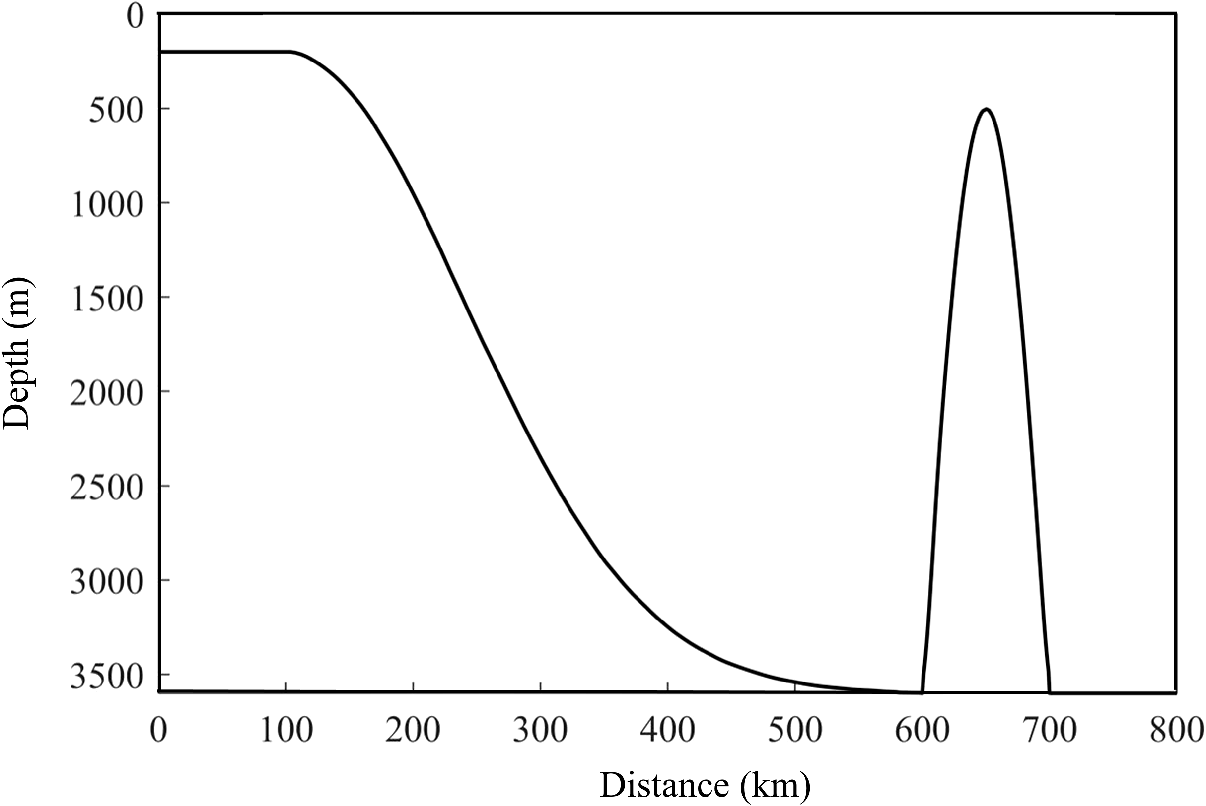
Simplified topography employed for ISW simulation.
The initial model temperature, salinity and buoyancy frequency profiles are derived from World Ocean Atlas 2018 (Garcia et al., 2019) in horizontally uniform conditions, as shown in Figure 2. To ensure numerical stability while maintaining computational efficiency, the time step was set to 3 s to satisfy the Courant–Friedrichs–Lewy (CFL) condition.
Figure 2
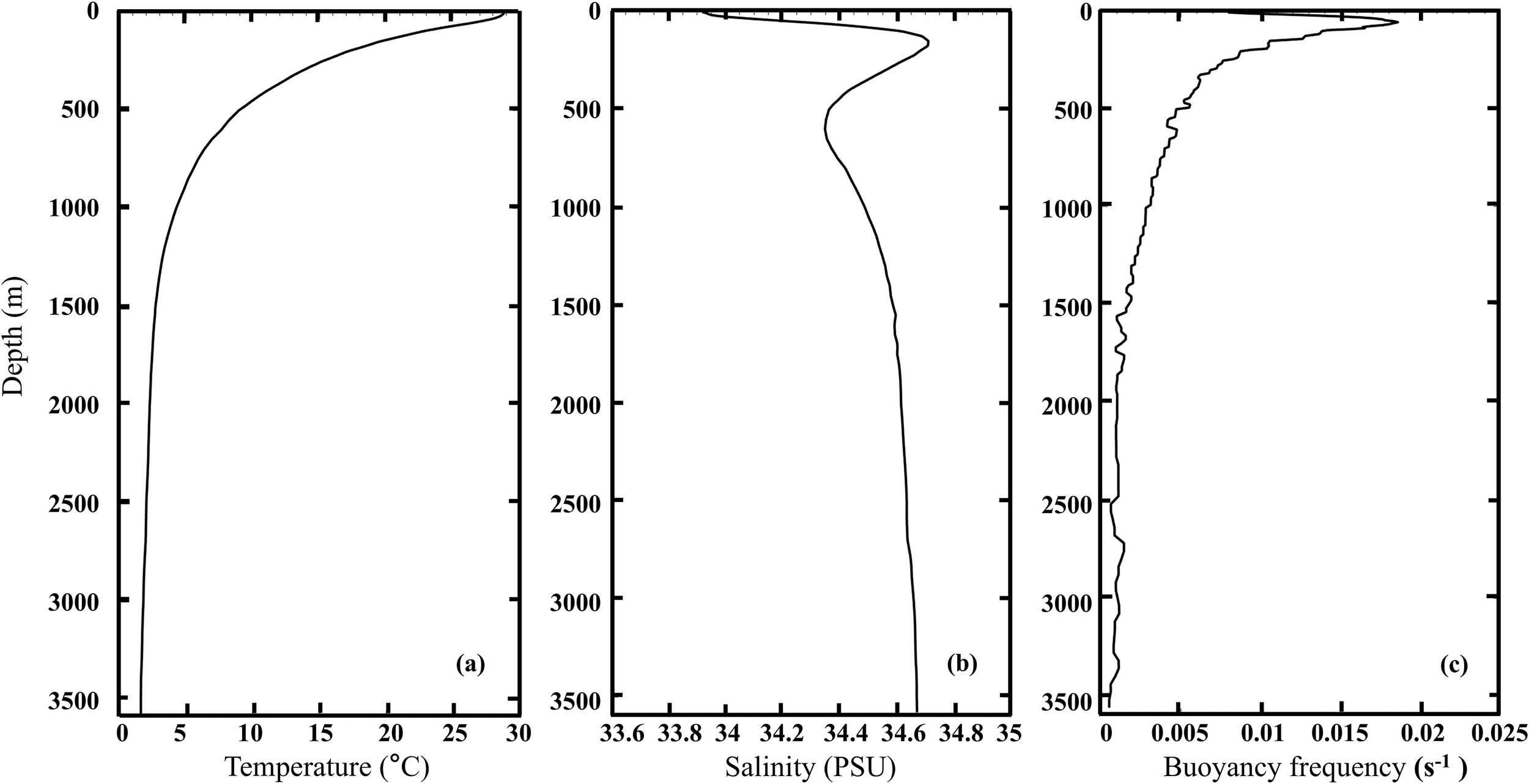
Profiles of initial conditions: (a) temperature; (b) salinity; (c) buoyancy frequency.
The model is driven by adding periodical barotropic tides at the east-west open boundary of the simulation area (Cai et al., 2021), with flow velocity utide versus time as Equation 25:
where U0 is the amplitude of the barotropic tides; Ttide is the tidal period. The M2 constituent is selected to drive the model, with a period of 12.42 h and amplitude of the periodically varying horizontal barotropic tides is 0.2 m/s. The horizontal diffusion coefficient of the model is taken as κh = 10-5 m2/s, the horizontal and vertical viscosity coefficients are taken as Ah = 10-5 m2/s and Az = 10-4 m2/s. The K-Profile Parameterization (KPP) scheme is adopted as the vertical mixing parameterization scheme in this paper (Wang et al., 2014). This paper uses the presented model to simulates the ISW propagation process, and outputs the ISW-induced dynamic water pressure and bed shear stress as inputs for the seabed response.
3.2 ISW model verification
The temperature field after the sixth M2 tidal cycle is outputted in Figure 3. A large-amplitude ISW is generated by the interaction of tidal currents and topography within the model, with an amplitude of 94 m during its propagation towards the continental slope. This simulated amplitude is very close to the amplitude 91 m interpreted from the observed ISW-associated temperature field at 20.83°N (Huang and Zhao, 2014). In addition, the simulated propagation speed of the ISW towards 119°E is about 2.77 m/s, which is also very consistent with the average propagation speed of 2.92 m/s interpreted from the MODIS image (Huang and Zhao, 2014). Therefore, comparisons of both amplitude and propagation speed demonstrate that the simulation of ISWs in this paper has a high degree of consistency with the observations. This agreement verifies the accuracy and reliability of the proposed model in effectively simulating the characteristics and propagation process of ISWs in the northern SCS.
Figure 3
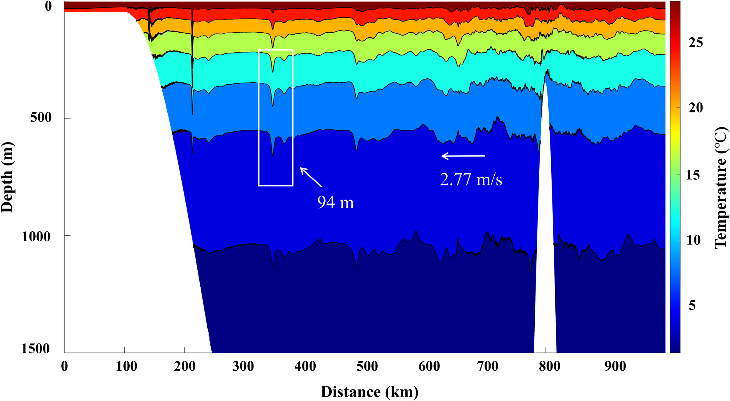
The simulated temperature field after the sixth M2 tidal cycle.
Based on the proposed model, the ISW-induced vertical pressure acting on the seabed surface at water depth 180 m is illustrated in Figure 4. As a large-amplitude ISW packet passing through the seabed, a bottom pressure fluctuation exceeding 5 kPa occurs, with the shape of the fluctuation resembling the propagation characteristics of ISWs. In the northern SCS, Ma et al. (2016) captured a depressed ISWs-induced large-amplitude pressure perturbation of about 3 kPa near the seabed at water depth 175 m. The measurements were acquired using five pressure sensors at about 10 m above the seabed, and the pressure signal was distinguished from other hydrodynamic through high-pass filterings. Tian et al. (2024a) observed the seabed methane release processes at water depth 600 m under ISWs, indicating that the arrival of ISWs coincided with the seabed pressure increasing by 1~2 kPa. The pressure are obtained using paroscientific pressure transducer with a sampling rate of 10 s, and the ISW-induced signal are identified by the symmetric flow velocity structure in the vertical flow velocity profile. The parameters of the above-mentioned field observations and the simulated ISW-induced pressure are showed in Table 1. The order of magnitudes of the pressure outputted by the presented model are consistent with the observations. The simulated values are nearly the same as the observed ones at similar water depth, further validating the model’s reliability in describing the ISW-induced bottom pressure fields.
Figure 4
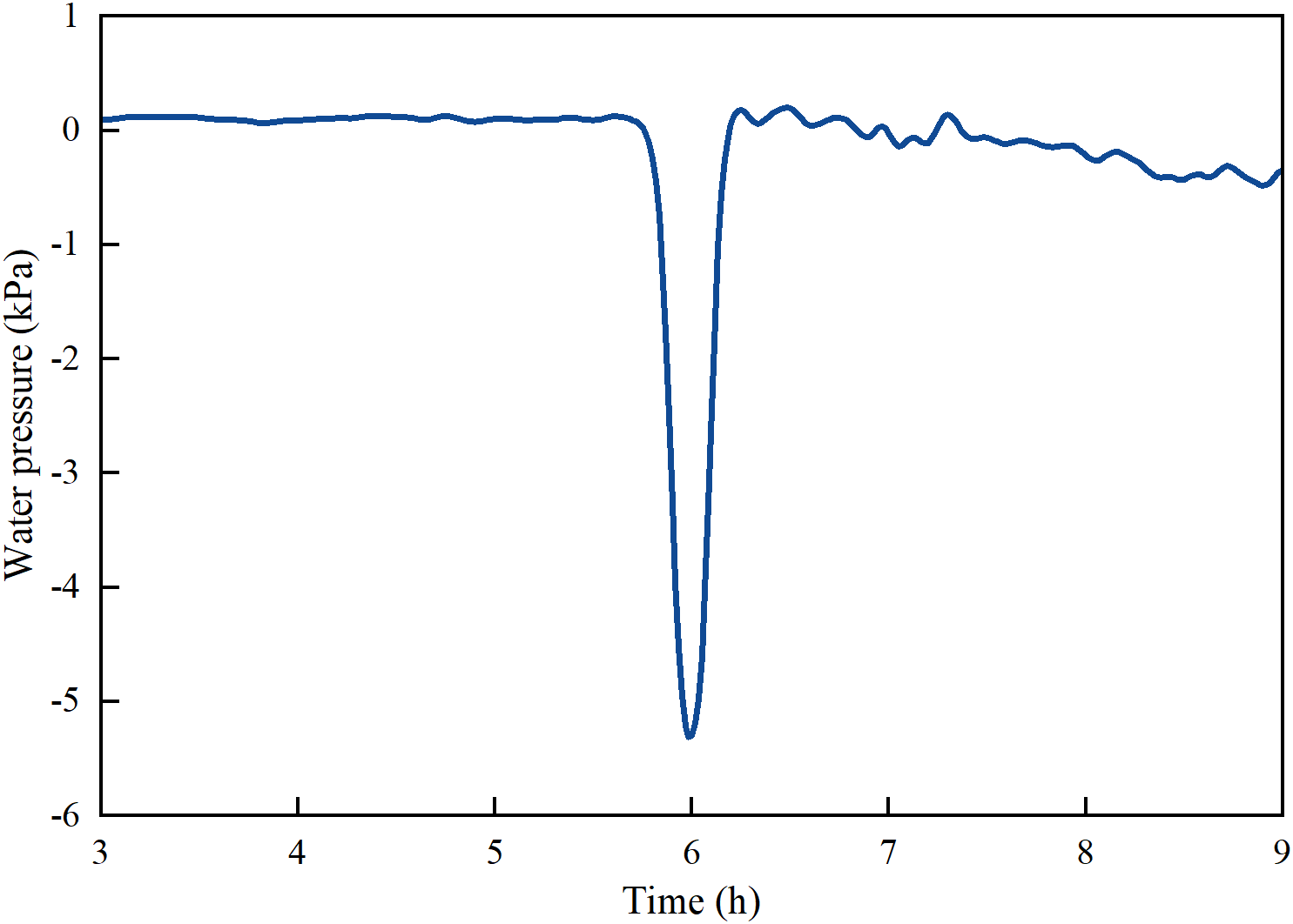
Simulated ISW-induced vertical pressure at water depth 180 m.
Table 1
| Experiments | Water depth (m) | Period (min) | Amplitude (m) | Pressure (kPa) |
|---|---|---|---|---|
| Ma et al. (2016) | 175 | 20 | 80 | 3 |
| Tian et al. (2014a) | 600 | 10~20 | 100 | 1~2 |
| Simulation by the presented model | 180 | 20 | 94 | 5 |
Comparison of observed and simulated ISW-induced pressure.
3.3 Seabed model setup
As this paper specifically examines the ISW-induced seabed response and sand wave migration within a water depth range of 80~250 m. The seabed model is initially configured with a water depth of 180 m and a time step of 1 s. According to the typical types of seabed soil in the northern SCS (Zhang, 2021), a unified sediment grain size parameter of D50 = 0.065 mm for silt sand is preliminary used in the present experiments. The seabed thickness is taken as 40 m because the ISW-induced pressure is negligibly at 40 under seabed surface. The vertical spatial step is taken as 0.5 m. The parameters are taken as α=0.246 and β=-0.165 (Jeng et al., 2007). Other parameters for the seabed model are listed in Table 2 according to the literatures with similar conditions of the present study (Chowdhury et al., 2006; Qi and Gao, 2015).
Table 2
| Parameters | Value |
|---|---|
| Median grain size D50 | 0.065 mm |
| Particle density | 2.68 g/cm3 |
| Water density | 1 g/cm3 |
| Porosity n | 0.45 |
| Poisson’s ratio | 0.49 |
| Saturation Sr | 0.98 |
| Penetration rate Ks | 1×10⁻⁴ m/s |
| Modulus of elasticity E | 30 MPa |
Basic soil parameters in this paper.
4 Results and discussion
4.1 ISW-induced transient and accumulated pore pressure
This paper simulates a single ISW with amplitude of 94 m and outputs the ISW-induced pressure variations at a water depth of 180 m. ISW may induce either transient pore pressure or accumulated pore pressure response of the seabed. On the one hand, depressed ISWs generate the most significant negative pressure below the wave troughs, inducing transient pore pressure and upward seepage gradients within the seabed. However, the depth and duration of their impact are limited. One the other hand, the ISW packet typically comprises a sequence of successive ISWs. Similar to surface waves, the successive sub-waves can induce pore pressure buildup in under-consolidated seabed. The following section quantifies the pore pressure response induced by individual wave packets and continuous sub-waves during the passage of ISWs, and further discusses the contribution of the two pore pressure responses.
The ISW-induced vertical pressure at seabed surface can penetrate into a specific depth within the seabed, resulting in the development of EPP. The transient pore pressure at depths of 5 cm below the seabed surface is depicted in Figure 5. During the 30-min interval in which a single large-amplitude ISW traverses the area, a seabed pore pressure response of with maximum negative value 1.64 kPa is generated (negative value at wave trough phase). The transient pore pressure variations exhibit a strong correlation with the waveform of the ISW, thereby providing additional evidence for the vertical impact of the ISW on the seabed.
Figure 5
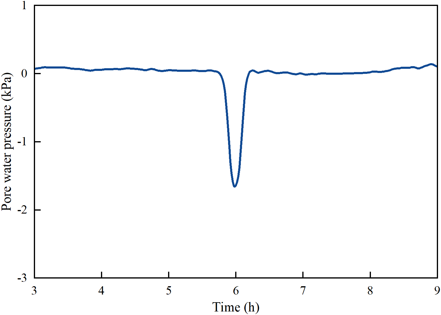
Temporal variation of transient pore pressure induced by ISWs (5 cm below the bed surface).
The change of ISWs-induced accumulated pore pressure with depth of seabed is shown in Figure 6. Assuming the ISW packets propagate with a constant amplitude and constant interval Tisw, Nisw=t/Tisw represents the number of ISW in the packet (Su et al., 2017). The accumulated pore pressure increases as the number of ISW increase, with the maximum value reaching approximately 4 kPa at depth of 12 m. Comparing with the transient response that mainly occurs within the upper layer of seabed, the maximum accumulated pore pressure occurs deeper.
Figure 6
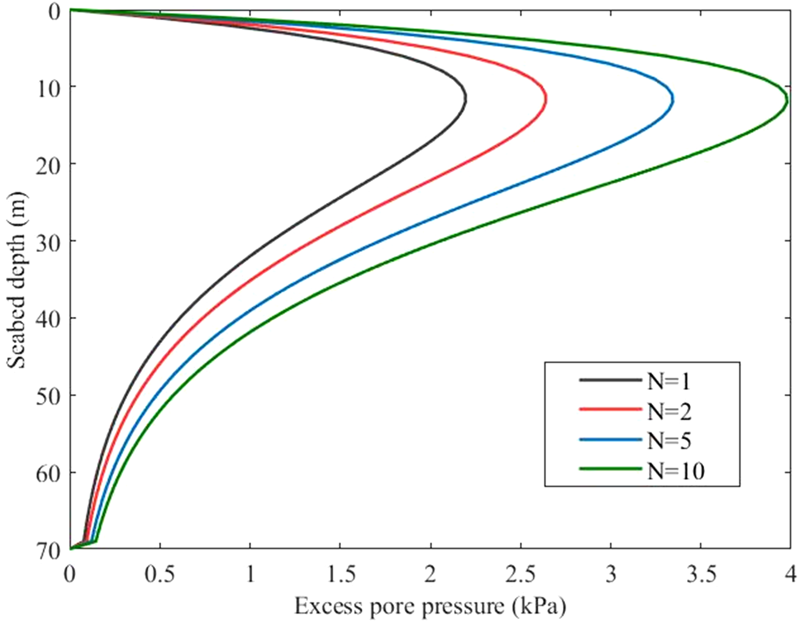
Variation of accumulated pore pressure on the seabed under the action of ISWs at different propagation times.
The EPP response is represented by the EPP ratios, which is commonly known as the ratio r between EPP and the initial effective stress, that is (Do et al., 2023). According to one-dimensional liquefaction criterion, the seabed soil will be completely liquefied when the EPP offsets the effective stress of the overlying soil (Liu, 2008). The transient EPP is defined as p ′=-(p0-p), where p0 is the ISW-induced pressure at the seabed surface. The variation of EPP ratio with seabed depth is of both transient and accumulated response are shown in Figure 7 and Figure 8. Transient liquefaction occurs predominantly in the uppermost layer of the seabed, with a liquefaction depth of approximately 0.19 m. Athough the accumulated EPP ratio reaches its maximum value of 0.08 in the surface layer of the seabed, is far from reaching the threshold for liquefaction.
Figure 7
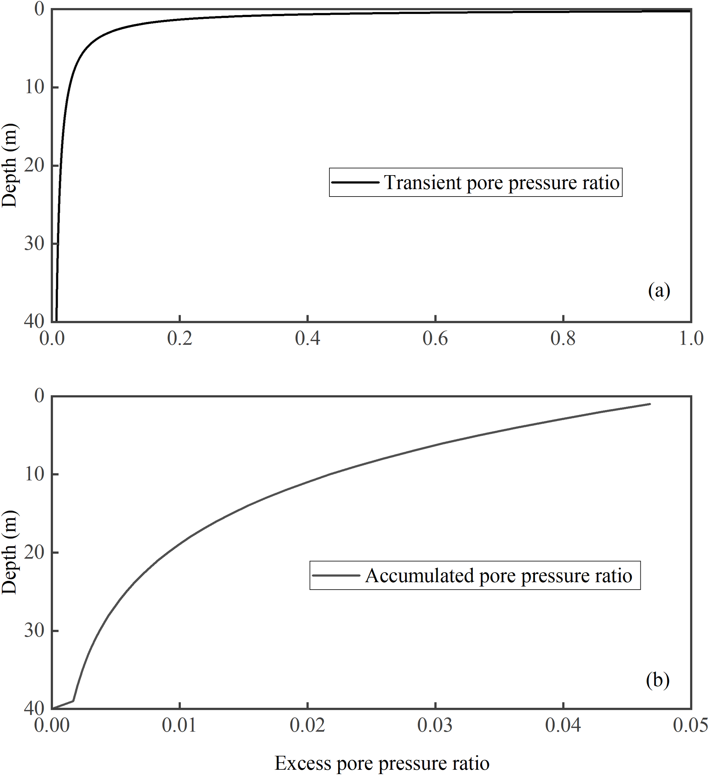
ISW induced excess pore pressure ratio with depth: (a) transient; (b) accumulated.
Figure 8
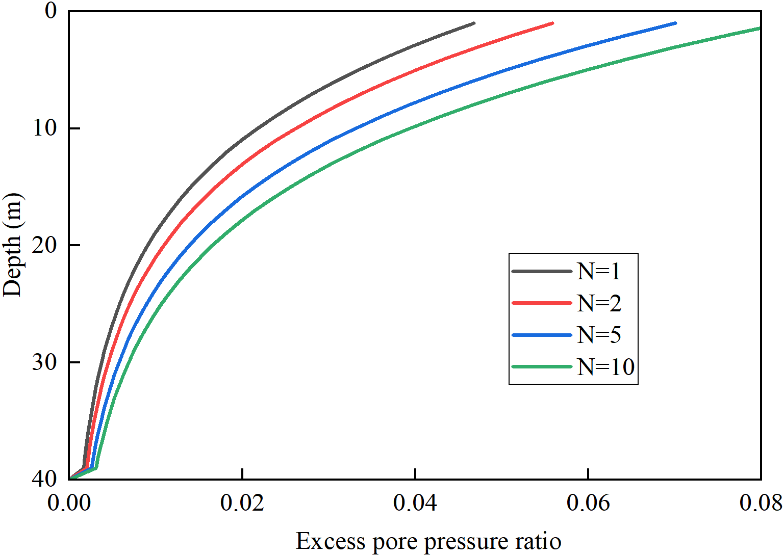
Accumulated excess pore pressure ratio with depth under different ISW cycles.
The explanation of the different response features of the transient and accumulated pore pressure can be categorized into three aspects. Firstly, ISWs are generated by a significant vertical fluctuations between the density layers of seawater. However, the densities of the seawater of the upper and lower layers are very close. The vertical pressure changes induced by the ISW on the seabed surface are relatively minor. This results in a limited impact on the response of pore pressure within the seabed; Secondly, the wave period of ISW is typically longer, while the duration of their action is often shorter. Consequently, a significant proportion of pore pressure accumulated by former ISW would dissipate before the subsequent ISW, making it difficult for pore pressure to accumulate under ISW series. Additionally, the sand wave is predominantly composed of fine sand silt sand, and a small proportion of clay (Geng et al., 2017). The higher permeability makes the pore water easier to get in and out of the seabed, facilitating the rapid penetration of water through the soil’s pore structure and contributing to the fast dissipation of the pore pressure.
4.2 Seepage force due to transient and accumulated response
Pore pressure gradients and seepage forces are critical factors in the analysis of seabed response (Liu et al., 2017). ISWs generate pressure on the seabed surface within a short duration, resulting in an accumulation of pore pressure within the seabed and generating an upward seepage force. In the case of a single ISW passing through, the transient pore pressure gradient leads to temporal variations in the seepage force acting on the seabed surface in Figure 9a. The seepage force increases significantly as the propagation of ISWs on the whole. To be specific, the seepage force exhibits different patterns at different depth. The greatest increase of seepage force 4.6 Pa appears at 1.0 cm, and the peak seepage force decrease rapidly with depth to 2.0 Pa at 10.0 cm. The changes in seepage forces are closely related to pore pressure variations, and their magnitude may be influenced by the ISW-induced dynamic pressure fields. Additionally, the variation of seepage force at depth 180 m in response to accumulated pore pressure is also depicted in Figure 9b. During an ISW cycle, the seepage force gradually increases from 0 Pa to 0.068 Pa at 10.0 cm, and its overall trend is consistent with the accumulated pore pressure. However, the maximum value of accumulated response-induced seepage force is much smaller, maybe two orders of magnitude smaller than the transient response-induced seepage force in the surface seabed layer.
Figure 9
ISW induced seepage force with time: (a) transient; (b) accumulated (during a single ISW cycle).
The above results indicate that the transient pore pressure response dominates the ISW-induced internal response of seabed, whereas the accumulated pore pressure response exerts a relatively minimal impact. Therefore, only the transient pore pressure and seepage force caused by a single extremely large-amplitude ISW is considered, while the accumulated response of seabed due to sequent ISWs is ignored when analyzing the ISWs-induced sand wave migration.
4.3 Influence of seepage forces on sediment erosion
As a critical parameter for assessing sediment initiation, the variation in the critical incipient shear stress (CISS) of sediment serves as an indicator of the impact of seepage forces on the bed surface response. Figure 10 illustrates the calculated CISS of sediment within 50 cm beneath the bed surface during one ISW cycle, in which the impacts of seepage force are taken into account. The CISS exhibits a minimum value of 0.38 Pa at depth of 5 cm, then increases gradually with the seabed depth to reach 0.94 Pa at 50 cm below the bed surface, ultimately approaching the stable value 1.2 Pa without considering the seepage force. It should be noted that the bigger CISS, the harder for the sediment to be initiated. Thus the ISW-induced seepage force significantly reduces the CISS of sediment, and in turn promotes the initiation of sediment in the upmost seabed layer. This finding can also be corroborated by the results from the flume experiments conducted by Tian et al. (2022, 2023).
Figure 10
Critical incipient shear stress with and without considering the ISW-induced transient seepage force.
Figure 11 shows the ISW-induced maximum bottom shear stress and the minimum CISS that considering the seepage force at different seabed depths. Under normal conditions, that is, when the ISW-induced transient liquefaction and seepage force is not considered, the maximum ISW-associated bed shear stress of 0.94 Pa is smaller than the CISS 1.18 Pa, indicating that the sediment cannot be initiated. However, when introducing the transient EPP and corresponding seepage force, the CISS of the sediment is reduced to 0.38 Pa. This value falls below the ISW-associated maximum bed shear stress, thereby the sediment can be initiated. The bed shear stress is approximately equal to the CISS at 0.49 m, leading to an equilibrium state in sediment initiation. In other words, the ISW-induced critical erosion depth of sand seabed is 0.49 m.
Figure 11
Variations in critical incipient shear stress amplitude and bed shear stress at different seabed depths after considering seepage force.
4.4 Impact of ISW-induced internal-surface coupling response on bed load transport rates
The ISW-induced seabed internal-surface coupling response process, i.e., the ISW can generate EPP and upward seepage force acting on the sediment particles, and thus promote the incipient motion of sediment at seabed surface. Among them, the bed shear stress is calculated based on ISW-induced near-bottom velocities during its passage, as tidal currents not taken into consideration. The critical incipient shear stress are considered dynamically during ISWs passage, showing strong correlation with seepage force(See Section 4.3). Based on this, the bed load transport rates in a single cycle of the ISW is calculated according to Equations 23, 24, in which only the time duration for the bed shear stress exceeding the critical incipient condition makes sense. By considering the ISW-induced internal-surface coupling response, the bed load transport rates increases to 8.22×10⁻⁴ kg·m-1·s-1 in a single cycle of the ISW.
This paper investigates different waterdepth ranging from 150 to 1000 m on the upper slope and outer continental shelf area of northern SCS. Figure 12 shows that changes in water depth affect the bed load transport rates under ISWs. The maximum bed load transport rates occurs at a water depth of 400 m. In shallower conditions (<400 m), seabed mobility diminishes progressively with decreasing depth. It correlates with ISW energy reduction caused by shoaling and fission processes during upslope propagation (Tan et al., 2019; Hartharn-Evans et al., 2022). In deeper conditions (>400 m), seabed mobilization gradually strengthens with decreasing depth. This is because ISWs are closer to the seabed, resulting in enhanced impacts on bed load transport rates. At water depths exceeding 700 m, the bedload transport rates are significantly reduced, leading to attenuated migration activity under ISWs. It implies the critical depth constraints on ISW-seabed interactions. Future research should integrate high-resolution numerical models and long-term field observations to better validate sand wave migration dynamics at different water depths.
Figure 12
Bed load transport rates versus water depth under ISWs.
The results suggest that ISWs play an important role in the migration of sand wave on the upper slope and outer continental shelf in the northern SCS. ISWs-induced pore pressure gradient can remarkably enhance the seepage force, reducing the CISS of sediment particles, and thus promoting the sediment erosion and bed load transport. During the passage of ISW event, the rapid increase in near-bottom flow velocity can result in displacement of sand waves within a short period. The frequent ISW events in the northern SCS can thereby induce remarkable macroscopic sand wave migration. The results of this paper show the certain contribution of ISWs on sand wave migration on the upper slope and outer continental shelf. However, more in-situ observations on the ISW-related hydrodynamic and sediment dynamic of sand waves are still needed to further verify the present model. In addition, due to the complex geometrical characteristics and migration patterns of different sand wave fields, the impact of ISW events may superimpose with the influences of astronomic tide, internal tide, and typhoon events. The superimposed effects can form a complex bottom flow and shear stress field, making the sand wave migration present characteristics such as complex migrating directions. The presented model analyzes the bed load transport induced by ISWs, and further research are needed to consider the superimposed influence of different driving forces.
5 Conclusion
This paper proposes a model to evaluate the ISW-induced bed load transport on the upper slope and out continental shelf in northern SCS, in which the internal-surface coupling response of seabed under ISW is particularly considered. The main conclusions are as follows.
1. A coupling response exists between the internal and surface of seabed under the action of ISWs. ISWs can induce EPP in the seabed, resulting in upward seepage force acting on the sediment particles, and thus reduce the critical incipient shear stress. This process promotes sediment initiation and transport at the seabed surface. The maximum value of accumulated response-induced seepage force is two orders smaller than the transient one in the surface seabed layer. The ISW-induced transient EPP dominates the internal response of seabed due to ISWs. Transient liquefaction occurs at the uppermost seabed layer due to ISW, while the ISW-induced erosion depth can be twice if the seepage force is added to the sediment force equilibrium equation.
2. The ISW-induced vertical pressure fluctuation and horizontal shear stress near the seabed can be effectively obtained based on the numerical model of MITgcm. By incorporating these external driving forces with the internal-surface coupling response of seabed, the bed load transport rate is thus reasonably calculated. The results suggest that ISWs play an important role in the migration of sand wave on the upper slope and outer continental shelf in the northern SCS. Although more in-situ observations are still needed to further calibrate and verify the present model. Other hydrodynamics such as astronomic tide, internal tide and typhoon events may also contribute to the migration of different sand wave fields on the upper slope and outer continental shelf in northern SCS. The present model can be adapted to incorporate additional forcings as future data become available.
Statements
Data availability statement
The raw data supporting the conclusions of this article will be made available by the authors, without undue reservation.
Author contributions
YL: Writing – original draft, Data curation, Validation, Visualization, Investigation, Conceptualization, Methodology, Software, Writing – review & editing, Formal Analysis. HW: Writing – original draft, Funding acquisition, Resources, Software, Project administration, Supervision, Methodology, Writing – review & editing. HC: Supervision, Funding acquisition, Resources, Writing – review & editing. YJ: Resources, Funding acquisition, Writing – review & editing, Supervision, Data curation, Project administration.
Funding
The author(s) declare that financial support was received for the research and/or publication of this article. This work was supported by the National Key Research and Development Program of China (2023YFC3107901), and the National Natural Science Foundation of China (41702307).
Conflict of interest
The authors declare that the research was conducted in the absence of any commercial or financial relationships that could be construed as a potential conflict of interest.
Generative AI statement
The author(s) declare that no Generative AI was used in the creation of this manuscript.
Publisher’s note
All claims expressed in this article are solely those of the authors and do not necessarily represent those of their affiliated organizations, or those of the publisher, the editors and the reviewers. Any product that may be evaluated in this article, or claim that may be made by its manufacturer, is not guaranteed or endorsed by the publisher.
References
1
Alford M. H. Peacock T. MacKinnon J. A. Nash J. D. Buijsman M. C. Centurioni L. R. et al . (2015). The formation and fate of internal waves in the South China Sea. Nature521, 65–69. doi: 10.1038/nature14399
2
Bai Y. Yang X. Tian Q. Zhang B. (2009). Evolution characteristics of seabed sand wave in northern South China Sea. J. Hydraulic Eng.40941–947+955. doi: 10.13243/j.cnki.slxb.2009.08.012
3
Blondeaux P. Vittori G. (2016). A model to predict the migration of sand waves in shallow tidal seas. Continent. Shelf Res.112, 31–45. doi: 10.1016/j.csr.2015.11.011
4
Cacchione D. A. Drake D. E. (1986). Nepheloid layers and internal waves over continental shelves and slopes. Geo-Marine Lett.6, 147–152. doi: 10.1007/BF02238085
5
Cai S. (2015). Numerical model of internal solitary waves and its application to the South China Sea (Beijing: Ocean Press).
6
Cai S. Wu Y. Xu J. Chen Z. Xie J. He Y. (2021). On the generation and propagation of internal solitary waves in the southern Andaman Sea: A numerical study. Scie. Sinica(Terrae)51, 2001–2014. doi: 10.1007/s11430-020-9802-8
7
Chen B. (2022). Two-dimensional numerical study of internal solitary waves in thenorthern South China Sea (Dalian, China: Dalian University of Technology). doi: 10.26991/d.cnki.gdllu.2022.000243
8
Chen C. Y. Hsu J. R. C. (2005). Interaction between internal waves and a permeable seabed. Ocean Eng.32, 587–621. doi: 10.1016/j.oceaneng.2004.08.010
9
Chowdhury B. Dasari G. R. Nogami T. (2006). Laboratory study of liquefaction due to wave–seabed interaction. J. Geotech. Geoenviron. Eng.132, 842–851. doi: 10.1061/(ASCE)1090-0241(2006)132:7(842
10
Do T. M. Laue J. Mattsson H. Jia Q. (2023). Excess pore water pressure generation in fine granular materials under undrained cyclic triaxial loading. Geo-Engineering14, 8. doi: 10.1186/s40703-023-00185-y
11
Dou G. Dong F. Dou X. Li Z. (1995). Mathematical modeling of estuarine coastal sediment. Sci. In China(Series A)25 (9), 995–1001. doi: 10.1360/za1995-25-9-995
12
Droghei R. Falcini F. Casalbore D. Martorelli E. Mosetti R. Sannino G. et al . (2016). The role of Internal Solitary Waves on deep-water sedimentary processes: the case of up-slope migrating sediment waves off the Messina Strait. Sci. Rep.6, 36376. doi: 10.1038/srep36376
13
Feng W. Xia Z. (1993). Study on the stability of seafloor sand waves in the northern part of the South China Sea. Gresearch Eol. South China Sea5, 26–42. +T003.
14
Gao S. (2009). Morphology and migration characteristics of large benthic, coastal and desert dunes. Earth Sci. Front.16, 13–22. doi: 10.3321/j.issn:1005-2321.2009.06.002
15
Garcia H. E. Boyer T. P. Baranova O. K. Locarnini R. A. Mishonov A. V. Grodsky A. et al (2019). World Ocean Atlas 2018: Product Documentation. Ed. MishonovA.National Centers for Environmental Information. (1315 East-West Highway Silver Spring, MD: National Centers for Environmental Information).
16
Geng M. Song H. Guan Y. Bai Y. Liu S. Chen Y. (2017). The distribution and characteristics of very large subaqueous sand dunes in the Dongsha region of the northern South China Sea. Chin. J. Geophy.60, 628–638. doi: 10.6038/cjg20170217
17
Hartharn-Evans S. G. Carr M. Stastna M. Davies P. A. (2022). Stratification effects on shoaling internal solitary waves. J. Fluid Mech.933, A19. doi: 10.1017/jfm.2021.1049
18
Huang X. Zhao W. (2014). Information of internal solitary wave extracted from MODIS image:a case in the deep water of northern south China sea. Period. Ocean Univ. China44, 19–23. doi: 10.16441/j.cnki.hdxb.2014.07.003
19
Jeng D. S. Seymour B. R. Li J. (2007). A new approximation for pore pressure accumulation in marine sediment due to water waves. Num. Anal. Meth. Geomech.31, 53–69. doi: 10.1002/nag.547
20
Leckie S. H. F. Mohr H. Draper S. McLean D. L. White D. J. Cheng L. (2016). Sedimentation-induced burial of subsea pipelines: Observations from field data and laboratory experiments. Coast. Eng.114, 137–158. doi: 10.1016/j.coastaleng.2016.04.017
21
Liang J. Li X. M. Sha J. Jia T. Ren Y. (2019). The lifecycle of nonlinear internal waves in the northwestern south China sea. J. Phys. Oceanogr.49, 2133–2145. doi: 10.1175/JPO-D-18-0231.1
22
Lin M. Fan F. Li Y. Yan J. Jiang W. Gong D. (2009). Observation and theoretical analysis for the sand-waves migration in the North Gulf of South China Sea. Chin. J. Geophy.52, 776–784.
23
Liu X. Jia Y. Zheng J. Wen M. Shan H. (2017). An experimental investigation of wave-induced sediment responses in a natural silty seabed: New insights into seabed stratification. Sedimentology64, 508–529. doi: 10.1111/sed.12312
24
Liu Z. (2008). Study on Wave-induced Response of Progressive Pore Pressure and Liquefaction in Seabed (Dalian, China: Dalian University of Technology).
25
Lu Y. Lu Y. Li S. (2011). Bed load transport with bed seepage. Adv. Water Sci.22, 215–221. doi: 10.14042/j.cnki.32.1309.2011.02.012
26
Luan X. Peng X. Wang X. Qiu Y. (2010). Characteristics of sand waves on the northern south China sea shelf and its formation. Acta Geol. Sin.84, 233–245. doi: 10.19762/j.cnki.dizhixuebao.2010.02.009
27
Ma X. Yan J. Hou Y. Lin F. Zheng X. (2016). Footprints of obliquely incident internal solitary waves and internal tides near the shelf break in the northern South China Sea. J. Geophysical Res.: Oceans121, 8706–8719. doi: 10.1002/2016jc012009
28
McDougal W. G. Tsai Y. T. Liu P. L.-F. Clukey E. C. (1989). Wave-induced pore water pressure accumulation in marine soils. J. Offshore Mechan. Arctic Eng.111, 1–11. doi: 10.1115/1.3257133
29
Miramontes E. Jouet G. Thereau E. Bruno M. Penven P. Guerin C. et al . (2020). The impact of internal waves on upper continental slopes: insights from the Mozambican margin (southwest Indian Ocean). Earth Surf Processes Landf45, 1469–1482. doi: 10.1002/esp.4818
30
Nemeth A. Hulscher S. de Vriend H. (2003). Offshore sand wave dynamics, engineering problems and future solutions. Pipeline Gas J. 230 (4), 67–69. doi: 10.1061/(ASCE)0733-9372(2004)130:1(37)
31
Qi W. G. Gao F. P. (2015). A modified criterion for wave-induced momentary liquefaction of sandy seabed. Theor. Appl. Mechan. Lett.5, 20–23. doi: 10.1016/j.taml.2015.01.004
32
Qian N. Wan Z. (1983). Sediment Dynamics. 1st Edn (Beijing: Science Press). Available online at: https://book.sciencereading.cn/shop/book/Booksimple/show.do?id=B2252DFB8C35949A398359E5EDCA22F4B000.
33
Qiu Z. Fang W. (1999). Vertical variation of spring sea currentin northern South China Sea. Tropic Oceanol.18 (4), 33–40.
34
Reeder D. B. Ma B. B. Yang Y. J. (2011). Very large subaqueous sand dunes on the upper continental slope in the South China Sea generated by episodic, shoaling deep-water internal solitary waves. Mar. Geol.279, 12–18. doi: 10.1016/j.margeo.2010.10.009
35
Ren B. Wang Z. Liang B. Xie B. Lu Y. Qi J. et al . (2025). Dynamic response mechanism of sand waves to polarity conversion in internal solitary waves on the northern slope of the South China Sea. Ocean Eng.32, 1–16. Available at: https://link.cnki.net/urlid/32.1423.P.20250320.1507.002
36
Rivera Rosario G. A. Diamessis P. J. Jenkins J. T. (2017). Bed failure induced by internal solitary waves. JGR Oceans122, 5468–5485. doi: 10.1002/2017JC012935
37
Rubin D. M. Hunter R. E. (1982). Bedform climbing in theory and nature. Sedimentology29, 121–138. doi: 10.1111/j.1365-3091.1982.tb01714.x
38
Seed H. B. Rahman M. S. (1978). Wave-induced pore pressure in relation to ocean floor stability of cohesionless soils. Mar. Geotechnol.3, 123–150. doi: 10.1080/10641197809379798
39
Su Y. Qiao L. Guo X. Tian Z. (2017). Analysis of internal solitary wave-induced seabed stability of sediments in the northern South China Sea. Geotechn. Invest. Survey.45, 30–36.
40
Sun Y. (2021). Study on Formation and CharacteristicScale of Submarine Sand Waves UnderTidal Current and Combined Wave-currentConditions (Tianjin, China: Tian University). doi: 10.27356/d.cnki.gtjdu.2021.002665
41
Tan D. Zhou J. Wang X. Wang Z. (2019). Combined effects of topography and bottom friction on shoaling internal solitary waves in the South China Sea. Appl. Math. Mech.-Engl. Ed.40, 421–434. doi: 10.1007/s10483-019-2465-8
42
Thomas J. A. Lerczak J. A. Moum J. N. (2016). Horizontal variability of high-frequency nonlinear internal waves in Massachusetts Bay detected by an array of seafloor pressure sensors. JGR Oceans121, 5587–5607. doi: 10.1002/2016JC011866
43
Tian Z. Chen T. Yu L. Guo X. Jia Y. (2019). Penetration depth of the dynamic response of seabed induced by internal solitary waves. Appl. Ocean Res.90, 101867. doi: 10.1016/j.apor.2019.101867
44
Tian Z. Huang J. Song L. Zhang M. Jia Y. Yue J. (2024a). The Interaction between internal solitary waves and submarine canyons. J. Mar. Environ. Eng.11, 129–139. doi: 10.32908/JMEE.v11.2024050101
45
Tian Z. Huang J. Xiang J. Zhang S. (2024b). Suspension and transportation of sediments in submarine canyon induced by internal solitary waves. Phys. Fluids36, 022112. doi: 10.1063/5.0191791
46
Tian Z. Jia Y. Chen J. Liu J. P. Zhang S. Ji C. et al . (2021). Internal solitary waves induced deep-water nepheloid layers and seafloor geomorphic changes on the continental slope of the northern South China Sea. Phys. Fluids33, 053312. doi: 10.1063/5.0045124
47
Tian Z. Jia L. Xiang J. Yuan G. Yang K. Wei J. et al . (2023). Excess pore water pressure and seepage in slopes induced by breaking internal solitary waves. Ocean Eng.267, 113281. doi: 10.1016/j.oceaneng.2022.113281
48
Tian Z. Liu C. Ren Z. Guo X. Zhang M. Wang X. et al . (2022). Impact of seepage flow on sediment resuspension by internal solitary waves: parameterization and mechanism. J. Oceanol. Limnol.41, 444–457. doi: 10.1007/s00343-022-2001-9
49
Tong L. Zhang J. Chen N. Lin X. He R. Sun L. (2024). Internal solitary wave-induced soil responses and its effects on seabed instability in the South China Sea. Ocean Eng.310, 118697. doi: 10.1016/j.oceaneng.2024.118697
50
Wang S. Li D. (1994). Dynamic analysis of seafloor sand waves on the shelf slope and continental slope in the Pearl River Estuary Basin, South China Sea. Acta Oceanol. Sin.16 (6), 122–132. doi: 10.3321/j.issn:0253-4193.1994.06.003
51
Wang H. Liu H. (2015). A simplified analysis method for residual pore pressure response of silty seabed under wave loads. Period. Ocean Univ. China45, 75–80. doi: 10.16441/j.cnki.hdxb.20140253
52
Wang L. Wang Z. Lin T. Zuo J. (2014). Review of vertical mixing parameterization in ocean climate modeling. Mar. Forecasts31, 93–104. doi: 10.11737/j.issn.1003-0239.2014.05.015
53
Williams S. J. Jeng D.-S. (2007). The effects of a porous-elastic seabed on interfacial wave propagation. Ocean Eng.34, 1818–1831. doi: 10.1016/j.oceaneng.2007.02.002
54
Wu J. Hu R. Zhu L. Ma F. Liu J. (2006). Study on the seafloor sandwaves in the northern south China sea. Period. Ocean Univ. China36 (6), 1019–1023. doi: 10.16441/j.cnki.hdxb.2006.06.033
55
Xia H. Liu Y. Yang Y. (2009). Internal-wave characteristics of strong bottom currents at the sand-wave zone of the northern South China Sea and its role in sand-wave motion. J. Trop. Oceanogr.28, 15–22. doi: 10.11978/j.issn.1009-5470.2009.06.015
56
Xie L. Chen L. Zheng Q. Wang G. Yu J. Xiong X. et al . (2024). Mechanisms of reappeared period shifts of internal solitary waves based on mooring array observations in the northern south China sea. JGR Oceans129, e2023JC020389. doi: 10.1029/2023JC020389
57
Yang Y. Huang X. Zhou C. Zhang Z. Zhao W. Tian J. (2022). Three-dimensional structures of internal solitary waves in the northern south China sea revealed by mooring array observations. Prog. Oceanogr.209, 102907. doi: 10.1016/j.pocean.2022.102907
58
Zen K. Jeng D. Hsu J. R. C. Ohyama T. (1998). Wave-induced seabed instability: difference between liquefaction and shear failure. Soils Foundations38, 37–47. doi: 10.3208/sandf.38.2_37
59
Zeng K. Lyu R. Li H. Suo R. Du T. He M. (2024). Studying the internal wave generation mechanism in the northern south China sea using numerical simulation, synthetic aperture radar, and in situ measurements. Remote Sens.16, 1440. doi: 10.3390/rs16081440
60
Zhang Y. (2021). Numerical Simulation of Submarine Sand Waves on the Continental Slope of the Northern South China Sea under the Internal Wave Current (Tianjin, China: Tian University). doi: 10.27356/d.cnki.gtjdu.2021.000806
61
Zhang H. Ma X. Zhuang L. Yan J. (2019). Sand waves near the shelf break of the northern South China Sea: morphology and recent mobility. Geo-Mar Lett.39, 19–36. doi: 10.1007/s00367-018-0557-3
62
Zhang H. Zhuang L. Yan J. Ma X. (2017). Progress of sand waves and internal waves research in sea areawest of the Dongsha Islands in the northern South China Sea. Mar. Sci.41, 149–157. doi: 10.11759/hykx20170109002
63
Zhong G. Li Q. Hao H. Wang L. (2007). Current status of deep-water sediment wave studies and the south China sea perspectives. Adv. Earth Sci.22 (9), 907–913.
64
Zhou C. Fan F. Luan Z. Ma X. Yan J. (2013). Geomorphology and hazardous geological factors on the continental shelf of the northern South China Sea. Mar. Geol. Front.29, 51–60. doi: 10.16028/j.1009-2722.2013.01.008
65
Zhou Q. Sun Y. Hu G. Song Y. Liu X. Du X. (2018). Research on the migration rule and the typhoon impact on the submarine sand waves of the northern South China Sea. Acta Oceanol. Sin.40, 78–89. doi: 10.3969/j.issn.0253-4193.2018.09.007
66
Zhuang Z. Lin Z. Zhou J. Liu Z. Liu Y. (2004). Environmental conditions for the formation and development of sand dunes (waves) in the continental shelf. Mar. Geol. Lett.20, 5–10. doi: 10.3969/j.issn.1009-2722.2004.04.002
Summary
Keywords
sand wave migration, internal solitary wave, excess pore pressure, seepage force, northern south China sea
Citation
Lei Y, Wang H, Chu H and Ji Y (2025) Modeling sand wave migration based on the internal solitary wave induced internal-surface coupling response of seabed. Front. Mar. Sci. 12:1612112. doi: 10.3389/fmars.2025.1612112
Received
15 April 2025
Accepted
10 June 2025
Published
09 July 2025
Volume
12 - 2025
Edited by
Pieter Roos, University of Twente, Netherlands
Reviewed by
Zhuangcai Tian, China University of Mining and Technology, China
Pauline Overes, Deltares, Netherlands
Updates
Copyright
© 2025 Lei, Wang, Chu and Ji.
This is an open-access article distributed under the terms of the Creative Commons Attribution License (CC BY). The use, distribution or reproduction in other forums is permitted, provided the original author(s) and the copyright owner(s) are credited and that the original publication in this journal is cited, in accordance with accepted academic practice. No use, distribution or reproduction is permitted which does not comply with these terms.
*Correspondence: Hu Wang, hu.wang@tju.edu.cn; Yongping Ji, 871645980@qq.com
Disclaimer
All claims expressed in this article are solely those of the authors and do not necessarily represent those of their affiliated organizations, or those of the publisher, the editors and the reviewers. Any product that may be evaluated in this article or claim that may be made by its manufacturer is not guaranteed or endorsed by the publisher.