Abstract
This study presents the development of a three-dimensional, Wisconsin-type bioenergetic/population model, two-way coupled with a biogeochemical model (POM-ERSEM) that simulates physical, chemical, and biological processes in the marine environment, to investigate the dynamics of anchovy (Engraulis encrasicolus) and sprat (Sprattus sprattus)—the two most ecologically and economically significant fish species in the Black Sea. The model simulates key energetic processes, including growth and reproduction, and, in conjunction with the population module, it was used to estimate the two species biomass spatiotemporal variability. A long-term simulation over 1960–2020 period was performed, using ECMWF ERA5 atmospheric forcing. The model successfully reproduces the interannual variability in both species’ stocks and highlights the formation of distinct anchovy and sprat habitats. To explore the effects of atmospheric forcing, a perpetual simulation for the same period was conducted. The analysis reveals a negative correlation between sea surface temperature and anchovy biomass, primarily due to reduced adult weight and increased energetic demands, which negatively impact productivity. In contrast, sprat populations exhibit a positive response to warming, with increased survival rates across life stages despite a decline in egg productivity due to habitat limitations. Furthermore, the study examines the species responses to varying fishing pressure. While both species and especially sprat, are threatened by overfishing, they demonstrate rapid recovery rates, indicating susceptibility to effective management measures. These findings provide valuable insights into the sustainable exploitation of anchovy and sprat under changing climatic conditions, aiding in the development of adaptive fisheries management strategies.
1 Introduction
The Black Sea (BS) is a semi-enclosed basin, only communicating with the Mediterranean Sea through the Turkish straights. It is a relatively deep sea with an average depth of 1058m and with a maximum depth of more than 2200m and is the drainage basin of several rivers with important runoff, such as the Danube, the Dniester and the Dnieper (Figure 1).
Figure 1
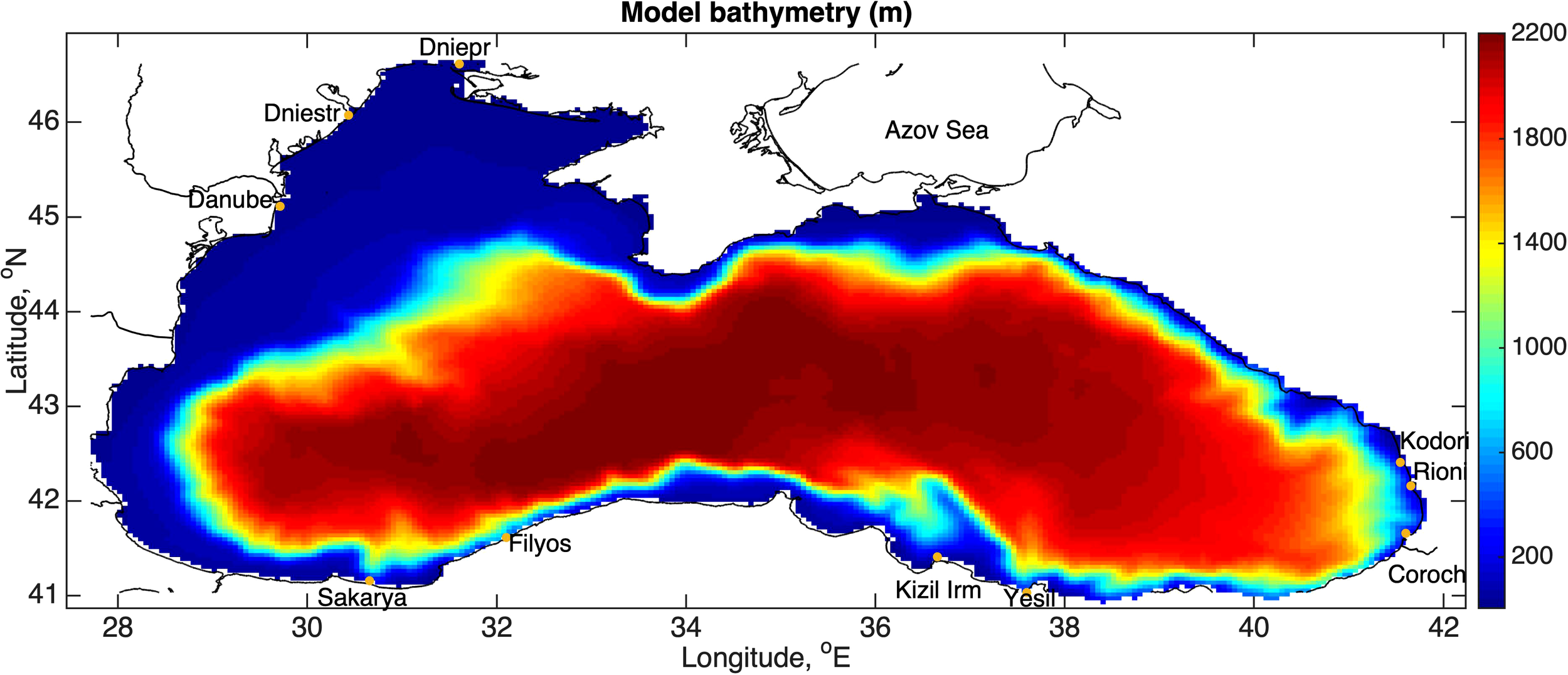
Model domain and bathymetry (m). Major rivers are also indicated.
The BS is surrounded by developed countries with flourishing agricultural production, organized fishing activity and commerce, most of which is conducted by sea. During the past decades, these anthropogenic activities resulted in vast changes of the pelagic ecosystem. For example, the increase of agricultural production and the consequent increase of nitrogen and phosphate from fertilizer use during the 80s, resulted in a significant increase of river nutrient inputs, leading to a shift in primary production, which transformed the ecosystem from mesotrophic to eutrophic (Yunev et al., 2005). Moreover, overfishing during the 80s led to the degradation of commercially exploited fish stocks (Daskalov, 2002), while the invasion, with shipping activity, of non-native species, such as Mnemiopsis leidyi (Kideys et al., 2005) had adverse effects to a number of native species like the small pelagic fish.
Anchovy (EngraulisEncrasicolus) and sprat (SprattusSpratus) are considered among the most ecologically and economically important species in the BS, due to their role in the food chain, acting as a link between the zooplanktonic production and predators like bluefish, whiting and mackerel, as well as due to their commercial exploitation (Oguz et al., 2008), being the main target of the fishing activity in the area.
The species stocks have undergone a series of fluctuations associated with changes in the BS ecosystem. Timely these coincide with the ecosystem shifts already described. More specifically, between 1960 and 1980, a significant increase in both species stocks and especially that of anchovy occurred (Oguz et al., 2012). This has been attributed to eutrophication, from the increase of river nutrient inputs (Arashkevich et al., 2014), combined with the decreasing stocks of larger fish, predating on anchovy/sprat, due to overfishing (Daskalov, 2002). Subsequently, the significant increase of fishing pressure during the 80’s, along with the negative impact of Mnemiopsis, competing for mesozooplankton and preying on fish eggs, resulted in the collapse of anchovy and sprat biomasses (Oguz et al., 2008).
After 1990, European Union regulations on waste water treatment and nutrient pollution (Vigiak et al., 2023), together with the collapse of centrally-planned economies, led to a decline of anthropogenic nutrients supply from the rivers (BSC, 2008). The relatively lower fishing activity and the control of Mnemiopsis populations from another gelatinous species (Beroe Ovata) contributed to the partial recovery of anchovy and sprat stocks during the following period (Barange et al., 2009).
The Black Sea anchovy is divided into two sub-species, the EngraulisEncrasicolusmaeticus and the species that this study focuses on, EngraulisEncrasicolusponticus. The first is only found within the Azov Sea, while the second, known as the Black Sea anchovy, occupies, as a spawning and feeding habitat, the northwestern coast of the BS (Guraslan et al., 2017) during most of the year. Anchovy spawns during summer, from June to September (Oguz et al., 2008), in the surface layer of warm and stratified areas of the west and northwestern shelf (Barange et al., 2009). The spawning area coincides with the Danube River plume zone (Bakun, 1996), a large stratified and nutrient-rich sea area that is formed due to river discharge.
The anchovy stock variability is affected by river nutrient inputs, through the subsequent changes in productivity (Daskalov, 1999). The timing of spawning can be associated with sea surface temperature (SST), which affects the metabolism, the conditioning, as well as the migration period (Hidalgo et al., 2018). During winter, it is reported to migrate to the NE coast of Turkey, where it is subjected to industrial fishery (Gücü et al., 2017). Adult anchovy may reach up to 18-20cm and has a lifespan up to 4 years (Sağlam and Sağlam, 2013).
Sprat is a small pelagic fish distributed in the whole BS, but is more abundant in the northwestern part of the basin (Daskalov and Shlyakhov, 2008). It spawns during the entire year, but with a maximum between November and March (Checkley et al., 2009). Sprat eggs are mainly found off-shore from the shelf edge and close to the main cyclonic formations (Barange et al., 2009). Sprat reaches a length of about 10 cm (Kasapoğlu, 2018) and has a lifespan of about 4 years.
Currently anchovy and sprat populations are subjected to a combination of pressures including extensive fishing activity on the two species as well as their predators (FAO, 2022), a changing climate (Hidalgo et al., 2018), alterations in river nutrients loading (Strokal and Kroeze, 2012) and the impact from invasive species (Shalovenkov, 2019). Therefore a series of key questions arise on the species stocks evolution.
Previous modeling studies of the small pelagic fish in the BS include one dimensional individual based model applications (Oguz et al., 2008; Güraslan et al., 2014), connecting anchovy biomass variability with gelatinous species and climate change respectively, as well as with overwintering migration, using a Lagrangian transport individual based model (Guraslan et al., 2017). Multi-species food web models have been also used to replicate past regime shifts and to predict the effects of future climatic conditions on the species. These either include BS-specific species food web models (Akoglu, 2023; Salihoglu et al., 2017, Serpetti et al., 2025), or Pan-European models including the BS (Schickele et al., 2021). In general, food-web models tend to include more species and analyze their interactions by describing ecosystem dynamics, towards predicting possible future changes. On the downside, the environmental conditions do not explicitly affect the higher trophic level species, instead they implicitly propagate through the lower trophic chain. Thus, food web models do not simulate fish dynamics (i.e. growth), contrary to the bioenergetic models.
In our case, a 3-D individual based model for two different species of small pelagic fish, anchovy and sprat, two-way coupled to a hydrodynamic/biogeochemical model has been developed for the BS. To our knowledge this is the first three-dimensional high trophic level model applied in the region for the aforementioned species. A long-term (1960-2020) hindcast simulation was performed to gain a better understanding on the inter-annual variability of the two species stocks. Additional sensitivity simulations were performed to investigate the role of important factors, such as fishing pressure (Daskalov, 2002) and climate change (Güraslan et al., 2014 & 2017) that may determine the species stock’s future condition. Of additional interest was the potential interaction between the two species (e.g. resource competition).
2 Materials and methods
2.1 Low trophic level model
A 3-D coupled hydrodynamic/biogeochemical model, based on POM (Blumberg and Mellor, 1983) and ERSEM (Baretta et al., 1995), has been setup for the Black Sea. Both models have been applied in the past in the Black Sea (Oguz and Malanotte-Rizzoli, 1996, Kourafalou et al., 2004). The biogeochemical model follows a functional group approach, with the pelagic food web including four phytoplankton groups (diatoms, dinoflagellates, nano- and picophytoplankton), three zooplankton groups (nanoflagellates, microzooplankton, mesozooplankton) and bacteria. The model parameterization has been customized from its implementation in the Mediterranean (Kalaroni et al., 2020a, b). Two additional functional groups, representing gelatinous omnivores (e.g. Noctiluca scintillans) and gelatinous carnivores (e.g. Aurelia aurita/Mnemiopsisleidyi) in the Black Sea ecosystem, have been also parameterized in the model, following existing modelling studies (Lancelot et al., 2002; Grégoire et al., 2008; Oguz et al., 2008). In particular, the gelatinous groups ingestion was assumed to increase linearly with prey concentration (no satiation), while mortality was assumed to decrease with temperature to account for low growth/survival during winter low temperatures, (e.g. Oguz et al., 2008; Kremer, 1994).
Moreover, a simplified parameterization of redox processes was adopted, following Oguz et al. (2014), to properly simulate the vertical variability of dissolved inorganic nutrients, oxygen and hydrogen sulphide. Other modifications in the model parameterization were mainly related with the background light attenuation coefficient, the food web matrix and nitrification (see Supplementary Tables S1–5 in supplementary material). Given the simplified parameterization of redox/anammox reactions and to prevent from a systematic model drift in the long-term simulations, the concentrations of ammonium, phosphates and hydrogen sulphide were restored to their initial fields in the deep anoxic layer by applying (on each time step) a weak relaxation (timescale:1 year), with a depth dependent function. The benthic-pelagic coupling is described by a simple first-order “benthic return” module that describes the diffusional nutrient fluxes out of the sediment, resulted from the remineralization of deposited organic matter in the sediment. The initial fields for dissolved inorganic nutrients, dissolved oxygen and hydrogen sulphide were obtained from Fichaut et al. (2003) climatology.
2.2 Fish model
A three-dimensional Individual Based Model (IBM), based on that for anchovy and sardine for the North Aegean Sea (Gkanasos et al., 2021), has been developed to simulate the full life cycle of anchovy and sprat, their spatial distribution and their most important energetic features. The model is two-way coupled with ERSEM, thus the plankton biomass consumed by the fish is removed in the biogeochemical model (Figure 2).
Figure 2
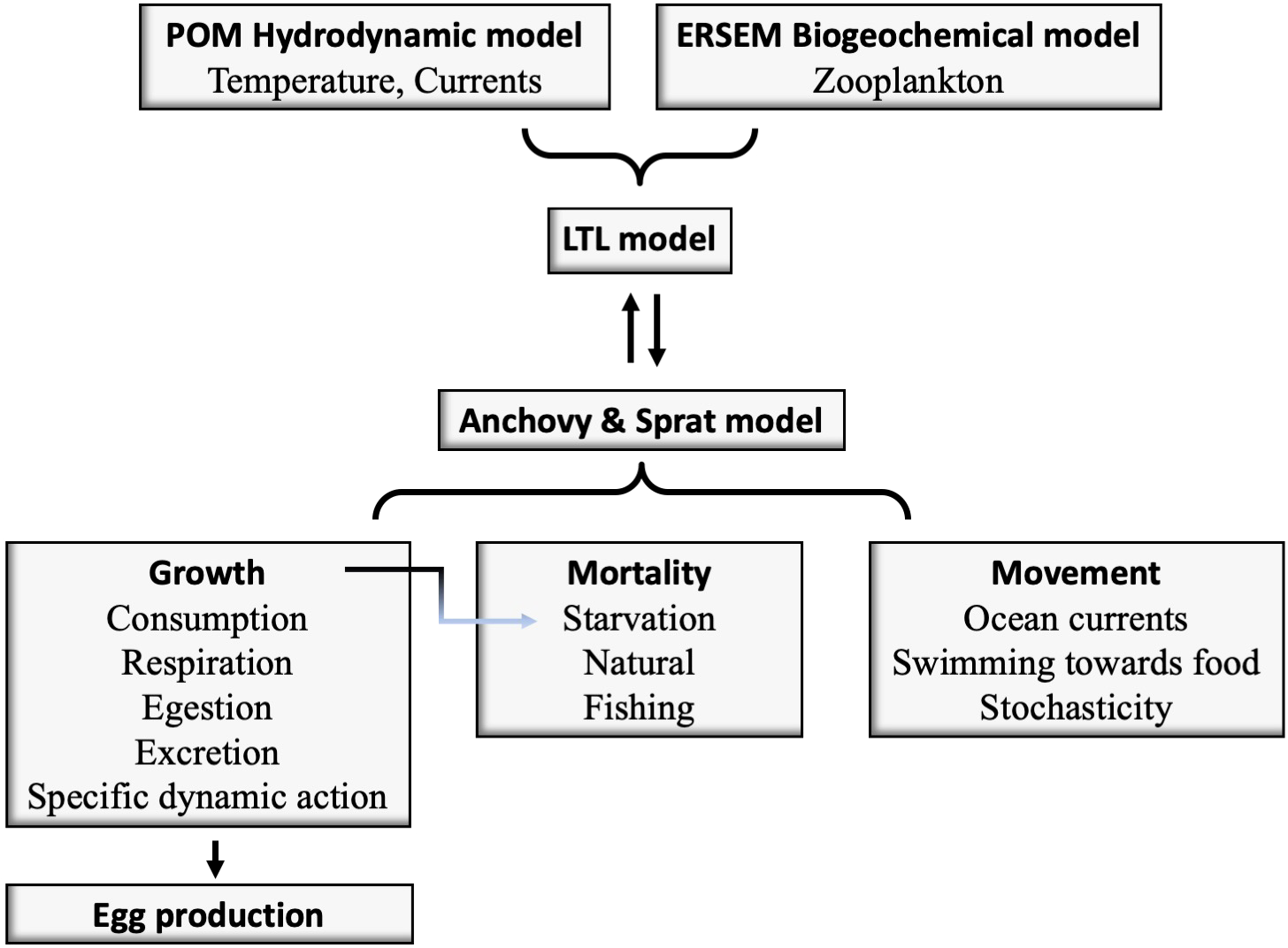
Structural diagram of the two-way coupled biogeochemical (POM-ERSEM) and small pelagic fish models.
Fish growth (WSI = fish wet weight (g)) is calculated using a Wisconsin-type bioenergetic model (Equation 1), that describes the main physiological processes like consumption (C), respiration (R), egestion (EG), specific dynamic action (SDA), excretion (EX) and the energy allocated for reproduction (Ebuffer) (Gkanasos et al., 2019; Politikos et al., 2015; Politikos et al, 2011). All components of the energy budget are in units of (g zooplankton g fish-1 day-1), converted to (g prey g fish-1 day-1). CALz and CALf stand for the caloric equivalent of zooplankton and fish respectively (Table 1).
Table 1
| Energy process | Equations | Parameters anchovy | Parameters sprat |
|---|---|---|---|
| Maximum Consumption (Cmax) |
ac = Intercept for consumption bc= Exponent for consumption W = Fish weight T = Water temperature fc(T) = temperature-dependent function for consumption |
ac = 0.41 bc= 0.31 |
≡ ≡ |
| Temperature function (Auxiliary terms) |
Qc = Slope for temperature dependence Topt =Optimum Temperature (oC) Tmax = Maximum Temperature (oC) |
Qc = 2.2 Topt=19.7a,18.76b,14.8c,d Tmax = 27 |
≡ Topt=11.7a,b,14.8c,d ≡ |
| Consumption (C) (g zooplankton g fish-1 day-1 ) |
PDj,I = density of prey type i (i = 1 corresponds to microzooplankton and i =2 to mesozooplankton) (g-prey m-3) for life stage/age class j vj,I = vulnerability of prey type i to life stage/age class j (dimensionless) kj,i = half saturation function (g-prey m-3) for life stage j feeding on prey type i. |
v2,1 = 1.0 v3,1 = 1.0 v4-8,1 = 0 v2,2 = 0.0 v3,2 = 0.0 v4,2 = v5,2 = v6,2 = v7,2 = v8,2 = 1.0 Calibrated |
≡ v3,1 = 0.5 ≡ ≡ v3,2 = 0.5 ≡ ≡ ≡ |
| Respiration (R) (g zooplankton g fish-1 day-1 ) |
A= Respiration due to swimming U = Swimming speed (cm s-1) ar = Intercept for respiration br = Exponent for respiration Q10 = Temperature dependence parameter Tm = Mean annual temperature dr = Coefficient for R for swimming speed aA = Intercept U (< 12.0oC) aA= Intercept U (≥12.0oC) aA = Intercept U (≥12.0oC) (during low feeding activity) bA = Coefficient U for weight cA = Coefficient U vs. temperature(< 12.0oC) cA = Coefficient U vs. temperature(≥12:0oC) |
ar= 0.003 br= 0.34 Q10 = 1.3 Tm =16a,b,c,d dr = 0.022 aA = 2.0 (U< 12.0 oC) aA= 12.25a,b, 11.98c, 14.21d (U≥12.0 oC) aA = 9.97c (U≥12.0 oC during low feeding activity) bA = 0.27a,b, 0.33c, 0.27d cA = 0.149 (U< 12.0 oC) cA = 0.0 (U≥12:0 oC) |
≡ ≡ ≡ ≡ ≡ ≡ ≡ ≡ ≡ ≡ ≡ ≡ |
| Egestion (EG) (g zooplankton g fish-1 day-1 ) |
af = Proportion of food egested |
af= 0.15a,b, 0.126c,d | ≡ |
| Excretion (EX) (g zooplankton g fish-1 day-1) |
ae = Excretion coefficient be = Proportion of food excreted |
ae = 0.41 be = 0.01 |
≡ ≡ |
| Specific Dynamic Action (SDA) (g zooplankton g fish-1 day-1) |
asda= Specific dynamic action coefficient |
asda= 0.10 | ≡ |
| CALz CALf |
Caloric equivalent of zooplankton (J g zooplankton-1) Caloric equivalent of fish (J g fish-1 ). |
2,580 J g zooplankton-1 3120, length <40 mm 3520, 40 < length < 60 mm 4048, 60 < length < 90 mm 5150, length > 90 mm |
≡ ≡ ≡ ≡ ≡ |
| Length-weight relationship |
y=bo+b1x+b2(x-d1)(x>d1)+b3(x-d2)(x>d2)
y, x (log-transformed fish wet weight and length) bo= y-intercept b1= slope of the function for the larval stage b2 = slope change for the juvenile stage d1 = slope change inflexion point b3 = subsequent slope change for the adult stage d2 = corresponding length for this slope respectively |
bo = -6.3 b1 = 3.49 b2 = -0.1 d1 =2.6 b3 = 0.03 d2 = 1.954 |
bo = -9.26 b1 = 5.38 b2 = -2.281 d1 = 1.699 b3 = 0.106 d2 = 2.02 |
| Max. length (mm): | Early larvae Late larvae Juvenile ( Length at maturity) |
i10 i25 i60 |
ii20 ii30 iii55 |
| Spawning period SST threshold | Start: End: |
iSST>16oC October |
ivSST<15.4oC March |
| Natural mortalities (d-1) |
i0.65, embryos i0.3, early larvae i0.1, late larvae 0.0165, juv (Calibr.) iii0.0022, age 0 iii0.0015, age 1 iii0.0013, age 2 iii0.0013, age 3 |
≡ ≡ ≡ 0.03, juv (Calibr.) iii0.0026, ages0-3 |
|
| Half saturation parameters (g prey m-3) | 0.12, earl. larv. 0.12, late larv. 0.35, juv. 0.375, age 0 0.29, age 1 0.275, age 2 0.37, age 3 |
0.12, earl. larv. 0.15, late larv. 0.37, juv. 0.42, age 0 0.33, age 1 0.28, age 2 0.335, age 3 |
|
| Egg stage (j = 1). aEarly larval stage (j = 2). b Late larval stage (j = 3). c Juvenile stage (j = 4). d Adult age-classes (j = 5-8) |
i
Oguz et al. (2008)
ii Günther et al. (2012) iiiGFCM (2014) ivBarangé et al. (2009) |
||
Anchovy and sprat model equations and parameters.
Wisconsin type models offer species specific calibration and are well established (Kitchell et al., 1997), widely used bioenergetic models for the study of marine ecosystems (Troia and Perkin, 2022). Fish populations are divided into Super Individuals (SIs) for computational efficiency, with each SI consisting of individuals of the same species, sharing common properties. Thus, SIs that belong in the same life stage or age class, have identical characteristics in terms of feeding preferences, mortalities and movement (Gkanasos et al., 2021).
Eggs and early larvae are treated in the model as neutrally buoyant particles with no active movement (Huret et al., 2010), assuming they remain in the upper 30m of the water column and their horizontal movement is only regulated by the hydrodynamic circulation. All the remaining stages perform diurnal vertical migration between the upper 30m of the surface layer and the sub-surface layer (~90m), during the night and day respectively. Horizontally, fish move towards areas with higher food concentration, with maximum velocity being proportional to their body length, while a random movement factor and a bathymetry check function are also adopted (Politikos et al., 2015).
In the model, three types of mortality regulate the species population: natural, starvation and fishing mortality. The natural mortality values for the anchovy early stages (eggs, larvae) were obtained from Oguz et al. (2008), and in the absence of other available data, applied to sprat early stages as well. The corresponding values for the juvenile stages have been calibrated (due to the lack of data) and are different for anchovy and sprat (Table 1), while those for both species adult stages were obtained from the GFCM (2014) report for the BS (Table 1). Starvation mortality is also included in the model, with individuals removed from the population once they experience a 30% weight loss (Gkanasos et al., 2019). Finally, fishing effort on the species stocks is represented through an additional yearly varying fishing mortality parameter (see Model Setup section).
For the needs of the bioenergetics model setup, various parameters have been derived from the available literature and are presented in Table 1. Sprat parameters are identical to those of anchovy, except from those shown in the Table. As already mentioned, both species have a lifespan of 4 years, which is divided into 8 stages in the model: egg, early and late larval, juvenile and four adult stages.
Anchovy transitional lengths for early stages (larvae and juveniles) were based on Oguz et al. (2008). In the absence of Black Sea-specific data for sprat, larval transitional lengths are adopted from Günther et al. (2012) for North Sea sprat, while juvenile lengths were taken from the GFCM (2014) report (Table 1).
In the bioenergetic model, individuals’ weight is calculated using Equation 1., and fish length is derived from weight (Table 1), using a piece-wise length-weight relationship (Politikos et al., 2011). Finally, consumption half-saturation parameters (regulating somatic growth), are calibrated. These are stage and prey specific (Table 1), therefore a total of 14 parameters (7 for each species) are calibrated for all life stages (following egg hatch). For both species, a temperature dependent egg stage development duration is adopted in the model, following Gatti et al. (2017) formulation.
Observations on the daily evolution of larval lengths were obtained from Oguz et al. (2008) for anchovy and Günther et al. (2012) for sprat. Data of weight and length for the adult stages were obtained from Samsun (2006) and Oguz et al. (2008) for anchovy and Kasapoğlu (2018) for sprat.
The inter-annual variability of the anchovy stock over the 1960–2020 period, is reconstructed using data and model derived stock estimations from Oguz et al., 2008 for the 1960–1992 period, from GFCM (2014) from 1993 to 2013 and from Bilir (2019) and Gücü et al., 2021 for the years 2016 and 2020. For sprat, stock estimations were obtained from GFCM, 2014 for the years 1960–2013 and from Scientific, Technical and Economic Committee for Fisheries (STECF) – Black Sea assessments (STECF-15-16) (2015) for the years 2014-2017.
2.3 Model setup
We have chosen to study the 1960–2020 period, in order to be able to reproduce the ecosystem and stocks fluctuations described above, as well as their current state, while also exploiting the available data for the selected period. The atmospheric forcing used for the needs of the simulations were obtained from ECMWF – ERA5 (Hersbach et al., 2020) with 0.25° x 0.25° resolution. The river discharge and nutrient inputs were based on Ludwig et al. (2009) for the 1960–2000 period and Strokal and Kroeze (2012) for the remaining twenty years (see Supplementary Figure S.1 in supplementary material).
Yearly varying fishing mortality rates were based on currently available data (see supplementary Figure S.2). For anchovy, fishing mortality was obtained from Ivanov and Panayotova (2001) for the 1968–1988 period and from GFCM (2014) for the 1989–2013 period. For the periods before 1968 and after 2013, fishing mortality is assigned to the values of 1968 and of 2013 respectively. For sprat, fishing mortality data for the 1994 to 2013 period are obtained from GFCM (2014) and for the remaining periods, the marginal values were also used. In the model, fishing effort is uniformly applied across the BS continental shelf (maximum depth ~300m, see Supplementary Figure S.3 in supplementary material), although Turkish fisheries represent the greatest pressure on fish stocks (O’Higgins et al., 2014).
Anchovy and sprat are considered to be shelf and open sea spawners respectively (Daskalov, 1999), but their habitats largely coincide with the continental shelf (BSC, 2008; GFCM, 2014; Kaschner et al., 2019). Therefore, this area was used for the initial placing of both species super individuals in the model.
Anchovy migration patterns are referred to be primarily dictated by the cooling pattern of the surface waters (Gücü et al., 2017), as well as by the wind direction and the BS currents. In the literature, contrary to anchovy, sprat is not referred to migrate for breeding purposes. In the model, both species are directed to higher zooplanktonic concentrations, therefore the southward migration of anchovy for wintering, as described in the literature, is not explicitly parameterized.
In the reference simulation, the atmospheric forcing, river discharge, nutrients inputs and fishing mortality are inter-annually varying, as described above. In order to investigate the contribution of hydrodynamics and fishing mortality in the stocks inter-annual variability, two additional sensitivity experiments were performed, in one keeping the atmospheric forcing constant and in the other the fishing mortality. In the first experiment (perpetual, ‘perp’), the atmospheric forcing of the first year (1960) is perpetually repeated, thereby removing the effect of hydrodynamics and particularly temperature from the fish stocks interannual variability. In the second experiment (stable fishing mortality, ‘stable fmort’), the fishing mortalities remain constant at their mean values over the entire simulation period, allowing to investigate the effect of fishing effort on the stocks inter-annual variability.
For the model initialization, a number of 1000 SIs for every age class from the juvenile to the adult age-3 stage of both species (with reference weights per age), were evenly spread along the BS continental shelf. The model resolution is 1°/10 x 1°/10 and the time step is set to 800s. The simulation commenced on 1st January 1960 with assigned biomasses for the two species in accordance with their historical stock estimations.
The first twenty years of the simulation were used for the model calibration, by evaluating basic model outputs from the entire population, like the average weight, the biomass evolution, the egg production and the late larvae growth. During this process, no cost function is used, instead the model outputs are checked to lie within the data range of this period. With the completion of the simulation, model outputs are validated against available data from the literature in terms of average values or variability (R-square), for the entire simulation period.
3 Results
3.1 Reference simulation
3.1.1 Biogeochemical model
In Figure 3, the inter-annual variability of the simulated SST and mean (0-50m) concentrations of nitrates, phytoplankton and mesozooplankton, is shown in 5-year averages over the 1960–2020 period. The variability in plankton biomass is primarily controlled by river nutrient inputs, characterized by an increase over the 1970–1990 period followed by a decrease until 2000 (see supplementary Figure S.1). Afterwards and until 2020, phosphorus concentrations are increasing, since riverine inputs of dissolved inorganic phosphorus at the Southern BS are projected to rise up to 200% of the current status until 2050 (Strokal and Kroeze, 2012).
Figure 3
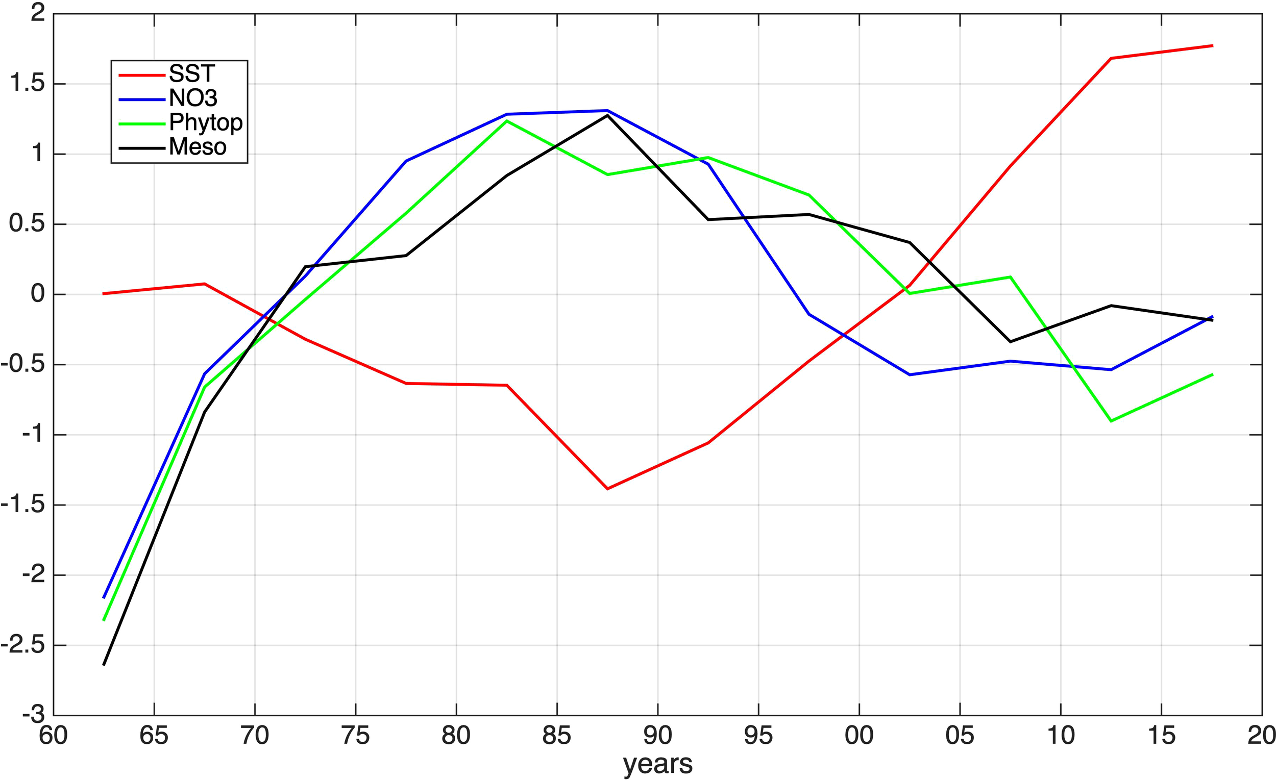
Simulated inter-annual (5-year average) anomaly (=(var-var_mean)/var_std) variability of mean nitrates (NO3, blue line), phytoplankton biomass (Phytop, green line), mesozooplankton biomass (Meso, black line) and sea surface temperature (SST, red line).
The simulated temperature shows a continuous increase (~0.056 °C/year) from 1985 onwards, which is consistent with satellite (CMEMS), SST variability (see supplementary Figure S.4). This results in an increase of stratification, which, combined with the decreasing river nutrient inputs mentioned above, leads to a decline in both phyto- and zooplankton biomass.
In Figure 4, the mean (1960-2020) spatial distribution of the SST and mesozooplankton concentration is shown. The SST distribution is characterized by an increasing gradient from the North-Western to the South-Eastern BS, showing a good agreement with available satellite data (CMEMS SST, 0.05° resolution, see supplementary Figure S.5). Mesozooplankton is more abundant in the more eutrophic North-Western BS, as a result of the nutrient inputs from surrounding rivers. A similar pattern is also simulated for Chl-a, which is also in reasonable agreement with ocean color satellite products (https://hermes.acri.fr, 0.04° resolution, see supplementary Figure S.6).
Figure 4
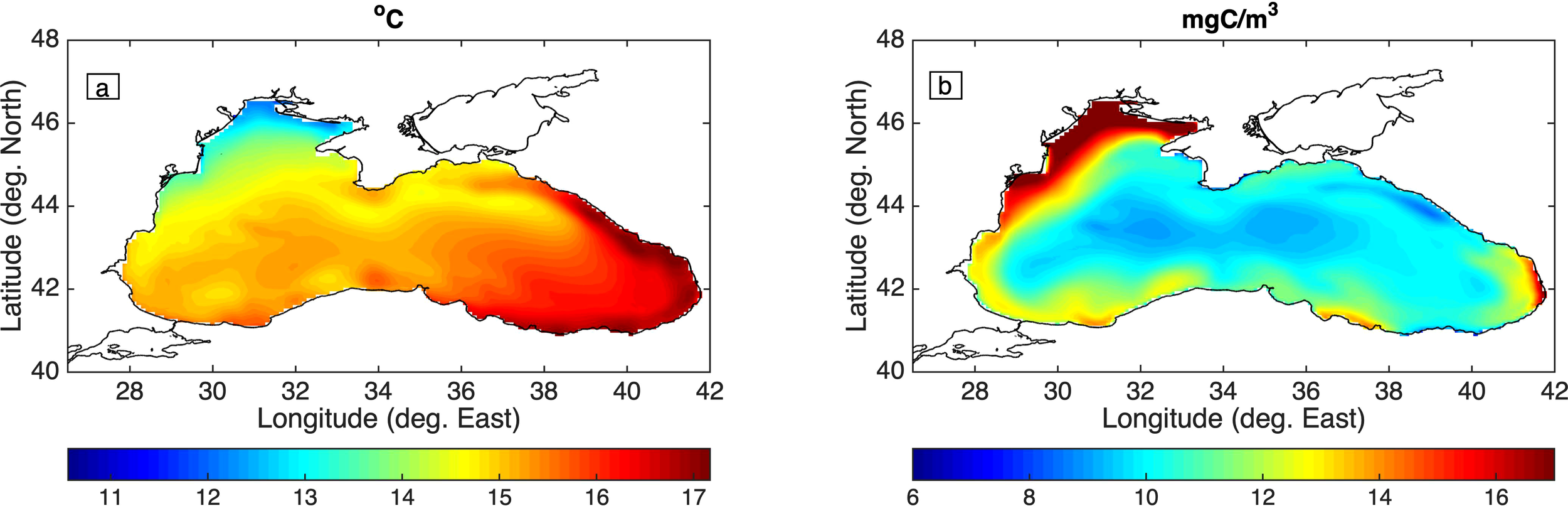
Simulated mean (1960-2020) average (a) sea surface temperature (oC) and (b) mesozooplankton (mgC/m3) concentrations.
In supplementary Figure S.7, the average simulated SSH for the 2010–2020 period, against satellite data (CMEMS Sea-level, 0.0625° resolution) is presented. The model successfully reproduces major semi-permanent circulation patterns (Staneva et al., 2001), such as the cyclonic Rim Current and major sub-basin anti-cyclonic gyres (Batumi and Sevastopol eddies), as depicted through the SSH variability.
3.1.2 Fish IBM larvae growth
In Figure 5, the mean (1960-2020) simulated daily evolution of larvae length from all SIs is shown and is validated against larvae length data from the Black Sea for anchovy (Oguz et al., 2008). For sprat, Baltic Sea larvae length data are used (Günther et al., 2012), in the absence of other available data. The modeled anchovy larvae length is found on the upper bound of the data, with a growth rate of 0.79mm day-1, while the data derived growth rate ranges from 0.53 to 0.76mm day-1. Therefore anchovy transitional length from the larval to the juvenile stage (25mm) is reached relatively faster, as compared to the data. Given that stage mortality is cumulative on a daily basis, higher growth rates result in reduced larval mortality and thus increased anchovy population as a whole. Similar to anchovy, the simulated sprat larval growth appears also relatively higher on-average (0.62mm day-1), as compared with the data (0.53 to 0.65 mm day-1). However, in this case it falls closer to the average data trajectories.
Figure 5
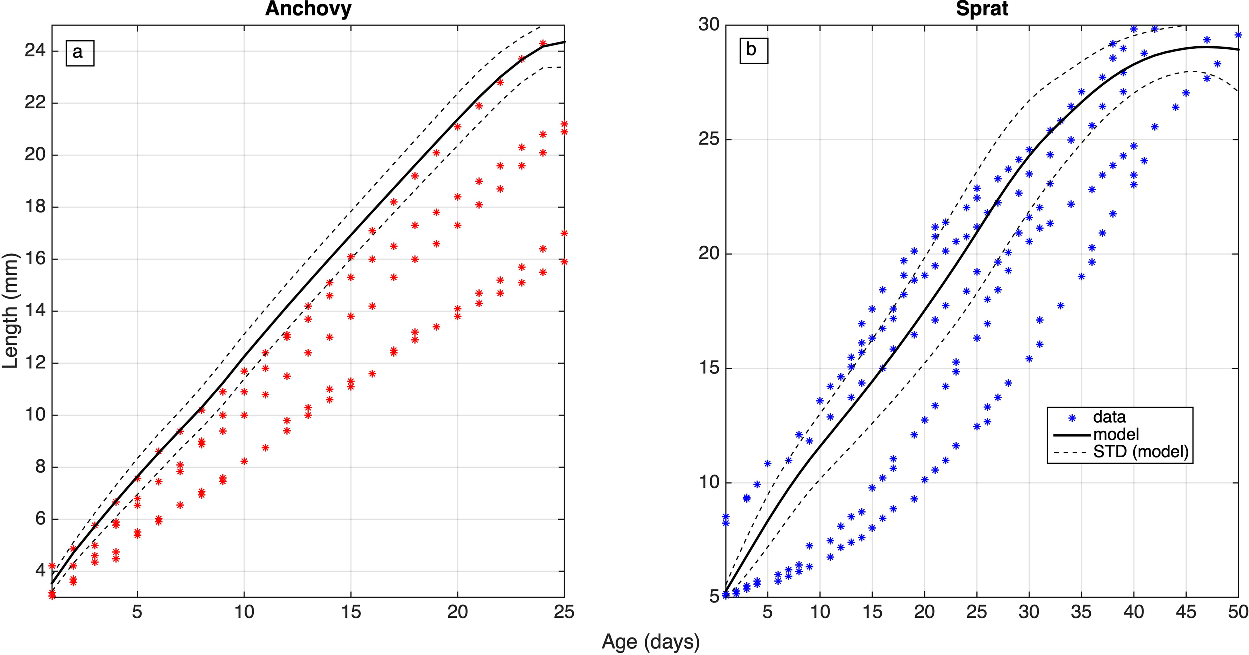
Simulated (average: black solid line, average ± STD: black dashed lines) mean (1960-2020) daily evolution of (a) anchovy and (b) sprat larval length (mm), validated against observations, obtained from Oguz et al. (2008) and Günther et al. (2012).
3.1.3 Fish IBM adults length/weight
For the post larvae stages (juveniles and adults) the data derived evolution of both species weight and length is fairly well reproduced (Figure 6), by the average simulated weight/length-at-age for the 1960–2020 period. There is a good agreement with the data for most age-classes, with the exception of anchovy age-1 and sprat age-3 weight, which appear under- and overestimated respectively.
Figure 6
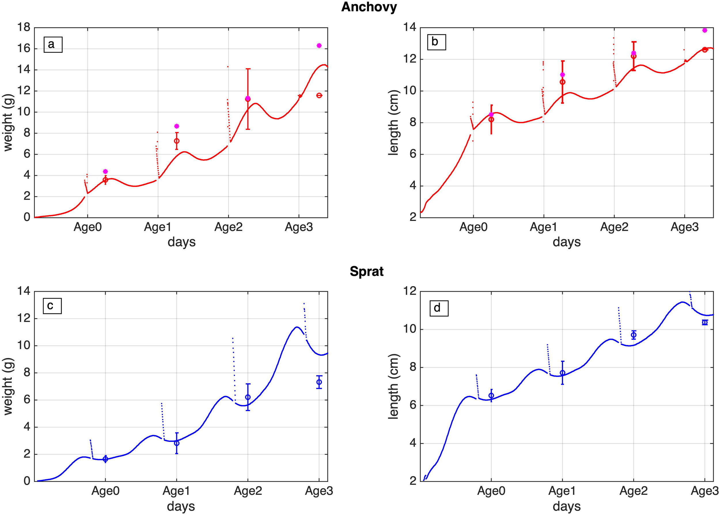
Daily evolution of anchovy (a, b) and sprat (c, d), weight (g) and length (cm) for the juvenile and adults (0-3) stages (days), against available data obtained from Samsun (2006) and Oguz et al. (2008) for anchovy and Kasapoğlu (2018) for sprat.
3.1.4 Fish IBM biomass spatial distribution
During the 60 years of the simulation, both species stocks showed a similar spatial distribution (Figure 7), with anchovy being more widespread due to the significantly higher biomass. Relatively higher stock concentrations are simulated for both species in the North Western BS shelf, followed by the South Eastern and South Western BS shelf, particularly in coastal areas, affected by river nutrient inputs, resulting in an increased plankton productivity (see Figure 4).
Figure 7
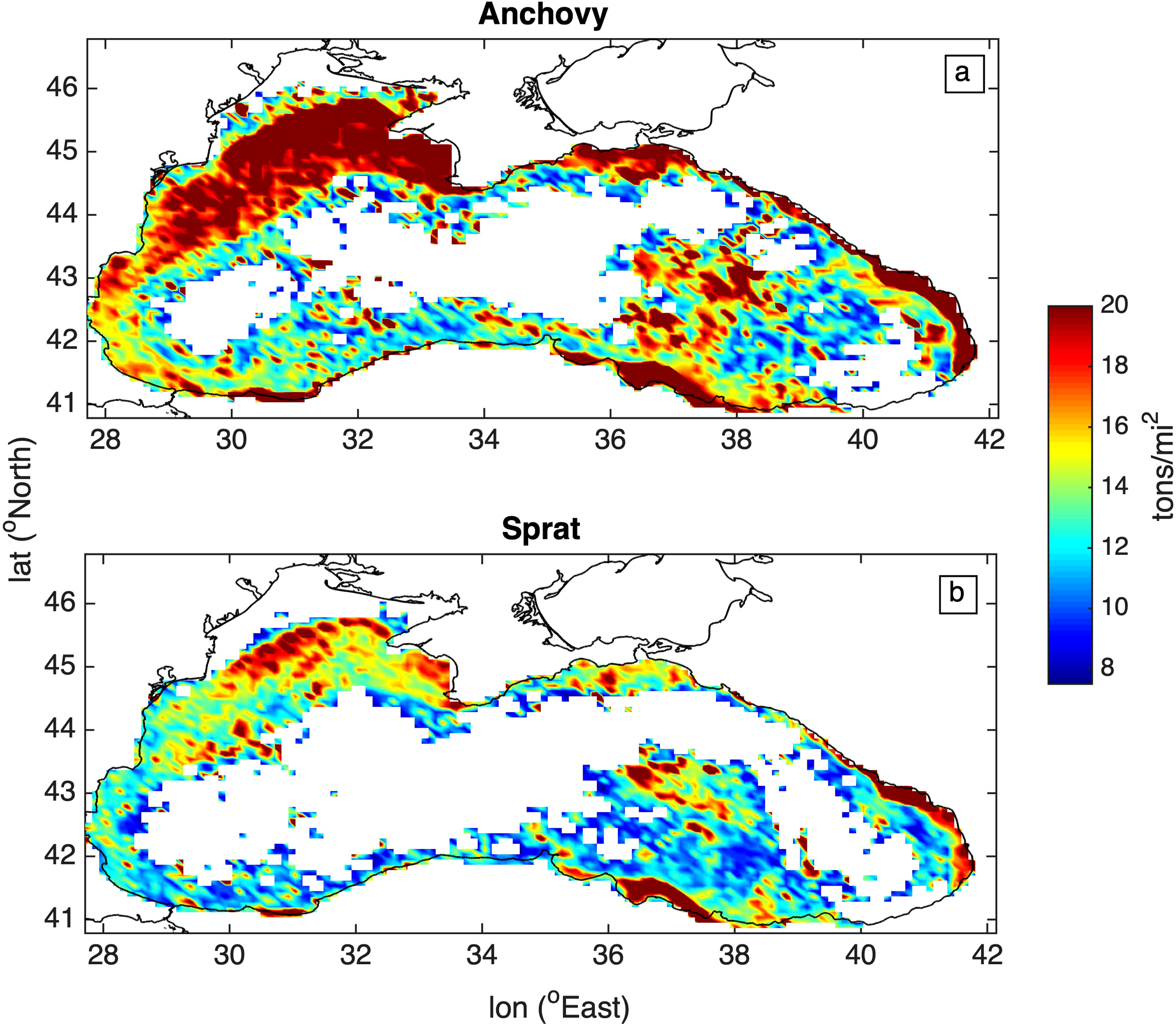
Average spatial distribution of (a) anchovy and (b) sprat stocks (tons/mi2).
Spatially, stocks deviated from the coastal stock distribution described in the literature (GFCM, 2014), in the southeastern part of the Black Sea. There, both species gradually spread in deeper areas, beyond the shelf (Figure 7), probably due to an increase of mesozooplankton in the specific area (Figure 4).
3.1.5 Fish IBM biomass inter-annual variability
One of the main goals of the present study, is the successful representation of the anchovy/sprat inter-annual stock dynamics. So despite the anchovy huge biomass data variability and the very low initial stock values, the model replicated the observations satisfactory in terms of the amount of variance (R-squared: 0.33), as shown in Figure 8. The model also reproduced the observed increase of the anchovy stock from 1960 to mid-80s, which may be attributed to the effect of increasing river nutrient inputs (see supplementary Figure S.1), resulting in an increase of plankton productivity (Figure 3), combined also with the sustainable fishing effort (supplementary Figure S.2). Another factor, discussed below, which favored this anchovy stock increase is the gradual decrease of SST until the mid-80s (Figure 3).
Figure 8
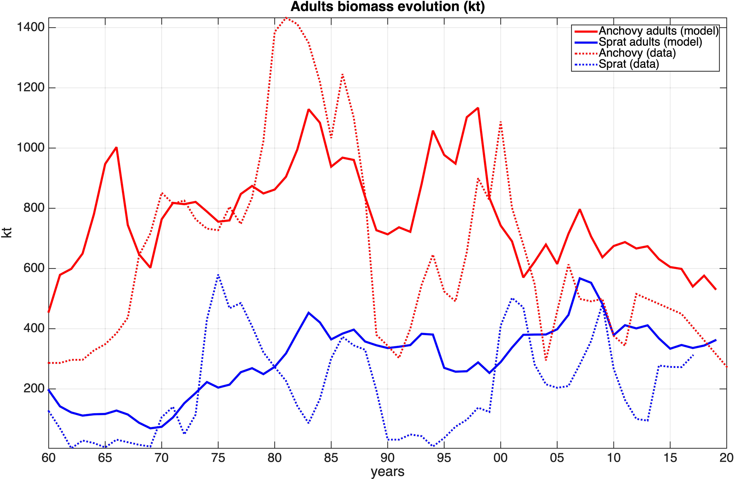
Model simulated anchovy and sprat biomass (kt) against stock estimates for the 1960–2020 period.
Between the mid-80s and mid-90s, the anchovy overexploitation (supplementary Figure S.2) led to its stock decline. In the late 90’s, a relatively lower fishing activity resulted in the anchovy stock recovery. However, after 2000, the considerable increase of the SST and the drop in nutrients concentration and consequently primary production and mesozooplankton biomass (Figure 3) caused an almost linear stock decrease.
The simulated averaged sprat biomass is close to that derived from observations, but the model failed to simulate the inter-annual variability, as successfully as it does for anchovy (R-squared: 0.14). This may be partly attributed to the lack of fishing mortality data during the 1960–1993 period. The simulated sprat biomass variability shows two peaks, one during the early 80s and one between 2000 and 2010 and both seem to be a coarse representation of the peaks displayed in the data.
The inter-annual variability of the two species stocks does not suggest the existence of density dependence, related to resource competition between them. On the contrary, the two stocks appear to be in phase, both in the model and in the data inter-annual variability, except during the 1980–1985 period, when the opposite variation observed in the data indicates asynchronous stock variability, suggesting a potential resource competition due to the excessive stock development of anchovy.
3.2 Sensitivity experiments
3.2.1 Atmospheric forcing
The role of the atmospheric forcing was further investigated by evaluating the interconnection between the SST and the species stocks. To this end, the variability of a series of parameters in the reference simulation (ref), including stage-to-stage survival rates, adult weight, egg production and biomass was examined in relation to SST variability and compared to those of a “perpetual” (perp) simulation, in which interannually non-varying atmospheric forcing (repeating 1960) was used.
The “perp” simulation SST remains higher until 2004, while during the following years the “ref” interannually varying SST increases, reaching a maximum difference of 0.75°C (Figure 9a). The SST during summer is higher in the “ref” experiment, across the entire simulation period, whereas this situation reverses during winters (not shown).
Figure 9
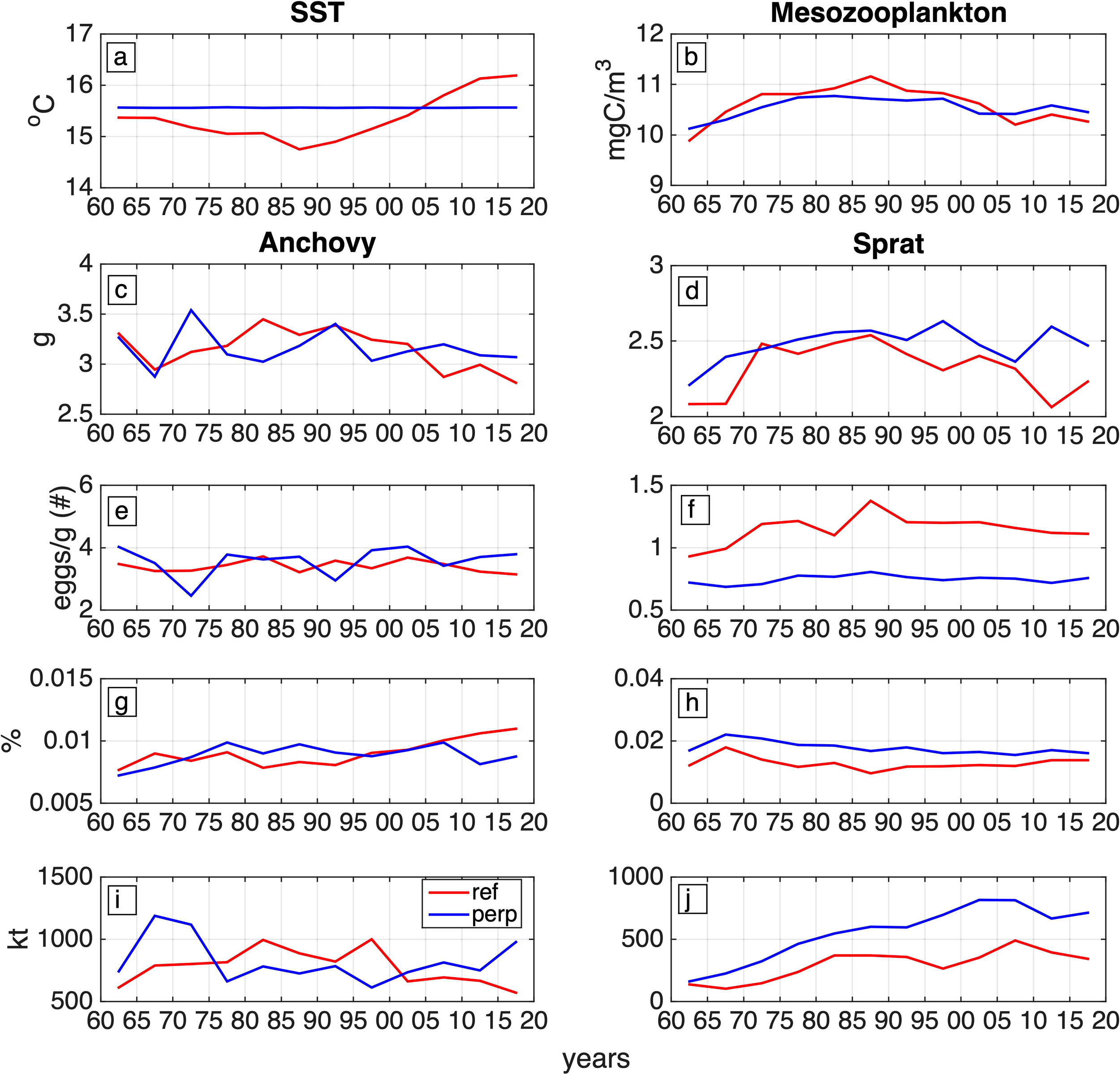
Five-year averages of (a) SST (oC), and (b) mesozooplankton concentration (mgC/m3) at the anchovy and sprat habitats (0-90m average). Anchovy and sprat five-year average of, age-1 adults wet weight (g) [panels (c, d)], normalized egg production [# eggs/g of adults wet weight, panels (e, f)], survival from egg to adult-1 stage [%, panels (g, h)] and biomass evolution [kt, panels (i, j)] from the ref (red line) and the perp (blue line) simulations.
The declining mesozooplankton concentration that may be seen after the 1980s decade in both experiments (Figure 9b), follows the reduction of river nutrient outputs, but is relatively steeper in the “ref” simulation. This is due to the effect of the SST, with the two parameters (mesozooplankton, SST) showing a statistically significant negative (r=-0.73, p<0.01) correlation (Table 2) in the “ref” simulation.
Table 2
| SST | Mesozooplankton | Egg production | ||
|---|---|---|---|---|
| -0.73, < 0.01 | ||||
| Anchovy | Weight of age 1 adults | -0.60, < 0.01 | 0.44, < 0.01 | 0.47, < 0.01 |
| Egg-early larvae survival (hatching) | 0.66, < 0.01 | |||
| Adult biomass | -0.46, < 0.01 | 0.36, < 0.01 (4yr. lag) | ||
| Sprat | Weight of age 1 adults | -0.42, 0.012 | 0.57, < 0.01 | |
| Egg-early larvae survival (hatching) | 0.54, 0.01 | |||
| Early to late larvae survival | 0.49, < 0.01 | |||
| Egg production | -0.43, 0.01 (SST winter) |
|||
Statistically significant correlation coefficients [r,p] between variables of each species and environmental variables.
Therefore, until 2005, the lower annual mean SST in the “ref” experiment leads to comparatively higher mesozooplankton concentration, while afterwards the situation reverses (Figure 9b).
The effect of temperature on the anchovy and sprat stock is first investigated in relation to the weight of age-1 adults, which represent the larger portion of the stock population, producing the largest amount of eggs.
In the “ref” simulation, the anchovy adult age-1 weight (Figure 9c), is positively correlated (Table 2) with mesozooplankton (r=0.44, p<0.01), which is expected, based on the effect of prey availability on the fish growth. It is also negatively correlated with increasing SST (r=-0.60, p<0.01), which is related to an increase in energetic needs. This is particularly apparent after 1980 and leads into a somatic condition degradation.
The weight of anchovy age-1 adults is also directly related to egg production, showing an important correlation (r=0.47, p<0.01), which leads into a spawning restriction, especially during the post 2000 period (Figure 9e). The above condition is not obvious in the “perp” simulation (beyond the intermediate fluctuations due to model dynamics), since the temperature is stable and the anchovy adults energetic needs do not increase.
As can be seen in Table 2, the sprat adult-1 weight in the “ref” simulation (Figure 9d), is also positively correlated to mesozooplankton (r=0.57, p<0.01) and negatively to SST (r=-0.42, p=0.012), but unlike anchovy, it is not correlated with egg production. Spawning is negatively impacted only by the winter SST (r=-0.43, p=0.01), therefore the lower winter SST in the “ref” simulation (not shown), subsequently leads to a higher sprat productivity across the entire 1960–2020 period (Figure 9f).
Therefore another factor that regulates the stock population, the survival from the egg to the adults stage was investigated. Considering that eggs hatch faster at higher temperatures (Gatti et al., 2017), the egg survival for both species is positively correlated with SST (anchovy: r=0.66, p<0.01, sprat: r=0.54, p<0.01, Table 2), as egg mortality is applied for a relatively shorter stage duration.
Beyond this intermediate stage, no clear connection between different stages survival and biomass inter-annual variability was found for anchovy, although as can be seen in Figure 9g, the overall egg to adult 1 survival seems to follow an opposite pattern as compared to the anchovy biomass.
On the other hand, an important correlation was found between SST and sprat early to late larval survival (r=0.49, p<0.01, Table 2). In total, egg to adult 1 survival was magnified from the higher SST during the first 45 years of the “perp” simulation (Figure 9h) and then reduced following the SST inversion among the two simulations. A small but noticeable (2.36%) increase in the late larvae growth rate in the “perp” simulation may also had a synergetic effect in the egg to adult survival rise.
The above findings suggest that species biomasses are expected to evolve in different ways. Anchovy biomass in the “ref” simulation, being anti-correlated with SST (r=-0.46, p<0.01), evolves inversely to that (Figure 9i). In the “perp” simulation, the anchovy stock, after a steep increase (probably due to population dynamics), follows a biomass correction and after that, a near-linear stock increase, probably ought to the elevated average (1960-2020) late larval growth as discussed before (Figure 5).
Moreover, the anchovy stock in the “ref” simulation is positively correlated to the normalized egg production (r=0.36, p<0.01) with a 4-year lag, which in turn is connected to the adults weight and especially that of age 1 (r=0.47, p<0.01).
Therefore, the atmospheric forcing plays a crucial role in the anchovy adults, not only through food provision, but also because of its impact in bioenergetic functions, such as respiration. This has direct consequences in the fecundity, that in the case of anchovy determines the condition of the stock.
The sprat stock is calibrated to simulate the overall upward trend that appears in the data, (Figure 9j), therefore an increasing trend is present in both experiments. Especially in the “perp” experiment, the higher SST throughout the first 45 years of this simulation results into elevated survival from the egg to the adult stage and thus a stock escalation.
3.2.2 Fishing mortality
Along with the reference simulation, an additional simulation was performed to investigate the impact of the fishing mortality. In this simulation (stable fmort), the fishing mortality of both species does not vary interannually, but instead remains stable throughout the entire simulation period, using their average 1960–2020 value. The impact of fishing mortality is then evaluated, taking the difference of anchovy/sprat biomass between the two simulations.
As shown in Figure 10, there is a statistically significant negative correlation between the differences in fishing mortality and species biomass (r=-.66, p<.01 and r=-.68, p<.01 for anchovy and sprat respectively). For anchovy this effect is particularly noticeable during the 1960-1974, 1985–1990 and 2000–2012 periods. The lower (by ~51%) fishing mortality during 1960–1974 results in a significant increase (up to ~250kt) of the anchovy stock. Similarly, the increase in fishing pressure (+67% and +30%) during 1985–1990 and 2000-2012, results in a decrease of the anchovy stock by 235kt and 255kt respectively. During the remaining years, steep variations in fishing mortality and fish model dynamics, result in less distinct stock fluctuations.
Figure 10
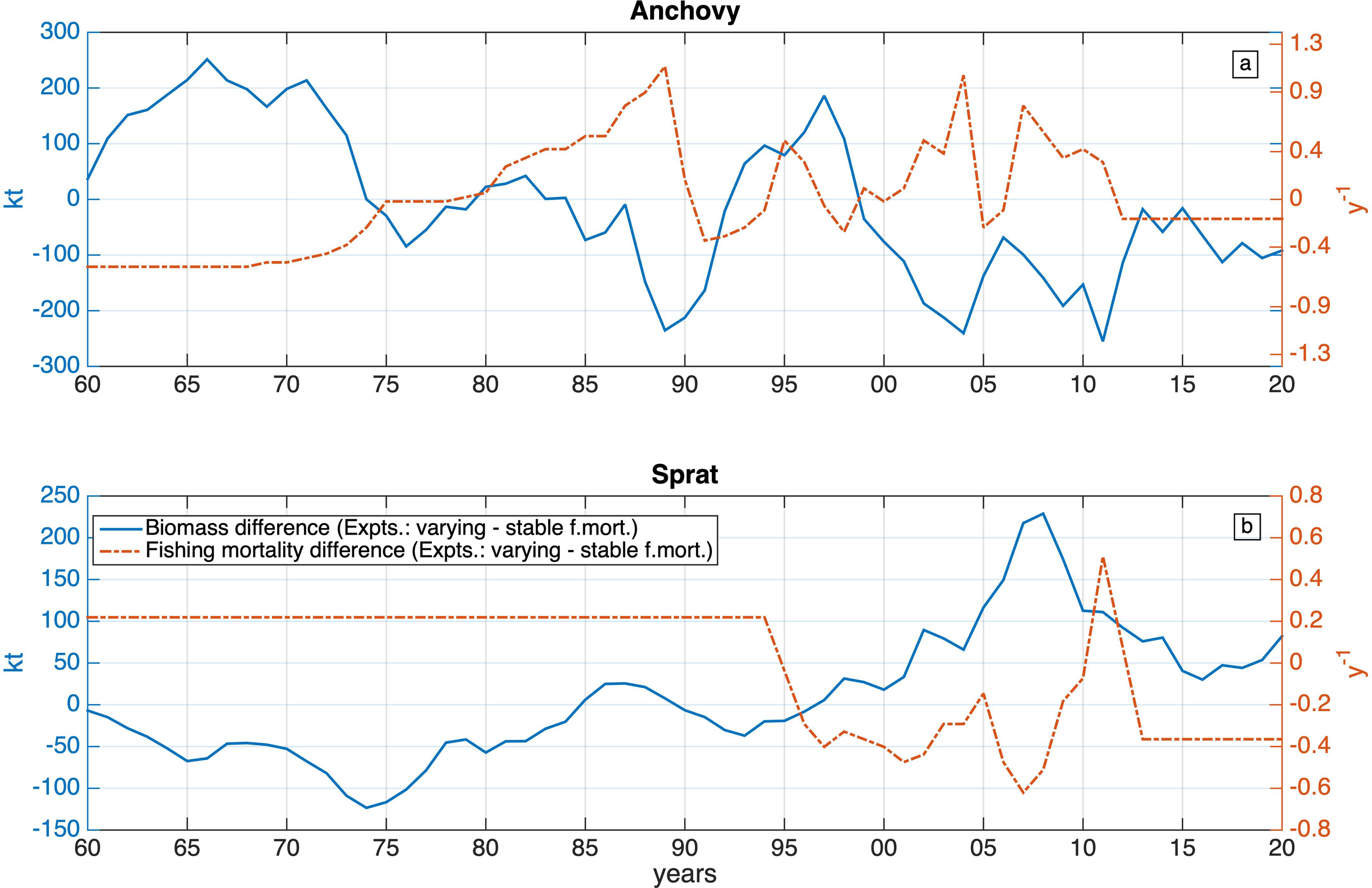
Anchovy (a) and sprat (b) differences among fishing mortality (right axis, y-1) and biomass (left axis, kt), between the experiments with varying and stable fishing mortality (varying - stable fmort).
Unlike anchovy, the sprat stock difference is more stable due to the constant fishing mortality applied between 1960 and 1994, as well as due to the generally lower fishing mortality (as compared with anchovy), during most of the remaining period. The relatively higher fishing mortality (+22%) during 1960-1994 (as compared with the mean 1960-2020) results in a decrease (123kt) of the sprat stock. Similarly, the relatively lower fishing mortality during almost the entire remaining period, is followed by an increase of the sprat stock by 229kt.
The maximum anchovy fishing mortality rate difference of 1.1 yr-1, leads to a stock difference of -251kt, while sprat maximum stock difference of 228kt occurs following a mortality rate difference of up to -0.6 yr-1. This is because anchovy stock shows greater tolerance to harvesting, due to its significantly larger size, as compared to sprat.
It should be noted that in both experiments, the average biomass over the entire simulation period remains the same. Despite their sensitivity to external pressures due to their short life cycle (Gkanasos et al., 2021), both anchovy and sprat stocks retain the ability to recover. Thus, the effects of overfishing during a certain period, can be reversed by reducing fishing effort, provided that stock levels remain above a collapse threshold.
4 Discussion
During the 1960–2020 period, SST in the BS significantly increased by almost 1.5°C. This temperature increase was combined with a decrease in nutrients supply from rivers after the 1990s. Projections (2000-2050) report that nitrate (DIN) concentrations in the BS will keep on decreasing, while phosphate (DIP) concentrations will most probably increase, due to high sewage inputs in the Southern BS (Strokal and Kroeze, 2012).
As a result, the primary production has been decreasing since 1990, favored by increasing water column stratification, which hinders the upward transport of nutrients to the surface (Salihoglu et al., 2017) and is expected to intensify as a result of the climate change.
Small pelagic fish populations have also undergone significant fluctuations, mainly due to anthropogenic factors, such as commercial exploitation. For example, the increase in anchovy biomass during the 70s, led to a peak in exploitation, resulting to its stock collapse by the end of the 80s (Barange et al., 2009).
In this study, the main drivers affecting anchovy and sprat were parameterized and incorporated in the model. These include anthropogenic pressures, such as river nutrient inputs and fishing pressure, as well as key environmental changes.
Model results capture the growth of the two species from larval to adult stages and their inter-annual biomass variability. Simulations show that the anchovy stock variability is more accurately described in the model, compared to the data, in relation to that of sprat. Although no resources competition between the two species emerges, within a certain stock range (close to the observed values), we consider possible that the species with the most limited stock is affected by the stock variability of the dominant species (in terms of stock size).
Furthermore, the limited historical fishing effort data availability for the pre 1975 and post 2013 period, combined with the large stock variability due to the very low values over the ‘60 and ‘90 decades, introduce further uncertainties and make the accurate stock representation a very challenging task.
The spatial distribution of both species stocks covers the BS continental shelf, with peaks in the Northwestern and Southeastern regions. The significantly larger anchovy stock imposes wider space occupation across the BS, as compared with sprat, a pattern consistent with what is documented for most areas inhabited by antagonistic small pelagics (Barange et al., 2009).
The BS anchovy stock appears to be negatively affected by a temperature increase, a condition similar to the small pelagics state in other regions of the world (Lluch-Belda et al., 1992; Taboada et al., 2023; Menu et al., 2023). This negative effect of temperature is partly related to decreasing mesozooplankton abundance due to increasing stratification, but is also related to increased energetic needs of anchovy adults, which results in a decrease of their weight and egg production. The above outweigh the positive impact of the rising temperature on the hatching of anchovy eggs.
Thus, after the 1990s, the reduction in river nutrients inputs, combined with an escalating temperature, resulted in a decrease in food availability and a rise in anchovy adults’ energetic needs, resulting in weight reduction, on which egg production depends. This effect is more apparent in the adult stage of age one, as they play a dominant role in stock recruitment. It is an immediate consequence of climatic change, causing an increasing divergence between SST and the species’ optimal consumption temperature. This parameter plays a crucial role in the development of the individuals, by regulating the basic energy requirements depending on the prevailing temperature. Therefore fluctuations around the reference values may cause significant growth, reproductive and thus population alterations, especially in long-term climatic simulations.
In general, the reaction of anchovy stocks to climate change is reported to be habitat specific, since each stock is affected differently. This results from the stocks different reaction to changes in a series of environmental factors like the extension of spawning areas, trophodynamic alterations and recruitment variability (Peck et al., 2013 and references therein).
The sprat stock follows a positive bias in both the reference and the perpetual simulation with non-varying atmospheric forcing, in agreement with the overall sprat stock data trend. This stock rise is more apparent in the perpetual simulation, due to the positive correlation between survival of both the initial stages and overall, with temperature. Similar to the BS, the Baltic Sea sprat stock during the 1990–2000 period, was also significantly developed and findings indicate (Köster et al., 2003) that it was similarly affected by the climatic change, owing to the same mechanism described above.
The negative connection between egg productivity and the winter SST implies that the lower average winter temperatures in the “ref” simulation, resulting from the wider colder regions, are more suitable for sprat spawning (Lima et al., 2022). This finding aligns with the wintering behavior of sprat in the North and its nonmigratory spawning strategy, unlike anchovy. This finding, once again highlights the potentially contradictory contribution between a series of parameters that regulate the condition of a species (Peck et al., 2013). In general, it is expected that small pelagics stocks, especially at the latitudinal limit of their distribution, will face the most distinct changes (Rijnsdorp et al., 2009).
As already stated, throughout the simulation period, the SST during summer months was higher in the “ref” simulation, contrary to the winter SST, being higher throughout the “perp” simulation. This attributed to faster growth, therefore reduced cumulative mortality of the early larvae during the corresponding periods. Thus the percentage of anchovy and sprat early larvae that evolved to the late larval stage (survival) was greater in the “ref” and “perp” simulations respectively. This finding is not depicted in the overall (egg to adult) survival of anchovy, while in sprat it can partly explain the notable stock difference among the “ref” and “perp” simulations.
Overall, it appears that while anchovy and sprat stocks fluctuated almost in parallel in the past, after 2000 the reduction of resources (Figure 3), combined with rising temperatures have intensified their biological differences and may have created conditions of competition between them. Asynchronous stock variability among small pelagics is reported to be driven by the “bottom-up” control caused by qualitative alterations in productivity. In the literature, sprat in many cases seems to be benefited from such changes, due to a more diverse diet (Van Beveren et al., 2014).
In the model, different diet preferences are adopted for the anchovy and sprat late larval stage, with anchovy consuming only microzooplankton (Oguz et al., 2008), while sprat, at this stage, consumes both micro- and mesozooplankton in the same proportion. The increased late larvae growth rate in the simulation with the higher SST simulation (“perp”), despite the smaller mesozooplankton concentration, may reflect this condition, especially since it is not apparent in the case of anchovy.
However, an even more clear impact on the species stock is caused by the fishing activity, represented in the model through a mortality term. The model demonstrates that fishing mortality has a clear negative effect on both species’ stocks, especially sprat, due to its smaller biomass. This highlights the role of sustainable harvesting in species conservation, particularly for stocks that are more limited and prone to collapse. Nevertheless, the rapid recovery of both species following a reduction in fishing mortality, suggests that stocks that are overfished but not yet depleted, retain the ability to recover through sustainable fishing practices. Future projections show that most fish stocks in the BS, including anchovy, are expected to decline, with the exception of sprat (Salihoglu et al., 2017). This estimation could be avoided or at least mitigated, with the adoption of BS gulf-wide sustainable fishing activity. In practice, this may not be easily feasible, since in certain areas of the BS the current fishing activity is well above the maximum sustainable yield and the consequences of its reduction may conflict with a series of socio-economic factors (Tunca et al., 2022).
Projections indicate that during this century, anthropogenic climate change will lead to a 2.8 °C warming in the BS (Hidalgo et al., 2018). Under this scenario, changes in the food web and species ecophysiology, could result to a severe stocks degradation. To mitigate these effects, reducing fishing pressure to sustainable levels can significantly limit the impacts of climate change on species stocks, since currently both are considered overexploited (Daskalov et al., 2020). Numerical models, as the one used in the current study, can be valuable for multi-decadal projections of the stocks responses to environmental changes, helping to raise public awareness and inform policy measures to counteract the effects of anthropogenic interventions.
To our knowledge, this is the only three dimensional bioenergetic population model for anchovy and sprat, that is two-way coupled to an biogeochemical model for the Black Sea, successfully reconstructing the 1960–2020 species stocks evolution, despite certain model limitations. These include the stable natural mortality used for the entire simulation period, due to lack of data, the spatially non varying fishing mortality and the lack of an explicit migration scheme for the Black Sea. By applying time-invariant natural mortality terms, we cannot properly represent their top-down control, i.e. the stock changes caused by the corresponding predators condition alterations. Moreover, the uniform and non-spatially varying fishing mortality terms, could lead in uneven distribution of stocks, with escalating effects during multi-year simulations. Respectively, the lack of an anchovy migrating scheme, could affect the growth of the species individuals, with cumulative effects on the species stock, thus possibly affecting sprat stock as well.
For these reasons, future model improvements will target in an even more accurate representation of the two species stocks in the BS, through enhanced natural mortality parameterization, that accounts for variability in predation from species such as bluefish, whiting and horse mackerel. Likewise, the integration of temporally and spatially varying fishing mortality data, could lead into more accurate catch and therefore stock estimations, thus transforming the model into a fisheries management tool for the Black Sea.
Moreover, the climatic change driven zooplankton size (and thus energy content) reduction (Menu et al., 2023), should be modelled in a text step. This will be a big step towards a more in depth understanding of the effect of temperature increase on the resources of small pelagics. Additionally, a crucial enhancement would be the development of a refined movement scheme capable of simulating the anchovy migration pattern for wintering.
Statements
Data availability statement
The original contributions presented in the study are included in the article/Supplementary Material. Further inquiries can be directed to the corresponding author.
Author contributions
AG: Investigation, Formal Analysis, Writing – review & editing, Methodology, Writing – original draft, Software, Validation, Data curation, Visualization, Conceptualization. KT: Conceptualization, Supervision, Writing – review & editing, Methodology. GT: Writing – review & editing, Supervision, Funding acquisition, Conceptualization, Project administration.
Funding
The author(s) declared that financial support was received for this work and/or its publication. This study was funded by the BRIDGE-BS Project, funded by the European Union’s Horizon 2020 Research and Innovation Action (RIA) funding scheme (GA 101000240).
Conflict of interest
The authors declared that this work was conducted in the absence of any commercial or financial relationships that could be construed as a potential conflict of interest.
Generative AI statement
The author(s) declared that generative AI was not used in the creation of this manuscript.
Any alternative text (alt text) provided alongside figures in this article has been generated by Frontiers with the support of artificial intelligence and reasonable efforts have been made to ensure accuracy, including review by the authors wherever possible. If you identify any issues, please contact us.
Publisher’s note
All claims expressed in this article are solely those of the authors and do not necessarily represent those of their affiliated organizations, or those of the publisher, the editors and the reviewers. Any product that may be evaluated in this article, or claim that may be made by its manufacturer, is not guaranteed or endorsed by the publisher.
Supplementary material
The Supplementary Material for this article can be found online at: https://www.frontiersin.org/articles/10.3389/fmars.2025.1612255/full#supplementary-material
References
1
Akoglu E. (2023). Ecological indicators reveal historical regime shifts in the Black Sea ecosystem. PeerJ11, e15649. doi: 10.7717/peerj.15649
2
Arashkevich E. G. Stefanova K. Bandelj V. Siokou I. Terbiyik Kurt T. Ak Orek Y. et al . (2014). Mesozooplankton in the Open Black Sea: Regional and seasonal characteristics. J. Mar. Syst.135, 81–96. doi: 10.1016/j.jmarsys.2013.07.011
3
Bakun A. (1996). “ Patterns in the ocean: ocean processes and marine population dynamics,” in California sea Grant College System (La Paz: NOAA), 323.
4
Barange M. Coetzee J. Takasuka A. Hill K. Gutierrez M. Oozeki Y. et al . (2009). Habitat expansion and contraction in Anchovy and sardine populations. Prog. Oceanogr.83, 251–260. doi: 10.1016/j.pocean.2009.07.027
5
Barangé M. Bernal M. Cergole M. Cubillos L. Daskalov G. de Moor C. et al . (2009). Current trends in the assessment and management of stocks ( Cambridge University Press).
6
Baretta J. Ebenho h W. Ruardij P. (1995). The European regional seas ecosystem model, a com- plex marine ecosystem model. Netherlands J. Sea. Res.33, 233–246. doi: 10.1016/0077-7579(95)90047-0
7
Bilir B. (2019). Effect of Temperature on the Occurrence of Three Most Abundant Small Pelagic Fish (Issue September) (Turkey: Graduate School of Marine Sciences of Middle East Technical University).
8
Blumberg A. Mellor G. (1983). Diagnostic and prognostic numerical circulation studies of the South Atlantic Bight. J. Geophys. Res.: Oceans.88, 4579–4592. doi: 10.1029/JC088iC08p04579
9
BSC (2008). State of the Environment of the Black Sea, (2001-2006/7). Ed. OguzT. (Istanbul, Turkey: Publications of the Commission on the Protection of the Black Sea Against Pollution (BSC) 2008-3), 448.
10
Checkley D. M. Jr. Bakun A. Barange M. Castro L. R. Freon P. Guevara R. et al . (2009). “ Synthesis and perspective,” in Climate Change and Small Pelagic Fish. Eds. CheckleyD. M.Jr.AlheitJ.OozekiY.RoyC. ( Cambridge University Press, Cambridge, UK; New York), 344–351.
11
Daskalov G. (1999). Relating fish recruitment to stock biomass and physical environment in the Black Sea using generalized additive models. Fish. Res.41, 1–23. doi: 10.1016/s0165-7836(99)00006-5
12
Daskalov G. (2002). Overfishing drives a trophic cascade in the Black Sea. Mar. Ecol. Prog. Ser.225, 53–63. doi: 10.3354/meps225053
13
Daskalov G. M. Demirel N. Ulman A. Georgieva Y. Zengin M. (2020). Stock dynamics and predator–prey effects of Atlantic bonito and Bluefish as top predators in the Black Sea. ICES. J. Mar. Sci.77, 2995–3005. doi: 10.1093/icesjms/fsaa182
14
Daskalov G. Shlyakhov V. (2008). State of the Environment of the Black Sea, (2001-2006/7). Ed. OguzT. (Istanbul, Turkey: Publications of the Commission on the Protection of the Black Sea against Pollution (BSC), 2008-3), 291–334.
15
E.U Copernicus Marine Service Information (CMEMS) Marine Data Store (MDS).
16
FAO (2022). The State of Mediterranean and Black Sea Fisheries 2022 (Rome, Italy: FAO).
17
Fichaut M. Garcia M. J. Giorgetti A. Iona A. Kuznetsov A. Rixen M. et al . (2003). Medar/MEDATLAS 2002: A Mediterranean and Black Sea database for Operational Oceanography. Elsevier Oceanography Series645–648. doi: 10.1016/s0422-9894(03)80107-1
18
Gatti P. Petitgas P. Huret M. (2017). Comparing biological traits of anchovy and sardine in the Bay of Biscay: A modelling approach with the Dynamic Energy Budget. Ecol. Model.348, 93–109. doi: 10.1016/j.ecolmodel.2016.12.018
19
GFCM (2014) in Working Group on the Black Sea (WGBS). Report of the second meeting of the Subregional Group on Stock Assessment in the Black Sea (SGSABS) (Constanta, Romania: FAO, General Fisheries Commission for the Mediterranean) 10–12 November 2014.
20
Gkanasos A. Schismenou E. Tsiaras K. Somarakis S. Giannoulaki M. Sofianos S. et al . (2021). A three dimensional, full life cycle, Anchovy and Sardine model for the North Aegean Sea (Eastern Mediterranean): Validation, sensitivity and climatic scenario simulations. Mediterr. Mar. Sci.22, 653. doi: 10.12681/mms.27407
21
Gkanasos A. Somarakis S. Tsiaras K. Kleftogiannis D. Giannoulaki M. Schismenou E. et al . (2019). Development, application and evaluation of a 1-D full life cycle anchovy and sardine mod- el for the North Aegean Sea (Eastern Mediterranean). PloS One14:e0219671. doi: 10.1371/journal.pone.0219671
22
GlobColour data used in this study has been developed, validated, and distributed by ACRI-ST, France. Available online at: https://hermes.acri.fr (Accessed May 01, 2022).
23
Grégoire M. Raick C. Soetaert K. (2008). Numerical modeling of the central Black Sea ecosystem functioning during the eutrophication phase. Progr. Oceanogr.76, 286–333. doi: 10.1016/j.pocean.2008.01.002
24
Gücü A. C. Genç Y. Dağtekin M. Sakinan S. Ak O. Ok M. et al . (2017). On Black Sea Anchovy and its fishery. Rev. Fish. Sci. Aquacult.25, 230–244. doi: 10.1080/23308249.2016.1276152
25
Gücü A. C. Bilir B. Aydin C. M. Erbay M. Savaş Kılıç S. (2021). An acoustic study on the overwintering Black Sea anchovy in 2020. Turkish. J. Fish. Aquat. Sci.22. doi: 10.4194/trjfas19187
26
Günther C. C. Temming A. Baumann H. Huwer B. Möllmann C. Clemmesen C. et al . (2012). A novel length back-calculation approach accounting for ontogenetic changes in the fish length – otolith size relationship during the early life of Sprat (sprattus sprattus). Can. J. Fish. Aquat. Sci.69, 1214–1229. doi: 10.1139/f2012-054
27
Güraslan C. Fach B. Oguz T. (2014). Modeling the impact of climate variability on Black Sea anchovy recruitment and production. Fish. Oceanogr.23, 436–457. doi: 10.1111/fog.12080
28
Guraslan C. Fach B. A. Oguz T. (2017). Understanding the impact of environmental variability on anchovy overwintering migration in the Black Sea and its implications for the fishing industry. Front. Mar. Sci.4. doi: 10.3389/fmars.2017.00275
29
Hersbach H. Bell B. Berrisford P. Hirahara S. Horanyi A. Sabater J. M. et al . (2020). The ERA5 global reanalysis. Q. J. R. Meteorol. Soc.146, 1999–2049. doi: 10.1002/qj.3803
30
Hidalgo M. Mihneva V. Vasconcellos M. Bernal M. (2018). “ Climate change impacts, vulnerabilities and adaptations: Mediterranean Sea and the Black Sea marine fisheries,” in Impacts of Climate Change on Fisheries and Aquaculture: Synthesis of Current Knowledge, Adaptation and Mitigation Options, 139-159. Eds. BarangeM.BahriT.BeveridgeM. C.CochraneK.Funge-SmithS.PoulainF. ( FAO Fisheries and Aquaculture, Rome, Italy), 628. Technical Pa- per No. 627FAO.
31
Huret M. Petitgas P. Woillez M. (2010). Dispersal kernels and their drivers captured with a hydrodynamic model and spatial indices: A case study on anchovy (Engraulisencra- sicolus) early life stages in the Bay of Biscay. Prog. Oceanogr.87, 6–17. doi: 10.1016/j.pocean.2010.09.023
32
Ivanov L. Panayotova M. (2001). Determination of the Black Sea anchovy stocks during the period 1968–1993 by Ivanov’s combined method. Proc. Inst. Oceanol. BulgAcad. Sci.3, 128–154.
33
Kalaroni S. Tsiaras K. Petihakis G. Economou A. Triantafyllou G. (2020a). Modelling the Mediterranean pelagic ecosystem using the poseidon ecological model. part I: Nutrients and chlorophyll-a dynamics. Deep. Sea. Res. Part II.: Topical. Stud. Oceanogr.171, 104647. doi: 10.1016/j.dsr2.2019.104647
34
Kalaroni S. Tsiaras K. Petihakis G. Economou A. Triantafyllou G. (2020b). Modelling the Mediterranean pelagic ecosystem using the poseidon ecological model. part II: Biological Dynamics. Deep. Sea. Res. Part II.: Topical. Stud. Oceanogr.171, 104711. doi: 10.1016/j.dsr2.2019.104711
35
Kasapoğlu N. (2018). Age, Growth, and Mortality of Exploited Stocks: Anchovy, Sprat, Mediterranean Horse Mackerel, Whiting, and Red Mullet in the Southeastern Black Sea. Aquat. Sci. Eng.33:39–49. doi: 10.18864/ase201807
36
Kaschner K. Kesner-Reyes K. Garilao C. Segschneider J. Rius-Barile J. Rees T. et al . (2019). AquaMaps: Predicted range maps for aquatic species. Available online at: https://www.aquamaps.org (Accessed January 01, 2023).
37
Kideys A. Roohi A. Bagheri S. Finenko G. Kamburska L. (2005). Impacts of invasive ctenophores on the fisheries of the Black Sea and Caspian Sea. Oceanography18, 76–85. doi: 10.5670/oceanog.2005.43
38
Kitchell J. F. Stewart D. J. Weininger D. (1977). Application of a bioenergetics model to yellow perch (Perca flavescens) and walleye (Stizostedion vitreum vitrum). J. Fish. Res. Board. Canada.34, 1922–1935. doi: 10.1139/f77-258
39
Köster F. W. Hinrichsen H. Schnack D. St. John M. Mackenzie B. Tomkiewicz J. et al . (2003). Recruitment of baltic cod and Sprat stocks: Identification of critical life stages and incorporation of environmental variability into stock-recruitment relationships. Sci. Marina.67, 129–154. doi: 10.3989/scimar.2003.67s1129
40
Kourafalou V. Tsiaras K. Staneva J. (2004). Numerical studies on the dynamics of the Northwestern Black Sea shelf. Mediterr. Mar. Sci.5, 133–142. doi: 10.12681/mms.218
41
Kremer P. (1994). Patterns of abundance for Mnemiopsis in US coastal waters: A comparative overview. ICES. J. Mar. Sci.51, 347–354. doi: 10.1006/jmsc.1994.1036
42
Lancelot C. Staneva J. Van Eeckhout D. Beckers J. Stanev E. (2002). Modelling the danube-influenced north-western continental shelf of the Black Sea. II: ecosystem response to changes in nutrient delivery by danube river after its damming in 1972. Estuarine. Coast. Shelf. Sci.54, 473–499. doi: 10.1006/ecss.2000.0659
43
Lima A. R. A. Garrido S. Riveiro I. Rodrigues D. Angélico M. M. P. Gonçalves E. J. et al . (2022). Seasonal approach to forecast the suitability of spawning habitats of a temperate small pelagic fish under a high-emission climate change scenario. Front. Mar. Sci.9. doi: 10.3389/fmars.2022.956654
44
Lluch-Belda D. Schwartzlose R. A. Serra R. Parrish R. Kawasaki D. Hedgecock D. et al . (1992). Sardine and anchovy regime fluctuations of abundance in four regions of the World Oceans: A workshop report. Fish. Oceanogr.1, 339–347. doi: 10.1111/j.1365-2419.1992.tb00006.x
45
Ludwig W. Dumont E. Meybeck M. Heussner S. (2009). River discharges of water and nutrients to the Mediterranean and Black Sea: Major drivers for ecosystem changes during past and future decades? Prog. Oceanogr.80, 199–217. doi: 10.1016/j.pocean.2009.02.001
46
Fichaut M. Garcia M. J. Giorgetti A. Iona A. Kuznetsov A. Rixen M. et al . (2003). Medar/MEDATLAS 2002: A Mediterranean and Black Sea database for Operational Oceanography. Elsevier Oceanogr. Ser.645–648. doi: 10.1016/s0422-9894(03)80107-1
47
Menu C. Pecquerie L. Bacher C. Doray M. Hattab T. van der Kooij J. et al . (2023). Testing the bottom-up hypothesis for the de- cline in size of anchovy and sardine across European waters through a bioenergetic modeling approach. Prog. Oceanogr.210, 102943. doi: 10.1016/j.pocean.2022.102943
48
O’Higgins T. Farmer A. Daskalov G. Knudsen S. Mee L. (2014). Achieving good environmental status in the Black Sea: scale mismatches in environmental management. Ecol. Soc.19, 54. doi: 10.5751/ES-06707-190354
49
Oguz T. Akoglu E. Salihoglu B. (2012). Current state of overfishing and its regional differences in the Black Sea. Ocean. Coast. Manage.58, 47–56. doi: 10.1016/j.ocecoaman.2011.12.013
50
Oguz T. Malanotte-Rizzoli P. (1996). Seasonal variability of wind and thermohaline driven circulation in the Black Sea: Modeling studies. J. Geophys. Res.101, 16551–16569. doi: 10.1029/96JC01093
51
Oguz T. Salihoglu B. Fach B. (2008). A coupled plankton–anchovy population dynamics model assessing nonlinear controls of anchovy and gelatinous biomass in the Black Sea. Mar. Ecol. Prog. Ser.369, 229–256. doi: 10.3354/meps07540
52
Oguz T. Stips A. Macias D. Garcia-Gorriz E. Coughlan C. (2014). Development of the Black Sea specific ecosystem model (BSSM), Technical report, EUR27003EN (Ispra: European, Commission).
53
Peck M. A. Reglero P. Takahashi M. Catalan I. A. (2013). Life cycle ecophysiology of small pelagic fish and climate-driven changes in populations. Prog. Oceanogr.116, 220–245. doi: 10.1016/j.pocean.2013.05.012
54
Politikos D. Somarakis S. Tsiaras K. P. Giannoulaki M. Petihakis G. Machias A. et al . (2015). Simulat- ing anchovy’s full life cycle in the northern Aegean Sea (eastern Mediterranean): A coupled hydro-bio- geochemical-IBM model. Prog. Oceanogr.138, 399–416. doi: 10.1016/j.pocean.2014.09.002
55
Politikos D. V. Triantafyllou G. N. Petihakis G. Tsiaras K. Somarakis S. Ito S.-I. et al . (2011). Application of a bioenergetics growth model for European anchovy (Engraulisencrasicolus) linked with a lower tro- phic level ecosystem model. Hydrobiologia670, 141–164. doi: 10.1007/s10750-011-0674-8
56
Rijnsdorp A. D. Peck M. A. Engelhard G. H. Möllmann C. Pinnegar J. K. (2009). Resolving the effect of climate change on fish populations. ICES. J. Mar. Sci.66, 1570–1583. doi: 10.1093/icesjms/fsp056
57
Sağlam N. E. Sağlam C. (2013). Age, growth and mortality of anchovy engraulisencrasicolus in the south-eastern region of the Black Sea during the 2010–2011 fishing season. J. Mar. Biol. Assoc. United. Kingdom.93, 2247–2255. doi: 10.1017/s0025315413000611
58
Salihoglu B. Arkin S. S. Akoglu E. Fach B. A. (2017). Evolution of future Black Sea fish stocks under changing environmental and climatic conditions. Front. Mar. Sci.4. doi: 10.3389/fmars.2017.00339
59
Samsun O. Samsun N. Kalayci F. Bilgin S. (2006). A Study on Recent Variations in the Population Structure of European Anchovy (Engraulis encrasicolus L., 1758) in the Southern Black Sea. Ege Journal of Fisheries and Aquatic Sciences23, 301–306.
60
Schickele A. Goberville E. Leroy B. Beaugrand G. Hattab T. Francour P. et al . (2021). European small pelagic fish distribution under global change scenarios. Fish. Fish.22, 212–225. doi: 10.1111/faf.12515.hal-03326581
61
Scientific, Technical and Economic Committee for Fisheries (STECF) – Black Sea assessments (STECF-15-16) (2015). Publications Office of the European Union, Luxembourg, EUR 27517 EN, JRC 98095. 284.
62
Serpetti N. Piroddi C. Akoglu E. Garcia- Gorriz E. Miladinova S. Macias D. (2025). State of the art modelling for the Black Sea ecosystem to support European policies. PloS One20, e0312170. doi: 10.1371/journal.pone.0312170
63
Shalovenkov N. (2019). “ Chapter 31—alien species invasion: case study of the Black Sea,” in Coasts and Estuaries. Eds. WolanskiE.DayJ. W.ElliottM.RamachandranR. ( Elsevier, Amsterdam), 547–568.
64
Staneva J. V. Dietrich D. Stanev E. V. Bowman M. (2001). Rim current and coastal eddy mechanisms in an eddy-resolving Black Sea general circulation model. J. Mar. Syst.3, 137–157. doi: 10.1016/S0924-7963(01)00050-1
65
Strokal M. Kroeze C. (2012). Nitrogen and phosphorus inputs to the Black Sea in 1970–2050. Regional. Environ. Change13, 179–192. doi: 10.1007/s10113-012-0328-z
66
Taboada F. G. Chust G. Santos Mocoroa M. Aldanondo N. Fontá A. Cotano U. et al . (2023). Shrinking body size of European anchovy in the Bay of Biscay. Global Change Biol.30, e17047. doi: 10.1111/gcb.17047
67
Troia M. J. Perkin J. S. (2022). Can fisheries bioenergetics modelling refine spatially explicit assessments of climate change vulnerability? Conserv. Physiol.10, coac035. doi: 10.1093/conphys/coac035
68
Tunca S. Lindroos M. Lindegren M. (2022). Fisheries reference points under varying stock productivity and discounting: European anchovy as a case study. Mediterr. Mar. Sci.23, 864–875. doi: 10.12681/mms.28472
69
Van Beveren E. Bonhommeau S. Fromentin J. M. Bigot J. L. Bourdeix J. H. Brosset P. et al . (2014). Rapid changes in growth, condition, size and age of small pelagic fish in the Mediterranean. Mar. Biol.161, 1809–1822. doi: 10.1007/s00227-014-2463-1
70
Vigiak O. Udias A. Grizzetti B. Zanni M. Aloe A. Weiss F. et al . (2023). Recent regional changes in nutrient fluxes of European surface waters. Sci. Total. Environ.858, 160063. doi: 10.1016/j.scitotenv.2022.160063
71
Yunev O. Moncheva S. Carstensen J. (2005). Long-term variability of vertical chlorophyll a and nitrate profiles in the Open Black Sea: Eutrophication and climate change. Mar. Ecol. Prog. Ser.294, 95–107. doi: 10.3354/meps294095
Summary
Keywords
3-D (Three dimensional) bioenergetic population model, anchovy, Black Sea, climate change, fisheries, sprat
Citation
Gkanasos A, Tsiaras K and Triantafyllou G (2025) A three-dimensional bioenergetic population model of anchovy and sprat in the Black Sea. Hindcast (1960-2020) and sensitivity simulations. Front. Mar. Sci. 12:1612255. doi: 10.3389/fmars.2025.1612255
Received
15 April 2025
Revised
26 November 2025
Accepted
26 November 2025
Published
12 December 2025
Volume
12 - 2025
Edited by
Harry Gorfine, Deakin University, Australia
Reviewed by
Sezgin Tunca, University of Southern Denmark, Denmark
Ziqin Wang, The University of Tokyo, Japan
Updates
Copyright
© 2025 Gkanasos, Tsiaras and Triantafyllou.
This is an open-access article distributed under the terms of the Creative Commons Attribution License (CC BY). The use, distribution or reproduction in other forums is permitted, provided the original author(s) and the copyright owner(s) are credited and that the original publication in this journal is cited, in accordance with accepted academic practice. No use, distribution or reproduction is permitted which does not comply with these terms.
*Correspondence: Athanasios Gkanasos, thganasos@hcmr.gr
Disclaimer
All claims expressed in this article are solely those of the authors and do not necessarily represent those of their affiliated organizations, or those of the publisher, the editors and the reviewers. Any product that may be evaluated in this article or claim that may be made by its manufacturer is not guaranteed or endorsed by the publisher.