 Laur Ferris
 Donglai Gong
 John Klinck
- 1Virginia Institute of Marine Science, William & Mary, Gloucester Point, VA, United States
- 2Center for Coastal Physical Oceanography, Old Dominion University, Norfolk, VA, United States
Subpolar frontal zones are characterized by energetic storms, intense seasonal cycles, and close connectivity with surrounding continental shelf topography. At the same time, predicting the ocean state depends on appropriate partition of resolved and parameterized dynamics, the latter of which requires understanding the dynamical processes generating diffusivity throughout the water column. While submesoscale frontal instabilities are shown to produce turbulent kinetic energy (TKE) and mixing in the surface boundary layer (SBL) of the global ocean, their development in complex dynamical regimes (e.g., elevated preexisting turbulence, large ageostrophic shear, or in proximity to topographic boundaries) is less understood. This study investigates the development of submesoscale instabilities, i.e. symmetric instability (SI) and centrifugal instability (CI), near topographic boundaries using a hindcast model of the Drake Passage and Scotia Sea region. The model suggests subsurface SI and CI are widespread along the northern continental margins of the Antarctic Circumpolar Current (ACC) due to topographic shearing of the anticyclonic side of Polar Front jets. Forced instabilities may facilitate persistent mixing along Namuncurá - Burwood Bank, as well as in other southern (northern) hemisphere currents with low potential vorticity and a seamount or sloping topography on the left- (right-) downstream side.
1 Introduction
Mesoscale processes and turbulent mixing within the Southern Ocean play critical roles in global circulation and climate; but their exact relationship, including the relative importance of isopycnal and diapycnal processes, is still poorly understood (Waterhouse, 2014; Tamsitt et al., 2017). The Southern Ocean is characterized by filament-like density fronts, water mass boundaries demarcated by abrupt changes in the temperature-salinity relation which give rise to strong zonal geostrophic jets and sites of concentrated mesoscale eddying. The positions of ACC fronts and their associated geostrophic flow, eddy kinetic energy, poleward heat flux, and carbon uptake vary on seasonal to inter-annual timescales, responding to forcing changes such as the Southern Annular Mode and climatological warming (Meredith and Hogg, 2006; Lenton and Matear, 2007; Liau and Chao, 2017).
The dynamics of intense frontal regions are challenging for numerical ocean models to predict, both on operational and climatological timescales. One issue is that Reynolds Averaged Navier-Stokes (RANS)type ocean models implement mixing through diffusivity parameterizations [i.e. KPP (Large et al., 1994), Mellor-Yamada (1982), Generic Length Scale (GLS)] which are generally based on vertical buoyancy and velocity gradients. Submesoscale instabilities such as SI and CI arise in part from horizontal buoyancy and velocity gradients; the unresolved mixing effects of these instabilities are not represented by traditional subgrid-scale mixing parameterizations. Additionally, some parameterizations separate physical processes into surface effects and interior effects. For example, KPP leverages boundary layer similarity scaling in the upper ocean and three interior processes (shear instability, double diffusive mixing, and internal waves). Regions where energetic currents flow through complex topography can fall outside the design conditions of these parameterizations; boundaries are known to alter stability (Gula et al., 2016; Yankovsky et al., 2021), allowing traditionally surface-based instabilities to occur in the ocean interior. With limited computational resources, it is advantageous to identify the processes most influential to mixing; and whether to parameterize these instabilities as SBL processes or throughout the interior in the development of next-generation climate and regional models.
SI has gained interest for explaining enhanced mixing at frontal jets; and arises from the same physical setup as baroclinic instability, but acts at smaller scale of 20–500 m (Dong et al., 2021a) and in the across-front direction (Smyth and Carpenter, 2019). CI (Jiao and Dewar, 2015) occurs when absolute vorticity destabilizes the flow, independent of any destabilization by density effects. An inviscid criterion for SI in a steady geostrophic flow is , termed centrifugal-symmetric instability (CSI) when relative vorticity has a significant-but-insufficient role in destabilization. Notably (Chor et al., 2022) used large eddy simulations (LES) to find that CSI carries a higher mixing efficiency (the fraction of TKE that meaningfully alters the water column) than SI, indicating this less-idealized variety of submesoscale instability may play a disproportionate role in mixing some regions of the global ocean. Furthermore, external forcing can sustain SI despite its removal by shear production, buoyancy production, and dissipative processes. [Note: (Wienkers et al., 2021) examines the ratio of shear:buoyancy production as a function of front strength.] Ekman buoyancy flux (EBF), created when along-front wind stress causes an Ekman advective transport of dense water over light water, is one type forcing that can sustain baroclinic and symmetric instability. This effect can be augmented by nonlinear Ekman dynamics acting on a nonuniform vorticity field, such as a jet with an cyclonic side and an anticyclonic side (Thomas et al., 2008).
However, an along-front wind component is not required for SI; it is one of many agents reducing or enlarging the potential vorticity. The notable vorticity-modifying agent in our paper is topographic drag, of which several scenarios (direct and indirect) have previously been discussed in the literature. One such is Yankovsky et al. (2021), which presented simulations of SI arising under conditions of intense vertical shear in bottom-intensified dense overflows, such that topographic drag indirectly contributes to low potential vorticity. Wenegrat and Thomas (2020) similarly used simulations to depict topographic drag facilitating SI via a destratifying bottom Ekman transport. Gula et al. (2016) described the direct influence of topographic drag on development of CI, where it enhances anticyclonic shear (relative vorticity) to create instability.
Regional models are generally too coarse to resolve growing submesoscale instabilities and are limited to showing the location of unstable structures, which can be thought of as initial conditions for a growing instability — a turbulence-resolving model such as an LES or direct numerical simulation is required to actually quantify their impact on the water column. SI can facilitate both along-isopycnal diffusivity (as it grows) and diapycnal diffusivity (as shear or convective instability mixes away the structures produced by its growth), and is described in the literature both to destratify (Goldsworth et al., 2024) and restratify (Wienkers et al., 2021; Dong et al., 2021b) the water column. We take a moment to highlight two distinct diffusivity parameterizations for SI in the literature: (Bachman et al., 2017) which considers surfaceforced SI, and (Yankovsky et al., 2021) which considers SI throughout the water column. The Bachman parameterization, applied to the Coastal and Regional Ocean Community Model (CROCO) by (Dong et al., 2021b), treats geostrophic production by forced SI (FSI), which can occur when EBF and the surface buoyancy flux (Jb) sustain SI in the SBL, . Here , where τ is the wind stress, and θw is the angle of the wind relative to geostrophic shear (Uz). The parameterization (Bachman et al., 2017; Dong et al., 2021b) uses the bulk potential vorticity
to identify instability (qf< 0) in the SBL and estimates the associated geostrophic shear production from FSI. In contrast (Yankovsky et al., 2021), developed a parameterization for SI throughout the water column which does not rely on dimensional parameters or FSI.
To best parameterize submesoscale instabilities, an improved understanding of their phenomenology is needed. Several prior efforts have aimed to elucidate the role of submesoscale dynamics in complex regimes. Gula et al. (2016) used a nested Regional Ocean Modeling System (ROMS) model (Δx = 200 m) to show that the anticyclonic (eastern) side of the Gulf Stream is topographically sheared by the Bahama Banks, decreasing relative vorticity (amplifying anticyclonic shear) sufficient to produce CI. Dewar et al. (2015) discussed a similar mechanism in the smaller-scale, estimating diffusivities of 10−4 m2/s due to topographically forced CI. St. Laurent et al. (2019) used a HYCOM model (Δx = 1/12°) of Palau’s wake and a turbulence glider to show only 10% of elevated TKE is attributable to classic wind-driven shear — the other 90% of elevated TKE likely attributable to shear or submesoscale instability associate with the relative vorticity field in Palau’s wake. Simmons et al. (2019) discussed how vorticity structures in the wake draw energy from mean flow and feed energy to smaller scales, where instability converts this energy to TKE dissipation. Rosso et al. (2015) used a hydrostatic MITgcm model (Δx = 1/80° or 1.39 km) to study forward energy cascade in the south Indian ACC, suggesting mesoscale EKE and strain rate could be used to parameterize submesoscale vertical velocity. Mashayek et al. (2017) used nested 1/100° model to show topographic enhancement of mixing over various hotspots in the Drake Passage and Scotia Sea, again confirming the strong role of topography in the ACC forward energy cascade. Finally, Wenegrat et al. (2018); Wenegrat and Thomas (2020) discussed the importance of baroclinic instability, CI, and SI in the Ekman adjustment of bottom boundary layers over sloping topography.
Observations of the Kuroshio (D’Asaro et al., 2011) and Gulf Stream (Thomas et al., 2013, Thomas et al., 2016; Todd et al., 2016) have suggested SI might be ubiquitous to the ACC. There are limited observations of symmetric instability in the ACC, but one instance is Adams et al. (2017), who observed a variety of submesoscale instabilities in the upper 200 m of a mesoscale cyclonic eddy in the Scotia Sea during the SMILES (Surface Mixed Layer Evolution at Submesoscales) project. Submesoscale instabilities resulting from the interaction of mesoscale eddies with the Polar Front (PF) were shown to generate large vertical velocities (∼100 m/day) and water mass modification associated with the Sub Antarctic Mode Water (SAMW). The largest patch of CI was on the edge of a warm core ring closest to sloping bathymetry at 100–150 m depth, with other areas dominated by gravitational, symmetric, and mixed instabilities. The northern edge of the eddy was within 1/2° of the North Scotia Ridge, such that it is compelling to consider whether topography influenced these instabilities. Naveira Garabato et al. (2019) used a microstructure-equipped AUV in an along-slope current of South Orkney Plateau, Antarctica, to observe that submesoscale instabilities (including SI) drive a cross-current secondary circulation and expedite the transformation of water through enhanced boundary layer-interior exchange. It seems the flanks of geostrophic currents, where horizontal shears are greatest, may be more active sources of submesoscale instability than the geostrophic fronts themselves.
A November 2017 - February 2018 glider program, Autonomous Sampling of Southern Ocean Mixing (AUSSOM), also measured moderately elevated TKE dissipation rates where the ACC flows past Namuncurá - Burwood Bank (Figure 1). This turbulence record shows elevated turbulence in three distinct regimes: the SBL, the subsurface ocean near the Bank (along both the continental rise and over the shelf), and subsurface open ocean (1–12 December). For further details about AUSSOM the reader is referred to Ferris (2022) and Ferris et al (2022a), Ferris et al (2022b)), and for further details about glider-based turbulence measurement, the reader is referred to Fer et al. (2014) and St. Laurent and Merrifield (2017). In this study, we use vorticity and buoyancy flux fields from a 1-km ROMS hindcast (developed in support of AUSSOM) to show that topographic shearing drives CI and CSI when the PF veers close to the northern boundary of the ACC in the Drake Passage and Scotia Sea, providing one mechanism for elevated turbulence along Namuncurá - Burwood Bank; a mechanism similar to that of Gula et al. (2016) for CI in the Gulf Stream. More generally, this represents a pathway for submesoscale frontal instabilities to supply energy to the ACC microscale.
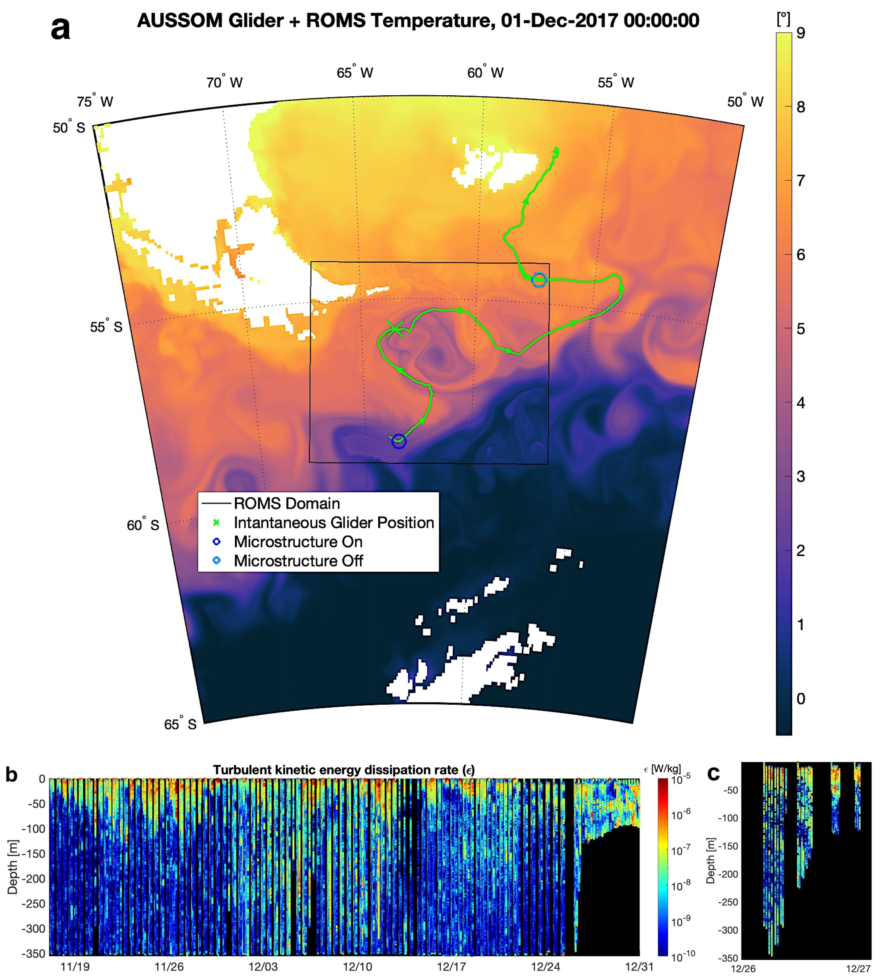
Figure 1. (a) Track of Slocum glider Starbuck along the Polar Front (PF) in Drake Passage and Scotia Sea during the AUSSOM project in late 2017 and early 2018. Temperature from ROMS is nested in temperature from 1/12° Operational Mercator. Note that the PF can merge with the Subantarctic Front in this region. (b) Showing observations of TKE dissipation rate collected by the glider. Elevated mixing is observed in the SBL, the subsurface core of the PF, and in proximity to sloping bathymetry (24-November onward). (c) A zoomed-in subset of (b) highlighting TKE dissipation near the bank.
2 Methods
For this basin-scale analysis, we use a criterion Equation 2 for overturning instability (Hoskins, 1974; Thomas et al., 2013) based on a balanced form of the Richardson number which assumes the dominance of geostrophic dynamics, :
Excluding barotropic inertial/centrifugal instabilities ,overturning instabilities arise when , where is the balanced Richardson number angle and is a critical angle (Thomas et al., 2013). Here ζa is the absolute vorticity and . The inverse tangent function can be approximated as a piecewise function such that discrete instability types are identified by the relative dominance of destabilizing characteristics, useful for the efficient identification of instability types (Table 1 reproduced from Thomas et al., 2013).
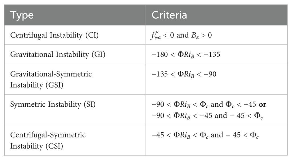
Table 1. Instability criteria.
Model output with 1-km, 3-hr resolution, and 50 sigma (σ) layers was produced using the Regional Ocean Modeling System (ROMS), a free-surface, hydrostatic, primitive equation model discretized with a terrain following vertical coordinate system (Shchepetkin and McWilliams, 2005). Runs were initialized every 7 days and run for 10 days, covering a period from 12-November-2017 through 29-December-2017. The model was initialized using 1/12° resolution Operational Mercator (GLOBAL_ANALYSIS_FORECAST_PHY_001_024) and radiation/nudging lateral boundary conditions and a 3-day relaxation timescale (Marchesiello et al., 2001). Flux forcing was computed every 3 hours with turbulent fluxes calculated from bulk formulae (Fairall et al., 1996; Large and Pond, 1981) using the atmospheric state obtained from JRA-55 (Tsujino et al., 2018), and no tidal forcing was imposed. The model utilized an orthogonal curvilinear grid that tracks latitude/longitude lines. Tracers and momentum use 3rd-order upstream-biased advection in the horizontal, and 4th-order centered differences advection in_the vertical. The model used GLS vertical mixing parameterization for turbulent mixing of momentum and tracers (Warner et al., 2005); with the Kantha and Clayson (1994) stability function, Craig and Banner (1994) wave breaking surface flux, and Charnok surface roughness from wind stress (Carniel et al., 2009). Horizontal diffusion of tracers and momentum were 2 m2/s and 3 m2/s respectively, with quadratic bottom friction coefficient of 0.003.
Upwind advection schemes contain implicit smoothing; dynamical processes below 5-km (rather than 2-km) are not well represented due to smoothing over the stencil, staggered grids, and time stepping. A limitation of using the 1-km ROMS model to study instability is its resolution constraints; submesoscale instabilities undoubtedly exist below the scales represented in the model. While symmetrically unstable flows may persist in the ocean due to forcing (e.g., FSI), another limitation of the model is that instabilities can persist longer in the model than the ocean due to lack of removal mechanisms (either a resolved forward energy cascade, or a parameterization for the unresolved forward energy cascade). We are confident that the westward velocity anomalies (relative to geostrophic flow) along the Bank which decrease stability are not simply pressure gradient errors (Mellor et al., 1998); which would manifest as a spurious addition of ∼0.01-0.1 m/s in the same direction as the geostrophic current (eastward, with the coast to the left). We also validate the results using a feature model to demonstrate the physical conditions leading to submesoscale instability (Appendix).
Vertical buoyancy (B) and velocity (U,V) profiles are linearly interpolated from σ-coordinates to a uniform vertical grid (Δz = 5 m) before calculation of spatial derivatives and the subsequent application of instability criteria (Table 1). The distribution of instability is examined from the perspective of meridional sections (conducive to study of the mainly-zonal PF jet), as well as the full 3-D domain. The latitude (ϕ) and velocity of the PF jet were obtained at the location of the maximum eastward component of velocity U(θ,ϕ,z) north of 56.5°S and within the longitudinal range for which the front and associated jet are dominantly zonal, 63.0°W< θ < 60.0°W. This region is selected for two reasons: The first is for ease of calculation on the model’s original grid, thus eliminating the step of projecting the jet velocity in the direction parallel to the coast while seeking the point of maximum along-coast velocity on a rotated grid. The second is to avoid obscuring signals in a basin-scale average. The jet can be different distances from the bank along different parts of the Drake Passage and Scotia Sea, which could blur regional trends in instability if examined in a basin-averaged sense. The purpose of the latitudinal constraint is to avoid misidentifying the SACCF jet core or (secondary filaments associated with the PF) as the PF jet core. A possible limitation of this method is that it neglects slight curvatures (relative angle) of Namuncurá - Burwood Bank and the PF jet, reducing the precision with which the reported latitude in 5c describes the jet’s proximity to the bank throughout the entire white box. We use longitude 60.5°W to illustrate meridional sections, but its features are common to meridional slices where the PF jet is principally zonal.
3 Results
As D’Asaro et al. (2011) and Thomas et al. (2013) hypothesized, submesoscale instabilities including CI, CSI, and SI are present in the upper ocean of the ACC (Figure 2a), both at the abrupt lateral buoyancy gradients of PF filaments and where submesoscale vortices are generated by interaction between the ACC and Tierra del Fuego and advected eastward. In the subsurface (Figure 2b), instabilities concentrate on the north side of the zonal jet (as predicted by geostrophic instability theory), but are tied to topography; these instabilities are found where the PF jet experiences topographic drag along Namuncurá - Burwood Bank. The position of the PF jet (Figure 3), namely, its proximity to the continental rise, controls the amount of subsurface CI, CSI, and SI. In general, a southern (northern) hemisphere process causing an increase (decrease) in relative vorticity increases (decreases) the potential vorticity toward symmetrically instability. Here, topographic drag on the north edge of the ACC (or alternatively, the southern flank of an abyssal feature) increases horizontal shear to create instability.
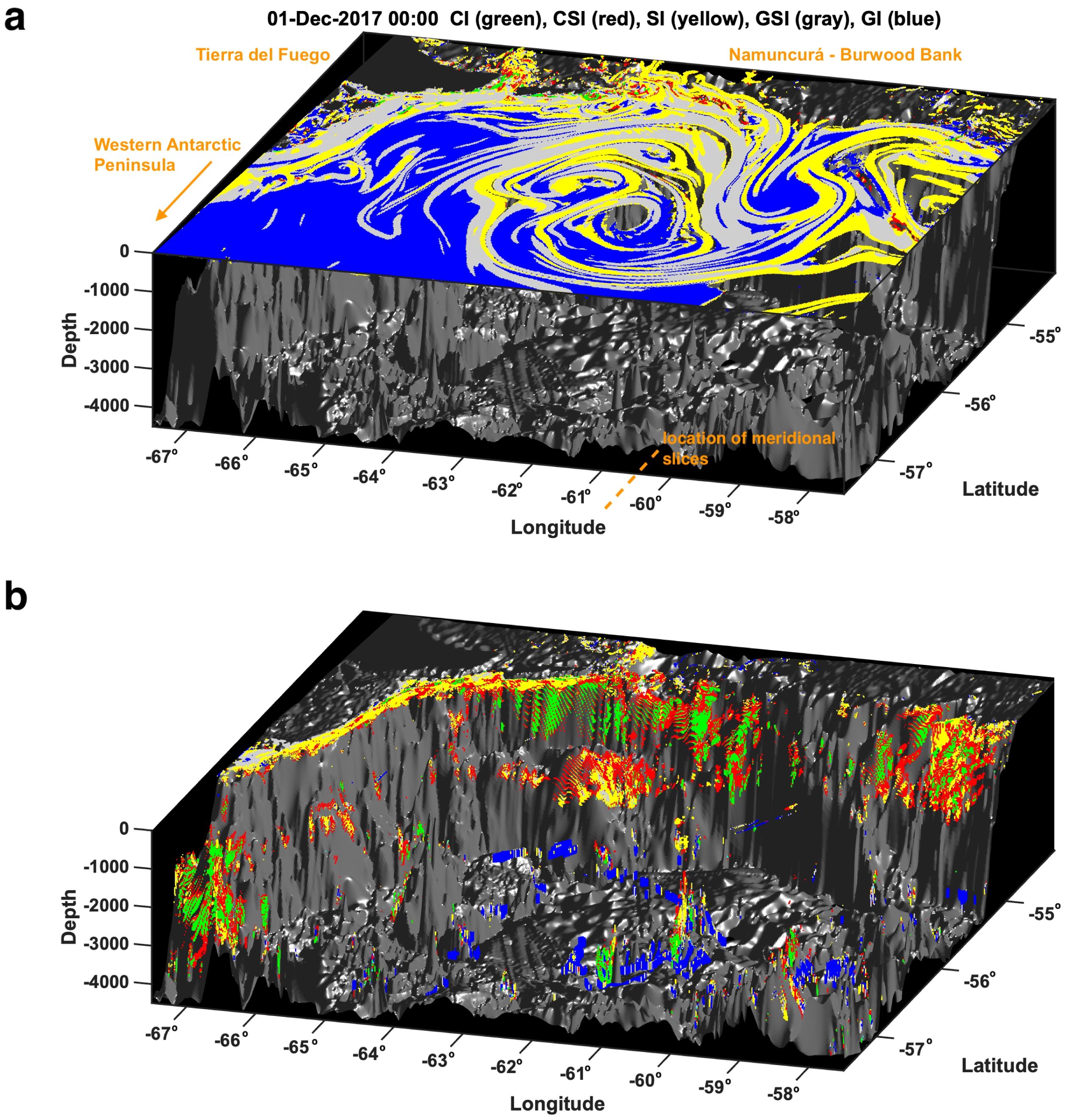
Figure 2. Showing unstable nodes in the (a) upper 100 m and (b) lower 100–4500 m for a timestep (01-Dec-2017) of the 3-D model domain; including gravitational (GI, blue), gravitational-symmetric (GSI, gray), centrifugal (CI, green), centrifugal-symmetric CSI, (red), and symmetric (SI, yellow) instability.
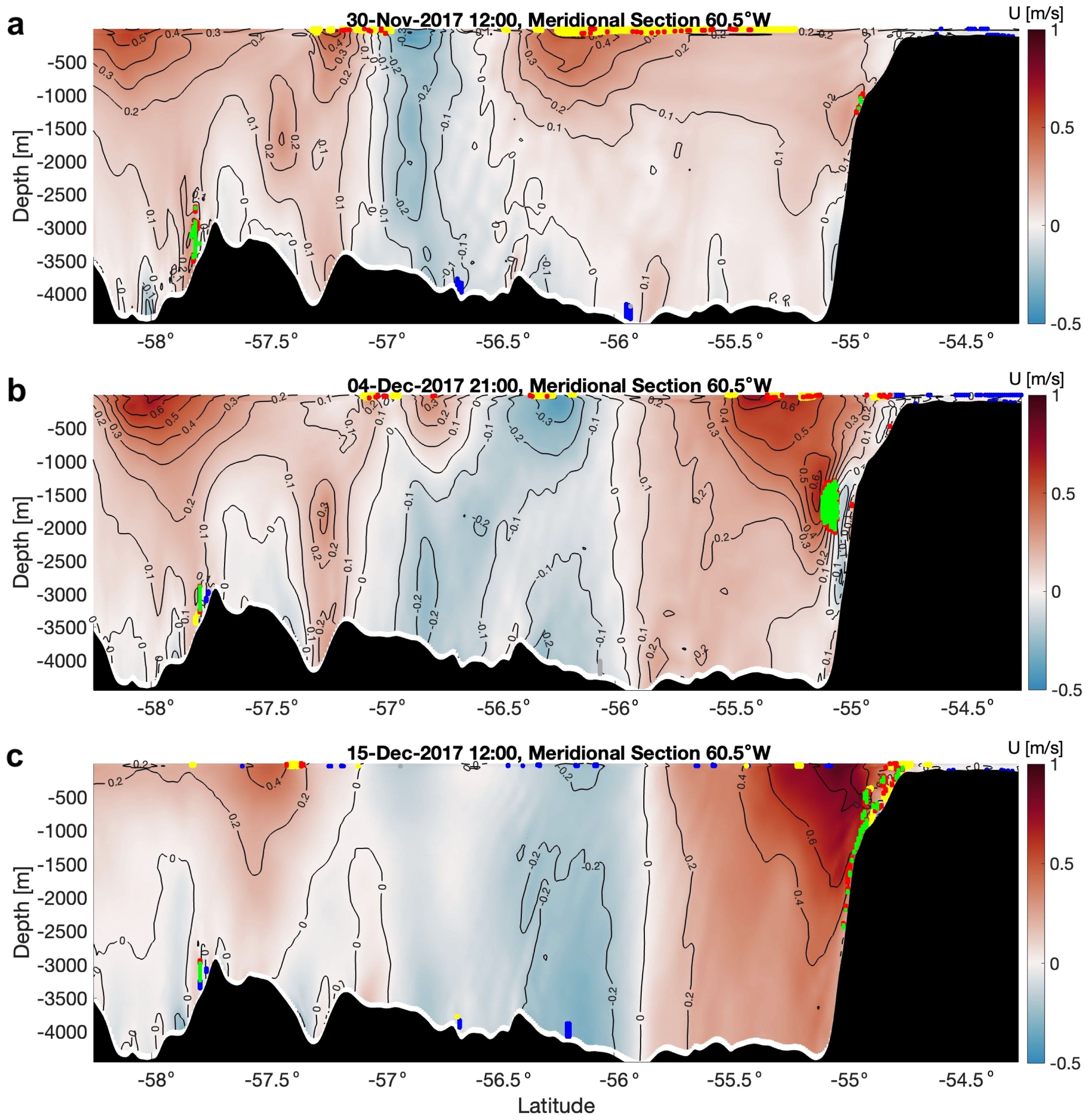
Figure 3. Phenomenology of centrifugal (CI, green), centrifugal-symmetric (CSI, red), symmetric (SI, yellow), gravitational-symmetric (GSI, gray), and gravitational (GI, blue) instabilities at 60.5°W (dotted line in Figure 2) for states of the PF jet with contours of eastward velocity (U). (a) Showing SI and CSI in the SBL, associated with Polar Front filaments. (b, c) Showing CSI, CI, and the added third characteristic in the subsurface, associated with flow-topography interaction along Tierra del Fuego and Namuncurá Burwood Bank.
The potential vorticity q Equation 1 in Figure 3 is decomposed into individual terms (Figure 4). We offer general context for these terms. q is the component of the absolute vorticity vector oriented with the buoyancy gradient (usually near-vertical in stably stratified fluids). Strong stratification Bz, large-magnitude planetary vorticity f, and relative vorticity in the same direction as f all reinforce the stability of the spinning column of fluid. In an adiabatic, frictionless flow q is materially conserved such that a fluid column moving toward weaker stratification or lower latitude must spin faster (Hoskins, 1997), which is accomplished by stretching of the column in the absence of viscosity. The spin can also be influenced directly by mechanical forcing. Tilting describes the action of vertical shear Uz,Vz to tip the horizontal vorticity. The decomposition in Figure 4 illustrates that the positive potential vorticity required for instability in the southern hemisphere is produced when vorticity of the fluid is spun in the anticyclonic direction (Figure 4b). Conversely, SI at open-ocean fronts is dependent on weak stratification (see pale layer in Figure 4a) for the production of net-positive potential vorticity and is thus confined to the weakly stratified SBL (∼0–100 m).
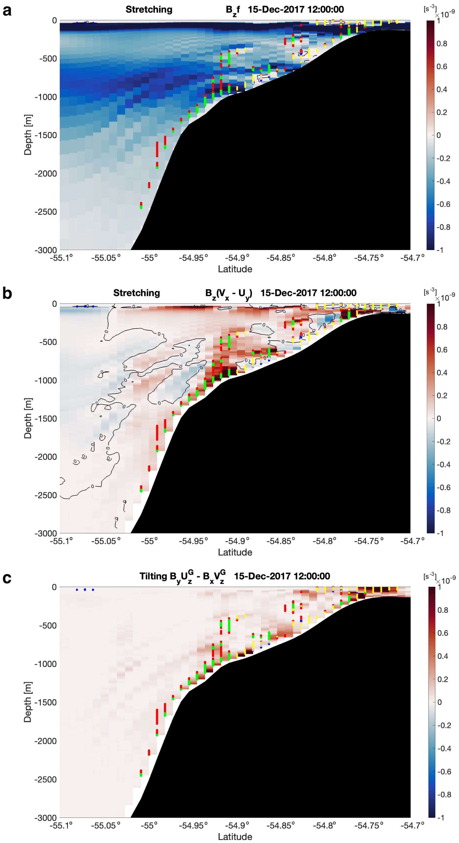
Figure 4. (a) Stretching related to planetary vorticity, (b) stretching related to relative vorticity, and (c) tilting terms [s−3] of Ertel potential vorticity (q, Equation 1) for the boundary region in 3c, where qf< 0 is unstable. Note axes have changed to zoom in on the depth and latitudinal range of interest. Positive values (red tones) are destabilizing, and negative values (blue tones) are stabilizing. The term illustrated in (b, a) is the primary driver of CSI (GSI). SI arises from combined effects of stretching (a, b) and tilting (c). Ribbon-like features are numerical artifacts typical of σ-coordinate models.
For the subset of the domain where the PF jet is principally zonal (see (Methods) and box in Figure 5a) we identify submesoscale instabilities (Figure 5b) in relation to latitude and speed of the PF (Figure 5c). Separating the domain into the shallow and subsurface ocean (Figures 5d, e) demonstrates two distinct instability regimes: an SBL dominated by classic shear-convective instability, and a subsurface ocean where CI and CSI contribute more greatly to the instability budget.
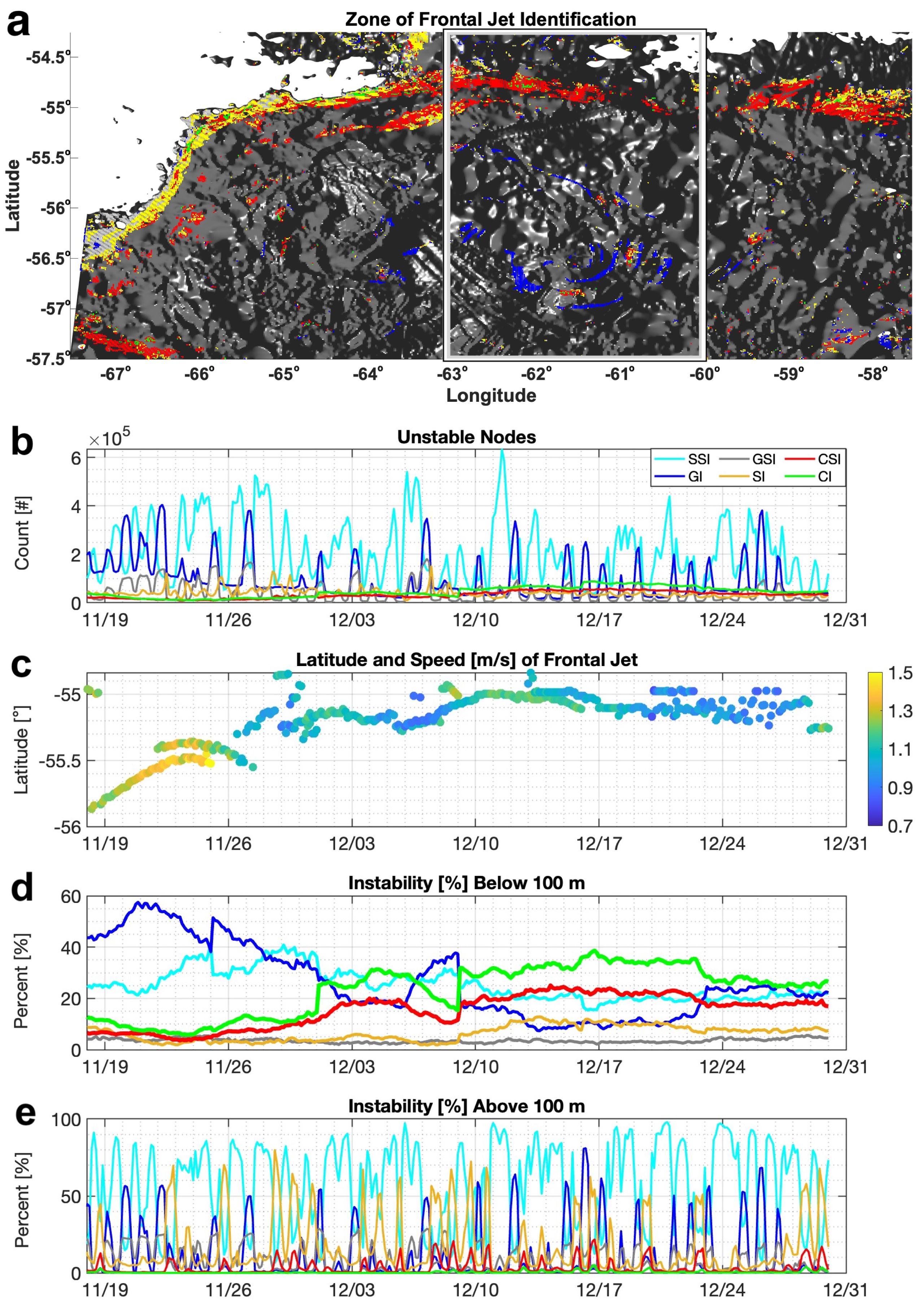
Figure 5. Instability compared to frontal jet variability. Showing (a) the region of instability identification (white box) superimposed over a top-down snapshot of the model (specifically the timestep in Figure 2b); (b) the number of uniformly interpolated grid nodes which are unstable to stratified shear instability (SSI), GI, GSI, SI, CSI, and CI; and (c) latitude and speed of the jet core. Namuncurá - Burwood Bank is located at ∼55°S. Additionally showing the relative prevalence of each instability type identified in both (d) the subsurface ocean and (e) the upper 100 m of the region. Note vertical discontinuities in (d) reflect the use of multiple model runs to cover the study period.
In the subsurface ocean (Figure 5d), the location of the PF jet and the associated mesoscale eddy present in the model (Figures 1a, 5a - box) control the relative role of each instability type to which the flow is predisposed. While the PF jet is shifted southward in late November, CI and CSI comprise about 10% of all overturning instabilities (as defined in the Figure 5 caption). While the PF shifts northward toward Namuncura´ - Burwood Bank (∼55°S) in the beginning of December, their relative role increases to about 30% and dominates the subsurface instability budget. Conversely, GI decreases as the front and mesoscale eddy shift northward. The GI arises in the modeled abyss (Figure 2b) when deep-reaching flow of the mesoscale eddy stirs dense bottom water equatorward to overlie lighter water; its setup depends on the proximity of the eddy to the bottom water at its poleward source. Its possible importance to abyssal mixing is beyond the scope of this paper but is worthy of future inquiry.
In the SBL (Figure 5e), the relative prevalence of each instability type is characterized by episodic surface evolution (Ferris et al., 2022a) as well as a diurnal oscillation produced by convective forcing in localized regions of the domain. The diurnal oscillation augments the total amount of both GI and GSI in the SBL and juxtaposes the steady nature of instability in the subsurface ocean (Figure 5d) — as with FSI due to winds (Dong et al., 2021b), topographic drag provides a mechanism for sustained overturning instability in the subsurface ocean. It is worth underscoring that analytical criteria in Table 1 are derived for a steady flow, such that they are meaningful only if instabilities grow on a timescale faster than the timescale at which the flow evolves. Diurnal variation of SI, GI, and GSI (Figure 5e) implies that some perceived instability in the SBL is transient and vanishes (by cessation of convective forcing and restratification) before undergoing forward energy cascade, such that some of the instability in Figure 5e is not physically meaningful. In other words, a convective instability arising in the final hours of night may not have time to grow before the SBL is stabilized by the arrival of day.
4 Discussion
Submesoscale instability is found at two major sites in the ACC: in the weakly stratified SBL, and in the subsurface ocean near lateral boundaries (or equivalently, sloping topography). The amount of subsurface submesoscale instability arising in ACC jets depends on their location with respect to topography, indicating that the importance of submesoscale instability to forward energy cascade in the ACC depends on temporal variation of the PF (unlike SBL instabilities which are not tied to geography of the PF). Furthermore, topographic shearing of the PF jet presents a mechanism for sustained CI, CSI, and SI (analogous to FSI in the upper ocean). Both atmospheric changes, such as the Southern Annular Mode and the El Nino˜ Southern Oscillation (ENSO), and internal dynamical variabilities alter the position of the ACC’s frontal jets on an intra-annual to inter-annual timescale (Gille et al., 2016). Altering the latitude of the ACC fronts with respect to Southern Ocean topography likely impacts the role of CI, CSI, and SI in mixing near surface and topographic boundaries (this study); as well as that of more ubiquitous internal wave processes [see Figures 4, 5 of St. Laurent et al. (2012); Waterhouse (2014)] which impact vertical heat, carbon, and nutrient flux throughout the Southern Ocean.
Our results inspire us to take an intellectual leap and speculate that submesoscale instabilities may play a role in the formation of Antarctic Intermediate Water (AAIW), a process that is not well understood. As part of the upper return cell of the Atlantic Meridional Overturning Circulation (Talley, 2013), air-sea exchange and interior mixing transform North Atlantic Deep Water (NADW) first into Subantarctic Mode Water (SAMW) and then into Antarctic Intermediate Water (AAIW). At the northern edge of the ACC in the vicinity of Namuncurá - Burwood Bank, a thick layer of SAWM overlies low-salinity AAIW, which overlies Upper Circumpolar Deep Water (UCDW). The Scotia Sea east of the Drake Passage is believed to be a critical site of SAMW and AAIW modification and subduction (Talley, 1996; Sallée et al., 2010), but little is known about their exact formation mechanisms. The CI, CSI, and SI discussed in this paper arise in the depth range appropriate for mixing AAIW with UCDW and SAMW (see Figure 1 of Struve et al., 2020). After observing a rich submesoscale frontal structure and upwelling/downwelling rates of O(100) m/day east of the Drake Passage, Adams et al. (2017) remarked that submesoscale processes might be critical for the transformation and subduction of mode and intermediate waters. We agree that further observations or turbulence-resolving models are needed to understand the significance of these instabilities at the northern continental margins of the ACC.
We ask whether some of the near-boundary elevated TKE (over rough topography and along continental margins) which was historically attributed to internal waves could be, in part, from submesoscale instabilities undergoing forward energy cascade. However, this is not the first finding of topographic shearing facilitating the forward energy cascade by producing submesoscale instabilities in a major current; (Gula et al., 2016) observed a similar mechanism. CI, CSI, and SI are created on the anticyclonic side of the ACC when topographic drag increases relative vorticity enough to destabilize the flow. If presence of northern boundary controls the development of instability, a natural conclusion is that the Drake Passage and Scotia Sea region are unique to the rest of the ACC (perhaps with the exceptions of the Agulhas Bank and Campbell Plateau); however, other features such as the Antarctic Slope Current and Kerguelen Plateau (as well as submerged seamounts in currents across the global ocean, such as the New England Seamount Chain in the Gulf Stream) provide topographic drag and are thus candidates for topographic forcing of submesoscale instability. Despite being tied to specific topographic features, evidence for the spatial inhomogeneity of Southern Ocean mixing (Whalen et al., 2015; Tamsitt et al., 2017) shows that the spatial extent of a particular mixing mechanism does not equate to its overall impact. Topographically-sheared instabilities in the ACC may disproportionately affect mixing.
It is worth noting, however, that a significant amount of mixing in the Southern Ocean, especially in the subsurface open ocean, is not due to topographically forced CI, CSI, and SI — or any kind of submesoscale instability (Ferris et al., 2022a). We briefly revisit the glider data (Figure 1b), which shows turbulence in the SBL and subsurface ocean near the Bank (regimes where submesoscale instability occurs); as well as an unidentified patch of turbulence in the subsurface open ocean. The latter is likely not from submesoscale instability based on our analysis. While the amount of TKE produced by SI in the SBL is indeed consistent with the levels of turbulence observed by the glider (Figure 6), this subsurface feature cannot be attributable to CI, CSI, or SI due to the limited vertical influence (depth range 0< z< 100 m) of these instabilities away from topographic boundaries. We speculate it is related to internal wave interactions at the margins of Polar Front jets.
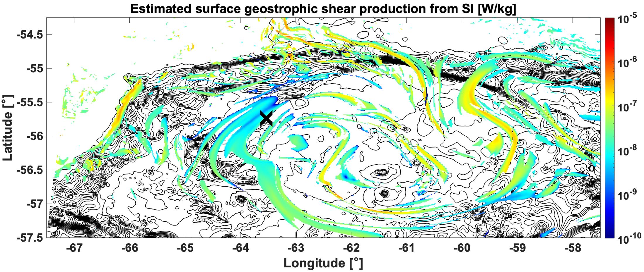
Figure 6. Estimated geostrophic shear production for the timestep in Figure 2 (01-Dec-2017), estimated after (Thomas et al., 2013; Bachman et al., 2017; Dong et al., 2021b). Bathymetric contours are underlaid at 300-m intervals and the instantaneous location of the glider (Figure 1b is marked with a cross.
We have provided insight into the relative role and spatial arrangement of symmetric instabilities in the Southern Ocean, finding that submesoscale overturning instabilities may be as important along the topographic boundaries of the ACC as they are at fronts in the SBL of the open ocean. This finding is relevant to other energetic currents rich in frontal structure; instability analysis of the Kuroshio and Gulf Stream are relatively uncommon similar to the ACC, and there has been little submesoscale instability work in the subarctic (which is similarly rich in energetic filaments, complex topography, and sharp density fronts). The inclusion of topographically sheared submesoscale instabilities may be important for modeling ocean structure in several coastal and littoral regions of the world. Meanwhile, the overall velocity structure in many of these regions is altered by tides with short periods or diurnal convection, complicating the applicability of existing balanced frameworks. This will be a topic of future investigation.
This study and others (Dewar et al., 2015; Gula et al., 2016; Wenegrat and Thomas, 2020; Yankovsky et al., 2021) are strong support that traditionally surface-associated submesoscale frontal instabilities can arise below the SBL when forced by topography; and if parameterized in ocean models, should be treated as more than just an SBL effect. Our results suggest SI below the SBL is ubiquitous in topographically sheared frontal regions, indicating that subsurface parameterization (e.g., Yankovsky et al., 2021) is useful in regions with complex topography. This said, we emphasize that the presence of unstable flow does not guarantee that SI or its hybrid types will grow on a meaningful timescale or produce a TKE contribution (Ferris and Gong, 2024). An open task is to estimate the mixing efficiency associated with topographically forced submesoscale instability (Ijichi et al., 2020), and its relative role (if any) in driving upper ocean structure. The community’s need to develop realistic parameterizations for unresolved submesoscale instability is strong motivation to make further observations in regions suspected of topographically-sheared SI, CSI, and CI; and to better understand the growth rates, depths, and re-stratification timescales associated with these instabilities in the real ocean. At the same time, equal focus should be placed on classic shear turbulence and internal wave phenomena in the Southern Ocean, which are likely as important (if not more important) than submesoscale instability away from boundaries.
Data availability statement
ROMS model output is archived with William & Mary Scholar Works (https://doi.org/10.25773/8wqm-7r04). Operational Mercator used for the ROMS (https://github.com/myroms) model is made freely available by the EU Copernicus Marine Service (https://marine.copernicus.eu/).
Author contributions
LF: Methodology, Writing – original draft, Conceptualization. DG: Supervision, Writing – review & editing. JK: Writing – review & editing, Methodology.
Funding
The author(s) declare financial support was received for the research and/or publication of this article. Ferris’s effort was funded by the Virginia Institute of Marine Science (VIMS) Office of Academic Studies as well as the Applied Physics Laboratory - University of Washington Science & Engineering Enrichment & Development (SEED) Fellowship.
Acknowledgments
AUSSOM microstructure data is used courtesy of Louis St. Laurent and was supported by the OCE Division of the National Science Foundation, award 1558639 (PIs St. Laurent and Sophia Merrifield). ROMS output is used courtesy of Harper Simmons and John Pender, for which computational resources were provided by Research Computing Systems at University of Alaska Fairbanks. We thank the VIMS Ocean-Atmosphere & Climate Change Research Fund (Emeritus John Boon) for his gift of a computer. We thank Justin Shapiro and Thilo Klenz for sharing technical expertise.
Conflict of interest
The authors declare that the research was conducted in the absence of any commercial or financial relationships that could be construed as a potential conflict of interest.
The author(s) declared that they were an editorial board member of Frontiers, at the time of submission. This had no impact on the peer review process and the final decision.
Generative AI statement
The author(s) declare that no Generative AI was used in the creation of this manuscript.
Any alternative text (alt text) provided alongside figures in this article has been generated by Frontiers with the support of artificial intelligence and reasonable efforts have been made to ensure accuracy, including review by the authors wherever possible. If you identify any issues, please contact us.
Publisher’s note
All claims expressed in this article are solely those of the authors and do not necessarily represent those of their affiliated organizations, or those of the publisher, the editors and the reviewers. Any product that may be evaluated in this article, or claim that may be made by its manufacturer, is not guaranteed or endorsed by the publisher.
Supplementary material
The Supplementary Material for this article can be found online at: https://www.frontiersin.org/articles/10.3389/fmars.2025.1612637/full#supplementary-material
Supplementary Figure 1 | Cross-sections of an idealized jet for the near-boundary case. Nodes satisfying criteria (Table 1) for centrifugal (green) and centrifugal-symmetric instability (red) are highlighted (F). There are no instances of pure symmetric instability.
Supplementary Figure 2 | Cross-sections of an idealized jet for the near-boundary case. As in Supplementary Figure A1, nodes satisfying criteria (Table 1) for centrifugal (green) and centrifugal-symmetric instability (red) are highlighted (f). There are no instances of pure symmetric instability.
References
Adams K. A., Hosegood P., Taylor J. R., Sallée J. B., Bachman S., Torres R., et al. (2017). Frontal circulation and submesoscale variability during the formation of a southern ocean mesoscale eddy. J. Phys. Oceanography 47, 1737–1753. doi: 10.1175/JPO-D-16-0266.1
Bachman S., Fox-Kemper B., Taylor J., and Thomas L. (2017). Parameterization of frontal symmetric instabilities. I: Theory for resolved fronts. Ocean Model. 109, 72–95. doi: 10.1016/j.ocemod.2016.12.003
Carniel S., Warner J., Chiggiato J., and Sclavo M. (2009). Investigating the impact of surface wave breaking on modeling the trajectories of drifters in the northern adriatic sea during a wind-storm event. Ocean Model. 30, 225–239. doi: 10.1016/j.ocemod.2009.07.001
Chor T., Wenegrat J., and Taylor J. (2022). Insights into the mixing efficiency of submesoscale centrifugal–symmetric instabilities. J. Phys. Oceanography 52, 2273–2287. doi: 10.1175/JPO-D-21-0259.1
Craig P. and Banner M. (1994). Modeling wave-enhanced turbulence in the ocean surface layer. J. Phys. Oceanography 24, 2546–2559. doi: 10.1175/1520-0485(1994)024<2546:MWETIT>2.0.CO;2
D’Asaro E., Lee C., Rainville L., Thomas L., and Harcourt R. (2011). Enhanced turbulence and energy dissipation at ocean fronts. Science 322 (6027), 318–322. doi: 10.1126/science.1201515
Dewar W., McWilliams J., and Molemaker M. (2015). Centrifugal instability and mixing in the california undercurrent. J. Phys. Oceanography 45, 1224–1241. doi: 10.1175/JPO-D-13-0269.1
Dong J., Fox-Kemper B., Zhang H., and Dong C. (2021a). The scale and activity of symmetric instability estimated from a global submesoscale-permitting ocean model. J. Phys. Oceanogr. 51, 1655–1670. doi: 10.1175/JPO-D-20-0159.1
Dong J., Fox-Kemper B., Zhu J., and Dong C. (2021b). Application of symmetric instability parameterization in the coastal and regional ocean community model (croco). J. Adv. Modeling Earth Syst. 13, e2020MS002302. doi: 10.1029/2020MS002302
Fairall C. W., Bradley E. F., Rogers D. P., Edson J. B., and Young G. S. (1996). Bulk parameterization of air-sea fluxes for tropical ocean-global atmosphere coupled-ocean atmosphere response experiment. J. Geophysical Research: Oceans 101, 3747–3764. doi: 10.1029/95JC03205
Fer I., Peterson A., and Ullgren J. (2014). Microstructure measurements from an underwater glider in the turbulent faroe bank channel overflow. J. Atmospheric Oceanic Technol. 31, 1128–1150. doi: 10.1175/JTECH-D-13-00221.1
Ferris L. (2022). Across-scale energy transfer in the Southern Ocean. Ph.D. thesis (Virginia Institute of Marine Science - William and Mary. Ph.D. Dissertation), 190.
Ferris L. and Gong D. (2024). Damping effects of viscous dissipation on growth of symmetric instability. arXiv [physics.ao-ph]. Available online at: http://arxiv.org/abs/2406.16818.
Ferris L., Gong D., Clayson C., Merrifield S., Shroyer E., Smith M., et al. (2022a). Shear turbulence in the high-wind southern ocean using direct measurements. J. Phys. Oceanography 52, 2325–2341. doi: 10.1175/JPO-D-21-0015.1
Ferris L., Gong D., Merrifield S., and St. Laurent L. (2022b). Contamination of finescale strain estimates of turbulent kinetic energy dissipation by frontal physics. J. Atmospheric Oceanic Technol. 39, 619–640. doi: 10.1175/JTECH-D-21-0088.1
Firing Y. (2020). “RRS discovery cruise DY113, 3 february–13 march 2020,” in Repeat hydrographic measurements on GO-SHIP lines SR1b and A23.
Gangopadhyay A. and Robinson A. (2002). Feature-oriented regional modeling of oceanic fronts. Dynamics Atmospheres Oceans 36, 201–232. doi: 10.1016/S0377-0265(02)00032-5
Gille S., McKee D., and Martinson D. (2016). Temporal changes in the antarctic circumpolar current: Implications for the antarctic continental shelves. Oceanography 29, 96–105. doi: 10.5670/oceanog.2016.102
Goldsworth F. W., Johnson H. L., Marshall D. P., and Le Bras I. A. (2024). Destratifying and restratifying instabilities during down-front wind events: A case study in the irminger sea. J. Geophysical Research: Oceans 129, e2023JC020365. doi: 10.1029/2023JC020365
Gula J., Molemaker M., and McWilliams J. (2016). Topographic generation of submesoscale centrifugal instability and energy dissipation. Nat. Commun. 7, 1–7. doi: 10.1038/ncomms12811
Hoskins B. (1974). The role of potential vorticity in symmetric stability and instability. Q. J. R. Meteorological Soc. 100, 480–482. doi: 10.1002/qj.49710042520
Hoskins B. (1997). A potential vorticity view of synoptic development. Meteorological Appl. 4, 325–334. doi: 10.1017/S1350482797000716
Ijichi T., St. Laurent L., Polzin K., and Toole J. (2020). How variable is mixing efficiency in the abyss? Geophysical Res. Lett. 47, e2019GL086813. doi: 10.1029/2019GL086813
Jiao Y. and Dewar W. K. (2015). The energetics of centrifugal instability. J. Phys. Oceanography 45, 1554–1573. doi: 10.1175/JPO-D-14-0064.1
Kantha L. and Clayson C. (1994). An improved mixed layer model for geophysical applications. J. Geophysical Research: Oceans 99, 25235–25266. doi: 10.1029/94JC02257
Large W. G., McWilliams J. C., and Doney S. C. (1994). Oceanic vertical mixing: A review and a model with a nonlocal boundary layer parameterization. Rev. Geophysics 32, 363–403. doi: 10.1029/94RG01872
Large W. G. and Pond S. (1981). Open ocean momentum flux measurements in moderate to strong winds. J. Phys. Oceanography 11, 324–336. doi: 10.1175/1520-0485(1981)011<0324:OOMFMI>2.0.CO;2
Lenton A. and Matear R. J. (2007). Role of the southern annular mode (sam) in southern ocean co2 uptake. Global Biogeochemical Cycles 21. doi: 10.1029/2006GB002714
Liau J. and Chao B. (2017). Variation of antarctic circumpolar current and its intensification in relation to the southern annular mode detected in the time-variable gravity signals by grace satellite. Earth Planets Space 69, 1–9. doi: 10.1186/s40623-017-0678-3
Marchesiello P., McWilliams J., and Shchepetkin A. (2001). Open boundary conditions for long-term integration of regional oceanic models. Ocean Model. 3, 1–20. doi: 10.1016/S1463-5003(00)00013-5
Mashayek A., Ferrari R., Merrifield S., Ledwell J., St. Laurent L., and Garabato A. (2017). Topographic enhancement of vertical turbulent mixing in the southern ocean. Nat. Commun. 8, 1–12. doi: 10.1038/ncomms14197
Mellor G., Oey L., and Ezer T. (1998). Sigma coordinate pressure gradient errors and the seamount problem. J. Atmospheric Oceanic Technol. 15, 1122–1131. doi: 10.1175/1520-0426(1998)015<1122:SCPGEA>2.0.CO;2
Mellor-Yamada T. (1982). Development of a turbulence closure model for geophysical fluid problems. Rev. Geophysics 20, 851–875. doi: 10.1029/RG020i004p00851
Meredith M. and Hogg A. (2006). Circumpolar response of southern ocean eddy activity to a change in the southern annular mode. Geophysical Res. Lett. 33. doi: 10.1029/2006GL026499
Naveira Garabato A., Frajka-Williams E., Spingys C., Legg S., Polzin K., Forryan A., et al. (2019). Rapid mixing and exchange of deep-ocean waters in an abyssal boundary current. Proc. Natl. Acad. Sci. 116, 13233–13238. doi: 10.1073/pnas.1904087116
Rosso I., Hogg A. M., Kiss A. E., and Gayen B. (2015). Topographic influence on submesoscale dynamics in the southern ocean. Geophysical Res. Lett. 42, 1139–1147. doi: 10.1002/2014GL062720
Sallée J. B., Speer K., Rintoul S., and Wijffels S. (2010). Southern ocean thermocline ventilation. J. Phys. Oceanography 40, 509–529. doi: 10.1175/2009JPO4291.1
Shchepetkin A. F. and McWilliams J. C. (2005). The regional oceanic modeling system (roms): a splitexplicit, free-surface, topography-following-coordinate oceanic model. Ocean Model. 9, 347–404. doi: 10.1016/j.ocemod.2004.08.002
Simmons H., Powell B., Merrifield S., Zedler S., and Colin P. (2019). Dynamical downscaling. Oceanography 32, 84–91. doi: 10.5670/oceanog.2019.414
St. Laurent L., Ijichi T., Merrifield S., Shapiro J., and Simmons H. (2019). Turbulence and vorticity in the wake of Palau. Oceanography 32, 102–109. doi: 10.5670/oceanog.2019.416
St. Laurent L. and Merrifield S. (2017). Measurements of near-surface turbulence and mixing from autonomous ocean gliders. Oceanography 30, 116–125. doi: 10.5670/oceanog.2017.231
St. Laurent L., Naveira Garabato A. C., Ledwell J. R., Thurnherr A. M., Toole J. M., and Watson A. J. (2012). Turbulence and diapycnal mixing in drake passage. J. Phys. Oceanography 42, 2143–2152. doi: 10.1175/JPO-D-12-027.1
Struve T., Wilson D. J., van de Flierdt T., Pratt N., and Crocket K. C. (2020). Middle holocene expansion of pacific deep water into the southern ocean. Proc. Natl. Acad. Sci. 117, 889–894. doi: 10.1073/pnas.1908138117
Talley L. D. (1996). “Antarctic intermediate water in the south atlantic,” in The south atlantic (Springer, Berlin, Heidelberg), 219–238.
Talley L. D. (2013). Closure of the global overturning circulation through the Indian, pacific, and southern oceans: Schematics and transports. Oceanography 26, 80–97. doi: 10.5670/oceanog.2013.07
Tamsitt V., Drake H. F., Morrison A. K., Talley L. D., Dufour C. O., Gray A. R., et al. (2017). Spiraling pathways of global deep waters to the surface of the southern ocean. Nat. Commun. 8, 172. doi: 10.1038/s41467-017-00197-0
Thomas L., Tandon A., and Mahadevan A. (2008). “Submesoscale processes and dynamics,” in Ocean modeling in an eddying regime, vol. 177. (American Geophysical Union), 17–38.
Thomas L., Taylor J., D’Asaro E., Lee C., Klymak J., and Shcherbina A. (2016). Symmetric instability, inertial oscillations, and turbulence at the gulf stream front. J. Phys. Oceanography 46, 197–217. doi: 10.1175/JPO-D-15-0008.1
Thomas L., Taylor J., Ferrari R., and Joyce T. (2013). Symmetric instability in the gulf stream. Deep Sea Res. Part II: Topical Stud. Oceanography 91, 96–110. doi: 10.1016/j.dsr2.2013.02.025
Todd R., Owens W., and Rudnick D. (2016). Potential vorticity structure in the north atlantic western boundary current from underwater glider observations. J. Phys. Oceanography 46, 327–348. doi: 10.1175/JPO-D-15-0112.1
Tsujino H., Urakawa S., Nakano H., Small R., Kim W., Yeager S., et al. (2018). Jra-55 based surface dataset for driving ocean–sea-ice models (jra55-do). Ocean Model. 130, 79–139. doi: 10.1016/j.ocemod.2018.07.002
Warner J., Sherwood C., Arango H., and Signell R. (2005). Performance of four turbulence closure models implemented using a generic length scale method. Ocean Model. 8, 81–113. doi: 10.1016/j.ocemod.2003.12.003
Waterhouse, E. A., A. F (2014). Global patterns of diapycnal mixing from measurements of the turbulent dissipation rate. J. Phys. Oceanography 44, 1854–1872. doi: 10.1175/JPO-D-13-0104.1
Wenegrat J. O., Callies J., and Thomas L. N. (2018). Submesoscale baroclinic instability in the bottom boundary layer. J. Phys. Oceanography 48, 2571–2592. doi: 10.1175/JPO-D-17-0264.1
Wenegrat J. and Thomas L. (2020). Centrifugal and symmetric instability during ekman adjustment of the bottom boundary layer. J. Phys. Oceanography 50, 1793–1812. doi: 10.1175/JPO-D-20-0027.1
Whalen C. B., MacKinnon J. A., Talley L. D., and Waterhouse A. F. (2015). Estimating the mean diapycnal mixing using a finescale strain parameterization. J. Phys. Oceanography 45, 1174–1188. doi: 10.1175/JPO-D-14-0167.1
Wienkers A., Thomas L., and Taylor J. (2021). The influence of front strength on the development and equilibration of symmetric instability. part 1. growth and saturation. J. Fluid Mechanics 926. doi: 10.1017/jfm.2021.680
Yankovsky E., Legg S., and Hallberg R. (2021). Parameterization of submesoscale symmetric instability in dense flows along topography. J. Adv. Modeling Earth Syst. 13(6), e2020MS002264. doi: 10.1029/2020MS002264
Appendix
We validate the results of the 1-km ROMS hindcast using velocity-based feature model after (Gangopadhyay and Robinson, 2002). A 2D idealized model (Table A1), based on a PF-associated jet observed during AUSSOM, was created from the geometry observed via AVISO, wind conditions from CCMP V2.0, and approximate density from the glider to investigate the development of instability. The model is a cross-section of a geostrophic zonal jet with no time evolution. The background density structure (ρθ) based on a Drake Passage width of LDP = 850 km and potential density anomaly () which produce the geostrophic jet are given by (Equation A1a, A1b):
where and and width of the anomaly (Δyρ) is 7 km, resulting in stratification N2 = 3 × 10⁻⁶s−2. The latitude of the density anomaly is chosen to be 100 km (Case Ocean, representing an open ocean jet) or 170 km (Case Boundary, representing near-boundary jet). The jet velocity (U0 ≤ 1.37 m/s) is calculated using thermal wind balance , where and subscripts indicate differentiated quantities. A horizontal velocity anomaly δU ≥ −0.35 m/s (Equation A2b) and logarithmic decay function are used to represent the effects of topographic shearing (Equation A2c). The horizontal velocity anomaly is equivalent to representing the effects of a topographic form drag using the expression for wall vorticity, .
The physical presence of topographic shearing along Namuncurá - Burwood Bank is supported by two datasets: (a) a weak westward flow 0.1-0.2 m/s was observed in the 2020 reoccupation of GO-SHIP sections SR1B and A23 across the Drake Passage and Scotia Sea (Firing, 2020), and (b) a westward velocity anomaly (intermittently amounting to a westward flow, e.g. Figure 3b) of similar magnitude arises in our ROMS model.
Here (Equation A2b, A2c) and ΔyU = 3 km. Omitting the topographic boundary layer, the transport is similar for both idealized scenarios; 30.73 Sv for Case Ocean and 30.87 Sv for Case Boundary.
Cross-sections of the jet in both cases are provided (Supplementary Figures A1, A2) with instabilities (Table 1) highlighted over Ertel potential vorticity. In Case Ocean (Supplementary Figure A1), stratification effects create CSI which doubles the total amount of overturning instability that would otherwise be limited to CI. In Case Boundary (Supplementary Figure A2), close proximity of the jet to the northern boundary increases the instances of CI, which is augmented by a doubling in CSI. The CSI extends throughout the water column, illustrating it is not a process specific to the surface ocean as commonly intuited. This feature model validates the conclusion derived from the ROMS model, that an otherwise identical jet can produce different amounts of subsurface submesoscale instability depending on its location relative to topography.
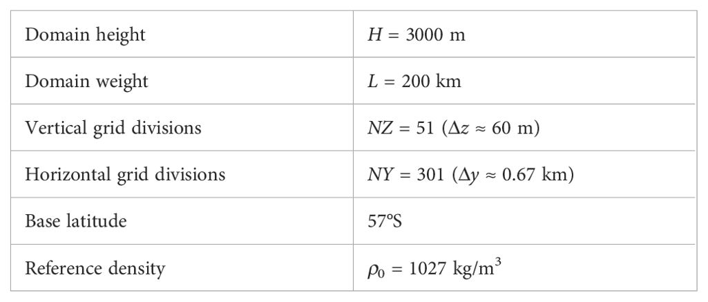
Table A1. Parameters for 2D model.
Keywords: submesoscale, instability, flow-topography interaction, mixing, Antarctic Circumpolar Current
Citation: Ferris L, Gong D and Klinck J (2025) Topographic forcing of submesoscale instability in the Antarctic Circumpolar Current. Front. Mar. Sci. 12:1612637. doi: 10.3389/fmars.2025.1612637
Received: 16 April 2025; Accepted: 22 July 2025;
Published: 25 September 2025.
Edited by:
Anna Olivé Abelló, Spanish National Research Council (CSIC), SpainReviewed by:
Tien Anh Tran, Seoul National University, Republic of KoreaChristopher Auckland, University of East Anglia, United Kingdom
Copyright © 2025 Ferris, Gong and Klinck. This is an open-access article distributed under the terms of the Creative Commons Attribution License (CC BY). The use, distribution or reproduction in other forums is permitted, provided the original author(s) and the copyright owner(s) are credited and that the original publication in this journal is cited, in accordance with accepted academic practice. No use, distribution or reproduction is permitted which does not comply with these terms.
*Correspondence: Laur Ferris, bG5mZXJyaXNAdmltcy5lZHU=