Modelling the spatial bound of an eDNA signal in the marine environment – the effect of local conditions

Environmental DNA (eDNA) is a powerful technique for biological assessments and monitoring in aquatic environments. The accurate interpretation of the source of eDNA detected requires understanding of its spatial and temporal bound. Studies which estimate eDNA dispersal in the aquatic environment, in particular the marine environment, are scarce and seldom represent the effect of hydrodynamics and eDNA decay. This study modelled eDNA dispersal in a coastal environment under diverse environmental conditions to assess how these conditions influence dispersal patterns. A modelling experiment shows that under thermally stratified conditions sampling eDNA across this gradient reduces detectability. Statistical analysis shows that both median and extreme eDNA dispersal distances simulated by the model were primarily controlled by local tidal conditions (tidal excursion), followed by month (influencing the water temperature and thus eDNA decay rate). The median distance varies between 2.27 and 14.14 km which falls within the range of previously published model results, and is up to 10x greater than observed values. However this gap has been narrowing, and the present statistical model helps set limits on the distance to source as a function of regional oceanography and water temperature. The present method can also be used post-survey to help interpret the location and number of sources. This study constitutes an advance in modelling eDNA dispersal in coastal areas and crucially provides much needed evidence to underpin robust interpretation of eDNA monitoring data and to inform the design of eDNA monitoring programmes that account for variable environmental conditions.

1 Introduction

Environmental DNA (eDNA) refers to DNA from organisms that is present in the environment. eDNA enters the environment through shedding, excretion, sloughing or via injury (Thomsen and Willerslev, 2015). DNA can be extracted, amplified and sequenced from environmental samples (e.g. water, soil, sediment), allowing the identification of the source species.

Monitoring the state and health of the environment is crucial for assessing the effectiveness of management actions and ensuring compliance with key legislation. Driven by multiple policies and legislative frameworks, environmental monitoring is often broad in scope and includes the assessment of biodiversity, community composition, and specific species presence and abundance, both vulnerable and invasive species. In the marine environment, such monitoring was traditionally dependent on expensive, time consuming, logistically and scientifically challenging techniques. However, over the last decade or so, interest in the application of eDNA for marine biodiversity monitoring has exploded. While uptake in academic settings reflects growing interest, adoption by managers and policymakers has been somewhat slower (Fonseca et al., 2023; Darling, 2019).

One of the limitations commonly cited with respect to eDNA is a lack of certainty around the relationship between an eDNA signal and its source organism (Ellis et al., 2022; Hansen et al., 2018), with consequences for the interpretation of monitoring results using eDNA methodologies. Understanding and predicting the transport of eDNA and spatial and temporal bounds of an eDNA signal is important for its uptake as a tool for marine monitoring. For example, management responses may vary depending on whether the identified organism is located within or outside a Marine Protected Area. Additionally, the responsibility for management or response to an incursion may depend on a spatial extent of the signal relative to jurisdictional boundaries.

The spatial relationship between an eDNA signal and its source is driven by three key factors: shedding; transport; and decay, often referred to collectively as the ecology of eDNA (Barnes and Turner, 2016). While transport through biological, i.e. predator-prey, interactions (Barnes and Turner, 2016; Sassoubre et al., 2016) or anthropogenic vectors, such as ballast water (Ardura et al., 2015; Egan et al., 2015) may occur, transport of eDNA vertically and horizontally in the marine environment is predominantly controlled by abiotic factors such as currents, tides, and hydrodynamic mixing (Foote et al., 2012; Port et al., 2016; Thomsen and Willerslev, 2015). eDNA decay plays a major role in determining the distance between an eDNA detection and its source organism. While it is challenging to disentangle study specific factors from global factors affecting eDNA decay, recent evidence suggests that eDNA decay is dependent on both temperature and salinity, with faster decay correlated with higher temperatures and higher salinity (i.e. in the marine environment compared to the freshwater environment) (Lamb et al., 2022).

Many studies document good concordance between eDNA data and traditional survey data, even at fine spatial resolution. For example, eDNA distinguished between coastal vertebrate communities in Monterey Bay, CA, United States, present along a gradation of diverse marine habitats including kelp forests,< 60 m apart (Port et al., 2016), and a statistically significant relationship between eDNA signals and visual detection was found for the Chilean devil ray, Mobula tarapacana, in the Azores (Gargan et al., 2017). Further, differences in eDNA signals between surface samples and seafloor samples (Andruszkiewicz et al., 2017; Lacoursière-Roussel et al., 2018; Uthicke et al., 2018; Yamamoto et al., 2017), and distinct vertical stratifications have been documented (Jeunen et al., 2019). However, there is substantial variation in eDNA transport estimates in the aquatic environment, with distances from meters to hundreds of kilometres reported (Deiner and Altermatt, 2014; Jane et al., 2014; Pont et al., 2018; Sansom and Sassoubre, 2017; Shogren et al., 2017).

Measures of eDNA transport in rivers have been used to help choosing sampling locations (Jo and Yamanaka, 2022). This serves both to avoid False-positives created by organisms upstream (e.g. from a river feeding into a lake) and False-negatives by making sure that sampling is close enough to the sources to be detected. A minimum distance from source has also been studied for rivers (Wood Z. T. et al., 2021) which is influenced by the time needed for the eDNA sample to break down and mix in the water, allowing some of it to be captured during downstream sampling.

Modelling provides an opportunity to examine the spatial relationship between an eDNA signal and its source, in particular modelling that integrates molecular ecology with hydrodynamics (Dawson et al., 2005). Particle tracking modelling involves spatial simulation of physical advection and diffusion of parcels of water informed by hydrodynamic fields, combined with biological trait input (e.g. Wood L. E. et al., 2021). By parameterising a parcel to reflect a volume of water with a certain eDNA concentration, in particular accounting for traits such as buoyancy, settlement, size and decay rate, particle tracking modelling can be used to quantitatively predict the dispersal of eDNA from a source location. In addition to providing useful outputs to address the spatial relationship between an eDNA signal and its source, such models can be used to elucidate factors crucial to eDNA dispersal (via parameter sensitivity), thereby informing prioritisation of further research to address remaining knowledge gaps. Though recently applied to examine transport of Californian anchovy Engraulis mordax in Monterey Bay (Andruszkiewicz et al., 2019), cold-water coral Lophelia pertusa in Norwegian fjords (Kutti et al., 2020) and two invasive species, kelp Undaria pinnatifida and starfish Asterias amurensis, in the coast of Victoria (Ellis et al., 2022), despite its potential merit, application of particle tracking modelling in this context is thus far limited.

This study combines hydrodynamical modelling with biological decay to evaluate the eDNA transport in the marine environment. The biological decay of eDNA is modelled as a function of water temperature, which has been shown to the be the most important factor (Lamb et al., 2022). A method is developed to determine the likelihood of origin for a set of hypothetical detections. The English Channel was selected as the study region, as it has strong tidal forcing and residual currents, allowing the effect of these factors on eDNA transport to be elucidated. This region is also a priority for monitoring, for example due to the presence of marine protected areas (see https://jncc.gov.uk/mpa-mapper/) and high activity associated with invasive species introduction and spread pathways (Castro et al., 2017; Tidbury et al., 2016).

Despite the name, particle tracking models, are more correctly interpreted as models which track a parcel of fluid with a certain concentration of tracer, in this case eDNA (van Sebille et al., 2018). Hereafter we refer to simulating parcel tracks to clarify that it is not actual DNA molecules or cells that are being simulated but rather a parcel of water with a certain concentration of eDNA. The conceptual assumption typical of these types of studies is that the parcels of fluid being tracked are small enough to assume that they don’t mix with the background volume during the duration of the simulation. The decrease in total eDNA concentration over time, due to dilution is instead represented by releasing a large number of parcels, which, due to turbulence, will take different random trajectories. At each location the number of parcel tracks divided by the total number of tracks released in the experiment can be used to represent the tracer concentration due to dilution.

Outputs from our random forest models showed that eDNA transport distance is primarily controlled by localised tidal conditions (tidal excursion), followed by month (influencing the water temperature and thus eDNA decay rate). The present study demonstrates the application of parcel tracking modelling for estimating eDNA transport and crucially provides much needed evidence to underpin robust interpretation of eDNA monitoring data and inform the design of eDNA monitoring programmes into the future.

2 Materials and methods

2.1 Parcel tracking model

The OceanParcels python package (Delandmeter and van Sebille, 2019) was used to build the modelling experiments. It allows forcing fields from multiple hydrodynamical models to be read and interpolated, and is extensible through the addition of individual based models or kernels. New kernels were developed to represent a 3D vertical random walk due to vertical turbulence (Visser, 1997) and the biological decay of eDNA.

2.2 Model of eDNA decay

The decay of eDNA in water, presumably due to microbiological action, was represented in OceanParcels following Lamb et al. (2022). The study conducted a metanalysis of published eDNA decay rates in aquatic environments, fitting a multivariate model with factors water temperature and water source (marine or fresh water). For marine environments the eDNA concentration over time, C(t), is given by:

$\begin{array}{ll}\text{C}(\text{t})={\text{C}}_0{\text{e}}^{-\text{t}(-0.0776+0.062\text{S}-0.0069\text{T})}& (1)\end{array}$

where C₀ is the concentration at t=0 and S is water type (1:marine, 0:freshwater) and T is the water temperature. Figure 1 shows the decay over time for maximum and minimum water temperature in the region studied.

Figure 1

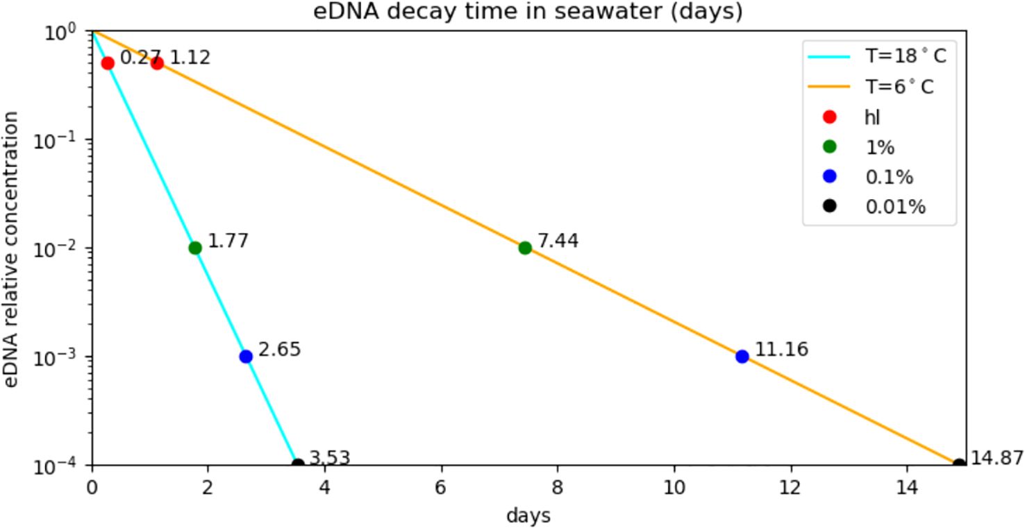
Figure 1. Modelled decay of eDNA in seawater (Equation 1) for seasonal minimum (6°C) and maximum temperatures (18°C) for the study area. The points show the effect on eDNA longevity in the model from selecting different minimum relative detectable concentrations, starting with half-life (hl), or 50%, to 0.01% of the source concentration. By reducing the threshold concentration 10x (e.g from 1% to 0.01%) the life of an eDNA in the model is extended by a constant value of 21h07m (3d17h) at 18°C (6°C).

The higher the concentration of eDNA the more likely it is to be detected. Even if the transport, and resulting dilution, and the biological decay are perfectly represented in the model, two terms are undefined: the concentration at the source and the minimum detectable concentration. eDNA concentration at source will depend on species (shedding rate) and the mass of source organisms (Andruszkiewicz Allan et al., 2021; Sansom and Sassoubre, 2017; Sassoubre et al., 2016). The detectability limit again varies with the details of the assay (e.g. sampling volume, metabarcoding vs. qPCR). Davison et al. (2019) and Ellis et al. (2022) found different detection and quantification limits for different species.

To keep the simulations as general in terms of species being detected and methods being used, we defined an arbitrary eDNA detection limit: a threshold of 0.01% of the source concentration (i.e. decrease by 10,000x) below which eDNA was considered undetectable, and tracking of trajectories was stopped. This is a cautious approach as the ratio of typical eDNA concentrations at the source to the limit of detectability using qPCR is around 10x. Concentrations of eDNA at the source are likely to vary greatly with species and behaviour but examples from the bibliography are 535 and 120 copies/L for flounder and stickleback (Thomsen et al., 2012) and 263 copies/L for shore crab (Collins et al., 2018). By including a study on Cod (Salter et al., 2019) the detection limit covers a range of 48 to 83 copies/L, resulting in a ratio of less than 10x. By tracking parcels through a 10,000x decrease we are allowing for larger sources concentrations and improved limit of detection. As the likelihood of detection is given by the decay in concentration from source to detection, the resulting maps and distance statistics are mostly unaffected by the very low concentrations of long-lived trajectories. Figure 1 shows the modelled persistence of eDNA for winter and summer, for several values of relative detection concentrations from 50% to 0.01%.

2.3 Hydrodynamical forcing fields and drifter trajectories

Modelled trajectories were validated against observed trajectories from drifters attached to a drogue. These were drifters deployed by Cefas (Hill et al., 2008) covering the period 1995 to 2003.

The OceanParcels model was forced by output from the NEMO model in the Atlantic Margin 7 km configuration (AMM7) (O’Dea et al., 2017). Direct model output was provided by the MetOffice through request and covered the years 2000-2012. The output is in terrain following coordinates and includes vertical diffusivity (variable avm in the model) which was required to parameterise turbulence in the 3D simulations. AMM7 direct output wasn’t available to compare against trajectories before 2000, and so publicly available AMM7 outputs distributed by Copernicus Marine services (CMEMS) (doi:10.48670/moi-00059) were used. These are in z vertical coordinates and don’t include vertical diffusivity, which wasn’t required for reproducing surface drifters.

2.4 Model experiments

Four sets of experiments were undertaken: i) calibration and validation, using only currents for the depths of Cefas drogued drifters (20 m), ii) sensitivity analysis, for estimation of the number of parcels to release per location, iii) effect of surface/seabed release and iv) realistic 3D simulations of eDNA dispersal (see Table 1 for more details). The realistic 3D simulations included both seasonal and interannual variability. The months of January and July were selected to represent the annual extremes in water temperature and thus in decay rates, and to represent both winter and summer wind conditions, which will affect the advection of parcels near the surface. The wind patterns also change from year to year and the North Atlantic Oscillation (NAO) monthly index was used to select 3 particular months of January and July in the range 2000–2012 with low, medium and high windiness values (Table 2).

Table 1

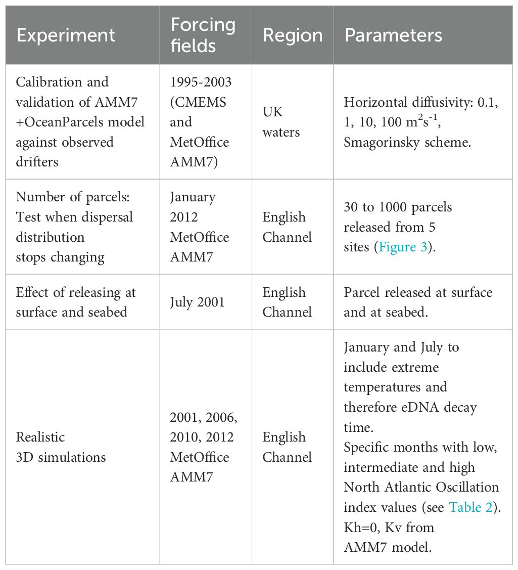
Table 1. Description of OceanParcels simulations.

Table 2

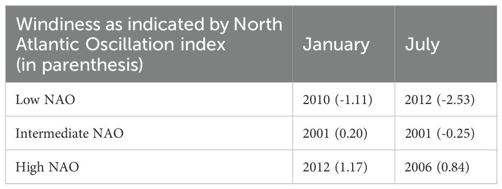
Table 2. Month and year combinations selected to capture different water temperatures, and low, intermediate and high North Atlantic Wind Oscillations (NAO).

2.5 Calibration and validation against observed trajectories

Usually, observed trajectories in the sea come from drifters at the surface, as it is very difficult to determine the horizontal position of a drifter at depth. The modelled ocean currents and the OceanParcels advection-diffusion solution was validated by comparing against drogued drifters, which hang 20 m below a surface buoy. Therefore, only validation of near-surface movement was possible.

The validation was done in three successive steps as illustrated in Figure 2. First, 12 drifter trajectories that serve as observations were selected from across the UK and split into two evenly distributed subsets of 6. Then the horizontal diffusivity coefficient, K_h that best matched the observations was selected (calibration step) using the first subset. Using the second subset, model runs using the selected parameters were compared against a different set of trajectories to allow the trajectory error to be quantified (validation step).

Figure 2

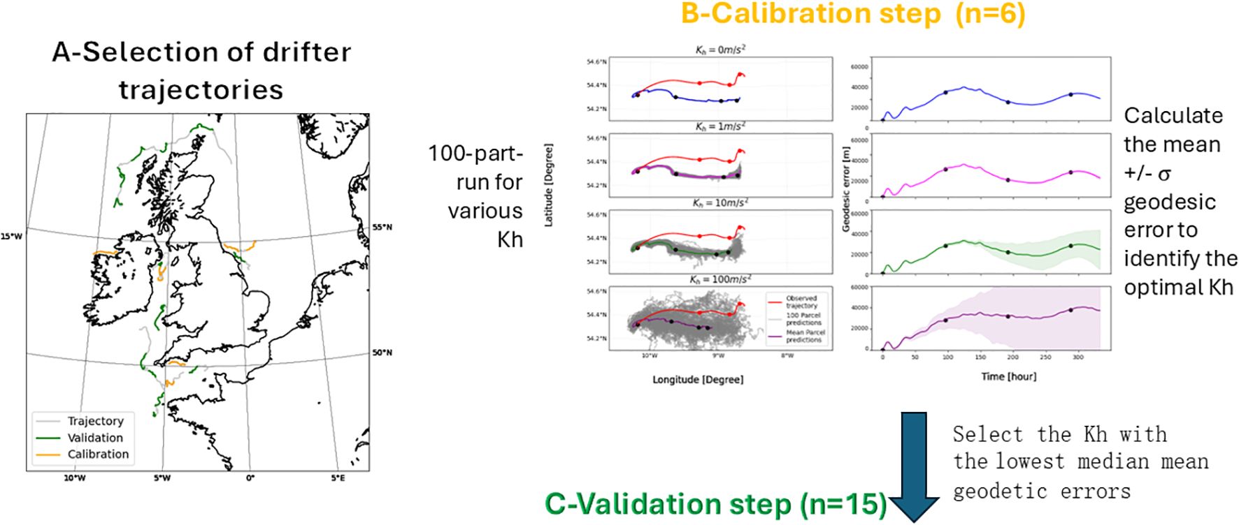
Figure 2. Three steps model validation process. In the calibration step 2B the solid dots mark 4-day-time stamps to ease the comparison between the error plot (right) and trajectory plot (left). Kh is horizontal diffusivity.

2.5.1 Selection of drifter trajectories

Drifter trajectories were selected according to location (over the North West European shelf, preferably near the coast), duration (minimum 2-week-long due to eDNA decay rate, see Figure 1) and continuity in the data (no gaps). Among the 12 selected drifters in UK waters, 4 were in the English Channel waters, where the main eDNA simulations were focused.

As the maximum eDNA lifespan was calculated as 14 days, we extracted 14-day-long sub trajectories from the drifter trajectories to calibrate (orange) and validate (green) the OceanParcels model (Figure 2). This maximises the number of trajectories available and ignores the cumulative error for runs longer than 14 days. The number of sub-trajectories varied between 1 and 6. The 6 drifter trajectories used for validation comprises 12 sub-trajectories (Supplementary Figure 1, Supplementary Table 1). Further information on the sub-trajectories release location and dates, and use in calibration or validation, can be found in Supplementary Figure 2 and Supplementary Table 2).

2.5.2 Calibration of horizontal diffusivity, K_h

Turbulent eddy processes in the ocean, that are too small to be represented in the hydrodynamical model grid, can be introduced in the trajectory solution through the use of tracer diffusivity parameterisations (Reijnders et al., 2022). The most common form is a random walk model, which is equivalent to diffusion in Eulerian models (van Sebille et al., 2018). Since the 7 km ocean hydrodynamical model used here is mostly eddy resolving (O’Dea et al., 2017), we compared using advection alone, with advection-diffusion using various values for horizontal diffusivity and the Smagorinsky scheme, which dynamically estimates K_h from horizontal velocity shear stress. A rough estimate of the value of horizontal diffusivity, K_h, can be obtained from Stommel’s 4/3 law of oceanic diffusion (Schönfeld, 1995):

$$K_h=K_0{(\frac{l}{l_0})}^{\frac{4}{3}}$$

where l is the length scale and l₀ a reference length scale of 1 km. From diffusion experiments in the North Sea covering length scales between 1 and 5 nm (see references in Schönfeld (1995)) the constant K₀ is set to 1.1x10–⁴ m^2/3 s^-1. Setting l=7 km from the resolution of the AMM7 forcing fields, K_h = 10 m² s^-1. Therefore, we decided to test K_h values of 0, 1, 10 and 100 m² s^-1 to be sure to cover a wide range. As presented in the trajectory plots in Figure 2 (B-Calibration), an increasing in horizontal diffusivity coefficient, K_h results in a spreading of eDNA trajectories (100 grey trajectories) and a faster mean displacement (dots along the coloured mean trajectory displayed every 3 days are closer) and the standard deviation of the error is wider.

Several advection-diffusion numerical schemes are available in the OceanParcels model. We used the Milstein Advection-Diffusion scheme of order 1 (hereafter M1) when applying a constant horizontal diffusivity, as it is efficient computationally and is a default choice in OceanParcels (https://docs.oceanparcels.org/en/latest/examples/tutorial_diffusion.html). When not using horizontal diffusivity the Runge-Kutta 4^th order numerical scheme for advection was selected, (noted RK4_2D and RK4_3D in 3D). Additionally, the Smagorinsky scheme, noted smag, was also used, with a standard coefficient value of the coefficient C_S=0.1. This estimates the value of K_h locally from velocity shear stresses.

The metric used to quantify the error in the simulated trajectory compared to the drifter’s trajectory (observation) is the geodesic distance, or the shortest distance between the two trajectories on the surface of the geoid. This was calculated for each trajectory time-step and then averaged in time. As the selection of the best numerical scheme requires the calculation of geodesic distances between two trajectories, the median of the errors for 6 observed tracks was calculated.

2.5.3 Validation

The validation attempts to reproduce a separate set of 12 sub-trajectories using the calibrated value of K_h. Similarly to the calibration, the quantification of error uses the geodesic distance calculated between the mean model prediction and the drifter trajectory. Similarly to the calibration subset, validation trajectories are from across UK waters, encountering diverse hydrodynamic conditions. Amongst the twelve 14-day-long sub-trajectories, five trajectories were present in the English Channel waters.

2.6 Sensitivity to number of release events per location

The main experiment aimed to assess the range of eDNA dispersal distances under a full neap-springs tidal cycle (approximately 14 days) and for this, parcels were to be released at regular intervals. The higher the number and frequency of releases, the better the estimate of dispersal distance, but also the higher the computational cost. In this sensitivity study five experiments were conducted, with 30, 100, 300 and 1000 releases per location over the 14 days neap-spring cycle, resulting in releases at intervals of 10.2 hours (for release of 30 parcels) down to 20 minutes (for release of 1000 parcels). Also, parcels were released from five locations with contrasting tidal conditions (see Figure 3 and location details in the Supplementary Material, Table 4).

Figure 3

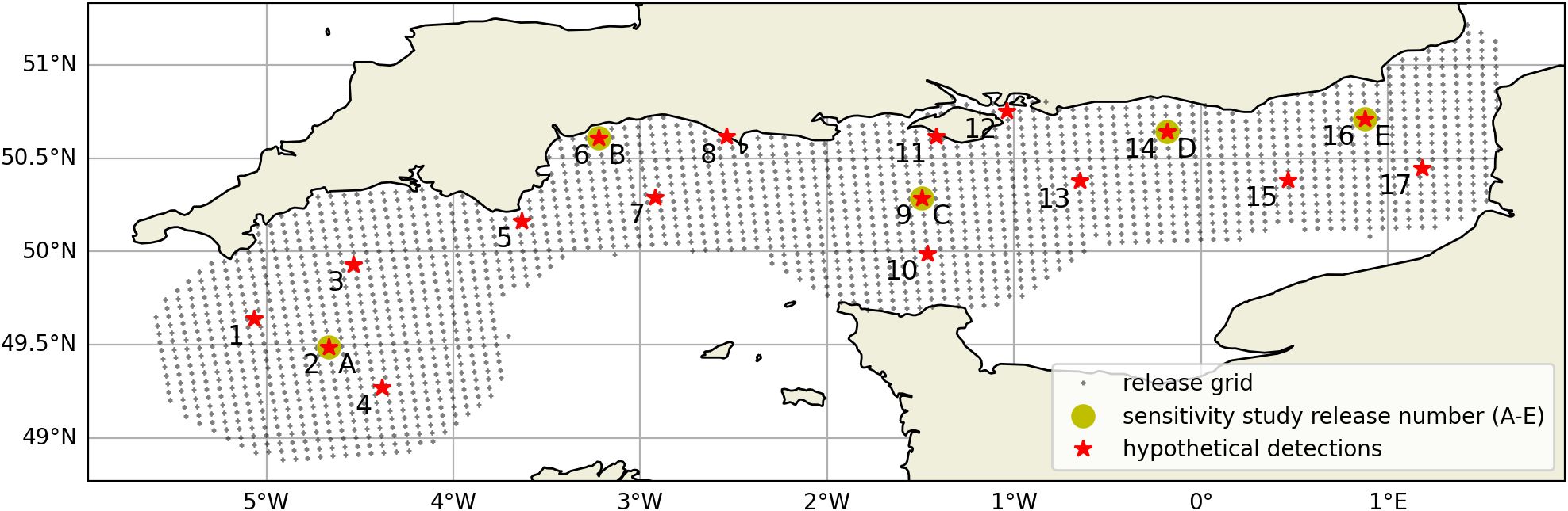
Figure 3. Map of the English Channel showing the 17 hypothetical eDNA detection locations (red *) and release grid (+) used for the backtracking method. The filled yellow circles labelled A-E indicate the 5 locations used in the sensitivity study on number of releases. Locations are detailed in the Supplementary Material Table 4.

A sufficient number of releases per point was selected when no difference was visible in the frequency distribution of dispersal distance by increasing number or releases. The dispersal distance was assessed using two metrics: the geodesic distance to origin, and the geodesic distance to the centre of mass of all the parcels for each moment in time.

2.7 Effect of release depth

The NEMO AMM7 model used to provide the 3D currents and vertical diffusivity for OceanParcels, is able to represent vertical stratification in summer (O’Dea et al., 2017). At depths where sharp changes in vertical density gradients take place, the low turbulence at the pycnocline can act as vertical barriers to mixing. Parcels released above the pycnocline will have difficulty in crossing underneath, and vice versa. The effect of the release depth was tested by releasing 100 parcels at the seabed and at the surface on the 1^st of July 2001, at two locations: i) a seasonally stratified site just East of the Isles of Scilly (50.0N, 6.2224W) and ii) a well-mixed site in the Eastern Channel (50.377°N 0.647°E). The stratified site was chosen as to be west of the position of the Ushant Front, which is the name given to the oceanographic feature separating these two regimes in Summer (Pingree, 1975).

2.8 Pseudo-backtracking

For the main experiment, 17 locations were selected as the sites of hypothetical eDNA detections (Figure 3; Supplementary Material Table 4). The backtracking of the parcels to determine the source location is complicated by the presence of diffusivity in the mathematical solution. In this case the trajectory can’t simply be solved backwards in time as this will differ statistically from the forward trajectory (Thygesen, 2011). Here we used a pseudo-backtracking method as in Andruszkiewicz et al. (2019) by releasing parcels at regular time intervals (see Table 1) over a regular grid of 5 km (see Figure 4 for a visual explanation of the method). During the simulation the parcel position and relative concentration are recorded every hour. Tracks that pass within a certain radius of the detection location are marked as possible eDNA sources including all past locations (Figure 4A); the radius was set to 10.5 km which is 1.5 time the resolution of the AMM7 model to make sure that the complete cell was always included. For each past position the relative reduction in concentration until reaching the target is calculated (Figure 4B). These positions and modified concentrations (Figure 4C) are interpolated to generate a 2D probability density of origin (Figure 4D).

Figure 4

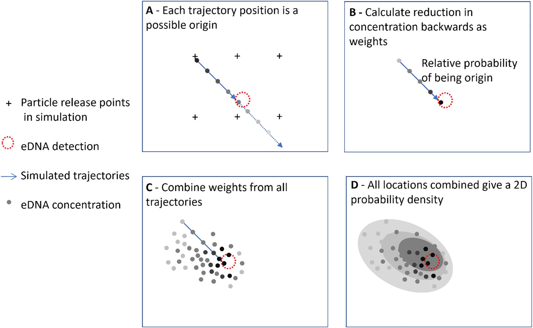
Figure 4. Explanation of the pseudo backtracking method used to determine probability of origin. Trajectories start at regular grid points and propagate forward in time; trajectories that pass within a radius of the eDNA detection point are treated as representing the possible sources. Darker shading depicts higher eDNA concentration and higher probability of origin.

2.9 Explanatory variables driving dispersal

Conditional Random Forest regression models were used to infer importance of 6 variables in predicting the pseudo-backtracked eDNA dispersal distances. The independent variables were year, month, NAO, distance from coast, tidal excursion, and depth. Separate models were built using the median distance and 95^th percentile distance as responses. The procedure used follows that of Strobl et al. (2009) and was implemented in R version 4.2.2 using the cforest() function of the party package version 1.3-15 (Hothorn and Zeileis, 2015).

Random Forest is a robust machine learning algorithm that makes no linear assumption on the relationship between response and explanatory variables and consists of resampling the underlying dataset multiple times and building a decision tree from each sample (number of trees = n_trees), followed by aggregating the results. Each tree is built by randomly selecting a subset of variables at each node (number of variables chosen = m_try) to form a subset from which the best splitting variable is chosen such that splitting the data into two groups minimises the sum of squared residuals. This splitting process is repeated until a minimum number of observations is achieved at the end of all the branches. To avoid variable-selection bias, i.e. bias towards continuous variables and factors with many levels, unbiased decision trees were used as base learners (Hothorn et al., 2006; Strobl et al., 2007). Conditional permutation, which accounts for correlations among variables was used to determine variable importance (Strobl et al., 2008). For each model, 50 permutations were used to obtain a measure of uncertainty for the permutation-based variable importance.

Models were built to explain the median and the 95^th percentile of the geometric distance from source. Both models used default initial n_trees= 500 and m_try = 5. Repeated 10-fold cross validation was conducted on the entire dataset using the train() function of the ‘caret’ package version 7.0-1 (Kuhn, 2008) to assess model performance and tune hyperparameters. Ten repeats were used, and the average root mean square error (RMSE) calculated while searching across a grid of m_try from 1 to 5. Tuning of this hyperparameter suggested that using m_try = 5 yielded the lowest averageRMSE i.e. best performance in both models, so subsequent inference was based on this value.

3 Results

3.1 Calibration and validation of the trajectory model against drifter trajectories

Calibration results are presented in orange in Figure 5, for fixed values of K_h between 0 and 100 m²s^-1 and for the Smagorinsky scheme. Supplementary Materials Table 2 and Figure 4 shows the mean geodesic error for the full trajectory, against 6 drifters. K_h=1 was selected for the validation as it had the lowest error (median=4,333 m, n=6). Figure 5 in blue shows the spread and median of the geodesic error when the 15 validation sub-trajectories were reproduced using the selected value of K_h (median=6,827 m). Details in geodesic errors for the 15 validated sub-trajectories are provided in Supplementary Table 3.

Figure 5

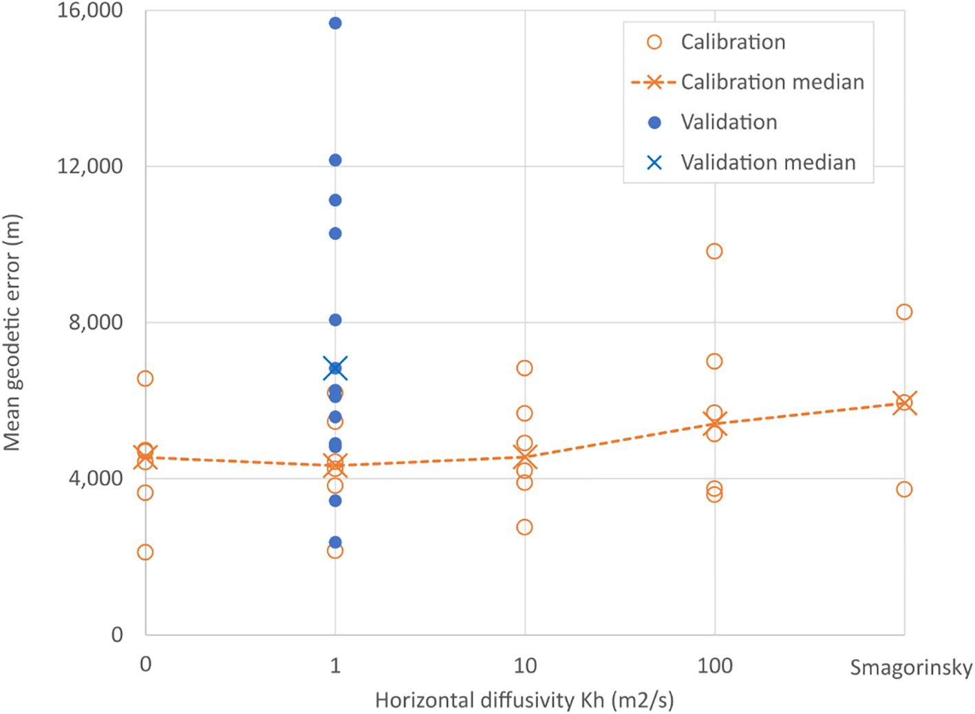
Figure 5. Error of simulated trajectories when compared with drifter tracks. Calibration of the horizontal diffusivity, K_h, led to the selection of a value of K_h=1m²s^-1 as it had the lowest error. Trajectories run with this value were then compared with the validation dataset resulting in a median geodetic error of 6,827 m.

3.2 Sensitivity to number releases per location

Figure 6 shows the empirical probability distributions for two measures of dispersal: distance to origin and distance to centre of mass. Results for 30 releases are visually noisier, but from 100 releases upwards the distributions are visually similar. This frequency corresponds to a release every 3h21m. Below a certain number of releases, or equivalently above a certain time between releases, the tidal forcing is being subsampled, and it is not possible to capture all the variability in the forcing. The main eDNA simulations were conducted using this value of 100 releases per site over a neap-spring cycle.

Figure 6

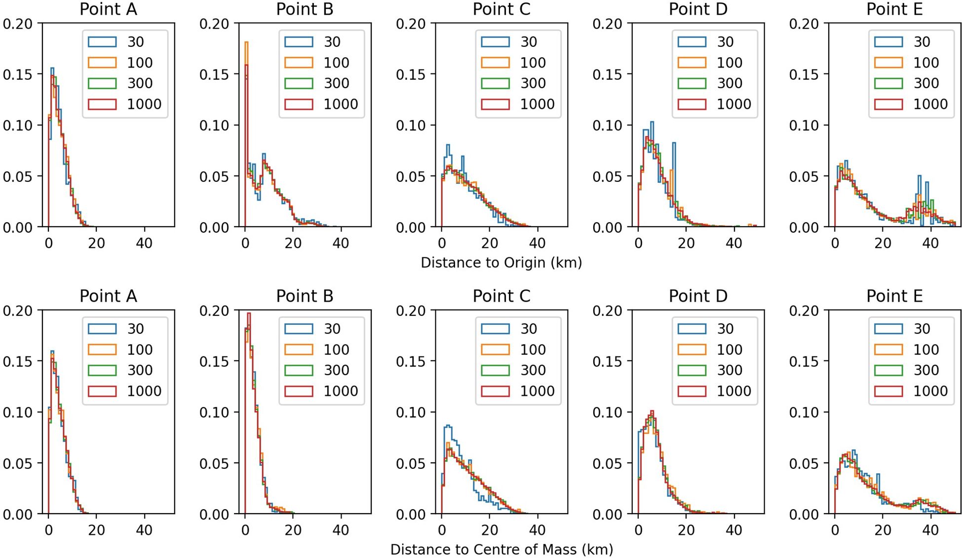
Figure 6. Distribution probability of dispersal distance, for different numbers of releases per location. Top row has distance to origin and bottom row, distance to the centre of mass of all positions. The location of point A to E are shown on Figure 3. There is little visual difference in the dispersal distance distribution for 100 releases per location or more.

3.3 Effect of release depth

Figures 7 and 8 show the horizontal and vertical dispersal of each parcel released from the two selected sites. At the stratified site the direction of dispersal differs with release depth, with surface parcels moving further to the South-East, although with similar dispersal distances (Figure 7). The existence of a thermocline between 10 and 40 m results in a minimum of vertical diffusivity which explains reduced mixing between surface and deeper waters. At the well mixed site, the vertical distributions quickly become independent of the release depth as vertical diffusivity is much higher and peaks at mid depth (Figure 8).

Figure 7

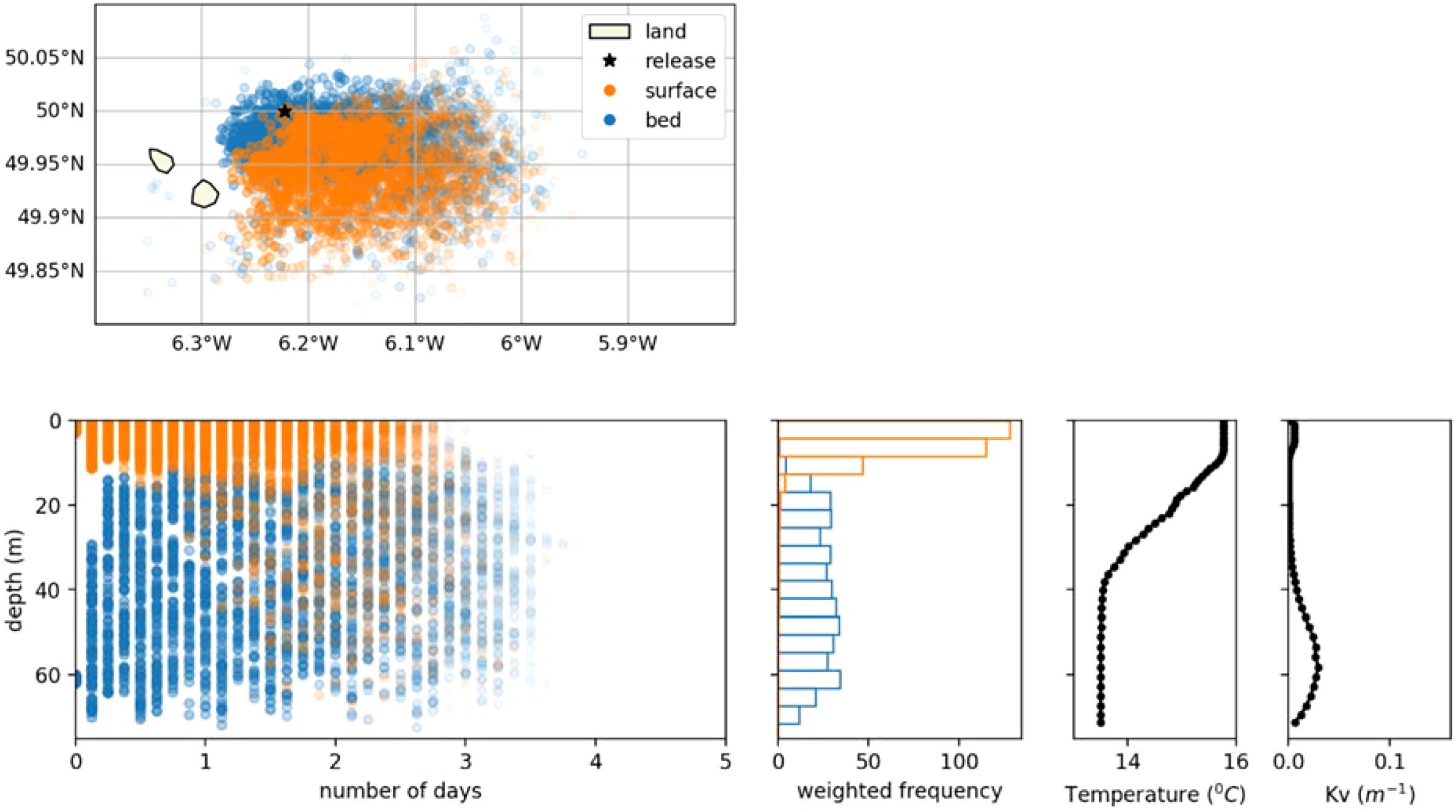
Figure 7. Effect of release at surface vs. at seabed in a seasonally stratified location off the Isles of Scilly (50.0°N 6.222°W, released on 1/7/2001). Top: map view of likelihood of origin. Bottom row (left to right): likelihood of origin for time and depth, vertical distribution of likelihood of origin over 5 days, temperature and vertical momentum diffusivity from the NEMO model.

Figure 8

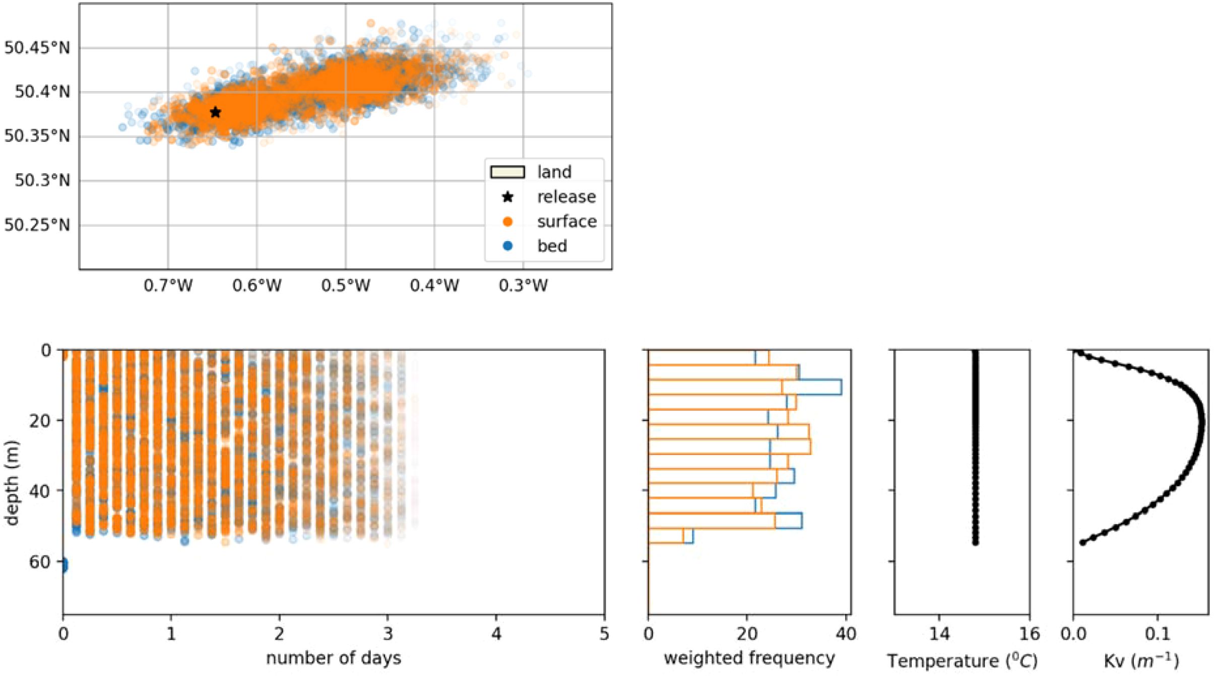
Figure 8. Effect of release at surface vs. at seabed in a well-mixed location in the Eastern Channel (50.377°N 0.647°E, released on 1/7/2001)). Top: map view of likelihood of origin. Bottom row (left to right): likelihood of origin for time and depth, vertical distribution of likelihood of origin over 5 days, temperature and vertical momentum diffusivity from the NEMO model.

3.4 Realistic 3D simulations

Six different environmental scenarios were simulated incoporating combinations of summer, winter and three NAO conditions. The likelihood of origin is mapped for two of these scenarios representing summer and winter conditions (Figure 9, for the remaining maps see Suplementary Material). The area around hypothetical detection sites, representative of eDNA dispersal distance, is generally larger under Winter simulations compared to Summer simulations.

Figure 9

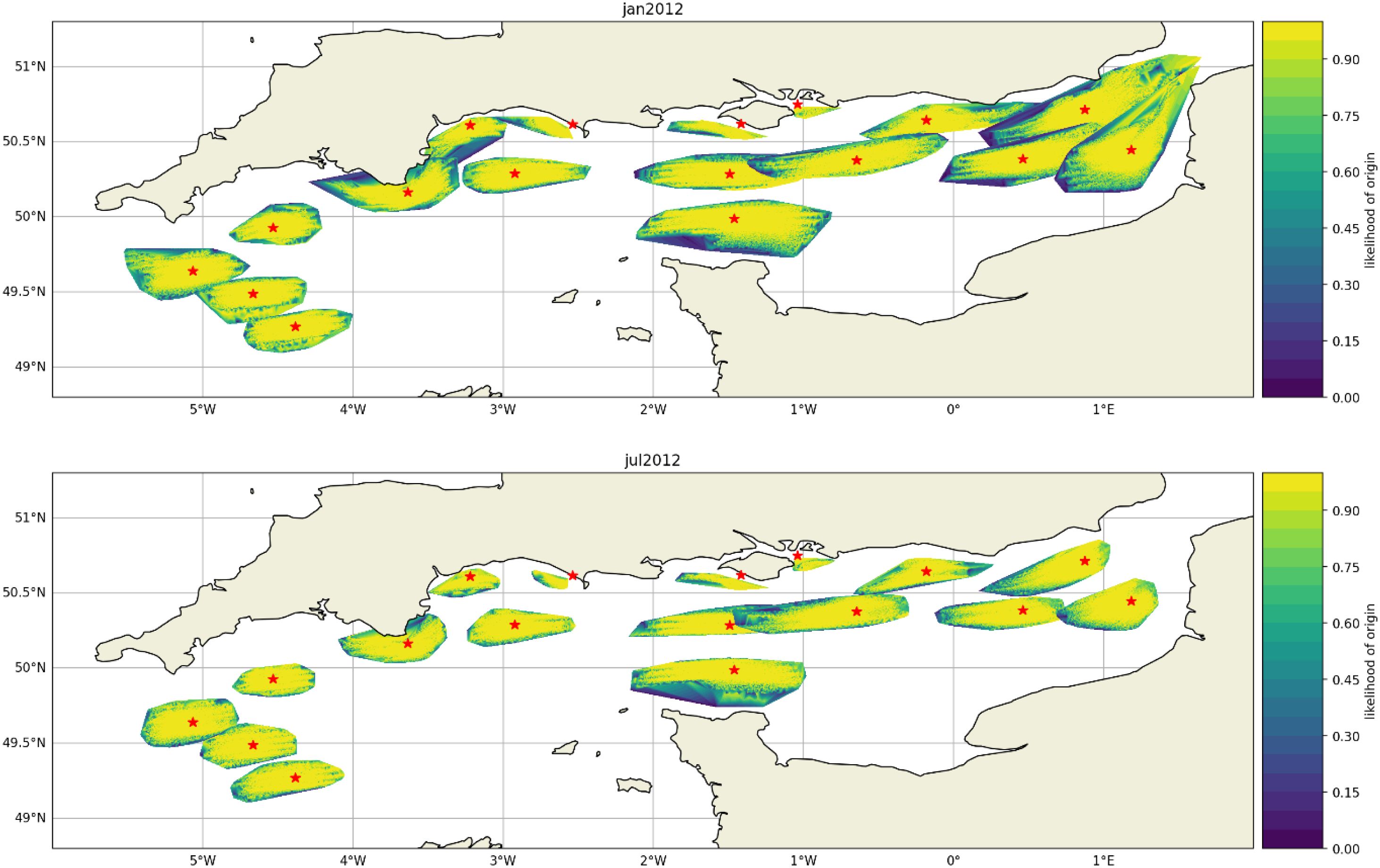
Figure 9. Likelihood of origin for eDNA detected at the 17 hypothetical sites (star) for January (top) and July 2012 (bottom) in the English Channel. The polygons representing distance to origin are larger in January than July due to slower eDNA decay in colder water.

Figure 10 shows the cumulative distribution of the source likelihood integrated along distance to source. The median distance was 7.61 km while the 95^th percentile was 18.57 km. Separating the results between Summer and Winter the average of the typical (median) distance to source was 7.03 and 8.27 km respectively.

Figure 10

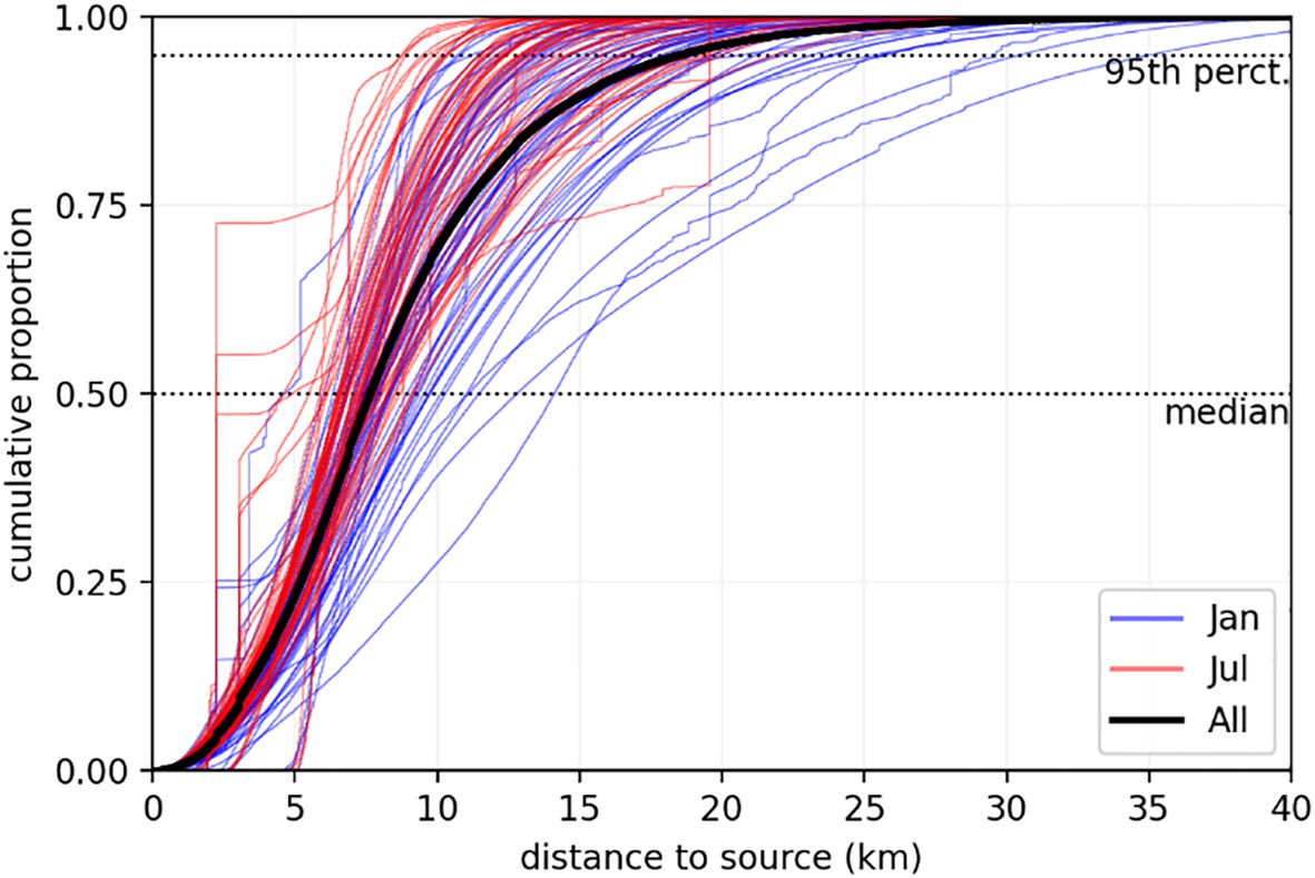
Figure 10. Cumulative distribution of the distance to source for the 17 sites and 6 seasons, coloured by month. The thick black line represents the distribution for all sites and experiments.

In Figure 11 the two distances to source – median and 95^th percentile – are plotted against 6 of the environmental factors. Two of these, tidal excursion and month, have significant statistical relationships with distance to source. Tidal excursion has a linear relationship (p<0.001) with both distances. Also, there was a significant difference in both the median and 95^th percentile of distance to source (p<0.001) between the month of January and July.

Figure 11

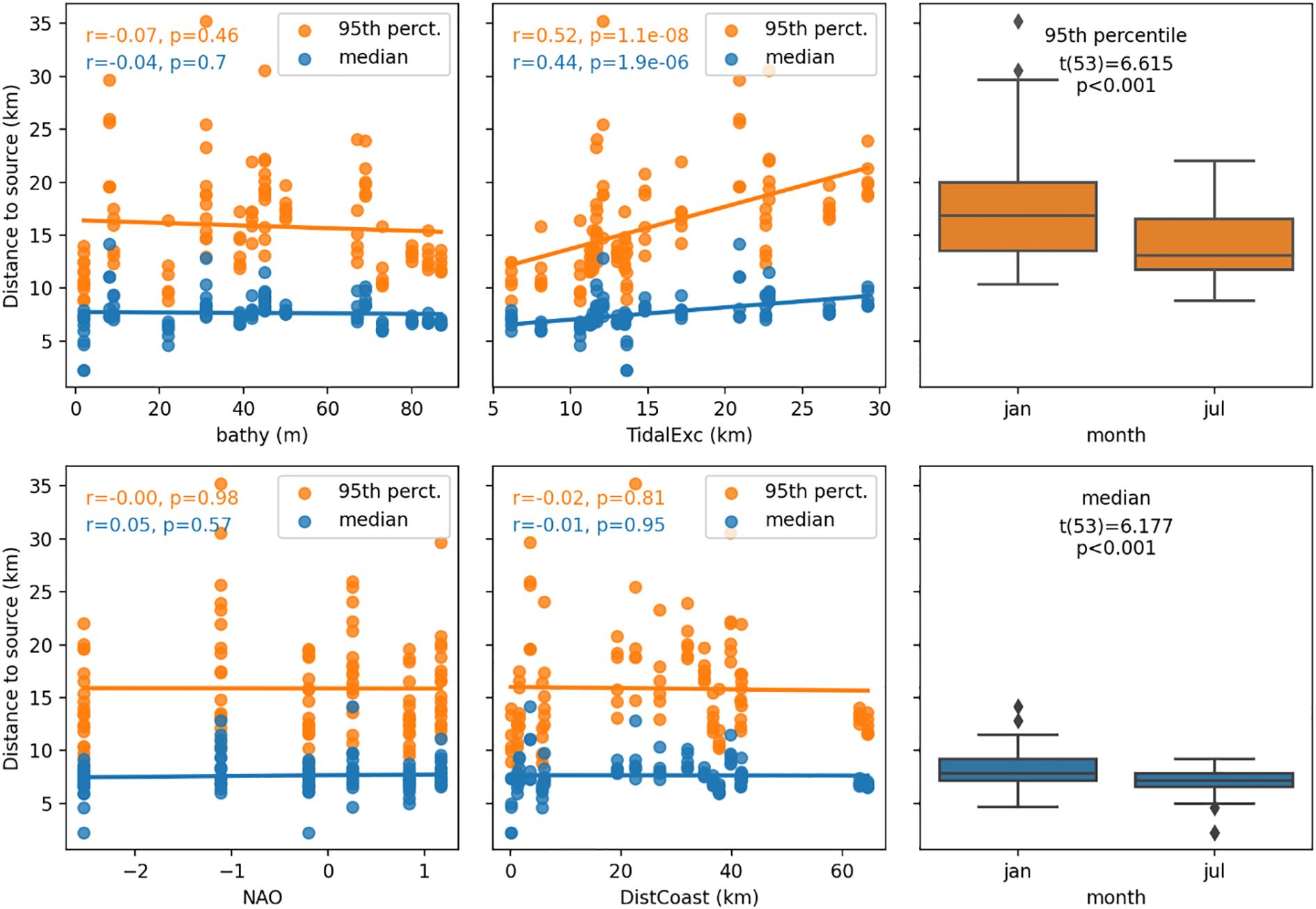
Figure 11. Relationship between environmental factors and both median and 95th percentile of distance to source. Note that tidal excursion (TidalExc) has a significant linear relationship with both median and 95^th percentile of the distance-to-source (p<0.1%). Results of paired t-test are reported on the boxplots for variable month.

3.5 Explanatory model

For the median distance to source, repeated cross-validation yielded average RMSE=1.21 km and R² = 0.49 on the best model. Conditional permutational importance was highest for tidal excursion and month with comparatively little importance ascribed to any of the other variables (Supplementary Materials Figure 6a) and these two variables were included in the majority of conditional decision trees (Supplementary Figure 6b). The selected variables were the same for the 95^th percentile of the distance to source but with RMSE=3.52 km and R² = 0.52, and with even lower relative importance for any of the other variables (Supplementary Figure 7a). These two variables were included in the vast majority of conditional decision trees (Supplementary Material Figure 7b).

4 Discussion

The exercise to calibrate the horizontal diffusivity, showed best matches to the drifter-buoy trajectories for Kh=1, followed by 0 and 10 m²s^-1. Kaandorp et al. (2020), considered the same range of K_h values when calibrating 2D litter simulations on a model with similar resolution (1/16 deg.) and following comparison with the results of an inverse model fitted to tracer statistics, selected Kh=10 m²s^-1 but saw very similar results for K_h=1 m²s^-1. The validation, using Kh=1 m²s^-1, demonstrated the suitability of the modelled currents to reproduce the observed trajectories over a period of 14 days (limited by eDNA decay in the ocean). The median error along the trajectory was just under the model resolution of 7 km.

Unlike the subsurface drifter-buoy trajectories used in the calibration, the main eDNA simulations parcels move in 3D. Best practice is to represent vertical movement a as vertical random walk, with the vertical diffusivity being provided by the hydrodynamical model (van Sebille et al., 2018; Visser, 1997). It was decided not to include additional horizontal diffusivity (K_h=0) as the calibration showed that lower values of horizontal diffusivity performed better than high values. Another reason to have Kh>0 is to add a stochastic behaviour to the model to represent uncertainty, and this was already enabled by the inclusion of vertical diffusivity.

The experiment of the effect of the release depth showed conditions and time scales when it matters that eDNA is sampled across a pycnocline from where it was shed, for instance benthic species sampled at the surface or surface species sampled at depth. For a well-mixed water column, such as seen during winter on the continental shelf, releasing at the surface or at depth didn’t result in a difference in eDNA concentration with depth. On the other hand, for the Summer stratified conditions, which are seen in much of the European shelf between March and October (van Leeuwen et al., 2015), the thermocline impairs mixing and it takes several days for the concentration of eDNA to become comparable, by which time it has greatly degraded, reducing the probability of being detected.

Backtracking analysis of the realistic experiments in 3D show that the distance to the source varies greatly with location and month: Figure 10 shows the median distance to vary between 2.5 and 15 km and the 95^th percentile to be as high as 40 km, with an overall median of 7.61 km and 95^th percentile of 18.57 km.This goes against the initial assumption in marine eDNA that it would only represent very local conditions (Foote et al., 2012) or that the decay only affects persistence time and sampling frequency, without considering the possiblity that the eDNA was shed at a distance from the source (e.g. Barnes et al., 2014).

According to the explanatory model, the most important factor in explaining the variation in distance accross the region and for the six environmental scenarios, is tidal excursion at the site of detection. The English Channel experiences strong tides with tidal excusion at the sites considered varying between 6 and 29 km. The second factor was month (January/July to represent winter/summer) wich will differ in water temperature and as a result in eDNA decay. It is also likley that eDNA dispersal is increased by enhanced density and wind driven transport in winter (Holt and Proctor, 2008).

4.1 Implications for sampling and monitoring

Decay of eDNA with time is seen as both a source of false negatives, such as when sampling is not frequent enough, or of false positives, for instance when transitory individuals can’t be separated from local populations (Troth et al., 2021). Additionally, transport of eDNA by water, can be seen as both a source of false negatives and false positives. The former can be when locally shed DNA is diluted and transported away, for instance, in rivers the probability of detection can increase away from the source (Wood Z. T. et al., 2021). One example of false positive is the detection of a riverine species downstream in a lake (Jo and Yamanaka, 2022).

An accurate description of both decay, transport and mixing, as what was attempted here for the English Channel, can be used to design sampling to fit the intended species and usages. In the simulations, an eDNA detection in East of Start Point MPA (point 8 in Figure 3) in January can be from a source as far as 30 km to the west, 15 km East or 5 km North of South. The half-time of eDNA at 6 deg. C is 1.12 days, which we can interpret as an approximate median age of eDNA detected. The explanatory model shows that local average tidal excursion is the main control of distance to source, but it can also be inferred that selecting the state of neap-spring cycle it is possible to shape the sampling area. As an extension of this, for fast degrading conditions experienced in July, choosing high slack tide in the English Channel will favour a detection from the West, and vice versa for low slack tide.

As shown before, the depth of the sampling should take into account the presence of a pycnocline and the depth at which the shedding is expected to happen, otherwise the risk of false negatives increases.

In the present analysis the full range of neap-spring conditions were taken into account to represent the full range of origins for each eDNA detection location. The same method can be applied to actual survey detections at a specific moment in time, which will correspond to a state of the tide and wind. The estimate for the likelihood of origin is likely to be less symmetrical than those shown in Figure 9 being strongly weighted by the state of the tide in the hours preceding the observation.

4.2 Range of distances in the context of published results

To put range of modelled eDNA spatial bounds in the context of previous observations and simulations, we surveyed published estimates of eDNA dispersal distances for both freshwater and marine environments. Since eDNA transport and degradation differ with the environment, Harrison et al. (2019) recommended to categorise reported distances by ecosystem type (lentic, lotic, and marine). Figure 12 shows dispersal distances reported for different ecosystem types, distinguishing between those simulated by models and those observed in the field. Within each type, the studies are sorted by year to show the evolution of estimates. For both lotic freshwater and marine environments, modelled maximum dispersal distances were larger than observed in the field. The results in the present study are within the range of previous studies using marine models which included eDNA decay (Andruszkiewicz et al., 2019; Ellis et al., 2022), but up to one order of magnitude above the maximum distances observed in the ocean (Ellis et al., 2022; Kutti et al., 2020). It is worth noticing that while modelled maximum dispersal estimates have coalesced around 10km, observed studies have increased 3 orders of magnitude since Foote et al. (2012), possibly showing improvements in detection and study designs that sample further away from natural or manipulated eDNA sources. For freshwater lotic, distances above 10 km have both been observed (Deiner and Altermatt, 2014) and modelled (Pont et al., 2018), but generally the dispersal distances observed are smaller than those modelled. Ellis et al. (2022) was able to compare modelled distances with observations for two species in the marine environment, and also reported larger distances from simulations. This was attributed to: optimistically slow modelled decay, insufficient temporal variability in the model, and the difficulties involved in detecting low eDNA concentration patches in situ. In the present study the modelled decay tries to be more realistic by taking into account the varying water temperature in the 3D model. As it is based on experiments in the lab and in mesocosms, it could still be that these didn’t include important processes that accelerate decay in the environment such as UV light, turbulence or different microbial community (Barnes et al., 2014).

Figure 12

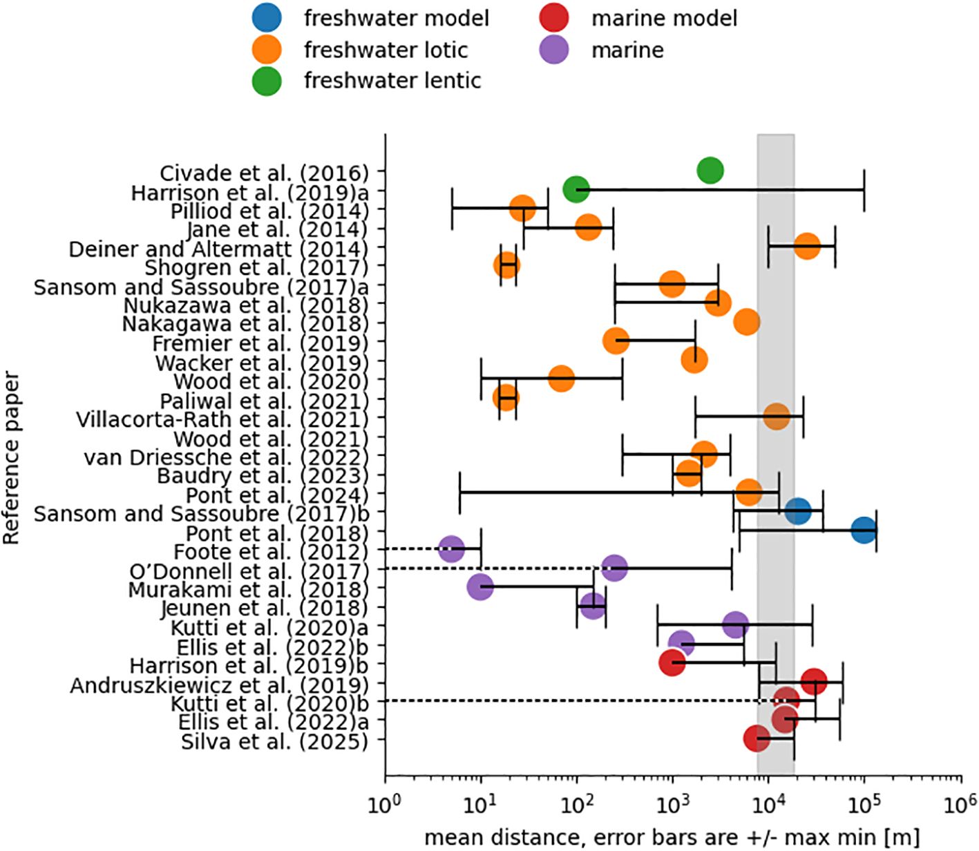
Figure 12. eDNA travelled distances reported in published papers and classified by environmental mechanistic process. The mean travelled distance is symbolised with a coloured dot and associated black error bar indicates the maximum and minimum travelled distance. Dotted lines point to a minimum distance of 0m (the source). The shaded area covers the upper distance limit in this study. When distances were reported for two different environments in the same paper, reference was appended with “a” and “b”. For notes on each reference see Supplementary Materials, S3 - Notes on references from bibliography.

4.3 Factors not considered in modelling approach

While recent modelling studies, such as this, have improved the representation of eDNA decay in the ocean, the limits of detectability of molecular techniques have yet to be incorporated. We used an arbitrary eDNA detection limit of 0.0001 of the original concentration for halting trajectory calculations, same as used by Ellis et al. (2022). When calculating likelihood maps or distance distributions, the concentration and dilution are used as weights, thus the median and 95% percentile of the distance becomes less sensitive as concentrations reduce. Nevertheless, the limit of detection (LOD) of the eDNA methodology in use for each particular case is not being considered, which would better allow to determine the maximum dispersal distances (the perimeter of the likelihood polygons). A further unknown is concentration of eDNA at the source which depends on the species shedding rate and size of the population (both number and size of individuals). Unless this is known, the distance estimate will carry this uncertainty, that is, the eDNA detection might have been the result of a small source nearby or a larger source further away (within the constraints of currents and decay).

To enhance the accuracy of eDNA modelling, future efforts should include controlled release experiments and targeted field surveys. These initiatives will help calibrate and validate the added complexities in the models, such as variations in microbial communities and their impact on degradation rates, the different states of eDNA (particulate, intracellular, and dissolved), and the shedding rates influenced by life cycles and behaviours. Additionally, incorporating diverse environments like estuaries and deep-sea habitats will further improve the models’ applicability and usefulness”.

Conclusions

This study improves the evidence to inform our understanding of eDNA dispersal in the marine environment, which in turn enhances the accuracy with which eDNA monitoring data can be interpreted. In particular, the study highlights that eDNA data needs to be considered with environmental conditions in mind.

The study’s results can inform monitoring programmes by guiding sample spacing, optimizing sampling locations and depths, and accounting for seasonal and site-specific factors like tidal excursion and stratification.

If eDNA is to be used as a first step in detection (hierarchical methods to monitoring) of an organism, the outputs of this study facilitate a more accurate spatial targeting of traditional approaches as confirmation of species’ presence.

Ultimately this study demonstrates a methodology which can be applied retrospectively following detection of an eDNA signal. Given the temporal and regional variability of seascapes, prioritising the practical application and standardisation of methods to assess eDNA boundaries in specific contexts—rather than predefining them—will likely benefit the field the most.

Data availability statement

Publicly available datasets were analyzed in this study. The code and auxiliary data used in this study can be found https://github.com/CefasRepRes/eDNA-spatial-bound-paper.

Author contributions

TS: Visualization, Writing – review & editing, Software, Methodology, Investigation, Writing – original draft, Conceptualization. CB: Writing – original draft, Software, Visualization, Methodology, Validation, Investigation, Writing – review & editing. PL: Writing – review & editing, Methodology, Writing – original draft, Validation, Conceptualization. WR: Visualization, Methodology, Formal Analysis, Writing – review & editing, Writing – original draft. HT: Writing – original draft, Funding acquisition, Conceptualization, Writing – review & editing.

Funding

The author(s) declare financial support was received for the research and/or publication of this article. This work was funded by the UK Department for Environment Fisheries and Rural Affairs under the NIS Surveillance project and Cefas Seedcorn DP2000BJ. The research presented here used the high-performance computing (HPC) facilities at the University of East Anglia.

Conflict of interest

The authors declare that the research was conducted in the absence of any commercial or financial relationships that could be construed as a potential conflict of interest.

Generative AI statement

The author(s) declare that no Generative AI was used in the creation of this manuscript.

Any alternative text (alt text) provided alongside figures in this article has been generated by Frontiers with the support of artificial intelligence and reasonable efforts have been made to ensure accuracy, including review by the authors wherever possible. If you identify any issues, please contact us.

Publisher’s note

All claims expressed in this article are solely those of the authors and do not necessarily represent those of their affiliated organizations, or those of the publisher, the editors and the reviewers. Any product that may be evaluated in this article, or claim that may be made by its manufacturer, is not guaranteed or endorsed by the publisher.

Supplementary material

The Supplementary Material for this article can be found online at: https://www.frontiersin.org/articles/10.3389/fmars.2025.1613001/full#supplementary-material

Glossary

Backtracking: Solving trajectory of a particle backwards in time

Geodetic error: Distance measured over the surface of a geoid

Likelihood of origin: Measure of how likely a location was the source of the eDNA detected

Pseudo-backtracking: Method where multiple forward propagating trajectories are used to select trajectories that end up at target location

Pycnocline: Layer or water where there is a rapid vertical change in water density due to either temperature or salinity

Tidal excursion: Average distance water travels during a tidal cycle

References

Andruszkiewicz E. A., Koseff J. R., Fringer O. B., Ouellette N. T., Lowe A. B., Edwards C. A., et al. (2019). Modeling environmental DNA transport in the coastal ocean using lagrangian particle tracking. Front. Mar. Sci. 6. doi: 10.3389/fmars.2019.00477

Crossref Full Text | Google Scholar

Andruszkiewicz E. A., Sassoubre L. M., and Boehm A. B. (2017). Persistence of marine fish environmental DNA and the influence of sunlight. PloS One 12, e0185043. doi: 10.1371/journal.pone.0185043

PubMed Abstract | Crossref Full Text | Google Scholar

Andruszkiewicz Allan E., Zhang W. G., C. Lavery A., and F. Govindarajan A. (2021). Environmental DNA shedding and decay rates from diverse animal forms and thermal regimes. Environ. DNA 3, 492–514. doi: 10.1002/edn3.141

Crossref Full Text | Google Scholar

Ardura A., Zaiko A., Martinez J. L., Samuiloviene A., Borrell Y., and Garcia-Vazquez E. (2015). Environmental DNA evidence of transfer of North Sea molluscs across tropical waters through ballast water. J. Molluscan. Stud. 81, 495–501. doi: 10.1093/mollus/eyv022

Crossref Full Text | Google Scholar

Barnes M. A. and Turner C. R. (2016). The ecology of environmental DNA and implications for conservation genetics. Conserv. Genet. 17, 1–17. doi: 10.1007/s10592-015-0775-4

Crossref Full Text | Google Scholar

Barnes M. A., Turner C. R., Jerde C. L., Renshaw M. A., Chadderton W. L., and Lodge D. M. (2014). Environmental conditions influence eDNA persistence in aquatic systems. Environ. Sci. Technol. 48, 1819–1827. doi: 10.1021/es404734p

PubMed Abstract | Crossref Full Text | Google Scholar

Castro M. C. T., Fileman T. W., and Hall-Spencer J. M. (2017). Invasive species in the Northeastern and Southwestern Atlantic Ocean: A review. Mar. pollut. Bull. 116, 41–47. doi: 10.1016/j.marpolbul.2016.12.048

PubMed Abstract | Crossref Full Text | Google Scholar

Collins R. A., Wangensteen O. S., O’Gorman E. J., Mariani S., Sims D. W., and Genner M. J. (2018). Persistence of environmental DNA in marine systems. Commun. Biol. 1, 1–11. doi: 10.1038/s42003-018-0192-6

PubMed Abstract | Crossref Full Text | Google Scholar

Darling J. (2019). How to learn to stop worrying and love environmental DNA monitoring. Aquat. Ecosyst. Health Manage. 22, 440–451. doi: 10.1080/14634988.2019.1682912

PubMed Abstract | Crossref Full Text | Google Scholar

Davison P. I., Falcou-Préfol M., Copp G. H., Davies G. D., Vilizzi L., and Créach V. (2019). Is it absent or is it present? Detection of a non-native fish to inform management decisions using a new highly-sensitive eDNA protocol. Biol. Invasions. 21, 2549–2560. doi: 10.1007/s10530-019-01993-z

Crossref Full Text | Google Scholar

Dawson M. N., Gupta A. S., and England M. H. (2005). Coupled biophysical global ocean model and molecular genetic analyses identify multiple introductions of cryptogenic species. Proc. Natl. Acad. Sci. 102, 11968–11973. doi: 10.1073/pnas.0503811102

PubMed Abstract | Crossref Full Text | Google Scholar

Deiner K. and Altermatt F. (2014). Transport distance of invertebrate environmental DNA in a natural river. PloS One 9, e88786. doi: 10.1371/journal.pone.0088786

PubMed Abstract | Crossref Full Text | Google Scholar

Delandmeter P. and van Sebille E. (2019). The Parcels v2.0 Lagrangian framework: new field interpolation schemes. Geosci. Model. Dev. 12, 3571–3584. doi: 10.5194/gmd-12-3571-2019

Crossref Full Text | Google Scholar

Egan S. P., Grey E., Olds B., Feder J. L., Ruggiero S. T., Tanner C. E., et al. (2015). Rapid molecular detection of invasive species in ballast and harbor water by integrating environmental DNA and light transmission spectroscopy. Environ. Sci. Technol. 49, 4113–4121. doi: 10.1021/es5058659

PubMed Abstract | Crossref Full Text | Google Scholar

Ellis M. R., Clark Z. S. R., Treml E. A., Brown M. S., Matthews T. G., Pocklington J. B., et al. (2022). Detecting marine pests using environmental DNA and biophysical models. Sci. Total. Environ. 816, 151666. doi: 10.1016/j.scitotenv.2021.151666

PubMed Abstract | Crossref Full Text | Google Scholar

Fonseca V. G., Davison P. I., Creach V., Stone D., Bass D., and Tidbury H. J. (2023). The application of eDNA for monitoring aquatic non-indigenous species: practical and policy considerations. Diversity 15, 631. doi: 10.3390/d15050631

Crossref Full Text | Google Scholar

Foote A. D., Thomsen P. F., Sveegaard S., Wahlberg M., Kielgast J., Kyhn L. A., et al. (2012). Investigating the potential use of environmental DNA (eDNA) for genetic monitoring of marine mammals. PloS One 7, e41781. doi: 10.1371/journal.pone.0041781

PubMed Abstract | Crossref Full Text | Google Scholar

Gargan L. M., Morato T., Pham C. K., Finarelli J. A., Carlsson J. E. L., and Carlsson J. (2017). Development of a sensitive detection method to survey pelagic biodiversity using eDNA and quantitative PCR: a case study of devil ray at seamounts. Mar. Biol. 164, 112. doi: 10.1007/s00227-017-3141-x

Crossref Full Text | Google Scholar

Hansen B. K., Bekkevold D., Clausen L. W., and Nielsen E. E. (2018). The sceptical optimist: challenges and perspectives for the application of environmental DNA in marine fisheries. Fish. Fish. 19, 751–768. doi: 10.1111/faf.12286

Crossref Full Text | Google Scholar

Harrison J. B., Sunday J. M., and Rogers S. M. (2019). Predicting the fate of eDNA in the environment and implications for studying biodiversity. Proc. R. Soc B. Biol. Sci. 286, 20191409. doi: 10.1098/rspb.2019.1409

PubMed Abstract | Crossref Full Text | Google Scholar

Hill A. E., Brown J., Fernand L., Holt J., Horsburgh K. J., Proctor R., et al. (2008). Thermohaline circulation of shallow tidal seas. Geophys. Res. Lett. 35, 5–9. doi: 10.1029/2008GL033459

Crossref Full Text | Google Scholar

Holt J. and Proctor R. (2008). The seasonal circulation and volume transport on the northwest European continental shelf: A fine-resolution model study. J. Geophys. Res. Oceans. 113. doi: 10.1029/2006JC004034

Crossref Full Text | Google Scholar

Hothorn T., Hornik K., and Zeileis A. (2006). Unbiased recursive partitioning: A conditional inference framework. J. Comput. Graph. Stat. 15 (3), 651–674. doi: 10.1198/106186006X133933

Crossref Full Text | Google Scholar

Hothorn T. and Zeileis A. (2015). partykit: A modular toolkit for recursive partytioning in R. J. Mach. Learn. Res. 16, 3905–3909.

Google Scholar

Jane S. F., Wilcox T. M., McKelvey K. S., Young M. K., Schwartz M. K., Lowe W. H., et al. (2014). Distance, flow and PCR inhibition: e DNA dynamics in two headwater streams. Mol. Ecol. Resour. 15, 216–227. doi: 10.1111/1755-0998.12285

PubMed Abstract | Crossref Full Text | Google Scholar

Jeunen G. J., Knapp M., Spencer H. G., Lamare M. D., Taylor H. R., Stat M., et al. (2019). Environmental DNA (eDNA) metabarcoding reveals strong discrimination among diverse marine habitats connected by water movement. Mol. Ecol. Resour. 19 (2), 426–438. doi: 10.1111/1755-0998.12982

PubMed Abstract | Crossref Full Text | Google Scholar

Jo T. and Yamanaka H. (2022). Meta-analyses of environmental DNA downstream transport and deposition in relation to hydrogeography in riverine environments. Freshw. Biol. 67, 1333–1343. doi: 10.1111/fwb.13920

Crossref Full Text | Google Scholar

Kaandorp M. L. A., Dijkstra H. A., and Van Sebille E. (2020). Closing the mediterranean marine floating plastic mass budget: inverse modeling of sources and sinks. Environ. Sci. Technol. 54, 11980–11989. doi: 10.1021/ACS.EST.0C01984/ASSET/IMAGES/LARGE/ES0C01984_0005.JPEG

PubMed Abstract | Crossref Full Text | Google Scholar

Kuhn M. (2008). Building predictive models in R using the caret package. J. Stat. Software 28, 1–26. doi: 10.18637/jss.v028.i05

Crossref Full Text | Google Scholar

Kutti T., Johnsen I. A., Skaar K. S., Ray J. L., Husa V., and Dahlgren T. G. (2020). Quantification of eDNA to map the distribution of cold-water coral reefs. Front. Mar. Sci. 7. doi: 10.3389/fmars.2020.00446

Crossref Full Text | Google Scholar

Lacoursière-Roussel A., Howland K., Normandeau E., Grey E. K., Archambault P., Deiner K., et al. (2018). eDNA metabarcoding as a new surveillance approach for coastal Arctic biodiversity. Ecol. Evol. 8, 7763–7777. doi: 10.1002/ece3.4213

PubMed Abstract | Crossref Full Text | Google Scholar

Lamb P. D., Fonseca V. G., Maxwell D. L., and Nnanatu C. C. (2022). Systematic review and meta-analysis: Water type and temperature affect environmental DNA decay. Mol. Ecol. Resour. 22, 2494–2505. doi: 10.1111/1755-0998.13627

PubMed Abstract | Crossref Full Text | Google Scholar

O’Dea E., Furner R., Wakelin S., Siddorn J., While J., Sykes P., et al. (2017). The CO5 configuration of the 7km Atlantic Margin Model: Large-scale biases and sensitivity to forcing, physics options and vertical resolution. Geosci. Model. Dev. 10, 2947–2969. doi: 10.5194/gmd-10-2947-2017

Crossref Full Text | Google Scholar

Pingree R. D. (1975). The advance and retreat of the thermocline on the continental shelf. J. Mar. Biol. Assoc. U. K. 55, 965–974. doi: 10.1017/S0025315400017859

Crossref Full Text | Google Scholar

Pont D., Rocle M., Valentini A., Civade R., Jean P., Maire A., et al. (2018). Environmental DNA reveals quantitative patterns of fish biodiversity in large rivers despite its downstream transportation. Sci. Rep. 8, 10361. doi: 10.1038/s41598-018-28424-8

PubMed Abstract | Crossref Full Text | Google Scholar

Port J. A., O’Donnell J. L., Romero-Maraccini O. C., Leary P. R., Litvin S. Y., Nickols K. J., et al. (2016). Assessing vertebrate biodiversity in a kelp forest ecosystem using environmental DNA. Mol. Ecol. 25, 527–541. doi: 10.1111/mec.13481

PubMed Abstract | Crossref Full Text | Google Scholar

Reijnders D., Deleersnijder E., and van Sebille E. (2022). Simulating lagrangian subgrid-scale dispersion on neutral surfaces in the ocean. J. Adv. Model. Earth Syst. 14, 1–25. doi: 10.1029/2021MS002850

PubMed Abstract | Crossref Full Text | Google Scholar

Salter I., Joensen M., Kristiansen R., Steingrund P., and Vestergaard P. (2019). Environmental DNA concentrations are correlated with regional biomass of Atlantic cod in oceanic waters. Commun. Biol. 2, 461. doi: 10.1038/s42003-019-0696-8

PubMed Abstract | Crossref Full Text | Google Scholar

Sansom B. J. and Sassoubre L. M. (2017). Environmental DNA (eDNA) shedding and decay rates to model freshwater mussel eDNA transport in a river. Environ. Sci. Technol. 51, 14244–14253. doi: 10.1021/acs.est.7b05199

PubMed Abstract | Crossref Full Text | Google Scholar

Sassoubre L. M., Yamahara K. M., Gardner L. D., Block B. A., and Boehm A. B. (2016). Quantification of environmental DNA (eDNA) shedding and decay rates for three marine fish. Environ. Sci. Technol. 50, 10456–10464. doi: 10.1021/acs.est.6b03114

PubMed Abstract | Crossref Full Text | Google Scholar

Schönfeld W. (1995). Numerical simulation of the dispersion of artificial radionuclides in the English Channel and the North Sea. J. Mar. Syst. 6, 529–544. doi: 10.1016/0924-7963(95)00022-H

Crossref Full Text | Google Scholar

Shogren A. J., Tank J. L., Andruszkiewicz E., Olds B., Mahon A. R., Jerde C. L., et al. (2017). Controls on eDNA movement in streams: Transport, Retention, and Resuspension. Sci. Rep. 7, 5065. doi: 10.1038/s41598-017-05223-1

PubMed Abstract | Crossref Full Text | Google Scholar

Strobl C., Boulesteix A.-L., and Augustin T. (2007). Unbiased split selection for classification trees based on the Gini Index. Comput. Stat. Data Anal. 52, 483–501. doi: 10.1016/j.csda.2006.12.030

Crossref Full Text | Google Scholar

Strobl C., Boulesteix A.-L., Kneib T., Augustin T., and Zeileis A. (2008). Conditional variable importance for random forests. BMC Bioinf. 9, 307. doi: 10.1186/1471-2105-9-307

PubMed Abstract | Crossref Full Text | Google Scholar

Strobl C., Malley J., and Tutz G. (2009). An introduction to recursive partitioning: rationale, application, and characteristics of classification and regression trees, bagging, and random forests. Psychol. Methods 14, 323–348. doi: 10.1037/a0016973

PubMed Abstract | Crossref Full Text | Google Scholar

Thomsen P. F., Kielgast J., Iversen L. L., Møller P. R., Rasmussen M., and Willerslev E. (2012). Detection of a diverse marine fish fauna using environmental DNA from seawater samples. PloS One 7, e41732. doi: 10.1371/journal.pone.0041732

PubMed Abstract | Crossref Full Text | Google Scholar

Thomsen P. F. and Willerslev E. (2015). Environmental DNA – An emerging tool in conservation for monitoring past and present biodiversity. Biol. Conserv. 183, 4–18. doi: 10.1016/j.biocon.2014.11.019

Crossref Full Text | Google Scholar

Thygesen U. H. (2011). How to reverse time in stochastic particle tracking models. J. Mar. Syst. 88, 159–168. doi: 10.1016/j.jmarsys.2011.03.009

Crossref Full Text | Google Scholar

Tidbury H. J., Taylor N. G. H., Copp G. H., Garnacho E., and Stebbing P. D. (2016). Predicting and mapping the risk of introduction of marine non-indigenous species into Great Britain and Ireland. Biol. Invasions. 18, 3277–3292. doi: 10.1007/s10530-016-1219-x

Crossref Full Text | Google Scholar

Troth C. R., Sweet M. J., Nightingale J., and Burian A. (2021). Seasonality, DNA degradation and spatial heterogeneity as drivers of eDNA detection dynamics. Sci. Total. Environ. 768, 144466. doi: 10.1016/j.scitotenv.2020.144466

PubMed Abstract | Crossref Full Text | Google Scholar

Uthicke S., Lamare M., and Doyle J. R. (2018). eDNA detection of corallivorous seastar (Acanthaster cf. solaris) outbreaks on the Great Barrier Reef using digital droplet PCR. Coral. Reefs. 37, 1229–1239. doi: 10.1007/s00338-018-1734-6

Crossref Full Text | Google Scholar

van Leeuwen S., Tett P., Mills D., and van der Molen J. (2015). Stratified and nonstratified areas in the North Sea: Long-term variability and biological and policy implications. J. Geophys. Res. C. Oceans. 120, 4670–4686. doi: 10.1002/2014JC010485

Crossref Full Text | Google Scholar

van Sebille E., Griffies S. M., Abernathey R., Adams T. P., Berloff P., Biastoch A., et al. (2018). Lagrangian ocean analysis: Fundamentals and practices. Ocean. Model. 121, 49–75. doi: 10.1016/j.ocemod.2017.11.008

Crossref Full Text | Google Scholar

Visser A. (1997). Using random walk models to simulate the vertical distribution of particles in a turbulent water column. Mar. Ecol. Prog. Ser. 158, 275–281. doi: 10.3354/meps158275

Crossref Full Text | Google Scholar

Wood Z. T., Lacoursière-Roussel A., LeBlanc F., Trudel M., Kinnison M. T., Garry McBrine C., et al. (2021). Spatial heterogeneity of eDNA transport improves stream assessment of threatened salmon presence, abundance, and location. Front. Ecol. Evol. 9, 1719–1738. doi: 10.3389/fevo.2021.650717

Crossref Full Text | Google Scholar

Wood L. E., Silva T. A. M., Heal R., Kennerley A., Stebbing P., Fernand L., et al. (2021). Unaided dispersal risk of Magallana gigas into and around the UK: combining particle tracking modelling and environmental suitability scoring. Biol. Invasions., 0123456789. doi: 10.1007/s10530-021-02467-x

Crossref Full Text | Google Scholar

Yamamoto S., Masuda R., Sato Y., Sado T., Araki H., Kondoh M., et al. (2017). Environmental DNA metabarcoding reveals local fish communities in a species-rich coastal sea. Sci. Rep. 7, 40368. doi: 10.1038/srep40368

PubMed Abstract | Crossref Full Text | Google Scholar