Abstract
Coastal wetlands play a vital role in shoreline protection, material cycling, and biodiversity conservation. Utilizing hyperspectral remote sensing technology for wetland monitoring can enhance scientific management of these ecosystems. However, the complex water-land interactions and vegetation mixtures in wetlands often lead to significant spectral confusion and complicated spatial structures, posing challenges for fine classification. This paper proposes a novel hyperspectral image classification method that combines the strengths of Convolutional Neural Networks (CNNs) for local feature extraction and Transformers for modeling long-range dependencies. The method utilizes both 3D and 2D convolution operations to effectively capture spectral and spatial features of coastal wetlands. Additionally, dual-branch Transformers equipped with cross-attention mechanisms are employed to explore deep features from multiple perspectives and model the interrelationships between various characteristics. Comprehensive experiments conducted on two typical coastal wetland hyperspectral datasets demonstrate that the proposed method achieves an overall accuracy (OA) of 96.52% and 85.72%, surpassing other benchmarks by 1.0-8.64%. Notably, challenging categories such as mudflats and mixed vegetation area benefit significantly. This research provides valuable insights for the application of hyperspectral imagery in coastal wetland classification.
1 Introduction
Coastal wetlands play an irreplaceable role in maintaining ecological balance, protecting biodiversity, regulating climate, and purifying water quality (Santos et al., 2023; Sheaves et al., 2024). Situated at the transition zone between land and sea, coastal wetlands experience frequent water-land interactions, leading to unique hydrological, soil, and biological community structures. This transitional ecosystem is subject to the double influence of the marine and land environments, with rapid ecological changes and rich biodiversity, but at the same time, it is also very fragile and easily disturbed by human activities and changes in the natural environment (Li et al., 2023; Man et al., 2023). Effective monitoring and precise categorization of coastal wetlands are of great significance for developing scientific conservation measures and sustainable management strategies (Agate et al., 2024).
However, coastal wetland ecosystems are characterized by high environmental heterogeneity, mixed vegetation communities, significant dynamic in surface cover and sampling difficulties, posing serious challenges for wetland sample collection, large-scale dynamic monitoring and fine feature classification. Hyperspectral remote sensing technology, with its wide coverage and nanometer-scale spectral resolution, can obtain continuous spectral signatures of ground objects. This significantly reduces reliance on field surveys and improves data acquisition efficiency, thereby providing essential data support for fine identification and dynamic monitoring of coastal wetlands. It has gradually become an essential tools for scientific wetlands management, including vegetation community structure analysis, intertidal zone dynamic monitoring and ecological parameters inversion (Ingalls et al., 2024; Jensen et al., 2024; Piaser et al., 2024; Yang et al., 2024). However, it should be emphasized that accurate classification of hyperspectral images is a fundamental prerequisite for these applications. Due to severe spectral mixing and high similarity between classes, achieving precise classification remains particularly challenging in coastal wetland monitoring.
Hyperspectral classification technology has undergone a paradigm shift from traditional machine learning to deep learning. Early research mainly relied on traditional machine learning methods such as support vector machine (SVM) (Melgani and Bruzzone, 2004) and random forest (RF) (Chan and Paelinckx, 2008), which primarily focused on spectral feature extraction to achieve initial feature classification. However, due to the curse of dimensionality of hyperspectral images, traditional methods suffer from overfitting and struggle to effectively exploit spatial contextual information. In recent years, deep learning technology has achieved great success in the field of image processing and has been widely used in hyperspectral image classification. Convolutional neural network (CNNs) can automatically extract spectral signatures and local spatial features of the image, effectively alleviating dimensionality issues in hyperspectral data through hierarchical feature learning (Hu et al., 2015; Yue et al., 2015). Subsequently, recurrent neural networks (RNNs) (Mou et al., 2017; Hang et al., 2019) and generative adversarial networks (GAN) (Zhan et al., 2018; Zhu et al., 2018) have been introduced to hyperspectral classification, further enhancing robustness to noise and sample imbalance through spectral-temporal joint optimization and generative-discriminative co-training. Recently, Transformer models have also been successfully introduced into hyperspectral image classification. Leveraging their strong capability to capture long-range dependencies, Transformers effectively model spectral sequence features and global spatial structures in hyperspectral imagery (Hong et al., 2022; Peng et al., 2022; Yang et al., 2022).
Despite the success of deep learning in hyperspectral classification, most existing methods have been developed and evaluated on benchmark datasets representing agricultural (e.g., Indian Pines and WU-Hi datasets) or urban areas (e.g., Washington DC Mall and Pavia University datasets), where the spatial and spectral distributions are relatively regular. In contrast, coastal wetlands exhibit highly heterogeneous spatial structures and significant intra-class spectral variability due to complex water-land interactions and vegetation mixtures. These characteristics pose substantial challenges for generalizing existing models to wetland ecosystems. Recent studies show that through the rational design of the hybrid architecture of CNN and Transformer, it is possible to fully utilize the local details and global contextual information and provide stronger feature representation capabilities in remote sensing classification, such as building outline extraction (Chang et al., 2024), change detection (Jiang et al., 2024), and crop classification (Xiang et al., 2023). Specifically in the field of hyperspectral image classification, SSFTT generates low-dimensional features through lightweight CNN combination, converts the features into semantic information through Gauss weighted tokenizer, and then inputs Transformer encoder for global relationship modeling, taking into account both efficiency and accuracy (Sun et al., 2022).
Inspired by these developments, we propose a novel hyperspectral image classification method that integrates CNN and Transformer architectures. The method first employs 3D and 2D convolution operations to extract shallow spatial-spectral features. A dual-branch Transformer encoder then processes different feature subsets in parallel—one focusing on spatial features, the other on channel-wise information—thereby enhancing multi-dimensional feature representation. A cross-attention mechanism enables dynamic interaction and fusion between branches, allowing the model to learn complex inter-feature relationships and to reduce misclassification caused by spectral similarity. This design balances local detail extraction with global dependency modeling, improving classification robustness in heterogeneous environments and providing essential support for the scientific monitoring and management of coastal wetlands. To validate the effectiveness of our method, we conduct comprehensive experiments on two representative hyperspectral datasets: the Yancheng wetland dataset and the Yellow River Estuary wetland dataset.
The remainder of this paper is organized as follows. Section 2 provides a detailed description of the proposed hyperspectral image classification method. Section 3 presents the experimental setup, including dataset descriptions, evaluation metrics, and both quantitative and qualitative analysis of the results. Section 4 reports ablation studies to evaluate the contribution of each module within the proposed framework. Finally, Section 5 concludes the paper and outlines potential directions for future research.
2 Materials and methods
2.1 Networks
To overcome the unique challenges inherent in wetland ecosystems—characterized by pronounced environmental heterogeneity, intricate spectral-spatial interactions, and subtle inter-class variations—we propose a hierarchical deep learning framework that systematically integrates local feature extraction with global contextual modeling, thereby enhancing discriminative capability for complex wetland land cover features. Our method integrates CNNs and Transformer structures to capture both low-level spectral-spatial features and high-level semantic representations. The overall framework consists of four key components: a spatial-spectral feature extractor, a dual-branch Transformer encoder, a cross-attention mechanism, and a Kolmogorov–Arnold Network (KAN) (Cheon, 2024; Liu et al., 2025)module. Specifically, the spatial-spectral feature extractor combines a 3D convolutional layer and a 2D convolutional layer to preliminarily extract joint spatial and spectral features. The dual-branch Transformer processes different feature subsets in parallel to explore information from multiple perspectives, while the cross-attention mechanism facilitates interaction between the two branches and enhances the correlation modeling among features. Subsequently, the KAN block is employed to perform final classification by assigning a category label to each pixel, thereby accomplishing hyperspectral image segmentation. To reduce computational complexity, each image patch generates a single feature cube after the initial feature extraction stage. The overall architecture of the proposed method is illustrated in Figure 1, and the structure and functionality of each component are described in detail below.
Figure 1
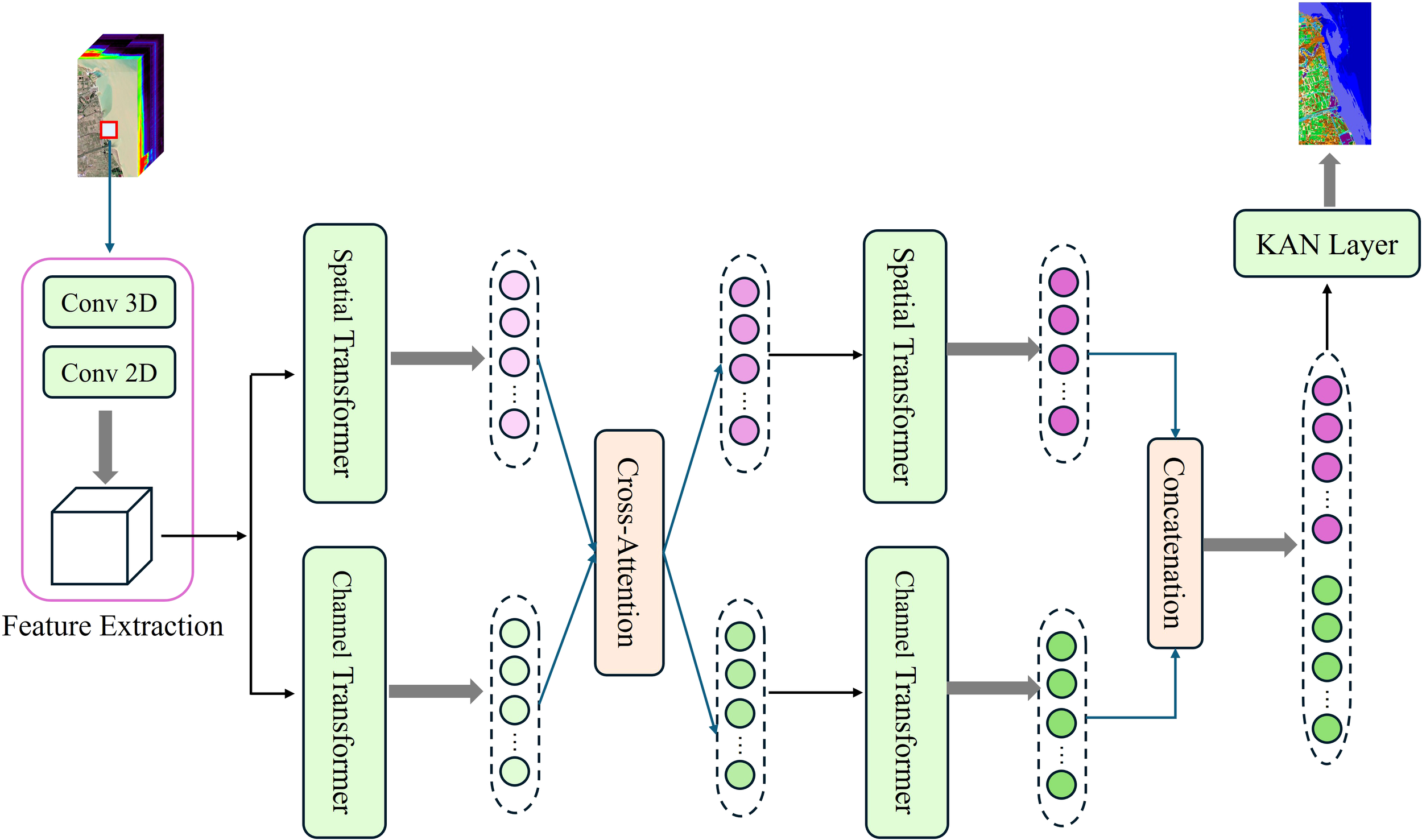
Schematic of the proposed algorithm framework. (1) Input hyperspectral patches undergo feature extraction to generate feature cubes. (2) The cubes are decomposed along spatial and channel dimensions for dual-branch Transformer processing. (3) Cross-attention modules enable feature interaction between branches. (4) Deep features are further extracted through additional dual-branch Transformer layers. (5) Final classification is achieved via KAN Layer after feature fusion.
2.1.1 Spatial-spectral feature extractor
Convolutional neural networks (CNNs) have demonstrated strong capabilities in hierarchical feature extraction. Wetland ecosystems exhibit complex spectral-spatial characteristics due to their diverse vegetation, water bodies, and transitional land cover. To effectively capture these features, we first employ a hybrid 3D-2D CNN feature extractor for preliminary spectral-spatial representation learning. The proposed feature extraction module integrates a sequential 3D convolutional block and a 2D convolutional block, each enhanced with Batch Normalization (BN) and nonlinear activation. The 3D convolution block primarily captures joint spectral and spatial information from each hyperspectral sample patch, while the 2D convolution block further refines spatial patterns from the output of the 3D convolution. This combination allows the model to effectively learn local spatial structures and retain spectral integrity. By leveraging the complementary strengths of both 3D and 2D convolutional operations, the proposed module fully exploits the multidimensional characteristics of hyperspectral imagery, providing a robust feature foundation for the subsequent classification task.
To prevent information loss at the image boundaries during patch extraction, zero-padding is applied to the hyperspectral images of coastal wetlands. The class label for each extracted patch is assigned based on the ground-truth label of its central pixel.
2.1.2 Dual-branch transformer encoder
Although the 3D-2D CNN feature extractor effectively captures low-level spectral-spatial patterns, wetland classification remains challenging due to the inherent spatial heterogeneity and subtle inter-class variations in coastal environments. To address these limitations and enhance the model’s ability to model complex spectral-spatial relationships and long-range dependencies, we introduce a dual-branch Transformer architecture based on feature cube decomposition. The feature cube generated based on the Feature Extraction structure, which defines its dimension as , is decomposed in this part along both spatial and channel directions. In the spatial direction, as shown in Figure 2a, the feature cube is decomposed into spatial tokens of size spatial tokens of size , where, represents the total number of spatial locations. This approach facilitates the modeling of inter-channel relationships, as each spatial token aggregates all channel information at a specific spatial location, enabling the capture of local features. In the channel direction, as illustrated in Figure 2b, the feature cube is decomposed into channel tokens . Each token focuses on a single channel and contains complete spatial information corresponding to that channel, helping preserve the spatial context.
Figure 2
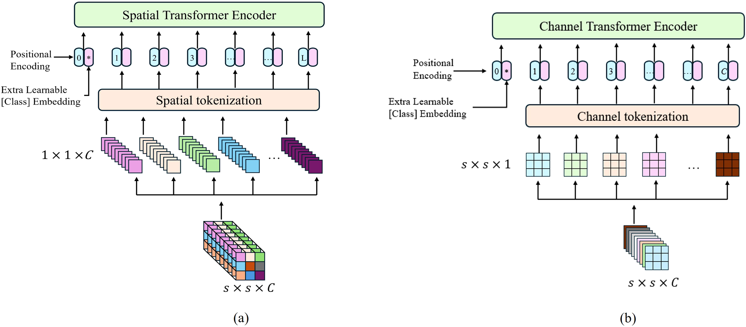
Schematic comparison of dual-branch Transformer architectures for hyperspectral feature decomposition. (a) Spatial transformer branch (b) Channel branch transformer.
For the spatial and channel branches, the input features are processed through a 3D convolutional kernel to generate feature chunks . As detailed in Equation 1, these chunks are then augmented with learnable category markers and position encoding parameters to construct the final marker sequence , which serves as the input to each Transformer encoder.
The main function of Transformer Encoder is feature extraction. It captures internal dependencies and high-level representations of the input data through multi-head attention mechanisms and feed-forward neural network.
2.1.3 Cross-attention mechanism
To enable dynamic feature interactions within our dual-branch Transformer architecture, we propose a cross-attention mechanism to facilitate adaptive feature enhancement between the two branches. This mechanism automatically identifies and amplifies the most discriminating features specific to different types of features in wetlands. Specifically, the cross-attention layer enables each element in one feature sequence to dynamically attend to and aggregate relevant information from the other sequence. This enhances feature correlations, provides richer contextual information, and improves the discriminative capability of the extracted features, thereby boosting classification accuracy. As illustrated in Figure 3, after feature transformation through the spatial and channel branches, cross-attention is applied to facilitate further interaction between the features extracted from the two branches. Specifically, one sequence is used to generate the query matrix, while the other provides the key and value matrices. The dot product between the query and all keys yields attention scores, which are normalized using the softmax function. The resulting weights are then used to compute a weighted sum of the values, forming the cross-attention output.
Figure 3
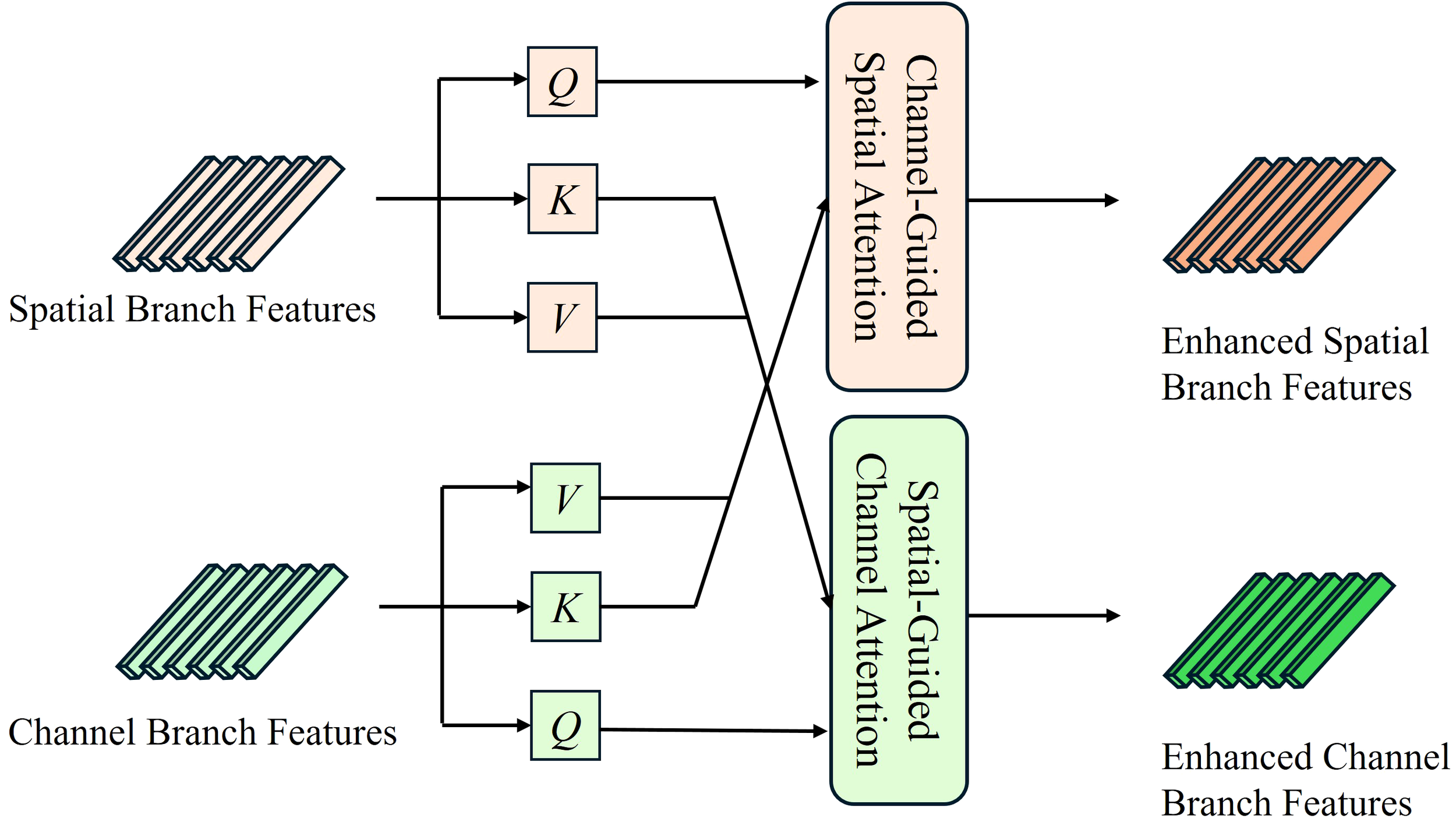
Schematic illustration of cross-attention between spatial and channel transformer branches: Dual-path feature interaction via bidirectional attention. CGSA (Channel-Guided Spatial Attention) enhances spatial features by querying channel branch KV, while SGCA (Spatial-Guided Channel Attention) refines channel features using spatial branch KV.
Specifically, prior to the cross-attention computation, this paper employs an asymmetric projection strategy to achieve spatial/channel feature space alignment. Spatial Transformer features Xspa are projected into Query , Key and Value , while the channel Transformer features Xcha are mapped to , Kcha .and respectively. The (Cross Attention Projection) operation asymmetrically maps dual-branch features to Query/Key/Value tensors as shown in Equation 2:
The cross-attention is then computed bidirectionally, as expressed in Equations 3 and 4:
Channel-Guided Spatial Attention(CGSA): leveraging channel information to enhance spatial representations.
Spatial-Guided Channel Attention(SGCA): utilizing spatial context to refine channel representations.
In the formulas (2) and (3), Queries () are always derived from the target branch, Keys/Values () come from features of the complementary branch, and denotes feature dimension of the Key.
Following the cross-attention operation, deeper feature extraction is required to better distinguish fine-grained intra-class characteristics. To this end, we introduce an additional dual-branch Transformer module following the cross-attention layer to further enhance high-level semantic representation learning. This module effectively captures the hyperspectral-spatial coupling characteristics of wetland data, thereby generating more discriminative representations for downstream classification. Finally, the complementary features from both branches are integrated through concatenation-based fusion.
2.1.4 Classification layer
The classification layer serves as the final mapping module to transform the extracted hierarchical features into categorical labels. Given the intricate nonlinear relationships inherent in coastal wetland ecosystems—interactions between different vegetation, soil types and hydrological conditions—we employ a Kolmogorov-Arnold Network (KAN) as a superior alternative to conventional multilayer perceptron (MLP) classifiers. The design of KAN is grounded in the Kolmogorov-Arnold representation theorem, allowing the network to process and learn complex relationships in input data in a way that approximates the theorem. Similar to MLP, KAN has a fully connected structure. However, unlike MLPs, which assign fixed activation functions to neurons (nodes), KAN assigns learnable activation functions to the edges (weights) of the network. This edge-based activation design provides greater flexibility in capturing nonlinear relationships within high-dimensional data, allowing the network to better fit intricate classification boundaries and improve performance in complex ecological classification tasks.
2.2 Datasets
In order to verify the effectiveness of the proposed method in coastal wetland hyperspectral image classification, two typical coastal wetland hyperspectral datasets were selected in this study —Yancheng wetland in Jiangsu Province and Yellow River Estuary wetland dataset.
2.2.1 Yancheng dataset
The Yancheng wetland is located in the eastern part of Jiangsu Province, China, and has a coastline of 582 kilometers, making it one of the largest coastal silt-flat wetlands on the west coast of the Pacific Ocean and on the edge of the Asian continent (Figure 4a). This wetland is highly valuable for ecological diversity, and it provides habitats for a variety of endangered species. In this study, the hyperspectral image dataset of coastal wetland in Yancheng, Jiangsu Province, acquired by the GF5_AHSI sensor, with an image size of 1175×585 and containing 253 effective spectral bands, was used. This dataset refers to the literature (Gao et al., 2022), and the spectral image processing team of Beijing Institute of Technology (BIT) deciphered the image by integrating the field survey data and the high spatial resolution images, and labeled the image with a total of 18 categories of feature classes, including salt fields, pond, paddy fields, woodland, buildings, etc. Table 1 presents the dataset partition, comprising 744 training samples and 7,150 testing samples, with the training set approximately accounting for 9.42% of the total samples, and 0.11% of the total pixels in the panoramic image.
Figure 4
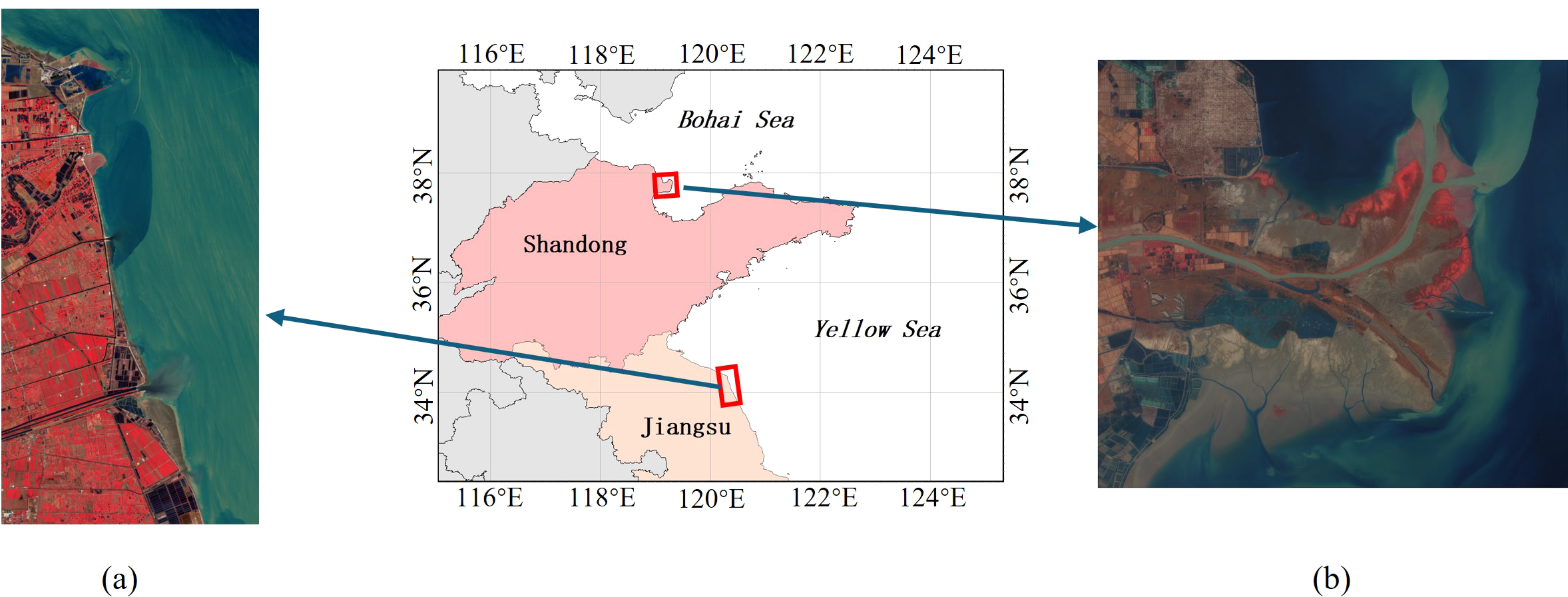
Location and false-color composite images of typical wetland datasets. (a) Yancheng wetland (b) Yellow River Estuary wetland.
Table 1
| The Yancheng dataset | The Yellow River Estuary dataset | ||||||
|---|---|---|---|---|---|---|---|
| No. | Name | Training | Testing | No. | Name | Training | Testing |
| 1 | Sea | 209 | 2186 | 1 | Spartina alterniflora | 162 | 15462 |
| 2 | Offshore area | 140 | 1448 | 2 | Pond | 98 | 6867 |
| 3 | Salt field | 6 | 104 | 3 | Woodland | 159 | 3298 |
| 4 | Pond | 20 | 173 | 4 | Phragmite | 75 | 7636 |
| 5 | Spartina anglica | 7 | 76 | 5 | Typha orientalis presl | 9 | 24 |
| 6 | Mudflats | 25 | 243 | 6 | Intertidal phragmite | 9 | 1407 |
| 7 | Aquaculture pond | 25 | 238 | 7 | Ecological reservoir | 50 | 3874 |
| 8 | Paddy field | 87 | 745 | 8 | Arable land | 98 | 10869 |
| 9 | Estuarine area | 27 | 248 | 9 | Lotus pond | 50 | 6448 |
| 10 | River | 27 | 272 | 10 | Oilfield | 162 | 7994 |
| 11 | Woodland | 19 | 196 | 11 | Salt fields | 75 | 8614 |
| 12 | Barren | 25 | 129 | 12 | Suaeda salsa | 147 | 10676 |
| 13 | Building | 37 | 489 | 13 | River | 49 | 1831 |
| 14 | Fallow land | 26 | 208 | 14 | Mixed area 1 | 25 | 1604 |
| 15 | Rainfed cropland | 28 | 176 | 15 | Mixed area 2 | 81 | 5455 |
| 16 | Suaeda salsa | 14 | 71 | 16 | Mixed area 3 | 9 | 128 |
| 17 | Irrigation canal | 10 | 28 | 17 | Mudflats | 81 | 5879 |
| 18 | Phragmites | 12 | 120 | 18 | Sea | 81 | 5463 |
| Total | 744 | 7150 | total | 1420 | 103529 | ||
Number of training and testing samples for coastal wetland datasets.
2.2.2 Yellow River Estuary dataset
The Yellow River Estuary wetland is located in the eastern part of the Yellow River Delta. It is rich in biological resources and provides habitat for many rare birds and plants (Figure 4b). In this study, the hyperspectral image data set of the Yellow River Estuary area was obtained by GF-5 AHSI sensor. The image size was 1185×1342, including 285 effective bands. Like the Yancheng wetland dataset, this dataset was also obtained from the spectral image processing team of Beijing Institute of Technology, and a total of 18 types of ground objects were marked, including spartina alterniflora, suaeda salsa, arable land, etc. Among them, Mixed area 1 is the mixed area of phragmites and tamarix, Mixed area 2 is the mixed area of tamarix and spartina alterniflora, and Mixed area 3 is the mixed area of tamarix, phragmites and spartina alterniflora. Table 1 summarizes the sample partitioning for model training and evaluation, with 1,420 samples allocated for training and 103,529 samples reserved for testing. The dataset samples represent 1.35% of the total samples and 0.089% of the panoramic pixels. This sparse training configuration intentionally challenges the model’s generalization capability under limited supervision.
3 Results
3.1 Experimental settings
In order to validate the effectiveness of the proposed method, we chose to conduct performance comparison experiments with several representative hyperspectral image classification related algorithms, including SVM (Melgani and Bruzzone, 2004), HE3DCNN (He, Li and Chen, 2017), HybridSN (Roy et al., 2020), SpectralFormer (Hong et al., 2022), SSFTT (Sun et al., 2022) and FactoFormer (Mohamed et al., 2024).
Specifically, this study employs the cross-entropy loss function (CrossEntropyLoss) as the optimization objective for the model, utilizing the Adam optimizer for parameter updates. To enhance the training process, we implement a stepwise learning rate decay strategy where the learning rate is multiplicatively reduced by a factor (set to 0.95 for both datasets in our experiments) after every training epochs. This scheduling strategy enables refined parameter adjustment during later training stages, thereby significantly improving convergence stability. For the Yancheng dataset, the patchsize is set to 5, with an initial learning rate of 9.8e-5 and a weight_decay of 9.9e-5. In contrast, for the Yellow River Estuary dataset, the patchsize is configured as 3, with both the initial learning rate and weight_decay set to 9.9e-5. For the SVM, we chose the radial Gaussian kernel function (RBF) for the classification task, and the penalty parameter and the kernel function parameter were determined by random search. HE3DCNN is a hyperspectral image classification model that combines 3D convolution and pyramid structure, the network settings refer to the literature, and the patchsize is set to 9 and 7 for Yancheng and Yellow River Estuary dataset respectively. HybridSN is a hybrid 2D and 3D convolutional approach, the dimensionality reduction procedure employes PCA with 15 principal components for both datasets, and the patchsize is 11, the learning rate of the optimizer is set to 0.001, and the value of weight_decay parameter is 1e-6. SpectralFormer is based on the Transformer architecture, which enhances the model’s ability to capture and represent spectral features through the perspective of serialization processing, in the Yancheng dataset, the patchsize is set to 5, and the bandpatch is set to 3, while in the Yellow River Estuary dataset, patchsize is set to 7, and bandpatch is set to 3. Other parameters are the same for both dataset, such as the mode is CAF, learning rate is set to 5e-4, and weight_decay is set to 5e-3. SSFTT is a hybrid structure of CNN and Transformer, for the Yancheng dataset, PCA is applied with 21 retained principal components, patchsize is set to 7, and the learning rate is set to 0.001, whereas in the Yellow River Estuary dataset, the number of PCA principal components is set to 15, and the patchsize is set to 11. In the FactoFormer method, for both datasets, the learning rate and the weight_decay are set to 1e-4, and the patchsize of Yancheng and Yellow River Estuary dataset are set to 5 and 3, respectively. In all the experiments, the epoch of each method is set to 200, and an early termination mechanism is adopted to prevent overfitting.
All experiments are conducted in a PyTorch environment running on a Windows 11 64-bit system with the following hardware configuration: an Intel Core i9-10900K Ultra 9 1850H processor (2.3GHz), 32GB RAM, 1TB SSD, and an NVIDIA RTX 3080 GPU (10GB VRAM). The computational environment utilizes CUDA 12.4 and cuDNN 9.0 for accelerated processing.
In order to quantitatively analyze the effectiveness of the proposed method and other comparative methods, four quantitative assessment metrics were introduced, including overall accuracy (OA), average accuracy (AA), kappa coefficient (κ), and classification accuracy for each land cover category. A larger value for each indicator indicates a better classification effect.
3.2 Quantitative analysis
Through comprehensive comparison with representative hyperspectral image classification approaches (Tables 2, 3), our method demonstrates competitive performance on both coastal wetland datasets (Yancheng and Yellow River Estuary). The tabulated results highlight our method’s superiority, with optimal and sub-optimal metrics indicated in bold and underlined text, respectively.
Table 2
| Class | SVM | HE3DCNN | HybridSN | SpectralFormer | SSFTT | FactoFormer | Proposed method |
|---|---|---|---|---|---|---|---|
| 1 | 81.71 | 92.91 | 92.50 | 99.13 | 94.74 | 100.00 | 98.12 |
| 2 | 100.00 | 98.90 | 99.93 | 100.00 | 99.31 | 100.00 | 100.00 |
| 3 | 58.65 | 25.00 | 56.73 | 69.23 | 64.42 | 48.08 | 54.81 |
| 4 | 87.86 | 71.68 | 77.46 | 80.35 | 80.92 | 80.35 | 79.19 |
| 5 | 100.00 | 82.89 | 100.00 | 86.84 | 90.79 | 94.74 | 100.00 |
| 6 | 83.13 | 77.78 | 87.65 | 78.60 | 94.24 | 87.65 | 95.47 |
| 7 | 75.63 | 82.77 | 89.50 | 90.76 | 92.02 | 77.31 | 92.02 |
| 8 | 97.32 | 95.44 | 99.46 | 96.38 | 97.18 | 98.26 | 99.73 |
| 9 | 98.39 | 84.68 | 94.35 | 98.79 | 95.56 | 93.55 | 98.39 |
| 10 | 81.25 | 95.96 | 58.09 | 94.12 | 71.69 | 95.59 | 97.79 |
| 11 | 97.96 | 84.69 | 100.00 | 100.00 | 100.00 | 100.00 | 100.00 |
| 12 | 100.00 | 62.79 | 96.90 | 94.57 | 98.45 | 98.45 | 98.45 |
| 13 | 80.37 | 85.48 | 93.46 | 83.03 | 99.18 | 86.91 | 97.14 |
| 14 | 95.67 | 85.10 | 82.69 | 87.98 | 95.19 | 92.31 | 91.35 |
| 15 | 93.75 | 95.45 | 68.18 | 78.98 | 98.30 | 96.02 | 97.16 |
| 16 | 80.28 | 66.20 | 88.73 | 84.51 | 95.77 | 67.61 | 76.06 |
| 17 | 78.57 | 100.00 | 57.14 | 100.00 | 82.14 | 64.29 | 96.43 |
| 18 | 68.33 | 59.17 | 57.50 | 58.33 | 65.83 | 80.83 | 78.33 |
| OA(%) | 88.59 | 89.51 | 91.12 | 94.01 | 94.24 | 94.94 | 96.52 |
| AA(%) | 86.60 | 80.38 | 83.35 | 87.87 | 89.76 | 86.77 | 91.69 |
| κ | 0.8668 | 0.8761 | 0.8951 | 0.9289 | 0.9319 | 0.9398 | 0.9587 |
Class-specific classification accuracy (%) using different methods on the Yancheng dataset (bold and underlined values indicate optimal and suboptimal indicators respectively).
Table 3
| Class | SVM | HE3DCNN | HybridSN | SpectralFormer | SSFTT | FactoFormer | Proposed method |
|---|---|---|---|---|---|---|---|
| 1 | 91.19 | 91.55 | 96.98 | 85.75 | 79.39 | 95.87 | 91.73 |
| 2 | 87.81 | 69.74 | 92.46 | 78.72 | 99.33 | 71.33 | 81.93 |
| 3 | 95.45 | 97.18 | 86.45 | 92.78 | 67.62 | 94.21 | 97.73 |
| 4 | 66.41 | 77.85 | 83.16 | 53.41 | 77.30 | 74.16 | 62.70 |
| 5 | 100.00 | 100.00 | 100.00 | 100.00 | 100.00 | 100.00 | 100.00 |
| 6 | 77.19 | 46.34 | 76.83 | 90.62 | 92.25 | 87.42 | 84.65 |
| 7 | 89.18 | 89.21 | 89.24 | 79.84 | 84.23 | 92.20 | 94.48 |
| 8 | 74.02 | 89.82 | 90.46 | 88.62 | 78.35 | 89.61 | 98.64 |
| 9 | 71.25 | 71.68 | 70.46 | 72.83 | 74.12 | 77.08 | 80.29 |
| 10 | 88.10 | 98.86 | 91.53 | 49.04 | 94.43 | 88.49 | 89.93 |
| 11 | 68.12 | 45.15 | 48.68 | 66.95 | 64.60 | 82.34 | 70.10 |
| 12 | 85.84 | 95.06 | 86.95 | 90.12 | 94.26 | 84.92 | 95.04 |
| 13 | 100.00 | 99.13 | 100.00 | 100.00 | 98.36 | 100.00 | 100.00 |
| 14 | 51.12 | 16.96 | 30.11 | 49.94 | 43.33 | 44.26 | 50.94 |
| 15 | 70.03 | 95.29 | 90.89 | 72.81 | 85.26 | 79.60 | 83.83 |
| 16 | 92.19 | 25.00 | 91.41 | 99.22 | 100.00 | 84.38 | 100.00 |
| 17 | 67.89 | 67.89 | 66.75 | 67.89 | 64.65 | 67.89 | 67.89 |
| 18 | 61.08 | 95.31 | 89.99 | 96.01 | 97.79 | 100.00 | 99.60 |
| OA(%) | 78.77 | 82.17 | 83.56 | 77.08 | 81.82 | 84.72 | 85.72 |
| AA(%) | 79.83 | 76.22 | 82.35 | 79.70 | 83.07 | 84.10 | 86.08 |
| κ | 0.7695 | 0.8059 | 0.8212 | 0.7513 | 0.8026 | 83.38 | 0.8446 |
Class-specific classification accuracy (%) using different methods on the Yellow River Estuary dataset (bold and underlined values indicate optimal and suboptimal indicators respectively).
3.2.1 Yancheng dataset
Table 2 shows the performance comparison results of each classification algorithm on Yancheng dataset. Experimental results reveal that the conventional SVM approach, relying exclusively on basic spectral feature processing, demonstrates classification deficiencies. The method underperforms notably for water-related categories, including sea (Class 1), aquaculture pond (Class 7), and irrigation canal (Class 17), achieving an OA value of 88.59%. HE3DCNN employs 3D convolution for spectral-spatial feature extraction and incorporates a pyramid structure for multi-scale feature fusion, achieving an overall accuracy (OA) of 89.51% on the Yancheng dataset. HybridSN method achieves a detailed joint spatial-spectral feature extraction process due to combining the structural features of 2DCNN and 3DCNN and obtains 91.12% OA value, but performs poorly on river, fallow land, rainfed cropland, etc (Class 10/14/15/17/18). SpectralFormer learns spectrally localized sequence information from neighboring bands of hyperspectral images and designs cross-layer jump connections to significantly improve the robustness of feature representation, which achieves OA of 94.01% and AA of 87.87% for the classification task on the Yancheng dataset, but performs poorly on categories such as mudflats (Class 6) and phragmites (Class 18). The SSFTT achieves joint extraction of spatial and spectral features by combining the advantages of CNN and Transformer, showing competitiveness in OA, AA and KAPPA, but poor performance in the river category (Class 10). The FactoFormer method employs a dual-branch spatial and spectral channel modeling process and introduces self-supervised pre-training mechanism, attains 94.94% OA on Yancheng dataset, though performance degrades for aquaculture ponds (Class 7) and irrigation channels (Class 17). The proposed method in this study integrates the advantages of CNN and Transformer, and adopts the dual-branch spatial and channel modeling design to ensure more comprehensive information acquisition. Cross-attention further realizes the fusion of different forms of features and a more detailed feature extraction process, which enables the proposed method to have a better classification performance on the Yancheng dataset, and outperforms other comparative methods in terms of OA, AA, and Kappa.
3.2.2 Yellow River Estuary dataset
Table 3 demonstrates the performance comparison results of each classification algorithm on the Yellow River Estuary dataset. The distinctive feature of this dataset is that the vegetation mixing region of tamarisk, phragmites and spartina alterniflora is considered (class 14/15/16), and the proportion of training samples in the whole region is exceptionally limited. As can be seen from the results, the performances of all the classification methods on this dataset decreased, with the OA values dropping to the range of 77.08% to 85.72%. The SVM method is accurate for the classification of typha orientalis presl (class 5) and river (class 13), and so are the other methods in the paper, but performs moderately well in the recognition of most of the features. The HE3DCNN method is the most effective for the extraction of the oil field (class 10), but the recognition efficacy for the mixed zone is significantly decreased, especially for mixed area 2 (class 14) and 3 (class 16). The HybridSN method excelled in the extraction of spartina alterniflora (class 1) and mixed area 2 (class 15), but performs poorly in the identification of areas of phragmites and tamarisk mixing. The SpectralFormer method performs well for intertidal phragmite (class 6) and for mixing areas 3 (class 16), but performs poorly on aquaculture pond (class 7), river (class 10), and mixed area 2 (class 15) categories. The SSFTT method performs best in pond (class 2), intertidal phragmites (class 6), and oil field (class 10) extraction and is accurate for the identification of the mixed area 3(class 16). FactoFormer is accurate for the identification of sea(class 18), and has the best performance for the salt field (class 11), which is superior to the other methods, but does not perform well for the mixed area 3. The proposed method demonstrated overall superior classification performance on the Yellow River Estuary dataset, with overall accuracy (OA=85.72%) and average accuracy (AA=86.08%) significantly better than all the comparative methods, and the Kappa coefficient (0.8446) reached the reliability level of “almost perfect agreement”. The method accurately recognizes three categories (class 5/13/16), performs best in five other categories (class 3/7/8/9/17), and achieves secondary-best performance in four categories (class 11/12/14/18). Overall, for the Yellow River Estuary dataset, this paper’s method outperforms other comparative methods in categorization and excels in mixed zone extraction.
3.3 Qualitative analysis
To visually evaluate the performance of different classification methods in coastal wetland scenarios, this part generates complete fully labeled classification maps for the 2 datasets of Yancheng and Yellow River Estuary respectively, as shown in Figures 5, 6.
Figure 5
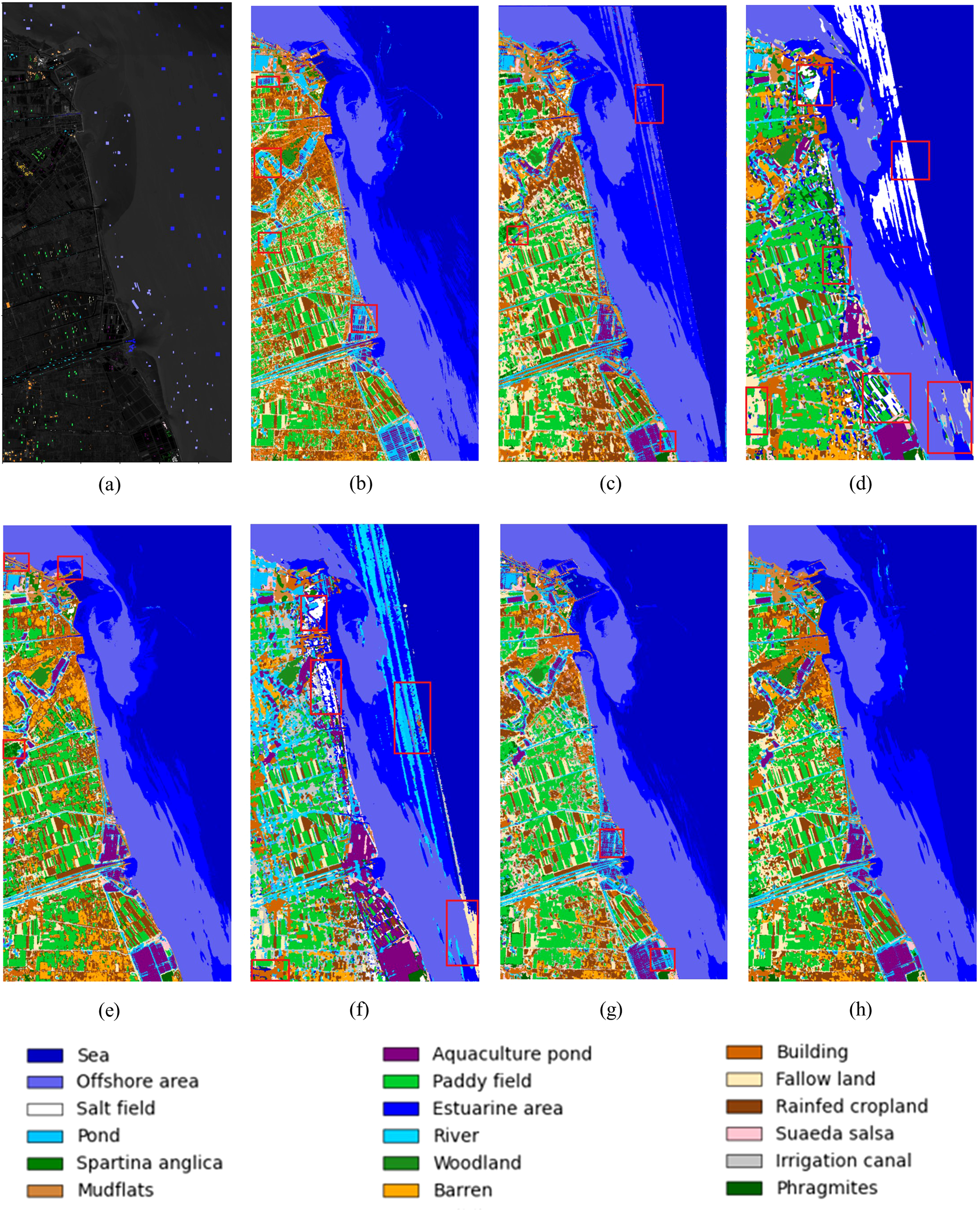
Full classification maps obtained by different models on the Yancheng dataset. (a)groundtruth (b) SVM (c) HE3DCNN (d) HyBridSN (e) SpectralFormer (f) SSFTT (g) FactoFormer (h) proposed method.
Figure 6
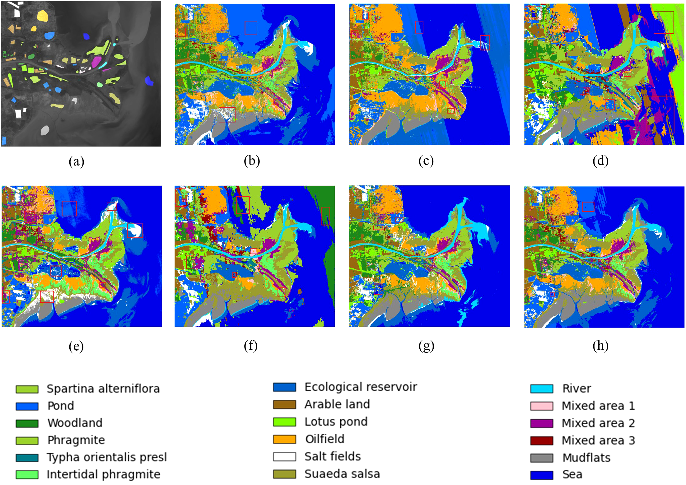
Full classification maps obtained by different models on the Yellow River Estuary dataset (a) groundtruth (b)SVM (c) HE3DCNN (d) HyBridSN (e) SpectralFormer (f) SSFTT (g) FactoFormer (h) proposed method.
3.3.1 Yancheng dataset
From the wetland fully labeled classification map, it can be seen that most classification methods have significant attenuation of accuracy in specific feature types, constrained by the heterogeneity of complex wetland ecosystems and the separability between feature classes. For the Yancheng dataset, the SVM method is ineffective on aquaculture pond (class 7) and irrigation canals (class 17), and it is easy to misclassify aquaculture pond as pond and misclassify irrigation canals as fallow land. Similarly, the HE3DCNN method has significant streaking noise on the sea surface and misclassify the aquaculture pond as phragmites. The HyBridSN method has more severe streaking on the sea surface, and performs poorly in the extraction of river (class 10), fallow land (class 14), rainfed cropland (class 15), irrigation canal (class 17) extraction, misclassifying rainfed cropland as salt field, or due to the similarity in SWIR reflectance properties of salt field crystals and arid rainfed cropland. The SpectralFormer method misclassified features the extraction of spartina anglica (class 5), mudflats (class 6), buildings (class 13), rainfed cropland (class 15), etc. The SSFTT has severe streaking on the sea surface, and the accuracy of rivers (class 10) and phragmites (class 18) is poor, and misclassified near-shore vegetation into salt field or sea water due to the influence of seawater impregnation of the intertidal vegetation. FactoFormer performs poorly for aquaculture ponds (class 7) and irrigation canals (class 17), and is prone to misclassify aquaculture ponds (class 7) as ponds or rivers. In most of the misclassified categories (class 7/10/15/17/18), the proposed method performs stably and shows obvious advantages in the stability of classification of typical wetland features.
3.3.2 Yellow River Estuary dataset
For the Yellow River Estuary dataset, the SVM method misclassifies arable land (class 8) as oilfield, Mixed area 2 (class 15) as other categories, suaeda salsa as salt fields, and the offshore north of the Yellow River Estuary (class 18) as other water bodies such as pond. HE3DCNN in the sea surface (class 18) has regular streak noise, misclassifies intertidal phragmite (class 6) as oilfield or suaeda salsa, misclassifies salt fields (class 11) into pond or ecological reservoir, and performs poorly in mixed vegetation area (class 15/16). The HyBridSN method demonstrates strong classification accuracy for spartina alterniflora (class 1), typha orientalis presl (class 5), and river (class 13). However, it shows notable misclassification issues in other categories, including weak Sea detection and frequent confusion between intertidal Phragmites (class 6) and suaeda salsa (class12). The SpectralFormer method misclassifies suaeda salsa as Salt Fields, ecological reservoir (class 7) as pond or sea, and confused oilfield (class 10) with mixed area 2 (Class 15). Additionally, it erroneously labels the boundary between river and sea as salt fields. The SSFTT method shows significant large-scale misclassification in the sea area, and woodland (class 3) is misidentified as the tamarix- spartina alterniflora mixed growing area. Arable land (class 8) exists confusion with pond, lotus pond and other water bodies, mixed area 1 (class 14) is misidentified as phragmite community. The self-supervised pre-training mechanism of FactoFormer effectively suppresses the misclassification of sea, but at the same time, there are some limitations, misclassifying wetland water bodies as ocean types, misclassifying pond (class 2) as salt fields, and extracting poorly for the mixed region of tamarisk-phragmite-spartina alterniflora (class 16, mixed area 3).The research method in this paper shows confusing classification with ponds in the offshore area north of the Yellow River Estuary. Systematic comparative experiments demonstrate that this misclassification prevails across multiple benchmark methods (SVM, HE3DCNN, HyBridSN, SpectralFormer, and SSFTT). We attribute this phenomenon to: (1) spatial adjacency between coastal waters and pond complexes, and (2) hydrological connectivity (e.g., tidal channels) inducing feature homogenization in spectral-spatial domains. Overall, our method exhibits superior robustness to other methods for the easily confounded categories (class8/11) and mixed vegetation areas (class14/15/16).
4 Discussion
To comprehensively evaluate the contribution of each module in the proposed method, we conducted systematic ablation studies on both the Yancheng and Yellow River Estuary datasets by examining different component combinations. The proposed framework consists of five key components: Feature Extractor (FE), Dual-Branch Transformer1 (DBT1), Cross Attention (CA), Dual-Branch Transformer2 (DBT2), and KAN modules. Through incremental removal of each module, we analyzed their individual and collective effects on model performance across the two datasets. Specifically, Table 4 presents the overall performance comparison of the Yancheng dataset under different ablation cases, while Table 5 details the classification accuracy of each feature category across these cases. The Yellow River Estuary dataset follows the same ablation approach, with its detailed classification results summarized in Table 6. Figures 7, 8 present the panoramic prediction results of the Yancheng and Yellow River Estuary datasets under different ablation study cases, respectively.
Table 4
| Cases | Components | Indicators | ||||||
|---|---|---|---|---|---|---|---|---|
| FE | DBT1 | CA | DBT2 | KAN | OA(%) | AA(%) | κ | |
| 1 | × | ✓ | ✓ | ✓ | ✓ | 63.47 | 31.63 | 0.5577 |
| 2 | ✓ | × | ✓ | ✓ | ✓ | 95.68 | 86.31 | 0.9486 |
| 3 | ✓ | ✓ | × | × | ✓ | 95.30 | 88.69 | 0.9444 |
| 4 | ✓ | ✓ | × | ✓ | ✓ | 96.06 | 87.45 | 0.9531 |
| 5 | ✓ | ✓ | ✓ | × | ✓ | 93.80 | 86.01 | 0.9268 |
| 6 | ✓ | ✓ | ✓ | ✓ | MLP | 91.69 | 88.13 | 0.9026 |
| 7 | ✓ | ✓ | ✓ | ✓ | ✓ | 96.52 | 91.69 | 0.9587 |
Ablation study configurations (✓: present; ×: absent) on Yancheng dataset (optimal results are bolded).
Table 5
| Class | Case 1 | Case 2 | Case 3 | Case 4 | Case 5 | Case 6 | Proposed method |
|---|---|---|---|---|---|---|---|
| 1 | 100.00 | 98.99 | 95.56 | 99.27 | 93.55 | 86.18 | 98.12 |
| 2 | 100.00 | 100.00 | 100.00 | 100.00 | 100.00 | 99.93 | 100.00 |
| 3 | 56.73 | 23.08 | 38.46 | 29.81 | 33.65 | 55.77 | 54.81 |
| 4 | 0.00 | 84.98 | 80.92 | 83.24 | 80.35 | 75.14 | 79.19 |
| 5 | 2.63 | 30.26 | 50.00 | 34.21 | 26.32 | 56.58 | 100.00 |
| 6 | 95.47 | 95.06 | 94.65 | 91.36 | 95.88 | 90.53 | 95.47 |
| 7 | 0.42 | 88.24 | 91.18 | 89.08 | 89.08 | 89.50 | 92.02 |
| 8 | 13.15 | 99.87 | 99.73 | 99.06 | 98.79 | 97.99 | 99.73 |
| 9 | 4.03 | 98.79 | 98.79 | 100.00 | 100.00 | 98.79 | 98.39 |
| 10 | 72.43 | 97.79 | 99.26 | 98.90 | 98.16 | 96.32 | 97.79 |
| 11 | 2.55 | 100.00 | 100.00 | 100.00 | 100.00 | 100.00 | 100.00 |
| 12 | 45.74 | 100.00 | 99.22 | 100.00 | 99.22 | 100.00 | 98.45 |
| 13 | 46.01 | 97.75 | 98.16 | 98.77 | 92.64 | 91.82 | 97.14 |
| 14 | 0.00 | 95.67 | 97.60 | 98.56 | 99.04 | 98.56 | 91.35 |
| 15 | 5.11 | 96.02 | 95.45 | 96.59 | 97.16 | 94.89 | 97.16 |
| 16 | 0.00 | 74.65 | 77.46 | 76.06 | 70.42 | 71.83 | 76.06 |
| 17 | 0.25 | 100.00 | 100.00 | 100.00 | 96.43 | 100.00 | 96.43 |
| 18 | 0.00 | 72.50 | 80.00 | 79.17 | 77.50 | 82.50 | 78.33 |
| OA(%) | 63.47 | 95.68 | 95.30 | 96.06 | 93.80 | 91.69 | 96.52 |
| AA(%) | 31.63 | 86.31 | 88.69 | 87.45 | 86.01 | 88.13 | 91.69 |
| κ | 0.5577 | 0.9486 | 0.9444 | 0.9531 | 0.9248 | 0.9026 | 0.9587 |
Detailed categorization results of ablation experiments on the Yancheng dataset (optimal results are bolded).
Table 6
| Class | Case 1 | Case 2 | Case 3 | Case 4 | Case 5 | Case 6 | Proposed method |
|---|---|---|---|---|---|---|---|
| 1 | 2.92 | 93.47 | 93.82 | 93.02 | 92.82 | 90.23 | 91.73 |
| 2 | 88.93 | 82.00 | 85.38 | 81.17 | 84.14 | 81.93 | 81.93 |
| 3 | 13.10 | 99.70 | 99.30 | 99.82 | 97.79 | 97.30 | 97.73 |
| 4 | 15.57 | 67.26 | 66.13 | 70.99 | 49.70 | 73.11 | 62.70 |
| 5 | 0.00 | 100.00 | 100.00 | 100.00 | 100.00 | 100.00 | 100.00 |
| 6 | 0.07 | 87.92 | 80.38 | 84.51 | 73.13 | 69.94 | 84.65 |
| 7 | 0.09 | 96.54 | 96.62 | 95.95 | 95.51 | 88.05 | 94.48 |
| 8 | 76.95 | 97.12 | 97.09 | 92.10 | 98.63 | 98.74 | 98.64 |
| 9 | 3.74 | 73.98 | 72.15 | 75.96 | 69.26 | 80.97 | 80.29 |
| 10 | 66.88 | 91.52 | 90.23 | 92.98 | 90.41 | 81.44 | 89.93 |
| 11 | 0.30 | 69.93 | 73.08 | 72.83 | 77.15 | 56.52 | 70.10 |
| 12 | 0.00 | 93.25 | 96.62 | 94.99 | 98.00 | 95.63 | 95.04 |
| 13 | 100.00 | 100.00 | 100.00 | 100.00 | 100.00 | 100.00 | 100.00 |
| 14 | 3.62 | 48.13 | 62.22 | 46.76 | 52.49 | 57.86 | 50.94 |
| 15 | 20.13 | 77.76 | 64.82 | 75.51 | 74.35 | 71.11 | 83.83 |
| 16 | 37.50 | 100.00 | 49.22 | 92.19 | 100.00 | 47.66 | 100.00 |
| 17 | 13.64 | 67.89 | 67.31 | 67.43 | 37.32 | 67.55 | 67.89 |
| 18 | 95.73 | 100.00 | 100.00 | 100.00 | 100.00 | 100.00 | 99.60 |
| OA(%) | 30.51 | 85.54 | 85.45 | 85.58 | 84.71 | 83.51 | 85.72 |
| AA(%) | 30.47 | 85.91 | 83.02 | 85.34 | 84.48 | 81.00 | 86.08 |
| κ | 0.2543 | 0.8427 | 0.8416 | 0.8431 | 0.8335 | 0.8205 | 0.8446 |
Detailed categorization results of ablation experiments on the Yellow River Estuary dataset (optimal results are bolded).
Figure 7
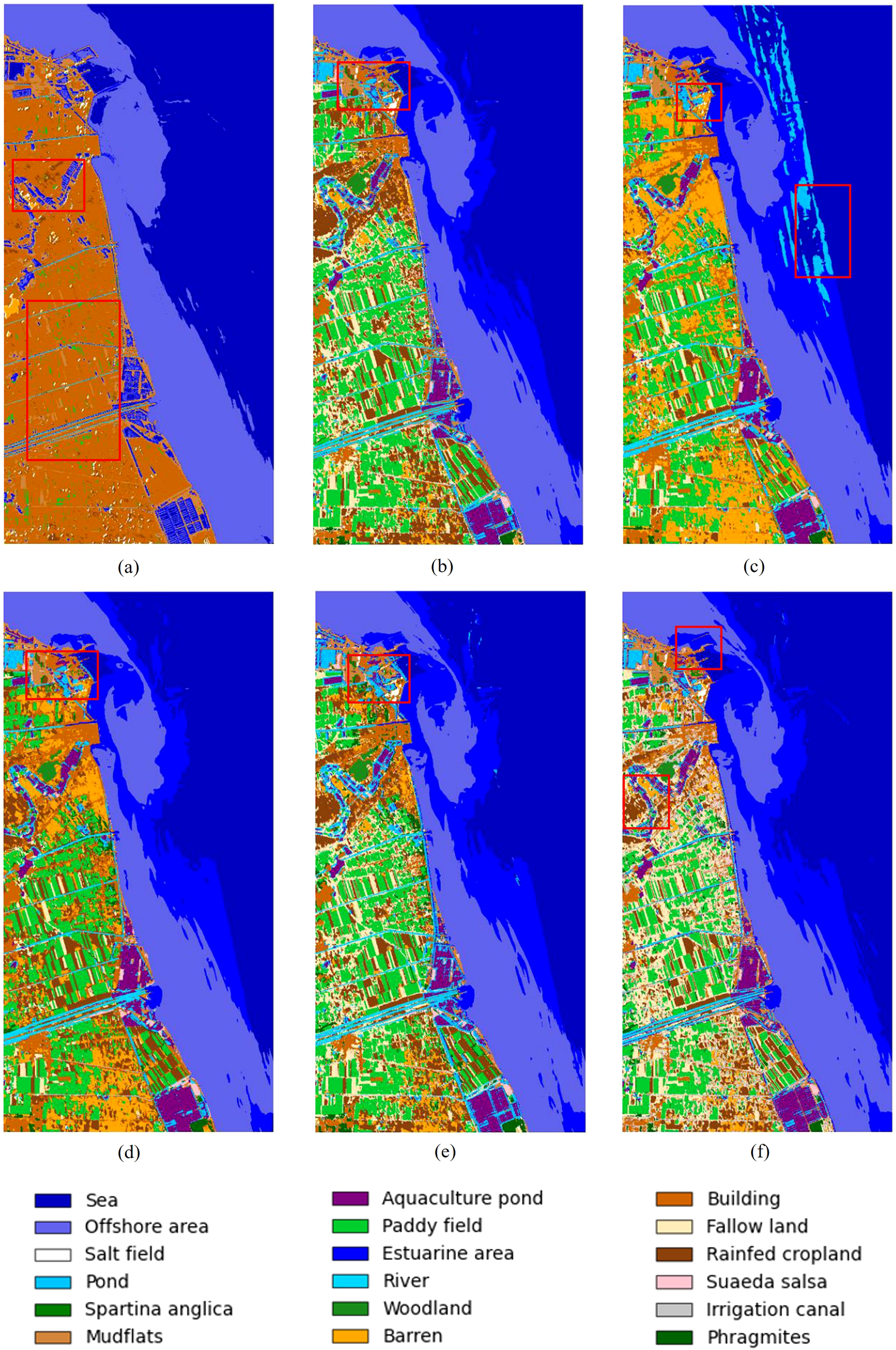
Full classification maps of the Yancheng dataset under different ablation study cases. (a) our model without FE module (b) without DBT1 module (c) without CA and DBT2 module (d) without CA module (e) without DBT2 module (f) with MLP as the classification head.
Figure 8
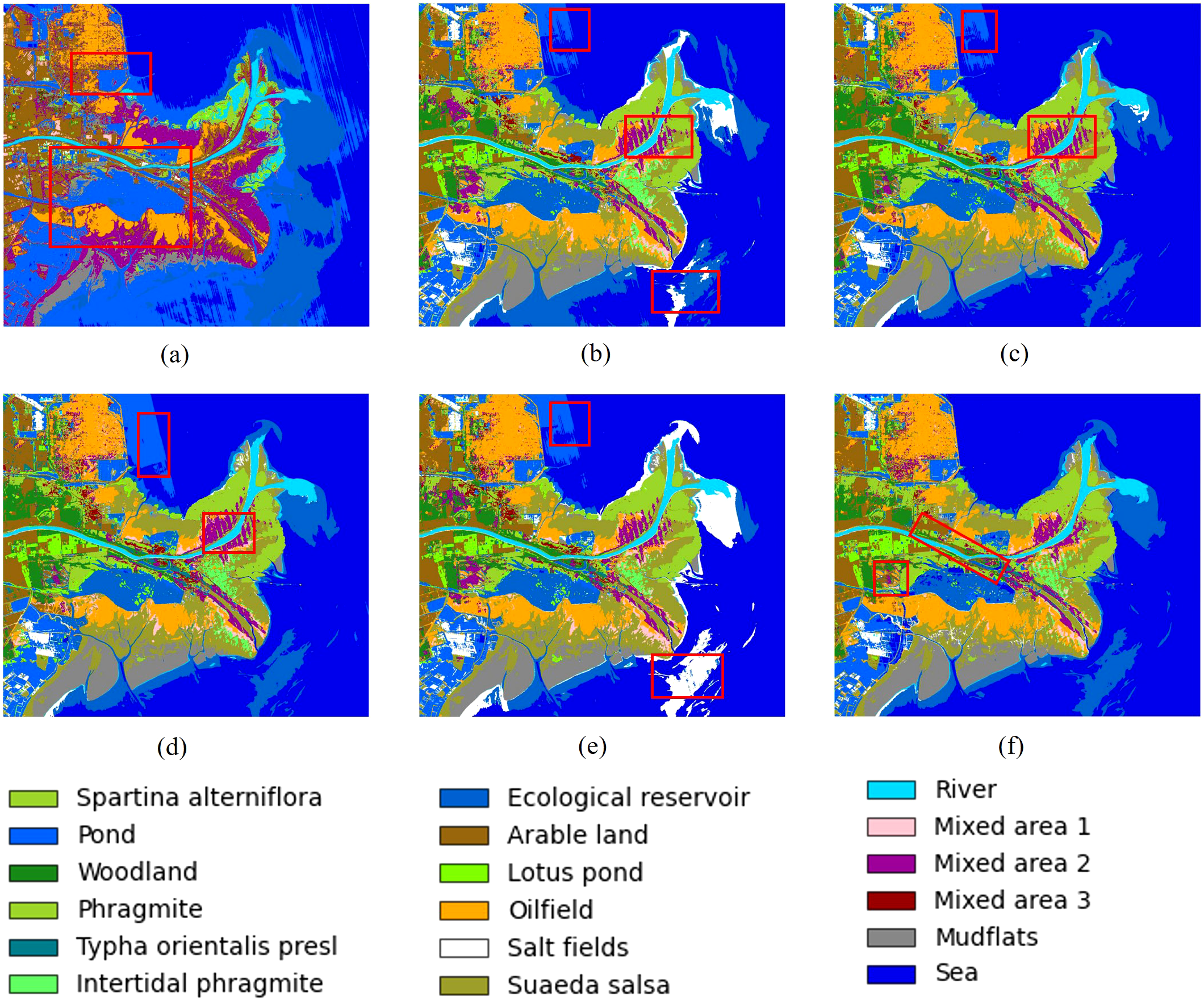
Full classification maps of the Yellow River Estuary dataset under different ablation study cases. (a) our model without FE module (b) without DBT1 module (c) without CA and DBT2 module (d) without CA module (e) without DBT2 module (f) with MLP as the classification head.
The ablation study results demonstrate that each component of the proposed model contributes significantly to the final wetland classification performance. Specifically:
The FE module effectively captures joint spatial-spectral features of the wetland hyperspectral data through its 3D CNN architecture, while the subsequent 2D CNN further enhances spatial feature abstraction. This design proves particularly effective for characterizing environments with high spatial heterogeneity. When the FE module is removed (Case 1), the model experiences a substantial performance degradation, with OA dropping to 63.47% for the Yancheng dataset and merely 30.51% for the Yellow River Estuary dataset. These results not only confirm the module’s critical role in wetland feature extraction but also underscore its particular importance in scenarios characterized by high environmental heterogeneity.
When the DBT1 module is ablated (Case 2), the overall classification accuracy remains high. However, performance deteriorates significantly for certain fine-grained categories. Specifically, the model exhibits notable deficiencies in Salt field and Spartina anglica in the Yancheng dataset, as well as the mixed vegetation community of tamarix and spartina alterniflora (Mixed Area 2) in the Yellow River Estuary dataset. This observation suggests that the DBT1 module plays a critical role in enhancing the model’s ability to discriminate subtle inter-class variations, particularly in mixed wetland vegetation. By leveraging parallel spatial and channel long-range dependency modeling, DBT1 provides more discriminative feature representations for downstream processing.
The CA module improves the model’s discriminative capacity for subtle variations by effectively integrating spatial and channel-wise interaction features. Ablation of the CA module (Case 3) leads to performance degradation in several key categories: classification accuracy decreases for Sea, Salt field and Spartina anglica in the Yancheng dataset, accompanied by pronounced streak anomaly on sea surface classification. Similarly, the model exhibits significantly reduced accuracy for Mixed Area 2 and 3 in the Yellow River Estuary dataset compared to the full model. These results demonstrate that the CA module plays a crucial role in enhancing feature discrimination, particularly for challenging cases involving fuzzy boundaries and mixed vegetation communities, through feature interaction capability.
The DBT2 module serves as a secondary refinement unit to enhance classification stability in complex land cover scenarios. Ablation studies (Case 5) reveal that the full model (Case 7) achieves consistent improvements in OA, AA, and KAPPA metrics across both datasets, demonstrating the necessity of deep feature extraction following cross-attention. Comparative analysis between Cases 4 and 3 shows that DBT2 improves classification accuracy for Sea in the Yancheng dataset while eliminating sea surface streak anomaly. Similarly, in the Yellow River Estuary dataset, DBT2 enhances classification performance for mixed vegetation communities (Mixed Area 2 and 3). These results indicate that DBT2’s dual-branch Transformer architecture, through its secondary refinement of spatial and channel features, improves the model’s discriminative capacity for different water bodies and mixed vegetation environments.
Compared to using MLP as the classification head (Case 6), the KAN module (Case 7) strengthens model discriminability through nonlinear feature mapping, improving overall classification accuracy across both datasets. The KAN module’s adaptive nonlinear learning capability enables more effective modeling of dynamic wetland cover variations, demonstrating strong compatibility with the heterogeneous nature of wetland environments.
The ablation studies comprehensively validate the efficacy and synergistic integration of the proposed modular architecture: (1) The FE module establishes fundamental feature representations to address environmental heterogeneity; (2) The DBT1 module refines feature expression to capture inter-class variations; (3) The CA module enhances feature interactions for improved characterization of complex vegetation communities; (4) The DBT2 module enables deeper feature abstraction, particularly for discriminating distinct water bodies and mixed vegetation features; and (5) The KAN module’s nonlinear classification head adapts to fuzzy boundaries and dynamic surface cover changes. Collectively, this hierarchical framework provides an effective solution for wetland hyperspectral image classification, by synergistically integrating hierarchical feature extraction with multidimensional feature interaction.
5 Conclusion
In this paper, we propose a hyperspectral image classification method tailored for coastal wetlands. The method integrates the advantages of convolutional neural network (CNNs) and Transformer architectures, and progressively extracts low, middle, and high level features sequentially through hierarchical framework. Specifically, 3D and 2D convolutional layers are employed to fully capture low-level spectral and spatial features, while the combination of dual-branch Transformers with a cross-attention mechanism enable multi-dimensional feature fusion and the extraction of high-level semantic representations. Experiment results demonstrate that the proposed method significantly enhances classification performance on hyperspectral images of coastal wetlands, particularly for typical land cover types such as mudflats and mixed vegetation areas. In future work, strategies to improve model performance under small-sample conditions will be explored. These may include the application of semi-supervised learning, self-supervised learning, and domain adaptation techniques to effectively utilize both limited labeled samples and large volumes of unlabeled data, thereby enhancing the generalization ability of the model.
Statements
Data availability statement
Publicly available datasets were analyzed in this study. This data can be found here: The data analyzed in this study was obtained from the 2024 Chinese Workshop on Hyperspectral Earth Observation (https://hsi.ecnu.edu.cn), processed by the spectral image processing team of Beijing Institute of Technology. Requests to access these datasets should be directed to the workshop organizing committee at committee@ce.ecnu.edu.cn.
Author contributions
ZL: Formal Analysis, Methodology, Software, Validation, Visualization, Writing – original draft. TL: Conceptualization, Methodology, Writing – review & editing, Funding acquisition. YL: Methodology, Software, Writing – review & editing. JT: Conceptualization, Writing – review & editing. MZ: Writing – review & editing, Conceptualization, Supervision. CZ: Conceptualization, Writing – review & editing, Project administration, Resources.
Funding
The author(s) declare that financial support was received for the research and/or publication of this article. This study is financially supported by the International Partnership Program by the Chinese Academy of Sciences under Grant 121311KYSB20190029.
Acknowledgments
The authors extend sincere gratitude to Dr. Wanli Zhang for his expert guidance in methodological discussions and generous provision of high-performance computing resources. The coastal wetland hyperspectral datasets employed are obtained from the 2024 China Hyperspectral Earth Observation Symposium, meticulously preprocessed by the Spectral Image Processing Team at Beijing Institute of Technology. We extend our sincere gratitude to the laboratory for their open-access provision of these mission-critical datasets. Finally, the code implementation draws upon methodologies from SpectralFormer and FactoFormer, gratefully acknowledge Danfeng Hong, Mohamed et al. for making their open-source codebase publicly available.
Conflict of interest
The authors declare that the research was conducted in the absence of any commercial or financial relationships that could be construed as a potential conflict of interest.
The reviewer CX declared a shared affiliation with the authors ZL, TL, YL, CZ to the handling editor at the time of review.
Generative AI statement
The author(s) declare that Generative AI was used in the creation of this manuscript. For linguistic enhancement without altering substantive content.
Publisher’s note
All claims expressed in this article are solely those of the authors and do not necessarily represent those of their affiliated organizations, or those of the publisher, the editors and the reviewers. Any product that may be evaluated in this article, or claim that may be made by its manufacturer, is not guaranteed or endorsed by the publisher.
References
1
Agate J. Ballinger R. Ward R. D. (2024). Satellite remote sensing can provide semi-automated monitoring to aid coastal decision-making. Estuar. Coast. Shelf Sci.298, 108639. doi: 10.1016/j.ecss.2024.108639
2
Chan J. C.-W. Paelinckx D. (2008). Evaluation of Random Forest and Adaboost tree-based ensemble classification and spectral band selection for ecotope mapping using airborne hyperspectral imagery. Remote Sens. Of Environ.112, 2999–3011. doi: 10.1016/j.rse.2008.02.011
3
Chang J. Cen Y. Cen G. (2024). Asymmetric network combining CNN and transformer for building extraction from remote sensing images. Sensors24, 6198. doi: 10.3390/s24196198
4
Cheon M. (2024). Kolmogorov-arnold network for satellite image classification in remote sensing. arXiv. doi: 10.48550/arXiv.2406.00600
5
Gao Y. Li W. Zhang M. Wang J. Sun W. Tao R. et al . (2022). Hyperspectral and multispectral classification for coastal wetland using depthwise feature interaction network. IEEE Trans. Geosci. Remote Sens.60, 5512615. doi: 10.1109/TGRS.2021.3097093
6
Hang R. Liu Q. Hong D. Ghamisi P. (2019). Cascaded recurrent neural networks for hyperspectral image classification. IEEE Trans. Geosci. Remote Sens.57, 5384–5394. doi: 10.1109/TGRS.2019.2899129
7
Hong D. Han Z. Yao J. Gao L. Zhang B. Plaza A. et al . (2022). SpectralFormer: rethinking hyperspectral image classification with transformers. IEEE Trans. Geosci. Remote Sens.60, 5518615. doi: 10.1109/TGRS.2021.3130716
8
Hu W. Huang Y. Wei L. Zhang F. Li H. (2015). Deep convolutional neural networks for hyperspectral image classification. J. Sensors2015, 258619. doi: 10.1155/2015/258619
9
Ingalls T. C. Li J. Sawall Y. Martin R. E. Thompson D. R. Asner G. P. (2024). Imaging spectroscopy investigations in wet carbon ecosystems: A review of the literature from 1995 to 2022 and future directions. Remote Sens. Environ.305, 114051. doi: 10.1016/j.rse.2024.114051
10
Jensen D. Thompson D. R. Simard M. Solohin E. Castaneda-Moya E. (2024). Imaging spectroscopy-based estimation of aboveground biomass in louisiana’s coastal wetlands: toward consistent spectroscopic retrievals across atmospheric states. J. Geophysical Research-Biogeosciences129, e2024JG008112. doi: 10.1029/2024JG008112
11
Jiang M. Chen Y. Dong Z. Liu X. Zhang X. Zhang H. (2024). Multiscale fusion CNN-transformer network for high-resolution remote sensing image change detection. IEEE J. Selected Topics Appl. Earth Observations Remote Sens.17, 5280–5293. doi: 10.1109/JSTARS.2024.3361507
12
Li J. Leng Z. Yuguda T. K. Wei L. Xia J. Zhuo C. et al . (2023). Increasing coastal reclamation by Invasive alien plants and coastal armoring threatens the ecological sustainability of coastal wetlands. Front. In Mar. Sci.10. doi: 10.3389/fmars.2023.1118894
13
Liu Z. Wang Y. Vaidya S. Ruehle F. Halverson J. Soljačić M. et al . (2025). KAN: kolmogorov-arnold networks. arXiv. doi: 10.48550/arXiv.2404.19756
14
Man Y. Zhou F. Wang Q. Cui B. (2023). Quantitative evaluation of sea reclamation activities on tidal creek connectivity. Front. Mar. Sci.10. doi: 10.3389/fmars.2023.1164065
15
Melgani F. Bruzzone L. (2004). Classification of hyperspectral remote sensing images with support vector machines. IEEE Trans. Geosci. Remote Sens.42, 1778–1790. doi: 10.1109/TGRS.2004.831865
16
Mohamed S. Haghighat M. Fernando T. Sridharan S. Fookes C. Moghadam P. (2024). FactoFormer: factorized hyperspectral transformers with self-supervised pretraining. IEEE Trans. Geosci. Remote Sens.62, 5501614. doi: 10.1109/TGRS.2023.3343392
17
Mou L. Ghamisi P. Zhu X. X. (2017). Deep recurrent neural networks for hyperspectral image classification. IEEE Trans. Geosci. Remote Sens.55, 3639–3655. doi: 10.1109/TGRS.2016.2636241
18
Peng Y. Zhang Y. Tu B. Li Q. Li W. (2022). Spatial-spectral transformer with cross-attention for hyperspectral image classification. IEEE Trans. Geosci. Remote Sens.60, 5537415. doi: 10.1109/TGRS.2022.3203476
19
Piaser E. Berton A. Caccia M. Gallivanone F. Sona G. Villa P. (2024). Effects of functional type and angular configuration on reflectance anisotropy of aquatic vegetation in ultra-high resolution hyperspectral imagery. Int. J. Remote Sens46, 909–929. doi: 10.1080/01431161.2024.2438915
20
Roy S. K. Krishna G. Dubey S. R. Chaudhuri B. B. (2020). HybridSN: exploring 3-D-2-D CNN feature hierarchy for hyperspectral image classification. IEEE Geosci. Remote Sens. Lett.17, 277–281. doi: 10.1109/LGRS.2019.2918719
21
Santos C. D. Catry T. Dias M. P. Granadeiro J. P. (2023). Global changes in coastal wetlands of importance for non-breeding shorebirds. Sci. Total Environ.858, 159707. doi: 10.1016/j.scitotenv.2022.159707
22
Sheaves M. Baker R. Abrantes K. Barnett A. Bradley M. Dubuc A. et al . (2024). Consequences for nekton of the nature, dynamics, and ecological functioning of tropical tidally dominated ecosystems. Estuar. Coast. shelf Sci.304, 108825. doi: 10.1016/j.ecss.2024.108825
23
Sun L. Zhao G. Zheng Y. Wu Z. (2022). SpectralSpatial feature tokenization transformer for hyperspectral image classification. IEEE Trans. Geosci. Remote Sens.60, 5522214. doi: 10.1109/TGRS.2022.3144158
24
Xiang J. Liu J. Chen D. Xiong Q. Deng C. (2023). CTFuseNet: A multi-scale CNN-transformer feature fused network for crop type segmentation on UAV remote sensing imagery. Remote Sens.15, 1151. doi: 10.3390/rs15041151
25
Yang G. Shao C. Zuo Y. Sun W. Huang K. Wang L. et al . (2024). MFI: A mudflat index based on hyperspectral satellite images for mapping coastal mudflats. Int. J. Appl. Earth Observation And Geoinformation133, 104140. doi: 10.1016/j.jag.2024.104140
26
Yang X. Cao W. Lu Y. Zhou Y. (2022). Hyperspectral image transformer classification networks. IEEE Trans. Geosci. Remote Sens.60, 5528715. doi: 10.1109/TGRS.2022.3171551
27
Yue J. Zhao W. Mao S. Liu H. (2015). Spectral-spatial classification of hyperspectral images using deep convolutional neural networks. Remote Sens. Lett.6, 468–477. doi: 10.1080/2150704X.2015.1047045
28
Zhan Y. Hu D. Wang Y. Yu X. (2018). Semisupervised hyperspectral image classification based on generative adversarial networks. IEEE Geosci. Remote Sens. Lett.15, 212–216. doi: 10.1109/LGRS.2017.2780890
29
Zhu L. Chen Y. Ghamisi P. Benediktsson J. A. (2018). Generative adversarial networks for hyperspectral image classification. IEEE Trans. Geosci. Remote Sens.56, 5046–5063. doi: 10.1109/TGRS.2018.2805286
Summary
Keywords
convolutional neural network, transformer, cross attention mechanism, hyperspectral image classification, coastal wetland classification
Citation
Li Z, Liu T, Lu Y, Tian J, Zhang M and Zhou C (2025) Enhanced hyperspectral image classification for coastal wetlands using a hybrid CNN-transformer approach with cross-attention mechanism. Front. Mar. Sci. 12:1613565. doi: 10.3389/fmars.2025.1613565
Received
17 April 2025
Accepted
09 June 2025
Published
26 June 2025
Volume
12 - 2025
Edited by
Bolin Fu, Guilin University of Technology, China
Reviewed by
Dingfeng Yu, Qilu University of Technology, China
Cunjin Xue, Aerospace Information Research Institute, Chinese Academy of Sciences (CAS), China
Updates
Copyright
© 2025 Li, Liu, Lu, Tian, Zhang and Zhou.
This is an open-access article distributed under the terms of the Creative Commons Attribution License (CC BY). The use, distribution or reproduction in other forums is permitted, provided the original author(s) and the copyright owner(s) are credited and that the original publication in this journal is cited, in accordance with accepted academic practice. No use, distribution or reproduction is permitted which does not comply with these terms.
*Correspondence: Tang Liu, liut@lreis.ac.cn
Disclaimer
All claims expressed in this article are solely those of the authors and do not necessarily represent those of their affiliated organizations, or those of the publisher, the editors and the reviewers. Any product that may be evaluated in this article or claim that may be made by its manufacturer is not guaranteed or endorsed by the publisher.