Spatial and temporal distributions of evaporation ducts in the Black Sea and their impact on the over-the-horizon propagation of electromagnetic waves

The evaporation duct is a critical factor in maritime electromagnetic wave propagation. It exhibits significant spatiotemporal variability influenced by regional meteorological dynamics. While existing studies have explored evaporation ducts in various regions, the Black Sea is a strategic maritime zone with complex land-sea interactions and remains underexamined. This study presents a integration of the ERA5 reanalysis dataset, the Navy Atmospheric Vertical Surface Layer Model (NAVSLaM), and the Advanced Propagation Model (APM) to systematically characterize evaporation duct height (EDH) distributions in the Black Sea and quantify their impact on over-the-horizon propagation. Leveraging the ERA5 reanalysis dataset for the whole year of 2022, we reveal pronounced north-south EDH gradients: northern regions exhibit seasonal peaks in spring and summer (mean EDH 14.51 m, exceeding annual averages by 2.69 m) driven by lower relative humidity (67.68%), while southern regions show muted seasonality due to higher humidity (72.57%). This study demonstrates that varying evaporation duct conditions induce path loss fluctuations exceeding 100 dB, critically altering radar detection ranges. These findings provide the first comprehensive EDH climatology for the Black Sea and establish actionable insights for optimizing maritime communication and radar systems in evaporation duct-prone environments.

1 Introduction

Electromagnetic waves often exhibit over-the-horizon propagation patterns over the sea, typically due to the effects of atmospheric ducts. Evaporation ducts are an essential part of atmospheric ducts and are typically found in marine environments. These ducts are associated with water vapour evaporation from the sea surface, causing a sharp decrease in humidity with height in the marine atmospheric boundary layer, resulting in a negative gradient for the atmospheric refractive index. When this gradient reaches super-refraction levels, electromagnetic waves become trapped within a duct, resulting in anomalous propagation. By trapping electromagnetic waves, evaporation ducts reduce path loss during transmission, functioning like waveguides. This process significantly extends the range of maritime communication and enhances the operational distance of sea-based or shipborne radar systems. Therefore, evaporation ducts play crucial roles in over-the-horizon communication (Ma et al., 2022; Yang and Wang, 2022; Wang et al., 2023c) and radar detection (Norin et al., 2023) in marine environments.

The EDH is a key physical parameter that affects the ability of evaporation ducts to trap electromagnetic waves. Methods used to determine the EDH typically include direct measurement (Wauer et al., 2018; Kang, 2020; Yang et al., 2024b, a), inversion (Wang, 2019; Xu et al., 2021; Xu, 2019; Cheng et al., 2024), and modeling approaches (Jeske, 1973; Musson-Genon et al., 1992; Babin et al., 1997; Frederickson, 2015; Qiu et al., 2022; Zhang et al., 2023; Shi et al., 2023). Direct measurement and inversion methods are typically used for single-point evaporation duct analysis. Compared with single-point evaporation duct analysis, spatiotemporal pattern analyses of large-area evaporation ducts are more important for the design and application of maritime electromagnetic systems. Such as radar, communication, and guidance systems. Large-area evaporation duct analysis typically involves the modeling approach (Cheng et al., 2021) that combines reanalysis data with an evaporation duct prediction model to obtain the distribution characteristics of large-area evaporation ducts. After long-term development, various evaporation duct prediction models have been widely adopted, such as the PJ model (Jeske, 1973), MGB model (Musson-Genon et al., 1992), BYC model (Babin et al., 1997), and NAVSLaM model (Frederickson, 2015). Babin and Dockery (2002) compared and verified the NRL model, NWA model, BYC model and NAVSLaM model via buoy-measured data. The results revealed that the BYC model and NAVSLaM model were better than the other models at predicting the evaporation duct profile. To further investigate the effects of evaporation ducts on electromagnetic wave propagation, models such as the radio-physical optics (RPO) model, parabolic equation (PE) model (Ozgun et al., 2020; Wei et al., 2022), and APM (Barrios et al., 2002) are commonly used for propagation modeling. The APM model, which combines the features of both the RPO and PE models, is widely used in atmospheric duct experiments (Wang et al., 2018, 2019).

Evaporation ducts have a significant effect on electromagnetic propagation (Twigg, 2007). Therefore, investigating the spatiotemporal distribution of evaporation ducts holds significant implications for maritime channel modeling. With the development of research on evaporation ducts, numerous scholars have utilized various prediction models to investigate the distribution of evaporation ducts in different maritime regions. Yang et al. (2022) analyzed the distribution patterns of evaporation ducts in the South China Sea (SCS) via the NAVSLaM. Zhang et al. (2016) utilized the NAVSLaM-GA and PE models to analyse the duct distribution in the Gulf of Aden and identified the physical causes of seasonal distribution irregularities. Raptis (2012) utilized the NAVSLaM model to analyse the seasonal patterns of the evaporation duct distribution in the Aegean Sea region and identified the meteorological causes.

The Black Sea serves as a strategic Eurasian waterway and vital energy transit chokepoint. Therefore, research on the marine environmental characteristics of the Black Sea region is highly important. Studies of long-term evaporation duct distribution patterns and their impact on electromagnetic wave propagation loss in this area are crucial for the design and application of maritime electromagnetic systems. Norin et al. (2023) noted that the effect of evaporation ducting significantly extended the operational range of shore-based sea radar, leading to sinking of the Moskva ship, and conducted a detailed analysis of the evaporation duct conditions and electromagnetic wave propagation at the time the Moskva ship was discovered. However, few scholars have conducted detailed analyses of the long-term distribution patterns of evaporation ducts and electromagnetic wave propagation losses in the Black Sea region.

To this end, this study provides a detailed analysis of the long-term distribution patterns of evaporation ducts in the Black Sea region. Additionally, the spatiotemporal variations in evaporation ducts and their impact on electromagnetic wave propagation are explored in detail. Unlike previous works that relied on localized or seasonal data, we leverage the high-resolution ERA5 reanalysis dataset (0.25° × 0.25°, hourly) across 2022 to establish the first comprehensive, year-round climatology of EDH in the Black Sea. By synthesizing multi-model frameworks (ERA5, NAVSLaM, APM) and validating results against real events, this work not only advances regional evaporation duct climatology but also provides actionable frame for optimizing maritime radar and communication systems. These contributions address a critical need for region-specific studies in strategic waterways. The paper is organized as follows. Section 2 describes the models and reanalysis data used in this study to investigate evaporation ducts and assess their impact on electromagnetic wave propagation. In Section 3, the long-term distribution patterns of evaporation ducts in the Black Sea are assessed, and their physical causes are analysed. In Section 4, the impact of evaporation ducts on electromagnetic wave propagation is explored, and detailed case studies are presented. Finally, Section 5 presents the conclusions and summarizes the study.

2 Data and methods

2.1 Data

ERA5 reanalysis data (Hersbach et al., 2020) are utilized to analyse the influence of seasonal climate variations on the EDH in the Black Sea region. The ERA5 reanalysis dataset, developed by the European Center for Medium-Range Weather Forecasts (ECMWF), is part of a global meteorological and climate reanalysis project. It combines historical meteorological observations with the results of numerical weather prediction models, offering high accuracy. Its temporal resolution is 1 hour, and its spatial resolution is 0.25° × 0.25°. It is widely used in the field of evaporation duct analysis (Huang et al., 2022; Wang et al., 2023b, a, 2022). Therefore, the ERA5 reanalysis dataset is used in this study to analyze the seasonal climate change in the Black Sea region and then analyze the long-term distribution characteristics of the evaporation duct.

To simulate the EDH in the Black Sea with NAVSLAM models, several parameters are necessary from the ERA5 dataset. Other necessary parameters can be derived from the directly obtained parameters. Table 1 lists all the meteorological parameters extracted from ERA5. Among them, parameters such as air temperature, sea-surface temperature, relative humidity, sea level pressure, and wind speed components can be directly obtained from the dataset. The wind speed and air-sea temperature difference (ASTD) are calculated via directly obtained parameters.

Table 1

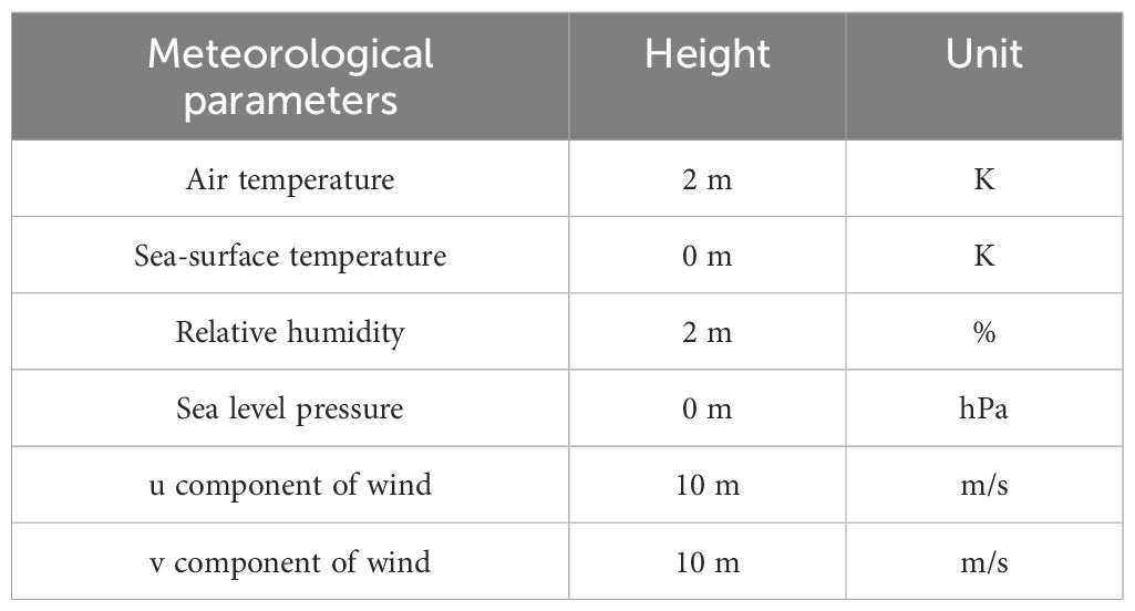
Table 1. Parameters obtained from ERA5.

In order to verify the accuracy of the ERA5 dataset, this paper uses the NCEP CFSv2 and MERRA2 datasets for cross-comparison. The comparison results are shown in Figure 1. The ERA5 dataset demonstrates relatively small differences compared to NCEP CFSv2 in terms of air temperature, wind speed, and sea level pressure, with RMSE of 0.58°C, 0.35 m/s, and 0.53 hPa, respectively. However, notable discrepancies emerge between ERA5 and NCEP CFSv2 in relative humidity and sea surface temperature, with RMSE values reaching 6.72% and 4.25°C. Since NCEP CFSv2 dataset is not observational measurements, it cannot serve as definitive evidence for the ERA5 dataset having substantial errors in relative humidity and sea surface temperature. To further investigate this, this study conducted comparative analyses using MERRA-2 dataset. As illustrated in Figure 1, MERRA-2 shows closer alignment with ERA5 in both relative humidity and sea surface temperature. The RMSE between MERRA-2 and ERA5 measures 3.25% for relative humidity and 1.08°C for sea surface temperature, whereas comparisons between MERRA-2 and NCEP CFSv2 yield higher RMSE values of 7.51% and 3.91°C, respectively. These results suggest that the ERA5 dataset demonstrates superior accuracy in relative humidity and sea surface temperature compared to the NCEP CFSv2 dataset.

Figure 1

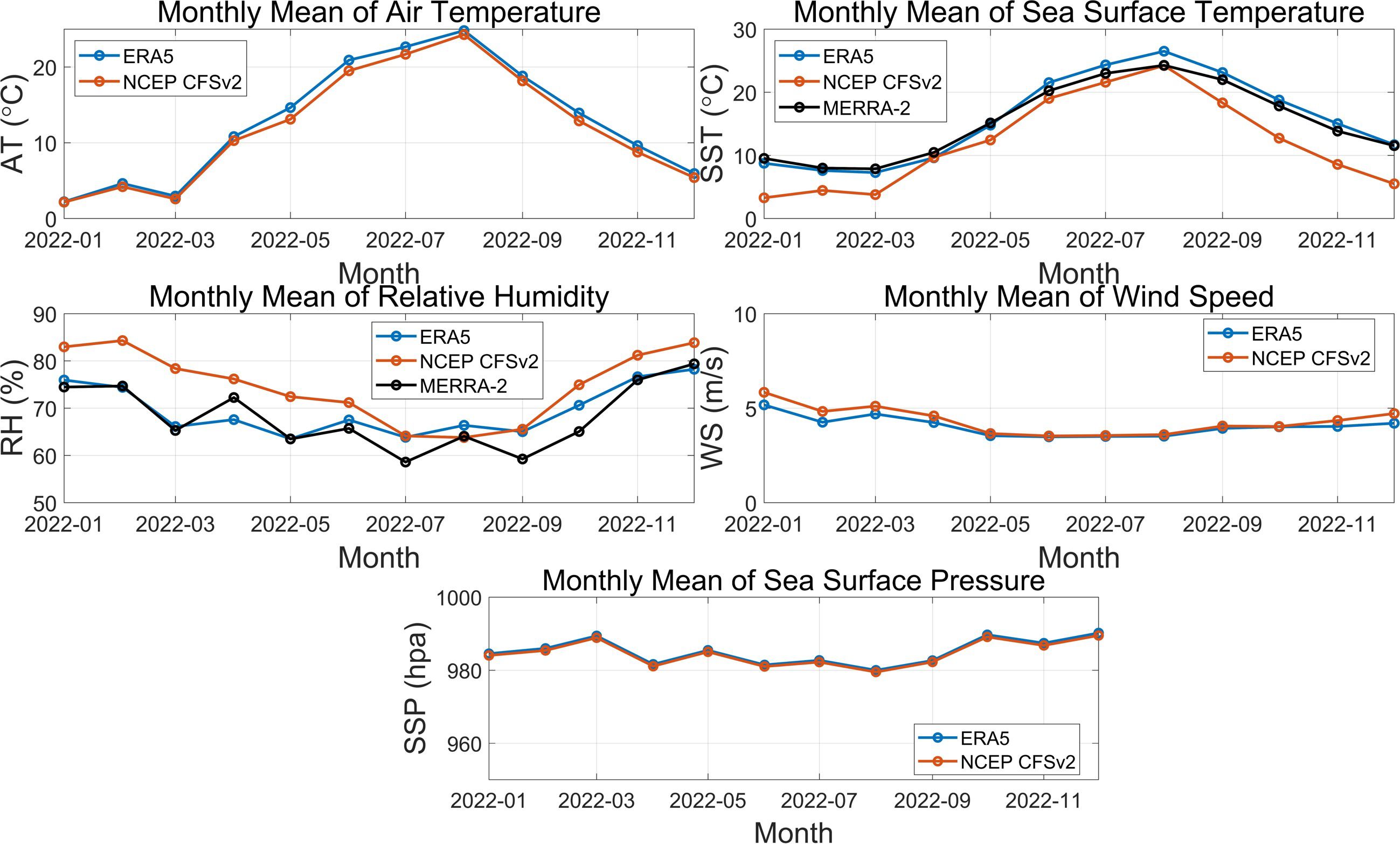
Figure 1. The comparison of NCEP CFSv2, MERRA-2 and ERA5 of monthly averages of air temperature, relative humidity, sea surface temperature, wind speed and sea surface pressure in the Black Sea region.

The validation of ERA5 data against the NCEP CFSv2 and MERRA-2 datasets demonstrates that the ERA5 dataset possesses sufficient accuracy.

2.2 Evaporation duct model

The evaporation duct prediction model is the main tool used to obtain the modified refractivity profiles (M profile) and EDH. The NAVSLaM model (Frederickson et al., 2000; Frederickson, 2015) is used in this paper. It utilizes the TOGA COARE 3.0 bulk flux algorithm to calculate the correlative scaling parameters of the Monin-Opukhov approach. The NAVSLaM model can be used to calculate the M profile and EDH by utilizing the air temperature, wind speed, sea level pressure, relative humidity and sea surface temperature.

The modified refractivity M is described by the following Equations 1:

$\begin{array}{ll}M=77.6\frac{P}{T}-5.6\frac{e}{T}+3.75\times {10}^5\frac{e}{T^2}+0.157z& (1)\end{array}$

where P is the total air pressure, unit is hPa, T is the air temperature, unit is K, e is the partial pressure of water vapour, unit is hPa and z is the height, unit is m.

In the NAVSLaM model, the vertical sections of the wind speed (u), temperature (T) and specific humidity (q) in the near-surface layer are obtained via the following Equations 2–4 (Babin and Dockery, 2002; Babin et al., 1997):

$\begin{array}{ll}u(z)=u(z_{0u})+\frac{u_{*}}{\kappa }\left[ln\right(\frac{z}{z_{0u}})-{\psi }_m(\frac{z}{L}\left)\right]& (2)\end{array}$

$\begin{array}{ll}T(z)=T(z_{0\theta })+\frac{{\theta }_{*}}{\kappa }\left[ln\right(\frac{z}{z_{0\theta }})-{\psi }_h(\frac{z}{L}\left)\right]-{\text{Γ}}_{d}z& (3)\end{array}$

$\begin{array}{ll}q(z)=q(z_{0q})+\frac{q_{*}}{\kappa }\left[ln\right(\frac{z}{z_{0q}})-{\psi }_h(\frac{z}{L}\left)\right]& (4)\end{array}$

where u(z), T(z) and q(z) are the wind speed, the air temperature and the relative humidity at height z, respectively. z_0u, z_0θ, and z_0q are the roughness heights of the wind speed, temperature, and specific humidity, respectively. u_∗, θ_∗ and q_∗ represent the Monin-Obukhov scaling parameters for the wind speed, temperature, and humidity, respectively. The values of z_0q, z_0θ, z_0u, u_∗, θ_∗ and q_∗ can be calculated using the TOGA COARE 3.0 bulk flux algorithm (Fairall et al., 2003). L is the Obukhov length. κ is Karman’s constant, and Γ_d is the dry adiabatic lapse rate. ψ_m and ψ_h are the stability correction functions of the wind speed and temperature, respectively. Under different stable atmospheric states, the stability correction functions of the wind speed and temperature are different. ζ = z/L is the Monin-Opukhov parameter, which reflects the thermodynamic atmospheric conditions. When the ASTD is zero, the atmosphere is considered neutral. If the difference is greater than zero, the atmosphere is stable. Conversely, if the difference is less than zero, the atmosphere is unstable.

Equation 1 shows that to obtain the modified refractive index profile, the vertical profile p(z) of atmospheric pressure and the water vapour partial pressure profile e must be determined. In the NAVSLaM model, the atmospheric pressure profile can be described by Equation 5.

$\begin{array}{ll}p(z_2)=p(z_1)exp\left(\frac{g(z_1-z_2)}{R{T}_v}\right)& (5)\end{array}$

where g represents acceleration due to gravity and z₁ is the observation height. z₂ is the height of the surface layer, and R is the gas constant for dry air. T_v is the average value of the virtual temperature at heights z₁ and z₂, in K.

The humidity and atmospheric pressure profile can be obtained from Equations 4, 5, and the water vapour partial pressure profile e can be obtained from Equation 6.

$\begin{array}{ll}e=\frac{qp}{ϵ+(1-ϵ)q}& (6)\end{array}$

where ϵ is a constant equal to 0.62.

The modified refractive index profile can be calculated from Equation 1 combined with the Equation 6. Assuming that the air temperature is 25°C, the sea-surface temperature is 30°C, the wind speed is 8 m/s, the relative humidity is 75%, and the atmospheric pressure is 1050 hPa, the corrected refractive index profile can be calculated via the NAVSLaM model, and the results are shown in Figure 2. The calculated strength of the evaporation duct and the EDH are 20.85 M-units and 15.4 m, respectively.

Figure 2

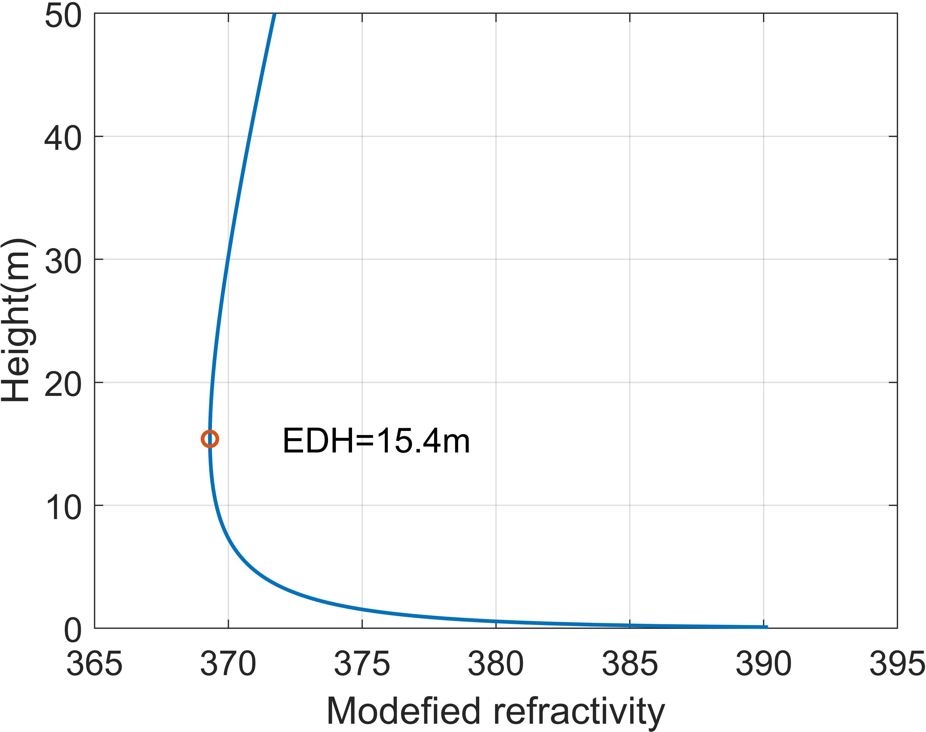
Figure 2. Modified refractivity profile estimated via the NAVSLaM model.

2.3 Parabolic equation method

Evaporation ducts can affect the performance of maritime communication and shipborne radar systems by influencing electromagnetic wave propagation. The parabolic equation (PE) method is applied to investigate the influence of evaporation ducts on electromagnetic wave propagation. The PE method is based on an approximation of the Helmholtz wave equation, and the scalar Helmholtz wave equation can be described as follows (Levy, 2000):

$\begin{array}{ll}\frac{{\partial }^2\psi }{\partial x^2}+\frac{{\partial }^2\psi }{\partial z^2}+k_0^2{n}^2\psi =0& (7)\end{array}$

where k₀ is the free space wavenumber, n(x,z) is the refractive index, ψ is a horizontally or vertically polarized electric or magnetic field, and x and z represent the distance and height coordinates, respectively.

The horizontally or vertically polarized electric or magnetic field ψ is replaced in the attenuation function in the paraxial direction x, as expressed in Equation 8:

$\begin{array}{ll}u(x,z)=exp(j{k}_{0}x)\psi (x,z)& (8)\end{array}$

The standard PE model shown in Equation 9 can be obtained by substituting the attenuation function (8) into the Helmholtz wave Equation 7:

$\begin{array}{ll}\frac{{\partial }^{2}u}{\partial x^2}+\frac{{\partial }^{2}u}{\partial z^2}+2j{k}_0\frac{\partial u}{\partial x}+k_0^2(n^2-1)u=0& (9)\end{array}$

The Fourier split step (FSS) is applied to establish the PE model. The FSS has been verified as stable and efficient (Sirkova, 2012) and has thus become the preferred method to solve problems related to long-distance tropospheric electromagnetic wave propagation. The FSS solution of the PE model can be obtained from Equation 10:

$\begin{array}{ll}u(x+\text{Δ}x,z)=\text{exp}[jk(n^2-1)\frac{\text{Δ}x}{2}]F^{-1}\left\{\text{exp}\right[-j{p}^2\frac{\text{Δ}x}{2k}\left]F\right\{u(x,z)\}\}& (10)\end{array}$

where p=ksinθ, θ is the height angle from the paraxial direction, △x represents the increment of the range, and F[·] and F⁻¹[·] represent the Fourier transform and the Fourier inverse transform, respectively.

3 Distribution of evaporation ducts in the Black Sea

3.1 Statistical analysis of the long-term mean EDH

The evaporation ducts in the Black Sea region are very unevenly distributed in different months and regions. As shown in Figure 3, the EDH is generally high during April and May. Specifically, the EDH in April is approximately 16.6 m, whereas in May, it is approximately 16.0 m. In June, the EDH is high in the north and low in the south. In June, the EDH in the northern Black Sea region is approximately 17.6 m, and the EDH in the southern region is approximately 10.7 m, with a large north-south difference. In the following section, the distribution characteristics of evaporation ducts in different regions of the Black Sea region in different months are explored. Figure 3 presents the monthly average EDH in the Black Sea region throughout the year, Figure 4 shows a line chart of the monthly average EDH in each region of the Black Sea throughout the year, and Table 2 presents the statistical characteristics of the EDH in each region of the Black Sea throughout the year.

Figure 3

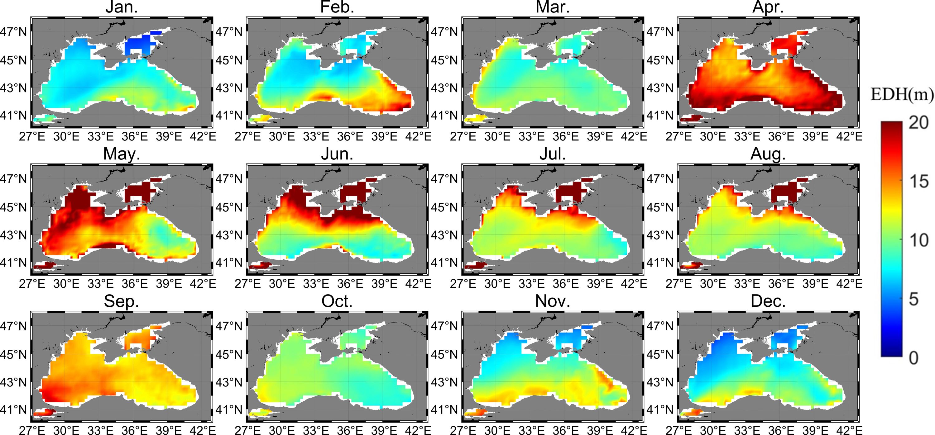
Figure 3. Spatial and temporal variations in EDH in the Black Sea.

Figure 4

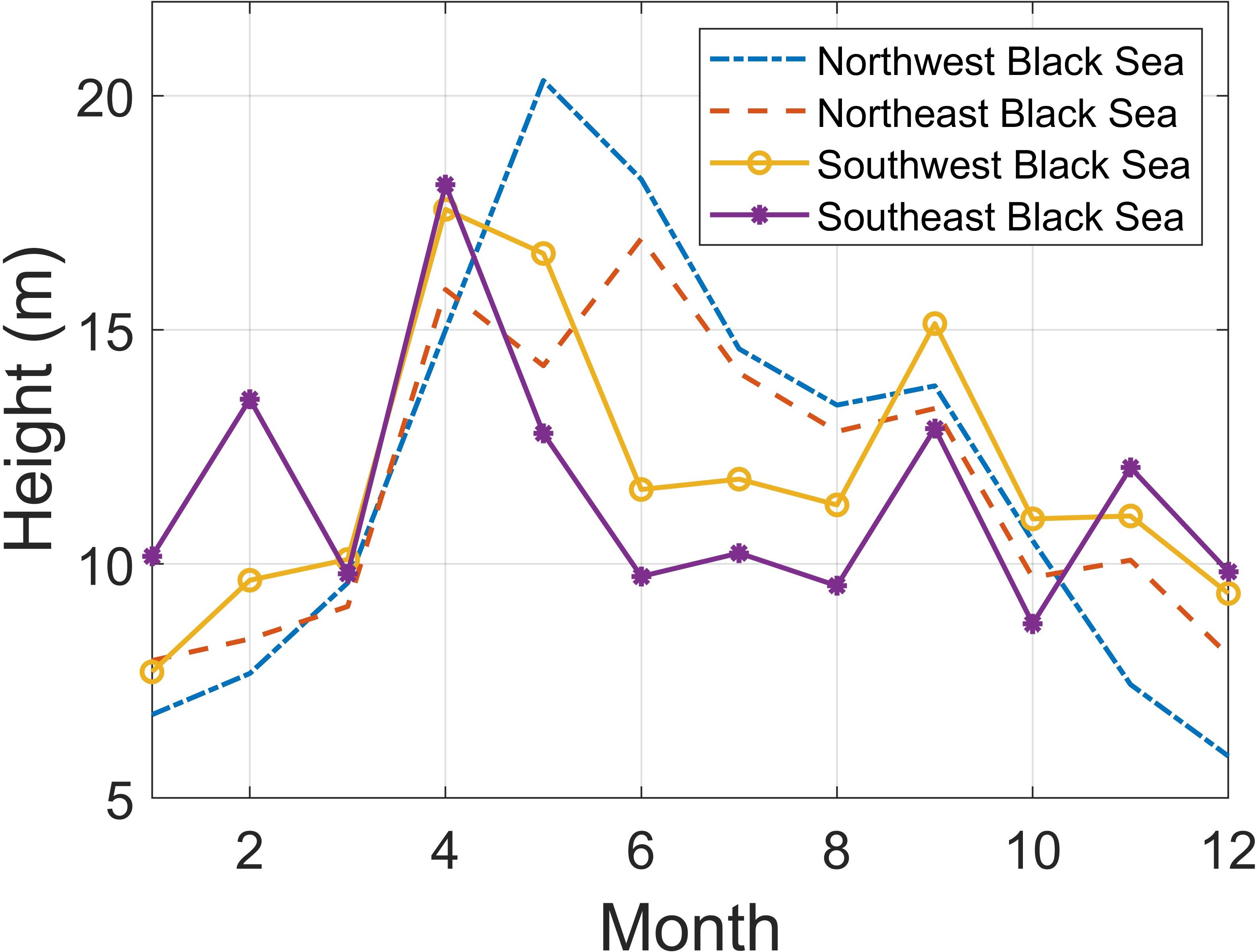
Figure 4. Monthly average EDH across different regions of the Black Sea.

Table 2

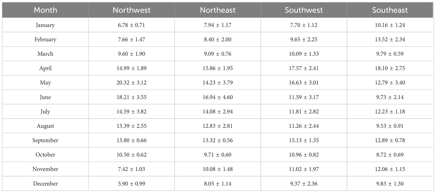
Table 2. EDH statistics in different Black Sea regions (mean ± standard deviation, m).

3.1.1 Northwest Black Sea

From Figure 3, the monthly average EDH in the northwestern Black Sea region is less than 10 m from January to March and November to December, and the monthly average EDH remains above 10 m from April to October. Specifically, the monthly average EDH reaches a maximum of 20.3 m in May. The seasonal variation pattern over the entire region is relatively obvious. The average EDH during spring and summer is approximately 15.18 m, whereas in autumn and winter, it is approximately 8.68 m. As illustrated in Figure 4, in the northwestern Black Sea region, the overall trend of the EDH is that the average height gradually increases from January, reaching a peak of 20.3 m in May. It then decrease following the May peak, rebounding by 0.4 m in September before reaching a minimum of 5.90 m in December. As shown in Table 2, the standard deviation of the EDH during autumn and winter across the entire northwestern region is relatively low, reaching a minimum of 0.62 m in October.

3.1.2 Northeast Black Sea

As shown in Figure 3, the average EDH in the northeastern Black Sea region from April to September is 12–17 m. The average EDH in the remaining months is mostly less than 10 m. Moreover, in the northeastern Black Sea region, the average EDH follows the pattern of high in spring and summer and low in autumn and winter. The average EDH in the region is 13.84 m in spring and summer and 9.58 m in autumn and winter. From Figure 4, in the northeastern Black Sea region, the EDH is high in spring and summer and low in autumn and winter, but there are fluctuations between seasons. Unlike that in the northwestern region, the average EDH in the northeastern region shows a downwards trend in summer and an upwards trend in winter. From April to May, the average EDH in the northeastern region decreased by 1.6 m. From January to March, the average EDH increased by 1.15 m. As shown in Table 2, from May to August, the standard deviation of the EDH in this region was 2.8-4.6 m. The standard deviation reached a maximum value of 4.6 m in June.

3.1.3 Southwest Black Sea

As shown in Table 2, the average EDH in the southwestern Black Sea region reaches a minimum of 7.70 m in January and a maximum of 17.57 m in April. The EDH in this region does not conform to the variation pattern of the average EDH in the northern region, which is high in spring and summer and low in autumn and winter. As illustrated in Figure 4, there are two peaks in the southwestern region, namely, in April (17.57 m) and September (15.13 m). In addition, the average EDH in winter is 7–10 m, which is greater than that in the northern region. With the arrival of spring, the average EDH in the region increases significantly. The average EDH in summer remains between 11 and 12 m. In autumn, the average EDH in September increases to 15.13 m. As shown in Table 2, the standard deviation of the EDH in this region is greater in February and from April to August and remains above 2 m. The standard deviation reaches a maximum of 3.17 m in June.

3.1.4 Southeast Black Sea

From Figure 3, the EDH in the southeastern Black Sea reaches a maximum of 18.10 m in April and a minimum of 8.72 m in October. The seasonal variation of the average EDH in the southeastern Black Sea is not obvious enough, lacking distinct high values in spring and summer and low values in autumn and winter. As illustrated in Figure 4, the average EDH in the region is relatively stable. Except that in April and October, the average EDH in other months fluctuates from 9–14 m. The standard deviation of the EDH in this area is smaller than that in other areas. As shown in Table 2, except in February and from April to June, the standard deviation of the EDH in this area is less than 2 m, and the distribution is relatively stable.

3.2 Physical mechanisms of the EDH distributions

Changes in meteorological elements have important impacts on the EDH. Therefore, analysing the spatiotemporal changes in meteorological elements in the Black Sea area is conducive to assessing the physical causes of the spatiotemporal changes in evaporation ducts. By utilizing ERA5 reanalysis data, the spatial and temporal distributions of the statistical characteristics of the wind speed, relative humidity, air temperature, sea surface temperature, and air-sea temperature difference in the Black Sea can be obtained.

Additionally, conducting a sensitivity analysis between the EDH and various meteorological elements is essential for clarifying their relationships. This analysis helps further reveal the physical causes behind the spatiotemporal changes in the evaporation ducts.

Figure 5 shows the monthly average wind speed in the Black Sea region in January, April, July and November. From Figure 5, the wind speed distribution in the Black Sea is relatively uniform. In January, northwest winds prevailed in the Black Sea region, with a high overall wind speed. Notably, the wind speeds in some areas reached more than 8 m/s. In April, the wind direction in the Black Sea was complex, with a west wind prevailing in the western Black Sea at an average speed of 5.5 m/s. In the central Black Sea, the wind direction changed from west to southwest, and the wind speed averaged 4.83 m/s. Overall, southwest winds prevailed in the eastern Black Sea. In July, northwest winds prevailed in the northwestern Black Sea, with an average wind speed of 4.11 m/s. Southwest winds prevailed in the southwest Black Sea, with an average wind speed of 4.42 m/s. In November, southeast winds prevailed in the western Black Sea, with an average wind speed of 5.39 m/s. During the study period, there was a small cyclone in the eastern Black Sea with a wind speed of 4.65 m/s.

Figure 5

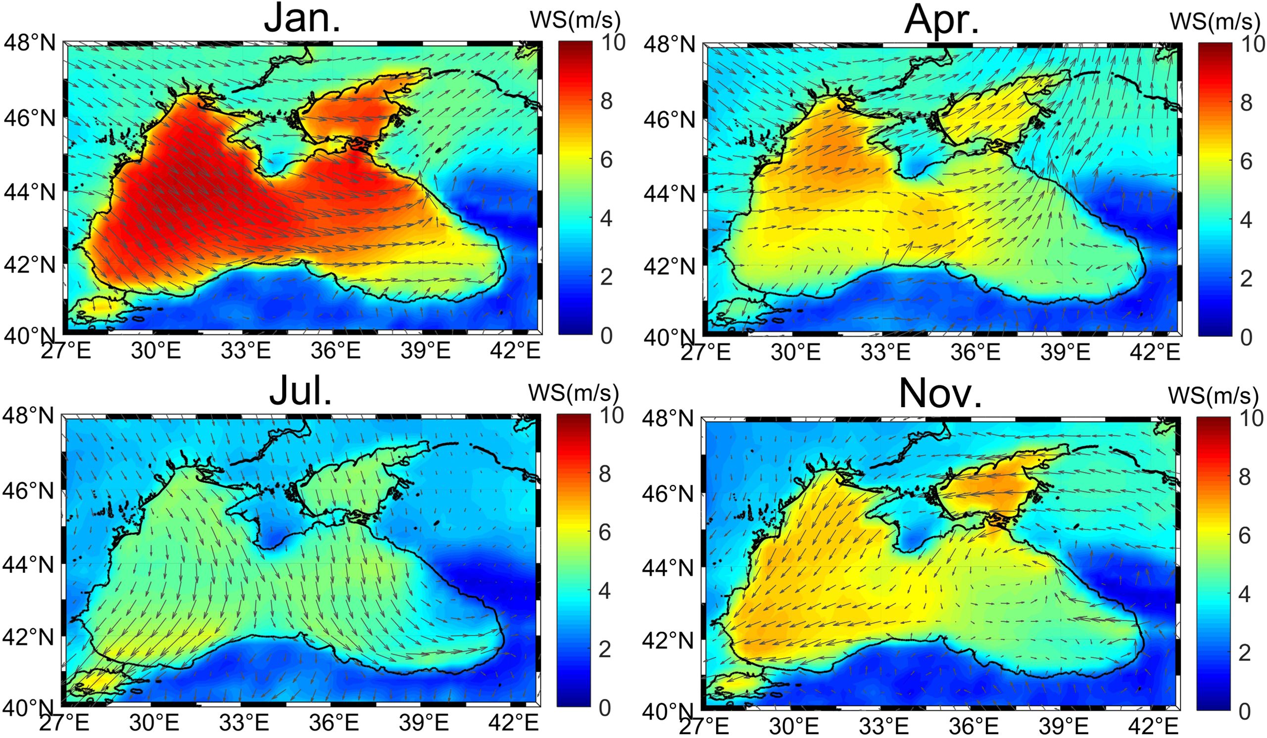
Figure 5. Monthly average variations in wind speed in the Black Sea region.

Changes in wind speed and direction in the Black Sea region have a certain impact on air temperature and relative humidity. Figures 6, 7 show the relative humidity and air temperature in the Black Sea region in January, April, July and November, respectively. In January, northwest winds prevailed in the Black Sea, blowing cold and dry air from the European continent to the Black Sea over the coasts of Bulgaria, Romania and Ukraine. The monthly average air temperature in the Black Sea decreased to 2.04°C, the lowest air temperature in the Black Sea region throughout the year. In addition, under the influence of the northwest wind, dry air on land was blown to the Black Sea, and the water vapour on the sea surface was transported to the eastern land portion of the Black Sea region. In April, the Black Sea was affected mainly by air currents transported from the coastlines of Bulgaria and Romania. As the temperature in Eastern Europe increased, the air currents transported warm air to the Black Sea, and the monthly average air temperature in the Black Sea increased to 10.79°C. There was a dry air mass northwest of the Black Sea. Combined with the wind direction in the Black Sea region in April, the dry air mass moved towards the sea, and the monthly average relative humidity in the sea further decreased. In July, the Black Sea was affected by two air currents along the Ukrainian coastline, blowing hot and dry air from Eastern Europe to the Black Sea, and the monthly average air temperature rose to 22.59°C. Affected by the mountainous terrain in Turkey, water vapour in the Black Sea gathered in the lower right area of the Black Sea region, forming a high-humidity area. In November, with the arrival of winter, the air temperature on land in Eastern Europe decreased, but the decrease in the air temperature in the Black Sea was relatively low, with a monthly average air temperature of 9.46°C. The Black Sea region as a whole presented high air temperatures over the seas and low air temperatures over land. There was a humid air mass in the northern Black Sea, and under the influence of the southeast wind, water vapour was transported to the northwestern Black Sea.

Figure 6

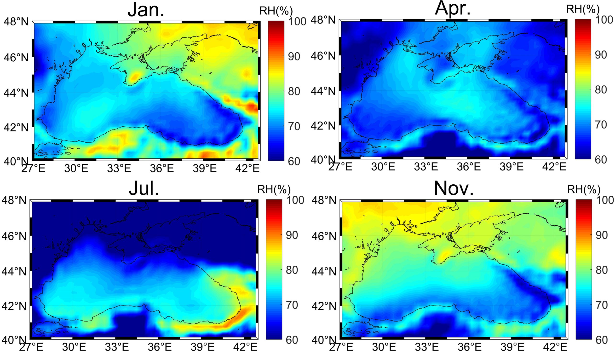
Figure 6. Monthly average variations in relative humidity in the Black Sea region.

Figure 7

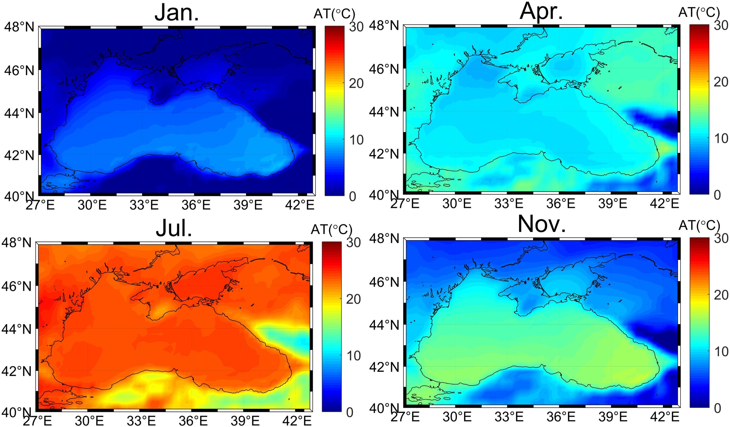
Figure 7. Monthly average variations in air temperature in the Black Sea region.

Figures 8, 9 show the monthly average sea surface temperature and the ASTD in the Black Sea region in January, April, July and November, respectively. On the basis of the results in Figures 7, 8, in the autumn and winter seasons, the air temperature in the Black Sea decreases rapidly, but the sea surface temperature decreases slowly. Therefore, the ASTD is large in the autumn and winter seasons. As shown in Figure 9, the monthly average ASTD in the Black Sea in January is -2.88°C, and the monthly average ASTD in November is -1.68°C, and the corresponding trends are both highly unstable. In April, the air temperature in the Black Sea region increases rapidly, but the sea surface temperature increases slowly. Therefore, in April, the air temperature in the Black Sea region is higher than the sea surface temperature, and the monthly average ASTD is 0.96°C, which is in a highly stable state.

Figure 8

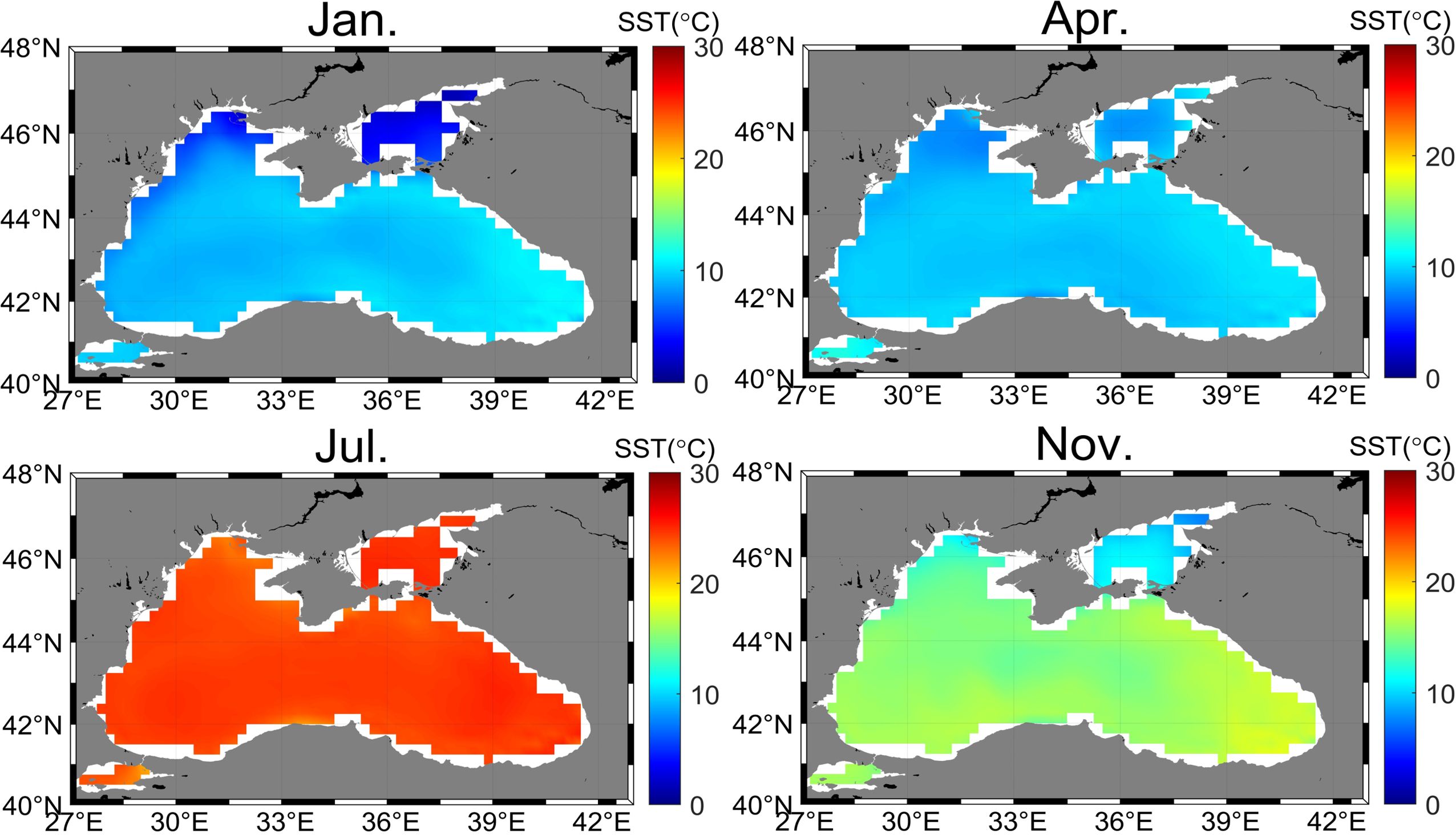
Figure 8. Monthly average variations in sea surface temperature in the Black Sea region.

Figure 9

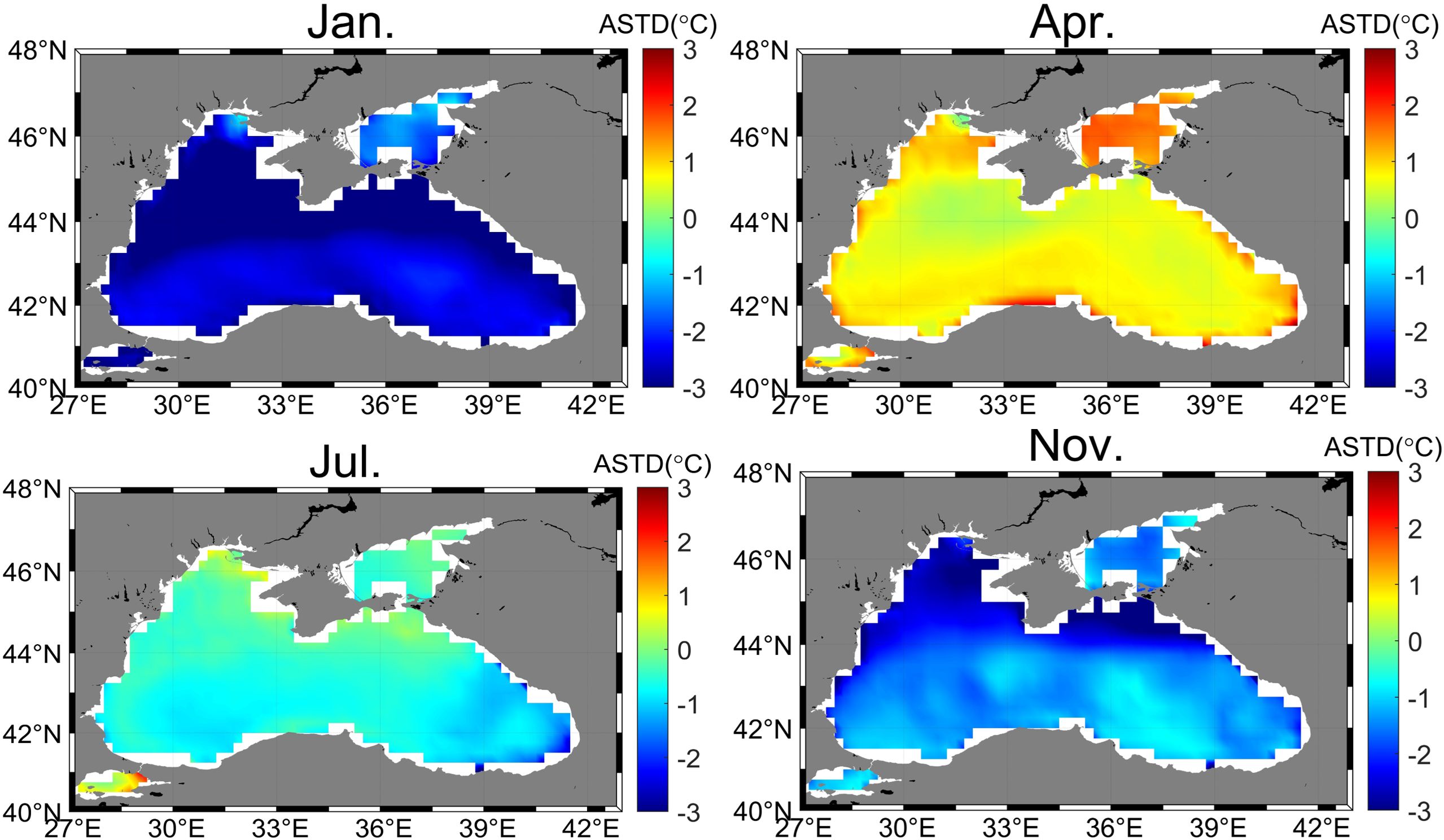
Figure 9. Monthly average variations in air-sea temperature difference in the Black Sea region.

To further reveal the physical mechanisms that influence the temporal and spatial distributions of evaporation ducts, a sensitivity analysis of the EDH to different meteorological parameters was conducted. Figure 10 shows different EDH curves as a function of air temperature and wind speed. In Figures 10a, b, it is assumed that the ASTD is 0.91°C (stable state) and -2°C (highly unstable state), which are the average values in April and November, respectively. Figure 10a shows that in a stable state, when the relative humidity is constant, the EDH usually increases with increasing air temperature or decreasing wind speed. When the relative humidity changes, a decrease in the relative humidity leads to a sharp increase in the EDH. Figure 10b shows that in a highly unstable state, when the relative humidity is constant, the EDH increases with increasing air temperature or wind speed. When the relative humidity changes, the EDH increases sharply with decreasing relative humidity.

Figure 10

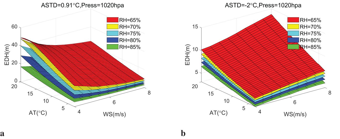
Figure 10. Sensitivity of the EDH to meteorological parameters. (a) Meteorological parameters for April. (b) Meteorological parameters for November.

The spatiotemporal characteristics of the air-sea temperature difference, wind speed and relative humidity in the Black Sea region in different months can be used to assess the physical mechanisms of the spatiotemporal distribution of the EDH in different regions of the Black Sea region, as described below.

3.2.1 Northwest Black Sea

As shown in Table 2, the EDH in the northwestern Black Sea region is relatively high in May and June. At these times, the ASTD northwest of the Black Sea are 0.39°C and 0.16°C, respectively, indicating a stable state. In May and June, the monthly average wind speeds in the northwestern Black Sea are 4.26 m/s and 4.45 m/s, respectively, which are relatively low values. In addition, the air temperature in this area is relatively high in May and June, at 15.55°C and 21.37°C, respectively. In addition, the relative humidity in this area is relatively low in May and June, with values of 60.43% and 66.84%, respectively. Therefore, under stable conditions, low wind speeds, low relative humidity and high air temperatures lead to a high EDH in this area in May and June.

3.2.2 Northeast Black Sea

As shown in Table 2, the northeastern Black Sea region is characterized by a high EDH in June. The ASTD is -0.053°C, indicating unstable conditions. The air temperatures and sea surface temperatures are 21.69°C and 21.81°C, respectively, both relatively high. Under unstable conditions, increasing temperatures lead to increased EDH. However, the relative humidity exceeds 75% in most months, which results in lower EDH than those in other regions.

3.2.3 Southwest Black Sea

As shown in Table 2, the EDH in the southwestern Black Sea region is highest in April, with a monthly average of 17.57 m. The ASTD is 0.78°C, indicating stable conditions. The average wind speed is 5.23 m/s, and the relative humidity is 68.84%, both of which are relatively low. These stable conditions contribute to the higher EDH in April than at other times.

In summer, autumn, and winter, the EDH are generally lower in the region, except in September. During September, the ASTD is -1.91°C, indicating strongly unstable conditions. The air temperature is 20.65°C, and the relative humidity is 66.75%, both contributing to an increase in EDH due to the presence of unstable conditions.

3.2.4 Southeast Black Sea

As shown in Table 2, the EDH in the southeastern Black Sea was relatively high in April, with a value of 18.10 m. In April, the air-sea temperature difference in the region was 0.87°C, reflecting a stable state. The average monthly wind speed in the region in April was 4.44 m/s, which was relatively low. In addition, the relative humidity in the region was 69.73% in April, which was relatively low. In a stable state, low wind speed and relative humidity lead to a higher EDH. As shown in Table 2, the EDH was relatively low from May to December in this region. During this period, the air-sea temperature difference in the region was less than 0, indicating an unstable state. In addition, during this period, the wind speed in the region was less than 4.5 m/s, which was relatively low. Moreover, the relative humidity was relatively high, and except for the relative humidity of 69% in September, that in the other months was greater than 70%. In an unstable state, low wind speed and high relative humidity lead to a lower EDH.

4 Impact of evaporation ducts on electromagnetic wave propagation

Evaporation ducts trap electromagnetic waves, which in turn cause abnormal propagation of electromagnetic waves, resulting in over-the-horizon propagation of electromagnetic waves. In addition, the uneven distribution of evaporation waveguides will also affect the propagation of electromagnetic waves (Yang et al., 2024c). Therefore, evaporation ducts have an important impact on electromagnetic wave propagation at sea. Although hybrid ducts (e.g., surface-based or elevated ducts) also can affect electromagnetic wave propagation, their occurrence probability is significantly low (typically below 20%) (Shi et al., 2023; Sirkova, 2015). Therefore, this study focuses exclusively on the impact of evaporation ducts. In this section, the impact of evaporation ducts on electromagnetic wave propagation at sea is investigated through APM simulations. The impact of evaporation ducts on the marine channel is analysed in detail during the period when the Moskva ship was discovered. The APM model combines the PE method and the geometric optics method. The PE method has an advantage at small elevation angles, while the relatively fast geometric optics method can reduce execution time. These are the reasons for combining them. Specifically, the PE method is mainly applied in the evaporation duct area. Considering these features, the APM model is thus employed to analyze the impact of the evaporation duct on electromagnetic wave propagation, as its combined approach can effectively meet the requirements of such analysis.

On April 13, 2022, the Russian warship Moskva exploded in the Black Sea and sank a few days later. The cause of the explosion of the Moskva ship was that it was hit by two Ukrainian R-360 Neptune anti-ship missiles. Norin et al. (2023) noted that the radar that discovered the Moskva ship was located at 46.6°N, 31.0°E. The coordinates where the ship was discovered were 45.4°N and 30.75°E. Figure 11 shows the electromagnetic wave propagation link of the radar that discovered the Moskva ship. The blue circle represents the radar location, and the red five-pointed star represents the Moskva ship. The green grid points are the ERA5 reanalysis data grid points, and the red grid points are the grid points involved in the propagation process.

Figure 11

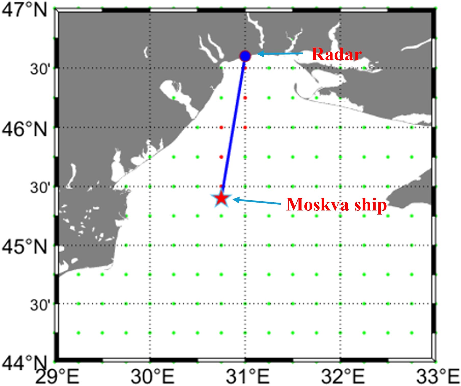
Figure 11. Radar (blue circle) and Moskva ship (red star) location diagram.

Norin et al. (2023) noted that the Moskva ship was discovered by radar at approximately 13:00. Therefore, in the analysis of electromagnetic wave propagation characteristics, the EDH is set to the nonuniform EDH on the link between the radar and the Moskva ship at 13:00 on April 13, 2022. This study selects representative classic parameters (Wang et al., 2020; Shi et al., 2023, 2015) as the APM parameters. These parameters are consistent with practical applications and have demonstrated good stability in existing research, ensuring a certain degree of reproducibility and credibility.The parameter settings of the APM model are shown in Table 3. Under the condition of a nonuniform EDH for the link between the radar and the Moskva ship at 13:00 on April 13, 2022, the electromagnetic wave propagation characteristics are shown in Figure 12.

Table 3

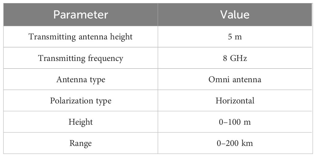
Table 3. Parameters for the APM model.

Figure 12

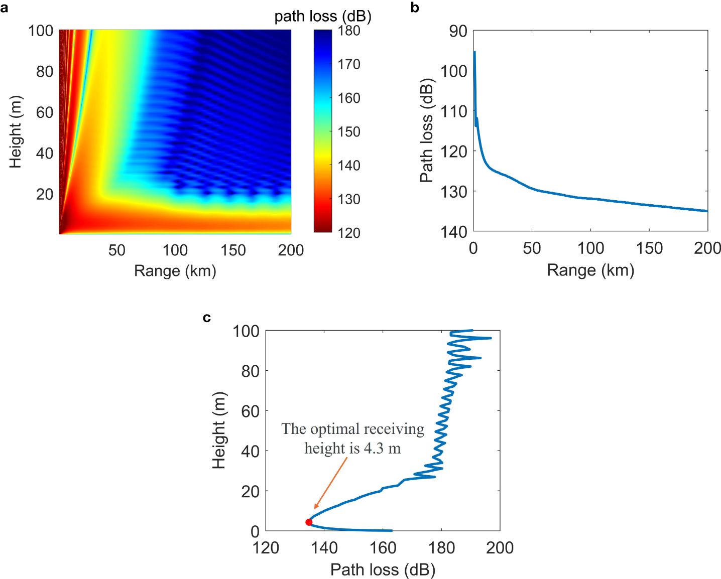
Figure 12. Simulation of electromagnetic wave propagation under nonuniform EDH conditions on the radar and Moskva ship link at 13:00 on April 13, 2022. (a) Propagation loss. (b) Receiving height of 5 m. (c) Receiving distance of 200 km.

From Figure 12a, the electromagnetic wave energy first propagates upwards, and then part of the electromagnetic wave energy is trapped in the evaporation duct layer, realizing over-the-horizon propagation. As shown in Figure 12b, when the receiving antenna height is 5 m, for the evaporation duct, within the range of 20 km, the path loss increases rapidly with increasing distance. In the range of 20–200 km, the path loss increases slowly with increasing distance, and the path loss is approximately 149 dB at 200 km. Figure 12c shows the variation in the electromagnetic wave propagation path loss with distance at 200 km. For the evaporation duct, the electromagnetic wave propagation path loss first decreases with increasing receiving height, reaching a minimum value of 135.3 dB at a height of 4.3 m, and then the path loss increases with increasing receiving height. When the altitude exceeds 20.2 m, path loss fluctuates with increasing altitude but generally tends to increase.

Figure 13a shows the daily variation in link propagation loss between the radar and Moskva ship on April 13, 2022. As shown in Figure 13a, the daily variation in the link propagation loss between the radar and the Moskva ship is quite dramatic. The overall trend is that from 0:00 onward, the propagation loss continues to increase, reaching a peak value (212.1 dB) at 5:00. From 5:00 to 12:00, the propagation loss decreases, reaching a minimum (134.6 dB) at 12:00. After 12:00, the propagation loss increases. In general, on April 13, 2022, when the propagation loss reached a minimum at approximately 12:00, the radar detection performance improved, and the probability of target detection increased. At approximately 5:00 and after 16:00, the propagation loss was high, the radar detection performance decreased, and the probability of target detection decreased. Norin et al. (2023) noted that the Moskva ship was discovered by radar at approximately 13:00. At this time, the link was in a period of high radar detection performance.

Figure 13

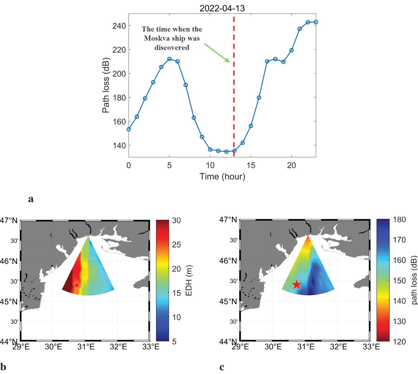
Figure 13. Distribution and changes of EDH and propagation loss at April 13, 2022. (a) Temporal variation of path loss on the day of the Moscow ship was attacked, April 13th, 2022. (b) Spatial distributions of EDH at 13:00, April 13, 2022. (c) Spatial distributions of path loss at 13:00, April 13, 2022.

From Figure 13b, within the radar detection sector, the EDH generally tends to be high on the left and low on the right. A high EDH corresponds to low propagation loss. Therefore, as shown in Figure 13c, within the radar detection sector, the propagation loss also tends to be low on the left and high on the right. In areas with low propagation losses, the radar detection performance is best. In areas with high propagation losses, the radar detection performance is comparatively worse. Within the radar detection sector, the detection performance in the left area is best, and the detection performance in the right area is worst. In addition, there is a certain detection blind spot on the right. The location where the ship was discovered is in an area with excellent radar detection performance.

5 Conclusion

In this study, the long-term distribution patterns of evaporation ducts in the Black Sea region were investigated, the nonuniform effects on maritime channel characteristics were explored, and the corresponding roles in the Moskva incident were analyzed. The main findings of this paper are summarized as follows:

(1) The EDH in the Black Sea region demonstrates pronounced spatial-seasonal variability, with contrasting north-south gradients across seasons. During summer, the northern EDH exceeds the southern value by 4.31 m, whereas during winter, it displays an inverse pattern, with the southern EDH surpassing the northern value by 2.58 m. In spring and autumn, the north-south difference is less than 1 m. Furthermore, regional analysis reveals seasonal variability in the northern Black Sea. Notably, high values occur during spring and summer, reaching 14.01 and 15.01 m, respectively, whereas low levels are observed in autumn and winter, at 10.81 and 7.45 m, respectively.

(2) Sensitivity analysis reveals that the ASTD and relative humidity constitute the key factors influencing the EDH, whereas other meteorological elements have relatively minor impacts. In the Black Sea region, seasonal fluctuations in the ASTD demonstrate relatively small variation amplitude, with prevailing unstable conditions across most seasons. Consequently, the seasonal variability in the EDH in the Black Sea region is driven primarily by dynamic changes in relative humidity, which serve as the predominant physical mechanism governing these fluctuations.

(3) Nonuniformities in evaporation ducts significantly affect marine channels. Analysis of the Moskva incident revealed that different evaporation duct conditions can cause variations in path propagation loss within the marine channel of up to 100 dB. Favorable evaporation duct conditions can substantially enhance the performance of electromagnetic systems in marine channels.

These results directly inform maritime radar deployment strategies, emphasizing the importance of temporal targeting. Accurately grasping the time window can significantly enhance the performance of the electromagnetic system. Future work should extend this framework to other marginal seas and incorporate real-time meteorological inputs for adaptive electromagnetic system design. Our methodology bridges climatological analysis and engineering applications, offering a template for region-specific evaporation duct studies in support of reliable maritime operations.

Data availability statement

The original contributions presented in the study are included in the article/supplementary material. Further inquiries can be directed to the corresponding author.

Author contributions

CF: Software, Formal analysis, Data curation, Validation, Visualization, Writing – original draft, Writing – review & editing, Methodology, Investigation. SW: Conceptualization, Formal analysis, Resources, Writing – review & editing, Methodology. CH: Funding acquisition, Writing – review & editing, Project administration. FY: Funding acquisition, Writing – review & editing. YS: Funding acquisition, Validation, Writing – review & editing, Investigation. KY: Supervision, Writing – review & editing.

Funding

The author(s) declare that financial support was received for the research and/or publication of this article. This work was supported in part by the National Natural Science Foundation of China under Grant 62341133 and Grant 12304498, in part by the Fundamental Research Funds for the Central Universities under Grant D5000240070 and in part by the National Science Foundation of Shandong Province under Grant ZR2023QA116, in part by the Student Innovation Funds for Northwestern Polytechnical University (Taicang) under Grant TCCX240102.

Conflict of interest

The authors declare that the research was conducted in the absence of any commercial or financial relationships that could be construed as a potential conflict of interest.

Generative AI statement

The author(s) declare that no Generative AI was used in the creation of this manuscript.

Publisher’s note

All claims expressed in this article are solely those of the authors and do not necessarily represent those of their affiliated organizations, or those of the publisher, the editors and the reviewers. Any product that may be evaluated in this article, or claim that may be made by its manufacturer, is not guaranteed or endorsed by the publisher.

References

Babin S. M. and Dockery G. D. (2002). Lkb-based evaporation duct model comparison with buoy data. J. Appl. Meteorol. Climatol. 41, 434–446. doi: 10.1175/1520-0450(2002)041<0434:LBEDMC>2.0.CO;2

Crossref Full Text | Google Scholar

Babin S. M., Young G. S., and Carton J. A. (1997). A new model of the oceanic evaporation duct. J. Appl. Meteorol. Climatol. 36, 193–204. doi: 10.1175/1520-0450(1997)036<0193:ANMOTO>2.0.CO;2

Crossref Full Text | Google Scholar

Barrios A., Patterson W., and Sprague R. (2002). Advanced propagation model (apm) version 2.1. 04 computer software configuration item (csci) documents. (San Diego, California, USA: Space and Naval Warfare Systems Center), 0704–0188.

Google Scholar

Cheng Y., Zha M., Qiao W., He H., Wang S., Wang S., et al. (2024). An improved remote sensing retrieval method for elevated duct in the South China sea. Remote Sens. 16, 2649. doi: 10.3390/rs16142649

Crossref Full Text | Google Scholar

Cheng Y., Zha M., You Z., and Zhang Y. (2021). Duct climatology over the South China sea based on European center for medium range weather forecast reanalysis data. J. Atmos. Solar-Terrestrial Phys. 222, 105720. doi: 10.1016/j.jastp.2021.105720

Crossref Full Text | Google Scholar

Fairall C. W., Bradley E. F., Hare J., Grachev A. A., and Edson J. B. (2003). Bulk parameterization of air–sea fluxes: Updates and verification for the coare algorithm. J. Climate 16, 571–591. doi: 10.1175/1520-0442(2003)016<0571:BPOASF>2.0.CO;2

Crossref Full Text | Google Scholar

Frederickson P. A. (2015). “Further improvements and validation for the navy atmospheric vertical surface layer model (NAVSLaM),” in 2015 USNC-URSI Radio Science Meeting (Joint with AP-S Symposium) (Vancouver, British Columbia, Canada: IEEE), Vol. 242. doi: 10.1109/USNC-URSI.2015.7303526

Crossref Full Text | Google Scholar

Frederickson P., Davidson K., and Goroch A. (2000). Operational bulk evaporation duct model for MORIAH version 1.2 (Monterey, CA, USA: Nav. Postgraduate School).

Google Scholar

Hersbach H., Bell B., Berrisford P., Hirahara S., Horányi A., Muñoz-Sabater J., et al. (2020). The era5 global reanalysis. Q. J. R. Meteorol. Soc. 146, 1999–2049. doi: 10.1002/qj.3803

Crossref Full Text | Google Scholar

Huang L., Zhao X., Liu Y., Yang P., Ding J., and Zhou Z. (2022). The diurnal variation of the evaporation duct height and its relationship with environmental variables in the south China sea. IEEE Trans. Antennas Propag. 70, 10865–10875. doi: 10.1109/TAP.2022.3191160

Crossref Full Text | Google Scholar

Jeske H. (1973). “State and limits of prediction methods of radar wave propagation conditions over sea,” in Modern Topics in Microwave Propagation and Air-Sea Interaction: Proceedings of the NATO Advanced Study Institute held at Sorrento, Italy, ed. Zancla A. (Dordrecht: Springer Netherlands), 130–148. doi: 10.1007/978-94-010-2681-913

Crossref Full Text | Google Scholar

Kang K.-M. (2020). Evaluating a single column model blending algorithm using casper measurements. Monterey, California, USA: Naval Postgraduate School.

Google Scholar

Levy M. (2000). Parabolic equation methods for electromagnetic wave propagation Vol. 45 (London, UK: IET). doi: 10.1049/PBEW045E

Crossref Full Text | Google Scholar

Ma J., Wang J., and Yang C. (2022). Long-range microwave links guided by evaporation ducts. IEEE Commun. Mag. 60, 68–72. doi: 10.1109/MCOM.002.00508

Crossref Full Text | Google Scholar

Musson-Genon L., Gauthier S., and Bruth E. (1992). A simple method to determine evaporation duct height in the sea surface boundary layer. Radio Sci. 27, 635–644. doi: 10.1029/92RS00926

Crossref Full Text | Google Scholar

Norin L., Wellander N., and Devasthale A. (2023). Anomalous propagation and the sinking of the Russian warship Moskva. Bull. Am. Meteorol. Soc. 104, E2286–E2304. doi: 10.1175/BAMS-D-23-0113.1

Crossref Full Text | Google Scholar

Ozgun O., Sahin V., Erguden M. E., Apaydin G., Yilmaz A. E., Kuzuoglu M., et al. (2020). Petool v2. 0: Parabolic equation toolbox with evaporation duct models and real environment data. Comput. Phys. Commun. 256, 107454. doi: 10.1016/j.cpc.2020.107454

Crossref Full Text | Google Scholar

Qiu Z., Hu T., Wang B., Zou J., and Li Z. (2022). Selection optimal method of evaporation duct model based on sensitivity analysis. J. Atmos. Ocean. Technol. 39, 941–957. doi: 10.1175/JTECH-D-21-0133.1

Crossref Full Text | Google Scholar

Raptis K. (2012). Climatological factors affecting electromagnetic surface ducting in the Aegean sea region. Monterey, California, USA: Naval Postgraduate School.

Google Scholar

Shi Y., Wang S., Yang F., and Yang K. (2023). Statistical analysis of hybrid atmospheric ducts over the northern South China sea and their influence on over-the-horizon electromagnetic wave propagation. J. Mar. Sci. Eng. 11, 669. doi: 10.3390/jmse11030669

Crossref Full Text | Google Scholar

Shi Y., Yang K., Yang Y., and Ma Y. (2015). Influence of obstacle on electromagnetic wave propagation in evaporation duct with experiment verification. Chin. Phys. B 24, 54101. doi: 10.1088/1674-1056/24/5/054101

Crossref Full Text | Google Scholar

Sirkova I. (2012). Brief review on PE method application to propagation channel modeling in sea environment. Open Eng. 2, 19–38. doi: 10.2478/s13531-011-0049-y

Crossref Full Text | Google Scholar

Sirkova I. (2015). Duct occurrence and characteristics for Bulgarian black sea shore derived from ecmwf data. J. Atmos. Solar-Terrestrial Phys. 135, 107–117. doi: 10.1016/j.jastp.2015.10.017

Crossref Full Text | Google Scholar

Twigg K. L. (2007). A smart climatology of evaporation duct height and surface radar propagation in the Indian Ocean. Monterey, California, USA: Naval Postgraduate School.

Google Scholar

Wang Q. (2019). Estimation of refractivity conditions in the marine atmospheric boundary layer from range and height measurement of X-band EM propagation and inverse solutions. Columbus, Ohio, USA: The Ohio State University.

Google Scholar

Wang Q., Alappattu D. P., Billingsley S., Blomquist B., Burkholder R. J., Christman A. J., et al. (2018). Casper: Coupled air–sea processes and electromagnetic ducting research. Bull. Am. Meteorol. Soc. 99, 1449–1471. doi: 10.1175/BAMS-D-16-0046.1

Crossref Full Text | Google Scholar

Wang Q., Burkholder R. J., Yardim C., Xu L., Pozderac J., Christman A., et al. (2019). Range and height measurement of x-band em propagation in the marine atmospheric boundary layer. IEEE Trans. Antennas Propag. 67, 2063–2073. doi: 10.1109/TAP.2019.2894269

Crossref Full Text | Google Scholar

Wang S., Han J., Shi Y., Yang K., Huang C., and Yang F. (2020). “The influence of antenna height on microwave propagation in evaporation duct,” in Global Oceans 2020: Singapore–US Gulf Coast, vol. 1–5. (Biloxi, MS, USA: IEEE). doi: 10.1109/IEEECONF38699.2020.9389404

Crossref Full Text | Google Scholar

Wang S., Yang K., Shi Y., and Yang F. (2022). Observations of anomalous over-the-horizon propagation in the evaporation duct induced by typhoon Kompasu, (202118). IEEE Antennas Wirel. Propag. Lett. 21, 963–967. doi: 10.1109/LAWP.2022.3153389

Crossref Full Text | Google Scholar

Wang S., Yang K., Shi Y., Yang F., and Zhang H. (2023a). Observed over-the-horizon propagation characteristics and evaporation duct inversion during the entire process of tropical cyclone Mulan, (202207). IEEE Trans. Antennas Propag. 71, 5322–5334. doi: 10.1109/TAP.2023

Crossref Full Text | Google Scholar

Wang S., Yang K., Shi Y., Yang F., Zhang H., and Ma Y. (2023b). Prediction of over-the-horizon electromagnetic wave propagation in evaporation ducts based on the gated recurrent unit network model. IEEE Trans. Antennas Propag. 71, 3485–3496. doi: 10.1109/TAP.2023.3240998

Crossref Full Text | Google Scholar

Wang S., Yang K., Shi Y., Zhang H., Yang F., Hu D., et al. (2023c). Long-term over-the-horizon microwave channel measurements and statistical analysis in evaporation ducts over the yellow sea. Front. Mar. Sci. 10. doi: 10.3389/fmars.2023.1077470

Crossref Full Text | Google Scholar

Wauer B., Wang Q., Alvarenga O., Yamaguchi R., Kalogiros J., Alappattu D. P., et al. (2018). “Observations of optical turbulence in the marine atmospheric surface layer during casper-west,” in Laser Communication and Propagation through the Atmosphere and Oceans VII (San Diego, California, USA: SPIE), 116–130. doi: 10.1117/12.2321258

Crossref Full Text | Google Scholar

Wei Y., Gao M., Tian D., Guo L., Li J., Yang L., et al. (2022). A model for calculating electromagnetic scattering from target in evaporation duct. IEEE Antennas Wirel. Propag. Lett. 21, 2312–2316. doi: 10.1109/LAWP.2022.3190013

Crossref Full Text | Google Scholar

Xu L. (2019). Multi-frequency atmospheric refractivity inversion dissertation. Columbus, Ohio, USA: The Ohio State University.

Google Scholar

Xu L., Yardim C., Mukherjee S., Burkholder R. J., Wang Q., and Fernando H. J. S. (2021). Frequency diversity in electromagnetic remote sensing of lower atmospheric refractivity. IEEE Trans. Antennas Propag. 70, 547–558. doi: 10.1109/TAP.2021.3090828

Crossref Full Text | Google Scholar

Yang C., Shi Y., Wang J., and Feng F. (2022). Regional spatiotemporal statistical database of evaporation ducts over the South China sea for future long-range radio application. IEEE J. Select. Top. Appl. Earth Observ. Remote Sens. 15, 6432–6444. doi: 10.1109/JSTARS.2022.3197406

Crossref Full Text | Google Scholar

Yang N., Song D., Su D., Lu T., Sun L., and Wang T. (2024a). The influence of sea surface temperature from ecmwf reanalysis data on the non-uniformity of evaporation duct. IEEE Geosci. Remote Sens. Lett. 21, 1–5. doi: 10.1109/LGRS.2024.3408795

Crossref Full Text | Google Scholar

Yang N., Su D., Sun L., Lu T., Song D., and Wang T. (2024b). The horizontal inhomogeneity of the evaporation duct based on surface bulk measurements over the South China sea. IEEE Trans. Antennas Propag. 72, 7916–7926. doi: 10.1109/TAP.2024.3438360

Crossref Full Text | Google Scholar

Yang C. and Wang J. (2022). The investigation of cooperation diversity for communication exploiting evaporation ducts in the South China sea. IEEE Trans. Antennas Propag. 70, 8337–8347. doi: 10.1109/TAP.2022.3177509

Crossref Full Text | Google Scholar

Yang N., Zou X., Sun L., Su D., and Wang T. (2024c). The non-uniformity characteristics of the evaporation duct in the South China sea based on cldas data. Front. Mar. Sci. 10. doi: 10.3389/fmars.2023.1326975

Crossref Full Text | Google Scholar

Zhang C., Qiu Z., Fan C., Song G., Wang B., Hu T., et al. (2023). Research on a multimodel fusion diagnosis method for evaporation ducts in the East China sea. Sensors 23, 8786. doi: 10.3390/s23218786

PubMed Abstract | Crossref Full Text | Google Scholar

Zhang Q., Yang K., and Shi Y. (2016). Spatial and temporal variability of the evaporation duct in the Gulf of Aden. Tellus A: Dynam. Meteorol. Oceanogr. 68, 29792. doi: 10.3402/tellusa.v68.29792

Crossref Full Text | Google Scholar