Abstract
In marine engineering, polymer layers are anti-seepage barrier materials. The mechanical interaction between marine sand and polymer layer significantly affects overall structural stability. In this study, direct shear tests at different temperatures in the marine environment are simulated to evaluate the shear behavior of marine sand and polymer layer interface, and a database is developed. Based on the experimental data, the study employs the Back propagation Neural Network (BPNN), Genetic Algorithm and Particle Swarm Optimization BPNN, and convolutional neural network (CNN) models, which are trained and tested. The findings show that the CNN algorithm significantly outperforms other models in terms of prediction accuracy and efficiency. Sensitivity analysis shows that temperature, shear displacement, normal stress, and particle size have influence on interfacial shear strength, and the impact of normal stress is the greatest. In addition, an empirical formulation is proposed to provide tools for those without machine learning. Based on the research results, the deep learning CNN model developed in the study can accurately predict the shear strength of the interface between marine sand and the polymer layer, which provides an effective tool for the design and optimization of marine engineering.
1 Introduction
In marine engineering, marine sand is widely distributed in near-shore waters and is often used as a natural foundation material for offshore structures in coral reef areas and island regions (El-Saadony et al., 2023; Huang et al., 2024b; Rowe and Islam, 2009; Sangam, 2001; Singh et al., 2009). Polymer layers are often used in various types of marine engineering structures due to their functional characteristics such as impermeability and reinforcement (Divya et al., 2012; Lin et al., 2024; Song et al., 2024). Nevertheless, in practical engineering, the shear strength of the marine sand-polymer layer interface (MSPLI) is relatively low. It is also highly susceptible to temperature variations in marine environments (Akpinar and Benson, 2005). Elevated temperatures can lead to a decrease in the mechanical properties of the interface, thereby increasing the potential for marine structural instability (Chao et al., 2023c; Karademir and Frost, 2021; Yin et al., 2021). In addition, temperature changes also affect the contact state between the marine sand particles and their bonding properties with the polymer layer, which further weakens the mechanical properties of the interface (Gao and Ye, 2023; Reddy et al., 2022; Ye and Gao, 2024) Therefore, it is of great engineering significance to study the shear strength of the MSPLI under the effect of temperature to guarantee the long-term stability and safety of marine engineering structures (Hamidi and Garousi, 2024; Liang et al., 2025).
The straight shear test is a common method to study the mechanical behavior of the MSPLI (Chao et al., 2024c). For example, Bilgin et al. investigate the effect of temperature on the MSPLI by using a large-scale straight shear device and find that an increase in temperature leads to the softening of polymer layers (Chao et al., 2023b; Cheng et al., 2023; Wang et al., 2025), which reduces the interfacial mechanical properties (Bilgin and Stewart, 2006; Li et al., 2024). In addition, Khan et al. find that the interfacial shear strength increased significantly with the increase of normal stress through the interfacial shear test between marine sand and polymer layer (Chao et al., 2024f; Khan and Latha, 2025). Chen et al. analyze the relationship between the interfacial displacement and sand strain under different normal and shear stress amplitudes through static and dynamic single-shear tests and find that the change of the shear displacement affects the stress-strain response of the MSPLI, which further increases the interfacial (Chen et al., 2025; Ye et al., 2022; Zhang et al., 2023a). The study shows that the mechanical behavior of the interface is affected by many factors, except for temperature, normal stress, temperature, and shear displacement, which more strongly affects the mechanical behavior of the interface (Gao and Ye, 2024; Ye et al., 2019). Although the straight shear test can provide reliable experimental data and reveal the interfacial shear behavior, it still has some limitations (Chao et al., 2024a). First, the test is costly and time-consuming, making it difficult to be widely used in engineering practice (Fan et al., 2023; Sevim and Demir, 2019; Zhou et al., 2022). The polymer layers used in actual projects are usually finalized at the late stage of design (Zhao et al., 2023a), which limits the applicability of the test results (Xiao et al., 2024; Zhang et al., 2023b). Secondly, the experimental environmental conditions (e.g., temperature, etc.) are difficult to control accurately (Gong et al., 2025a; Guo et al), which leads to uncertainty in the test results and thus affects the reliability of the engineering design (Chao et al., 2022; Dong et al., 2017; Zheng et al., 2024a). Therefore, there is an urgent need to develop an efficient prediction method that can comprehensively consider multiple influencing factors and reduce the experimental cost while ensuring accuracy so as to make up for the shortcomings of physical experiments.
In order to address the limitations of direct shear tests, the artificial intelligence method provides an innovative approach to studying the MSPLI (Chao et al., 2024f; Li et al., 2025). Researchers are increasingly using machine learning models to make predictions (Chao et al., 2024d; Zhao et al., 2023b). For example, Liu et al. use the backpropagation neural network (BPNN) method to evaluate slope instability (Ding et al., 2024; Liu et al., 2024; Shao et al., 2024). Jin et al. use the BPNN optimized by genetic algorithm (GA-BPNN) model to predict high-performance concrete (Jin et al., 2024). Xiao et al. propose an enhanced BPNN prediction model based on a particle swarm optimization (PSO) algorithm (Xiao et al., 2023). It is shown that these models are able to quickly predict interface mechanical behavior through a data-driven approach and exhibit high prediction accuracy and efficiency (Xiao and Xu, 2024). Nevertheless, there are still some limitations of machine learning methods (Shi et al., 2023). For example, Katoch et al. studied genetic algorithms (GA) and found that their optimization process is computationally expensive and prone to fall into local optimal solutions (Gong et al., 2025b; Katoch et al., 2021). Hajihassani et al. pointed out that although PSO converges quickly, it is sensitive to initial parameters and has a weak search ability in high-dimensional space (Hajihassani et al., 2018). In contrast, deep learning models, especially CNN, offer significant advantages for complex interface problems. Convolutional neural networks can automatically learn hierarchical features from raw data, thereby capturing more complex nonlinear relationships between input parameters. This ability makes convolutional neural networks particularly suitable for predicting interface mechanical behavior in geotechnical engineering, whereas traditional machine learning models often struggle to achieve similar accuracy and scalability (Shu et al., 2025). Although these optimization methods improve the accuracy of the model to some extent, they still rely on traditional machine learning frameworks (Sun et al., 2019). It is difficult to fundamentally solve the problem of feature extraction by relying on expert experience (Shi et al., 2025). Since feature selection for machine learning models usually relies on manual labor, it may lead to loss of information or the introduction of subjective bias, which in turn affects the accuracy and reliability of the model (Chauhan and Singh, 2018; Xu et al., 2024). Although the feature set selected by the expert can reflect the key factors, the lack of automation and comprehensiveness may not cover all potentially influential factors, which limits the expressive power of the model (Chao et al., 2024b, 2024e; Ye and Gao, 2024). In addition, when dealing with large-scale, high-dimensional data, traditional machine learning models have high computational and storage requirements, and the prediction accuracy and generalization ability may be insufficient (Kamath et al., 2018; Lai, 2019; Paterakis et al., 2017). Therefore, researchers are gradually turning to deep learning techniques to overcome the shortcomings of traditional machine learning and improve prediction accuracy and generalization ability.
In recent years, convolutional neural network (CNN) in deep learning technology has been widely used in the engineering field. CNN can automatically extract multiple layers of features from raw data, which reduces the reliance on manual feature engineering (Chao et al., 2024g; Ren et al., 2024; Schmidhuber, 2015). Meanwhile, it has a strong nonlinear fitting ability and generalization performance, which is suitable for dealing with complex engineering problems (Chao et al., 2023a; Ren et al., 2016). For example, in the field of construction materials and engineering, Li et al. propose a one-dimensional CNN method based on soft sorting, which significantly improves the accuracy of concrete creep prediction by converting tabular data into multi-channel images and exploiting the spatial locality property of CNN (Chao et al., 2025; Li et al., 2023). The results show that CNN can mine deeper information when processing and analyzing data characterized by spatial localization, thereby enhancing prediction accuracy and reliability (Chao et al., 2024c; Gao and Ye, 2024). In the field of civil engineering, Zhang et al. propose a scanning electron microscope (SEM) image recognition method based on CNN. By inputting SEM images into the CNN model, the powerful feature extraction capability is utilized (Zhang et al., 2024). The microstructure characteristics of the concrete-rock interface transition zone (ITZ) are successfully identified. The accuracy of the quantitative analysis of ITZ thickness and crack distribution has significantly improved (Cui et al., 2024). These studies further demonstrate the superior performance of CNN in image processing and feature recognition, which demonstrates their strong potential in processing complex data and image analysis (Shi et al., 2025; Wang et al., 2023; Yang et al., 2025). Nevertheless, although CNN has achieved remarkable results in several engineering fields, its application in predicting marine sand and polymer layer interface behavior has not been fully explored.
The mechanical response at the MSPLI under varying temperatures is analyzed in this research. Under different temperature conditions, direct shear tests are carried out on the MSPLI with the particle size range of 1mm-2mm and 2mm-4mm to obtain the interface mechanical behavior data. A database is built based on the test results, and various machine learning models, including deep learning CNN, are employed to train and predict the data. Through comparative analysis of the accuracy and generalization ability of different models, CNN is determined to be the best model.
2 Physical test methodology
2.1 Materials
Marine sand and polymer layers were selected as experimental materials, as shown in Figure 1 and Figure 2. In order to assess the effect of particle size on shear strength, the sea sand was categorized into two groups of particle sizes, 1–2 mm and 2–4 mm, using the sieving method. The particle size of 1-2mm was denoted as S1, and the particle size of 2-4mm was denoted as S2 for subsequent description. Marine sand and polymer layer related parameters were shown in Table 1.
Figure 1
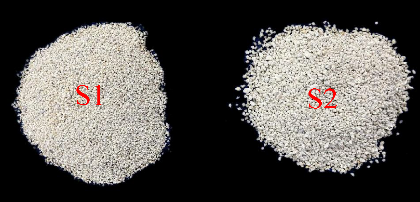
Marine sand sample.
Figure 2
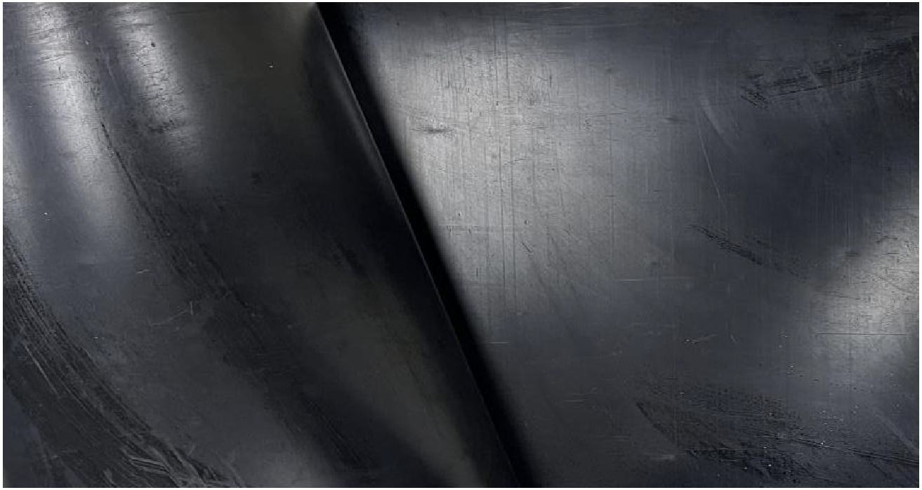
Polymer layer.
Table 1
| Thickness (mm) | Density (g*cm-3) | Ultimate tensile strength (kN*m-1) | Limit elongation(%) |
|---|---|---|---|
| 2.0 | 0.942 | 29.3 | 12 |
Polymer layer related parameters.
2.2 Experimental procedure
As shown in Figure 3, the monotonic shear test was performed using a large temperature-controlled straight shear apparatus equipped with a temperature-controlled chamber that can control the temperature in the range of 20 °C to 150 °C and a shear box with dimensions of 300 mm × 300 mm × 150 mm. Prior to the test, the polymer layer was cut to 280 mm × 460 mm and fixed to the lower part of the shear box. The marine sand samples were filled into the shear box in a total of six layers, with each layer having a thickness of 2 cm. In the test, the marine sand and polymer layer samples with different grain sizes were placed in the shear box. The test temperature was controlled at 5 °C, 20 °C, 40 °C, 60 °C, and 80 °C. The normal stresses of 15 kPa, 25 kPa, and 50 kPa were applied to the upper and lower shear boxes, respectively. The shear rate was uniformly set to 1 mm/min. The shear path started from the initial position 0 and was carried out along paths a to b until the interfacial shear stress reached the peak. The instrument was connected to computer software to record the test data in real time, including shear stress and shear displacement. These data were used to analyze how temperature and particle size influence the shear mechanical properties at the MSPLI.
Figure 3
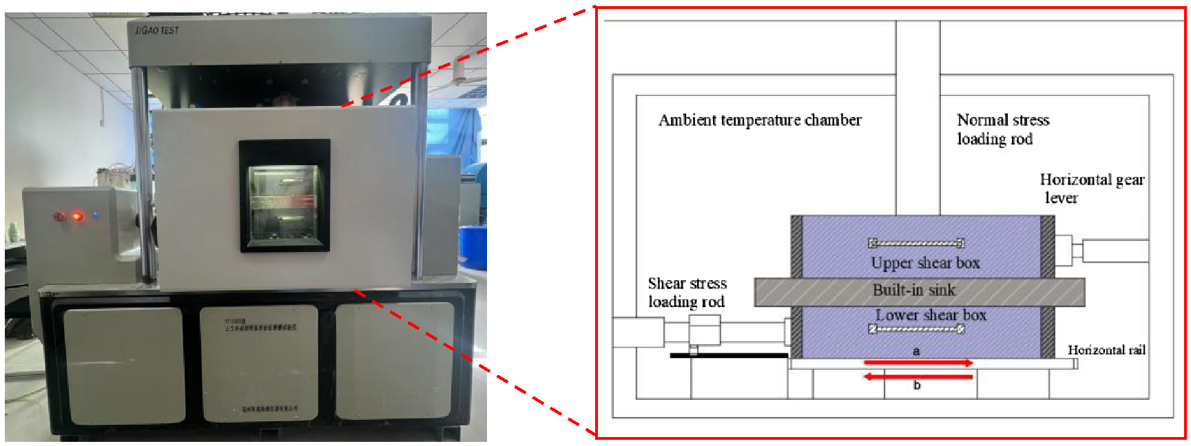
Shear box and shear path.
3 Methodology
3.1 Machine learning and deep learning algorithms
In the study, three machine learning algorithms and one deep learning algorithm are used to construct and optimize the models. These algorithms include BPNN, GA-BPNN, PSO-BPNN, and CNN. The advantages and disadvantages of each algorithm are compared as shown in Table 2. A brief description of these machine learning algorithms and the deep learning algorithm will follow:
Table 2
| Algorithm | Strengths | Limitations |
|---|---|---|
| BPNN | Non-linear modeling, function approximation |
Sensitive to architecture, prone to overfitting |
| GA-BPNN | Global search, no gradient required | Slow convergence, needs parameter tuning |
| PSO-BPNN | Simple, fast convergence, global search |
Can get trapped in local optima |
| CNN | Excellent for image and signal tasks, feature extraction | Requires large datasets, computationally intensive |
Comparison table of advantages and disadvantages of optimization algorithms.
3.1.1 BPNN
BPNN is an artificial neural network based on a back propagation algorithm. It receives data from the input parameters through the input layer and passes them to the hidden layer. Then weights and nonlinearly transform the input signals through the network weights and activation functions to produce the output results. The BPNN model used in the study contains four input layers (shear displacement, normal stress, temperature, and particle size), one output layer (shear stress), and five hidden layers. The model uses a logarithmic S-shaped function as the activation function. A back propagation neural network is created using the newff function to optimize the initial weights and thresholds. While combining the early-stop method to prevent overfitting, we systematically explore the adaptability of different combinations of network structures for shear stress prediction. Although the method has the advantages of simple modeling and strong nonlinear fitting ability, it suffers from the problems of easy to falling into local optimum and limited generalization ability, which become the motivation for the subsequent introduction of optimization algorithms.
3.1.2 GA
GA is an optimization algorithm that mimics the natural evolutionary process and searches for an optimal solution through operations such as selection, crossover, and mutation. In GA, an initial population is generated by initialization. Then the merit of each individual is evaluated using a fitness function. Based on the fitness value, the good individuals are selected for reproduction. New individuals are generated by crossover and mutation operations. Finally, the iterative process of selection, crossover, and mutation continues until the stopping criterion, such as the maximum number of iterations or an acceptable solution, is reached. GA has a wide range of applications in optimization and search problems. They demonstrate powerful search capabilities and adaptability, especially in complex problem spaces and situations that cannot be solved by traditional methods. In this study, GA is combined with a deep BPNN network and the genetic operator settings are optimized by parameter sensitivity analysis, so that the prediction model takes into account both global exploration and local convergence ability. Although GA-BPNN enhances the prediction performance of the model, its higher computational complexity and sensitivity to parameter adjustment still need attention.
3.1.3 PSO
PSO is an optimization algorithm based on swarm intelligence that simulates the behavior of biological groups such as birds or fish. In PSO, each candidate solution is treated as a particle that moves through the search space with the direction and speed of motion influenced by individual historical optimality and group historical optimality. The particle adjusts its position according to its current position and velocity update rules to find the optimal solution. The key advantages of PSO are that it is simple and easy to implement, has no gradient information, has global search ability, and has fast convergence. It is widely used in function optimization, neural network training, and other optimization problems. Dynamic inertia weight factors are introduced into the PSO update rule to balance the exploration and exploitation capabilities and significantly improve the model training speed and robustness. Nevertheless, PSO may still fall into local optimality, especially in the case of uneven data distribution, which requires multiple initializations to improve stability.
3.1.4 CNN
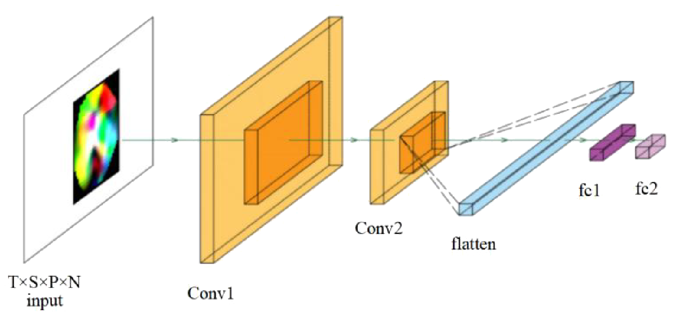
As depicted in Figure 4, CNN is a deep learning framework that employs convolutional and pooling layers, activation functions, and fully connected layers to process and extract features from the data. The convolutional layer performs local sensing to capture features by sliding the convolutional kernel over the input data. The activation function introduces nonlinearities to enhance the expressive ability of the model. The pooling layer reduces the data dimensions and computation by down sampling, while the fully connected layer performs further processing of the extracted features to accomplish the final prediction task. In the experiments of this paper, a CNN model containing two convolutional layers, two ReLU activation functions, and one fully connected layer is constructed for the regression task of the data, which exhibits excellent prediction accuracy and robustness. The input tensor is divided by time step to capture the parameter trends and achieve high accuracy prediction without manual feature extraction. Although CNN suffers from the problems of a complex model and high requirements on the amount of training samples, its superior generalization ability provides a new direction for solving engineering nonlinear problems.
Figure 4
CNN convolutional neural network diagram.
3.2 Model parameter configuration
3.2.1 Hyperparameter optimization
Hyperparameter optimization plays a crucial role in enhancing the performance of machine learning models, as varying configurations can lead to notable differences in both training efficiency and predictive accuracy. In the study, GA and PSO are used to optimize the hyperparameters of BPNN to improve the performance of the model. The purpose is to ensure that the algorithm can converge efficiently and improve the prediction accuracy. The key parameters in the optimization process of GA and PSO are set reasonably. As shown in Table 3, the population size (pop_num) is set to 5 in the GA optimization process to reduce the computational cost while maintaining the exploration capability of the solution space. The genetic generation (gen) is set to 50 to ensure the adequacy of optimization. The selection function parameter (normGeomSelect) is set to 0.09 so that individuals with higher fitness have a higher probability of being selected. The crossover function parameter (arithXover) is set to 2 to increase the diversity of solutions. The variation function parameter (nonUnifMutation) is set to [2,50,3] to enhance the global search ability and prevent premature convergence. The optimal solution tolerance (maxGenTerm) is set to 50 to ensure that the appropriate search can still be performed after the optimal solution is found, and to improve the stability of the solution. On the other hand, the learning factor (c1, c2) is set to 4.494 in the PSO optimization process to balance the effects of individual and group experience on particle velocity. The maximum position (popmax) and minimum position (popmin) are set to 1.0 and -1.0, respectively, to limit the search range of the particles. The population size (size pop) is set to 5 to balance computational efficiency and global search capability. The number of population updates (maxgen) is set to 50 to ensure sufficient iteration of the optimization process. The number of training times (epochs) is set to 100 to ensure that the neural network fully learns the data features. Overall, the reasonable hyperparameter settings enable both GA and PSO to effectively optimize the performance of the BPNN model. This approach enhances convergence efficiency and mitigates the risk of overfitting to a certain degree. Ultimately, the prediction accuracy of the model is significantly improved, which shows good potential for application in predicting the shear strength of MSPLI in marine engineering.
Table 3
| Hyperparameters | Parameter name | Range of values |
|---|---|---|
| GA | Population size(pop_num) | 5 |
| Genetic generations(gen) | 50 | |
| Selection function parameter(normGeomSelect) | 0.09 | |
| Crossover function parameter (arithXover) | 2 | |
| Mutation function parameter(nonUnifMutation) | [2,50,3] | |
| Optimal solution tolerance(maxGenTerm) | 50 | |
| PSO | Learning factors (c1, c2) | 4.494 |
| Maximum position (popmax) | 1.0 | |
| Minimum position (popmin) | -1.0 | |
| Population size (sizepop) | 5 | |
| Population update times (maxgen) | 50 | |
| Training iterations (epochs) | 100 |
Parameter settings for GA and PSO optimized BPNN.
Figure 5 demonstrates the performance comparison between GA and PSO based on Root Mean Square Error (RMSE) during the optimization process. The horizontal axis represents the number of iterations, which ranges from 0 to 50. the vertical axis represents the RMSE value, which reflects the magnitude of the model prediction error. Figure 5 shows that as the number of iterations increases, the RMSE values for both GA and PSO decline progressively, demonstrating the effectiveness of both algorithms in minimizing prediction error. It is worth noting that PSO converges significantly faster than GA and can achieve lower RMSE values in fewer iterations. It shows that PSO is more efficient in searching in space and can approach the optimal solution faster. Specifically, the PSO algorithm has a rapidly decreasing RMSE value at the beginning of the iteration and continues to decrease slowly in subsequent iterations, eventually stabilizing at around 1. The GA algorithm, on the other hand, also rapidly decreases the RMSE value at the beginning of the iteration. However, the decrease is relatively slow and stabilizes after about 20 iterations and eventually stabilizes at about 3. Comparison results show that PSO exhibits higher efficiency and better convergence performance in the optimization process.
Figure 5
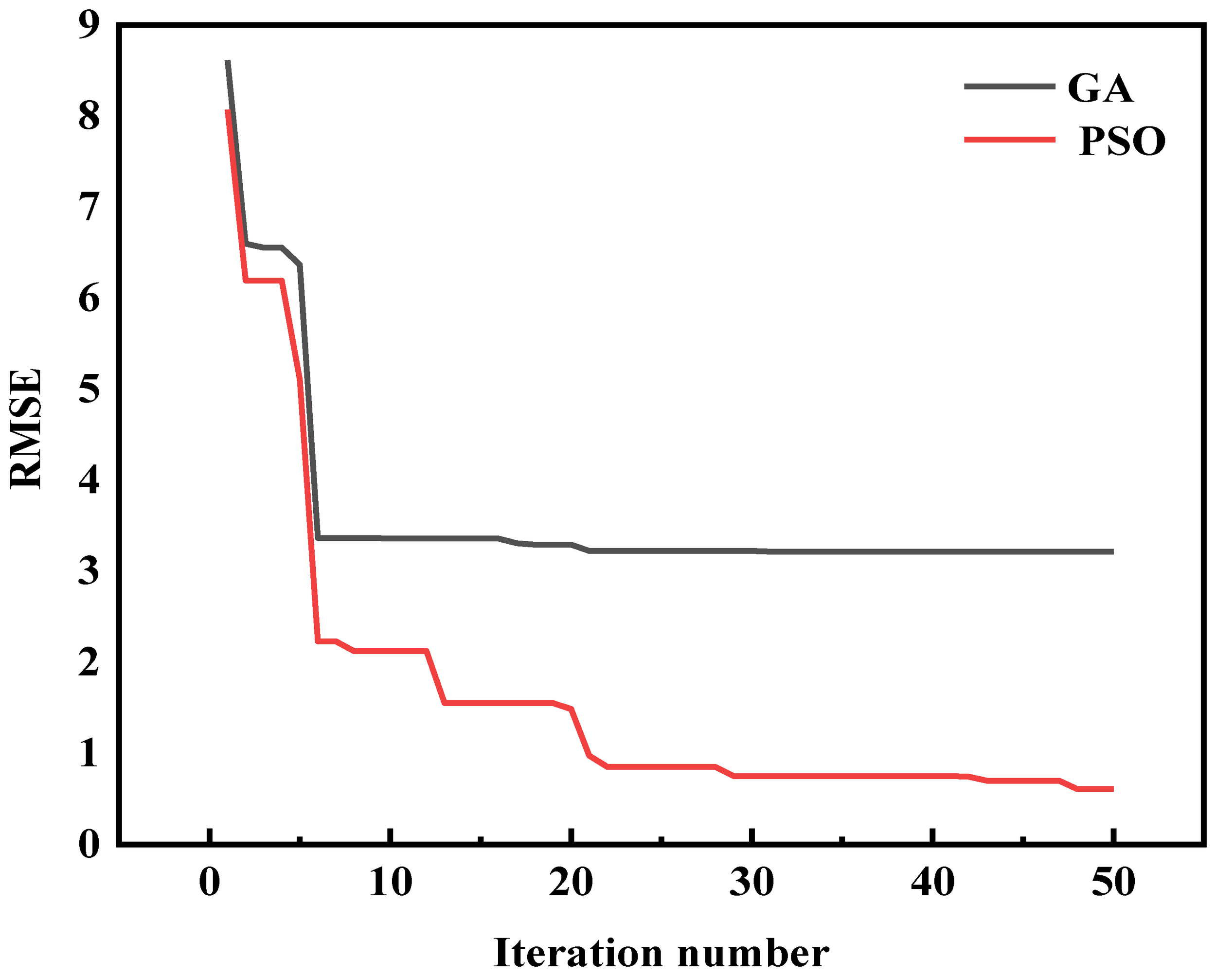
Number of RMSE iterations for GA and PSO.
3.2.2 CNN model parameters
This work establishes a one-dimensional convolutional neural network (1D-CNN) model to evaluate the temperature-dependent behavior of shear strength at the MSPLI. The inputs to the model include four features, namely normal stress, shear displacement, temperature, and particle size, and aim to reveal the nonlinear relationship between these factors and interfacial shear strength. The CNN model extracts local features through a convolutional layer, which learns the complex relationship between the input features and the target variable (shear strength) through a fully connected layer. As shown in Table 4, the model consists of multiple layers, each with parameter settings designed to efficiently extract key features of the input data and perform regression prediction.
Table 4
| Layer type | Parameter name | value |
|---|---|---|
| input layer | Input Shape | (100,4) |
| Convolutional layer 1 | Number of filters | 64 |
| Convolution kernel size | 3 | |
| activation function | ReLU | |
| Convolutional Layer 2 | Number of filters | 64 |
| Convolution kernel size | 3 | |
| activation function | ReLU | |
| Flatten layer | Flatten the multi-dimensional data into one-dimensional data | |
| Fully connected layer | Number of neurons | 50 |
| output layer | Number of neurons | 1 |
Parameter settings of CNN.
Specifically, the shape of the input layer is (100, 4), and each sample contains 100 time steps and 4 features, which ensure that the model can take full advantage of the timing information in the data. The convolution layer 1 contains 64 filters, and the convolution kernel size is 3. The activation function is ReLU, which can effectively extract local features and avoid the gradient disappearance problem. Convolutional Layer 2 is similar to Convolutional Layer 1 in that it enhances the model ability to capture complex patterns by further extracting advanced features. The flattened layer converts the multi-dimensional output of the convolutional layer into a one-dimensional vector, which is then passed to a fully connected layer with 50 neurons using the ReLU activation function to capture nonlinear relationships. Finally, the output layer contains 1 neuron dedicated to the regression task and outputs the predicted interfacial shear strength. During the training, the Adam optimizer and MSE loss function are employed in the model. After 50 epochs of training, the model shows high prediction accuracy and robustness in both the training set and the test set.
3.3 Establishment of database and data processing
In order to study the shear strength at the marine sand and polymer layer under different temperature conditions, a dataset containing 5102 data sets is established. The database includes five variables: temperature, particle size, normal stress, shear stress, and displacement. All input and output variables are normalized (Equation 1):
Where is the original data value, is the normalized data value, min is the smallest value in the data, and max is the largest value in the data set.
The summary statistics of variables in the database are shown in Table 5. The temperature ranges from 0 °C to 80 °C, the particle size is divided into three categories: fine, medium, and coarse, the normal stress ranges from 10 kPa to 300 kPa, and the shear stress ranges from 5 kPa to 150 kPa, and the displacement ranges from 0 mm to 50 mm. Data processing includes data cleaning, normalization, and data set splitting to ensure data quality and suitability for machine learning modeling.
Table 5
| Argument | Type | Minimum value | Maximum value | Mean value | Standard deviation |
|---|---|---|---|---|---|
| Temperature(°C) | Numerical type | 0 | 80 | 30 | 15 |
| Normal stress (KPa) | 10 | 300 | 155 | 75 | |
| Shear stress (KPa) | 5 | 150 | 77.5 | 37.5 | |
| Displacement (mm) | 0 | 50 | 25 | 12.5 | |
| Particle size (mm) | Nominal type | fine | coarse | – | – |
Statistical table of factors affecting the shear strength of the polymer layer interface.
3.4 Predictive performance assessment index
During the construction and tuning phases, the model performance is assessed based on selected evaluation indicators. In this study, the following two main assessment indicators are used:
1. The Root Mean Square Error (RMSE) measures the spread of prediction errors, defined as the standard deviation between forecasted and observed values, as shown in Equation 2. A smaller RMSE value indicates a lower prediction error and a more accurate model.
In this formula, n is the total number of samples, yi is the observed value, and fi is the predicted value.
2. The Mean Absolute Percentage Error (MAPE) quantifies prediction accuracy by averaging the absolute error ratios between forecasted and true values, as shown in Equation 3. The smaller the MAPE value, the lower the model prediction error and the higher the prediction accuracy.
In this context, n indicates the sample size, yi represents the observed value, and is the predicted value.
4 Results and analysis
4.1 Establishment of data sets
In the study, the establishment of data sets is the basis of machine learning algorithms and deep learning model training. To train and verify the performance of BPNN, GA-BPNN, PSO-BPNN, and CNN, a dataset with 4 input parameters and 1 output parameter is constructed, as shown in Figure 6.
Figure 6
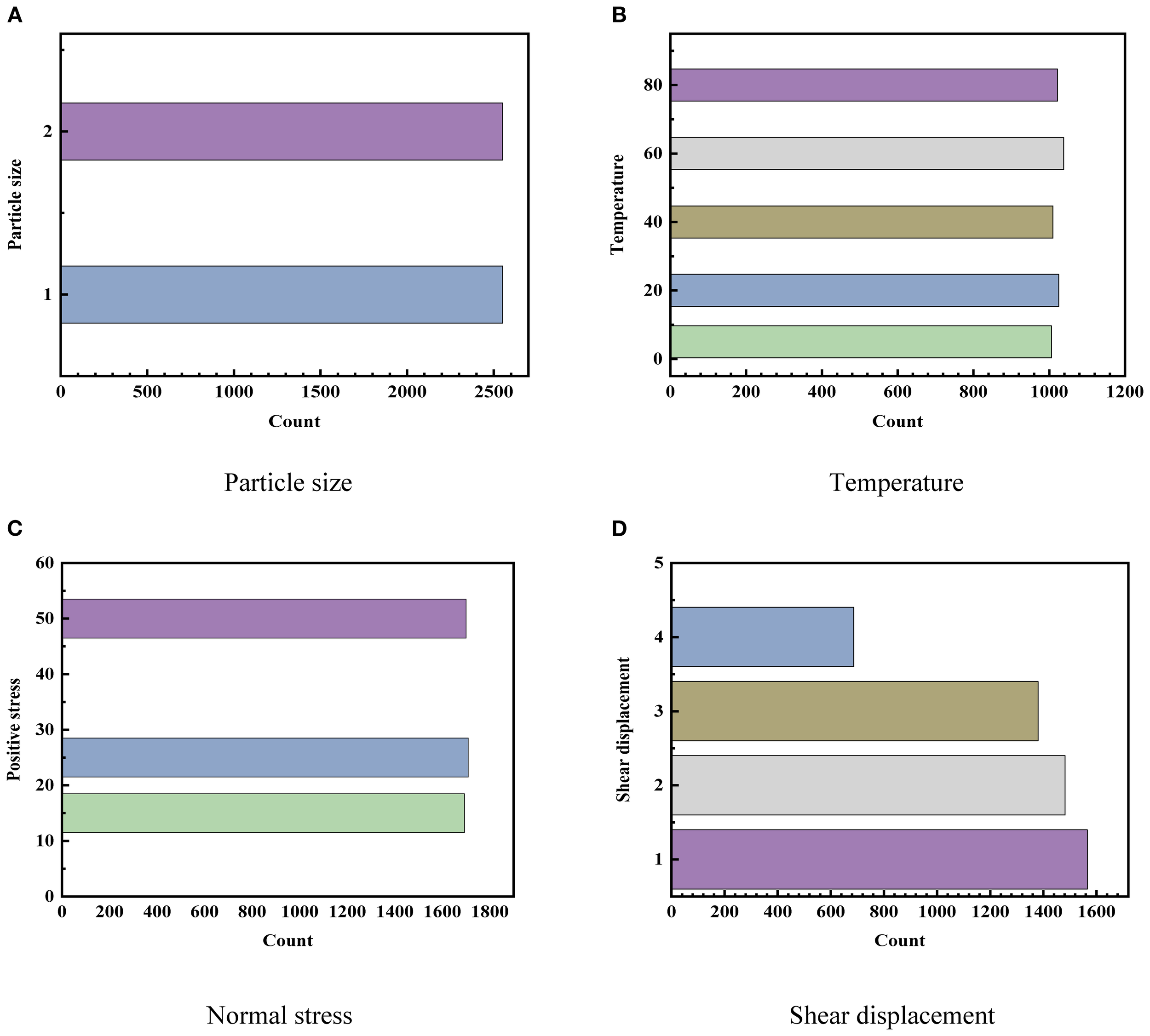
Distribution for data in the constructed database.
A database of 5102 data sets was built, which mainly included four input parameters: normal stress, temperature, particle size, and shear displacement. The dataset is split into a training set and a test set to assess the model generalization ability. The training set is utilized for model learning, while the test set serves to assess its final performance. A reasonable split of 80% for training and 20% for testing allows for a more accurate evaluation of the model generalization and practical performance.
4.2 Machine learning predicting performance
The evaluation results of machine learning model predictions using the 5102 training and testing data are depicted in Figures 7–11.
Figure 7
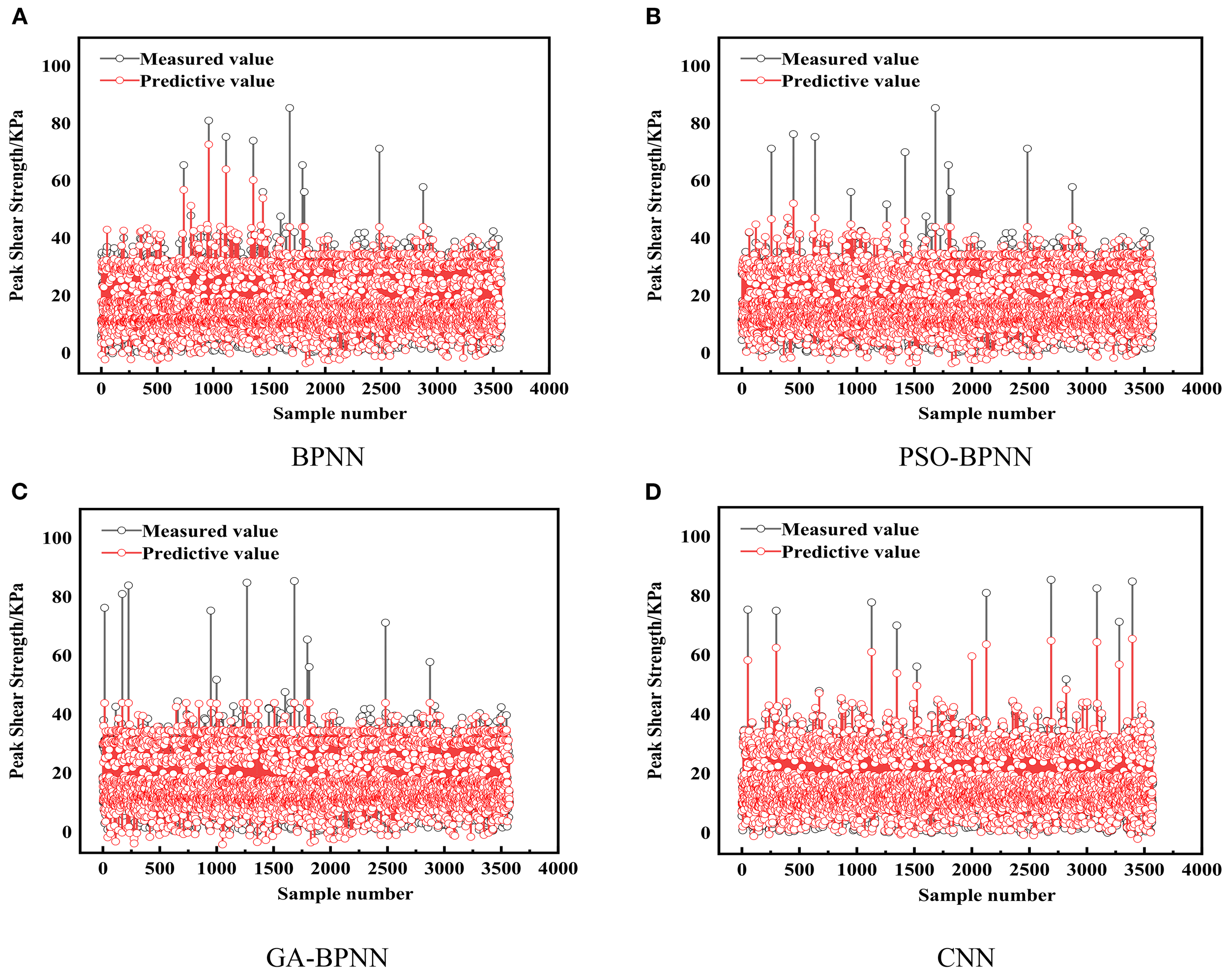
Prediction results of training set on test data.
Figure 8
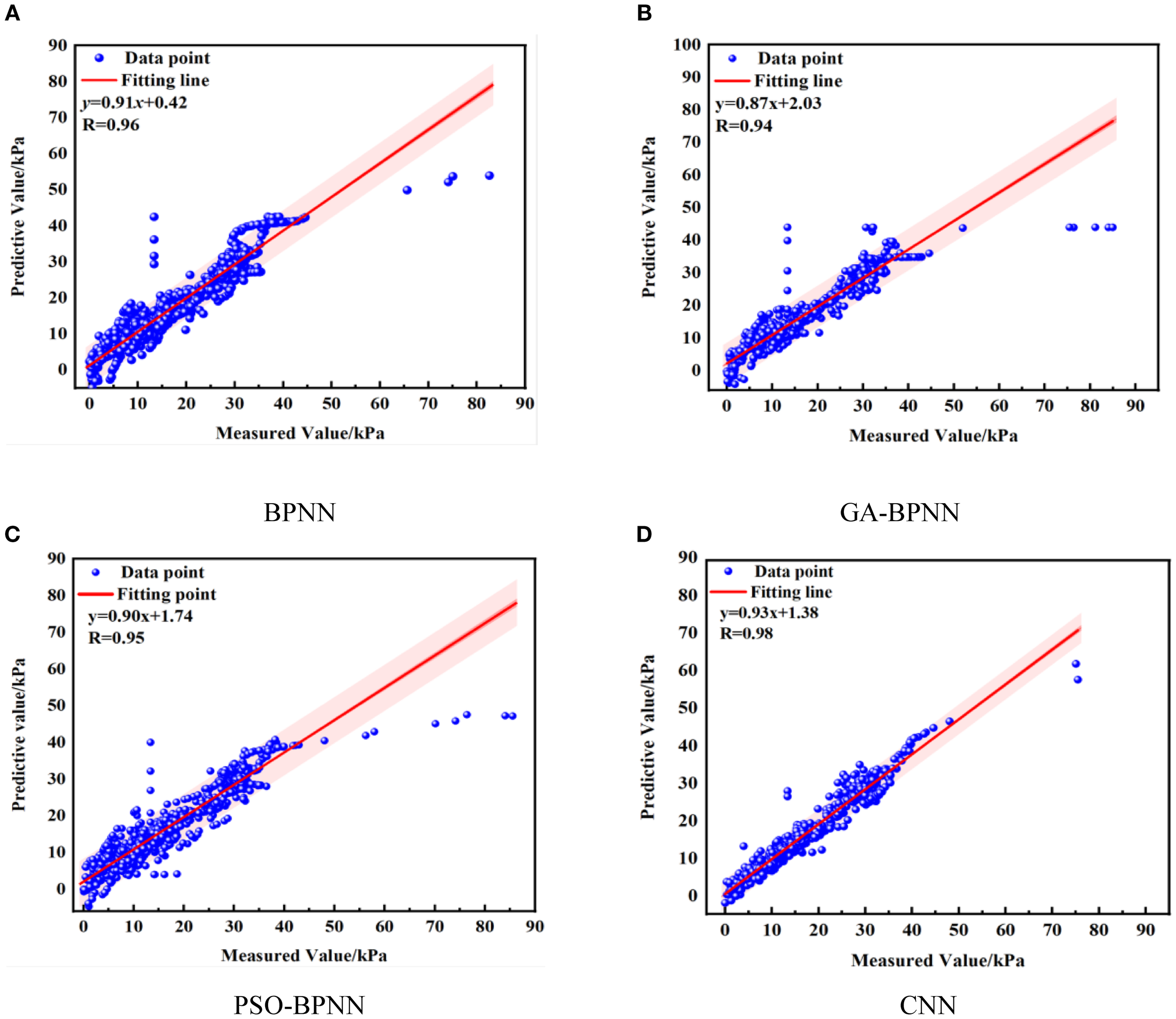
The R value of the training dataset.
Figure 9
Prediction results of test set on test data.
Figure 10
R value of the test data set.
Figure 11
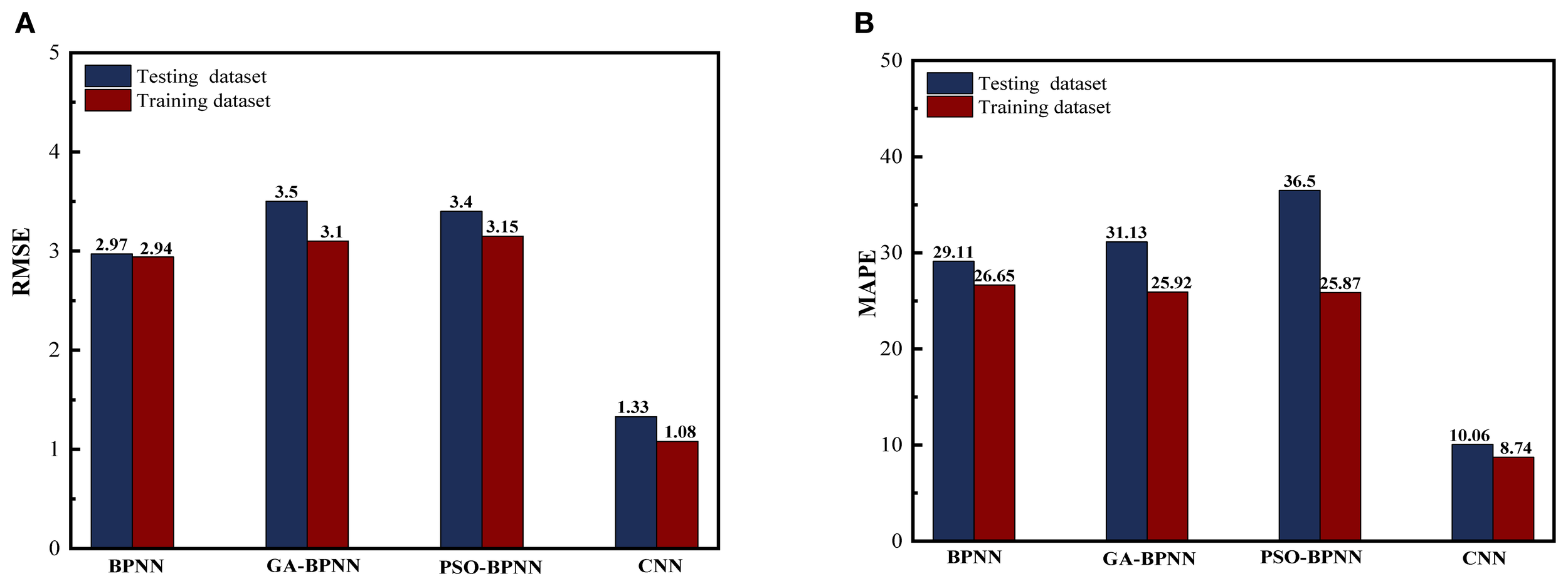
The values of the models: (A) RMSE; (B) MAPE.
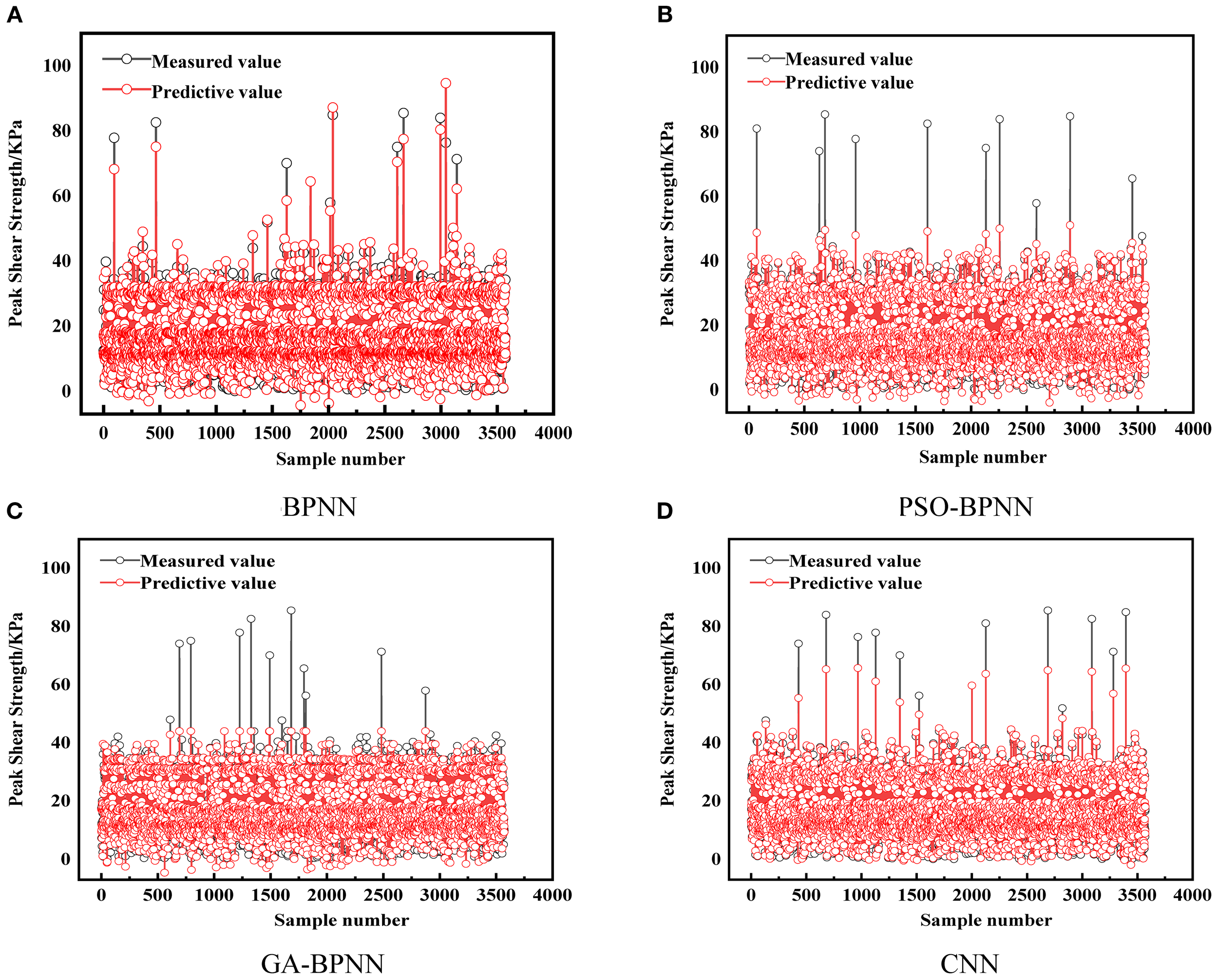
Figure 7 presents the predictions of BPNN, GA-BPNN, PSO-BPNN, and CNN on the training set. The overall trend shows that the predicted values (red solid line) and the true values (black hollow circles) of all models are consistent. Such consistency indicates that the models can fit the training data better and reflect the nonlinear relationship between the input features and the target output. In terms of error performance, there are significant differences between the different models. Among them, the prediction results of the CNN model (Figure 7D) show the smallest deviation from the true value and indicate strong fitting ability. In contrast, BPNN (Figure 7A) has a large prediction error on some samples with higher peaks, which suggests that its network structure is shallow and fails to capture the complex patterns of the data adequately. PSO-BPNN (Figure 7B) and GA-BPNN (Figure 7C) improve the performance of traditional BPNN through optimization algorithms, and the matching degree with the true value is improved, but there are still slight overfitting phenomena on some samples. In general, Figure 7 shows that the CNN model outperforms other models on the training set, with stronger learning and generalization abilities.
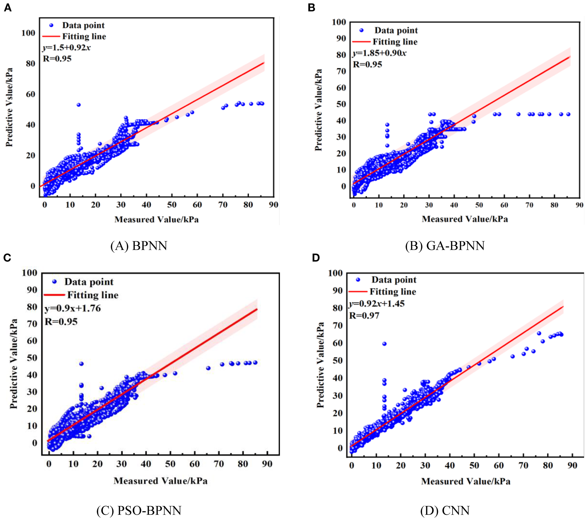
Figure 8 shows the fitting effect of each model to further evaluate the matching of the training data. CNN performs the best in the fitting graph, with the highest agreement between the fitted curve and the true value, and its R value is 0.97, which indicates that CNN can efficiently capture the patterns in the training data and fit them accurately. In contrast, the fitting effect of BPNN (Figure 8A) is poor, especially in the region with high peak values. There is a noticeable mismatch between the predicted curve and actual observations, with the R value reflecting a weak model correlation. It shows that the network depth of BPNN has some deficiencies in coping with the complex nonlinear features in the data (Xiao et al., 2024). It cannot effectively learn the complex patterns in the data. GA-BPNN and PSO-BPNN improve the fitting effect by optimizing the algorithms, but some data points are still overfitting.
As shown in Figures 9, 10, and 11, the CNN model consistently outperforms the other three machine learning models when evaluated using the test data set. Specifically, the CNN model has the highest prediction accuracy with the lowest RMSE values of 1.33 and 1.08 for the test and training sets, respectively. The lowest MAPE values of 10.06% and 8.74% for the test and training sets, respectively. In terms of the correlation coefficient, the R value of the test set for the CNN model is 0.98, close to 1, which shows a very high correlation between the predictions and the measurements. In contrast, although the prediction accuracy of the BPNN model has been improved after GA optimization, there is still a gap between the BPNN model and the CNN model. The RMSE of GA-BPNN in the test set and training set are 3.5 and 3.1, MAPE is 31.13% and 25.92%, and the R value is 0.94, which shows the limitation of GA-BPNN in capturing data regularity. The PSO-BPNN model performs relatively poorly, with larger prediction errors and more dispersed scatter distributions. Such results suggest that particle swarm optimization fails to effectively improve the prediction performance of BPNN. The RMSE of PSO-BPNN in the test set and training set is 3.4 and 3.15, respectively, and the MAPE is 36.5% and 25.87%, with an R value of 0.95. The BPNN model has the lowest prediction accuracy, with RMSE of 2.97 and 2.94 in the test set and training set, respectively, MAPE of 29.11% and 26.65%, respectively, and R value of 0.96. The results show that the data points are significantly deviated from the fitted line, which fails to capture the data patterns effectively. Due to its relatively simple model structure, it leads to insufficient ability to characterize complex data features.
Overall, the CNN model outperforms GA-BPNN, PSO-BPNN, and BPNN in evaluating both the training and test sets. Specifically, the CNN model is able to make predictions with higher accuracy and efficiency, and demonstrates the best fitting ability and prediction reliability on the test dataset. Notably, the CNN model has significantly higher prediction accuracy than the other models under the same optimization algorithm.
4.3 Sensitivity analysis
Using Grason’s algorithm, the impact of each input parameter on the interface shear strength between the marine sand and polymer layer is systematically analyzed. The relative importance of each input variable to the output variable is determined by analyzing the magnitude of the weights of each connection in the neural network. The degree of influence of the input variable xi on the output yi is calculated as follows (Equation 4):
N is the number of input neurons, L is the number of implied neurons, M is the number of output neurons, w ij is the connection weights between input neurons and implied neurons, and v jk is the connection weights between implied neurons and output neurons.
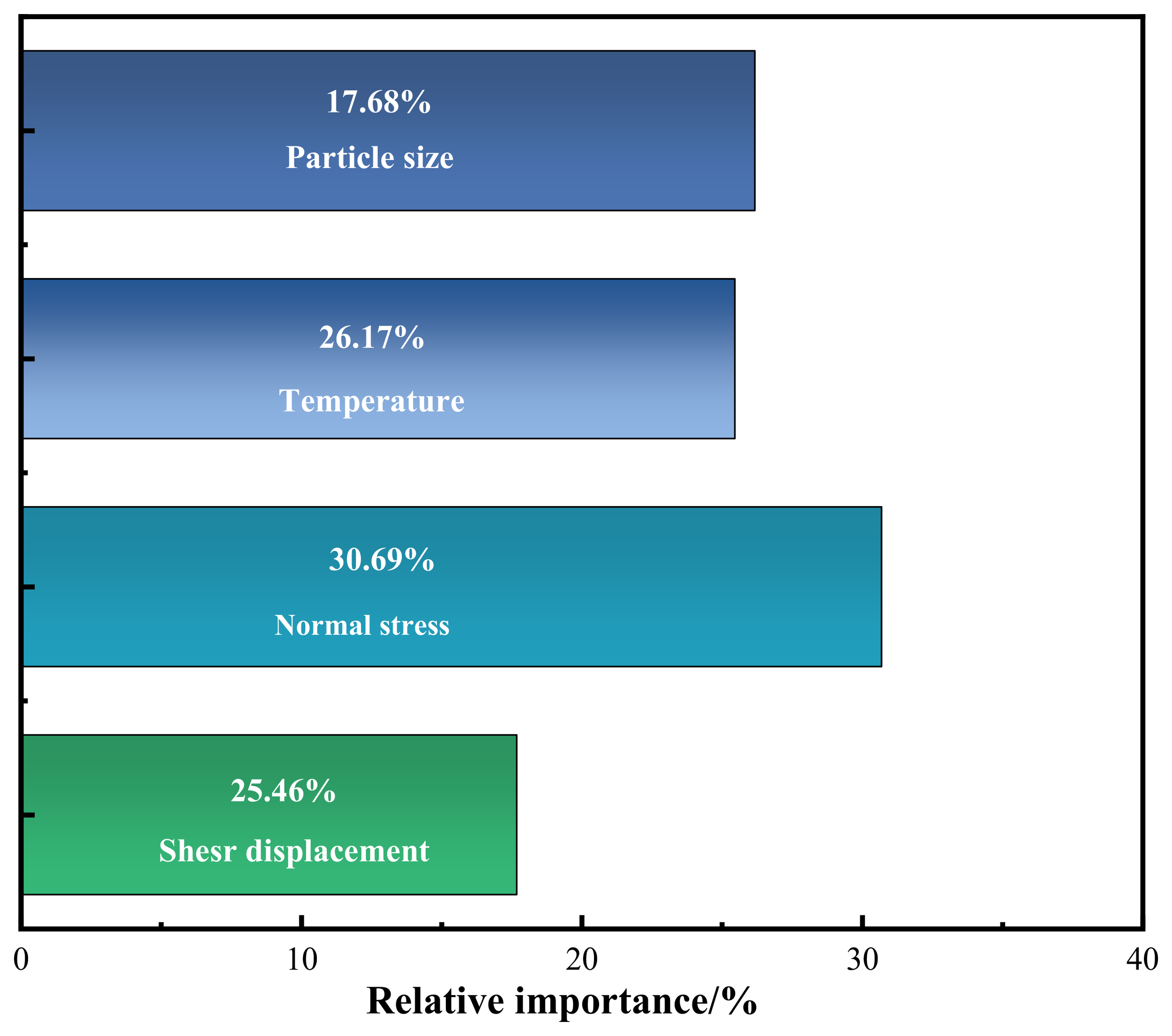
As shown in Figure 12, normal stress has the greatest influence on the MSPLI, with a relative importance of 30.69%, followed by shear displacement and temperature, with proportions of 26.17% and 25.46%, respectively. In contrast, the effect of particle size on the shear strength of MSPLI is 17.68%.
Figure 12
Relative importance of input variables.
The sensitivity analysis shows that normal stress has the greatest effect on the shear strength at this interface. The phenomenon occurs because the normal stress acts directly on the contact surface between marine sand and the polymer layer. The application of greater normal stress intensifies the contact pressure between MSPLI, which leads to stronger interfacial bonding and improved shear strength (Fan et al., 2025). However, although the relative importance of normal stress is ranked first, the extent of its influence is not dominant. Temperature ranks second in terms of its influence on the shear strength at the MSPLI. It is shown that temperature significantly affects the shear strength of the MSPLI, which highlights the critical role of considering temperature conditions when evaluating interfacial strength. The relative importance of particle size and shear displacement of 17.6% and 25.46%, respectively, on shear strength between MSPLI cannot be ignored. Therefore, to ensure the stability and reliability of the shear strength at the MSPLI, corresponding optimization measures are taken to determine the influence of different factors.
5 Empirical formula
In the study, it is shown that CNN performs better in predicting the shear strength at the MSPLI, but there are limitations in machine learning and deep learning in terms of generalization ability and interpretability. The CNN model used is applied to engineers and technicians who are not familiar with the model and may not provide effective practical guidance. In addition, the structure of the model is more complex because the architecture of the CNN incorporates a series of convolutional, pooling, and fully connected layers to extract and learn features. A more practical approach is to utilize the CNN model to generate empirical design charts and equations for engineers to use in real-world applications. The process of deriving the empirical equations is similar to P. Debnath’s method, which analyzes the training and prediction results of the model to generate empirical formulas that can be used as a reference for practice. Based on the statistical analysis of the input parameters, including temperature (T), particle size (P), normal stress (N), and shear displacement (S), the mean and the reference values have been calculated, as shown in Table 6.
Table 6
| Statistical index | Normal stress (Kpa) | Temperature (°C) | Particle size (mm) | Shear displacement (mm) |
|---|---|---|---|---|
| Mean | 30.01176 | 41.15543 | 1 | 19.18778 |
| Reference | 30 | 41 | 1 | 19 |
Reference values for different input parameters.
An empirical model was developed by considering the linear relationship between the shear strength and each parameter temperature (T), particle size (P), normal stress (N), and shear displacement (S). As shown in Figure 13, the final empirical equations for shear strength prediction using the CNN model is given by Equation 5:
Figure 13
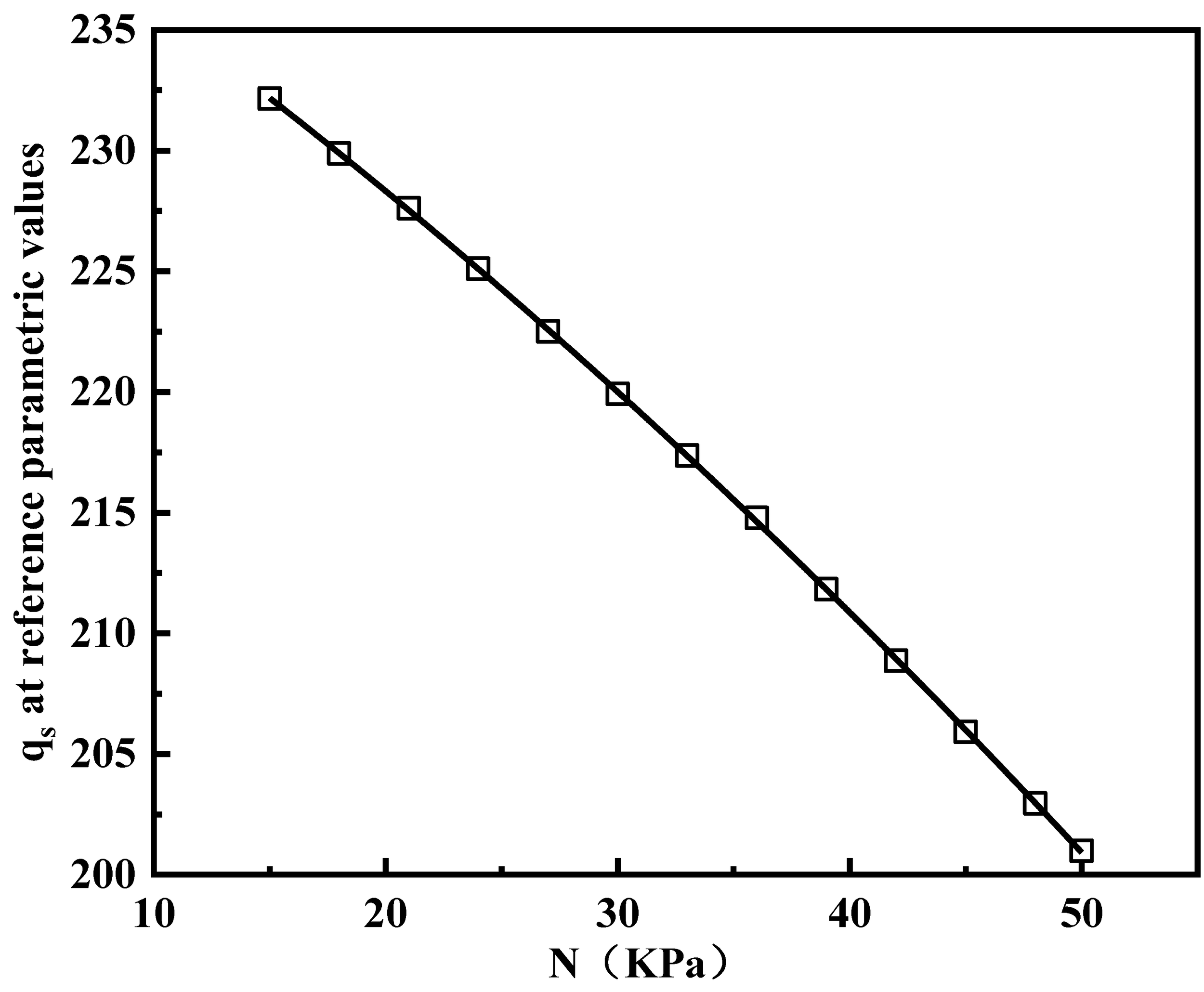
The variation of qs predicted by CNN with reference parameter N.
As can be seen from Figure 12, the most sensitive parameter is the positive stress, and to take into account the effect of other parameters, the empirical equation for shear strength (SS) prediction is given by Equation 6:
Where I chart is the s value obtained by CNN simulation from Figure 13; F is the correction function, which is introduced to consider the effect of the other four parameters on the SS prediction. The modified function F can be written as follows (Equation 7).
Using P. Debnath’s method (Debnath and Dey, 2018), the correction factor is obtained as follows (Equations 8–10):
is the correction factor for temperature, is the correction factor for particle size, and is the correction factor for shear displacement.
6 Experimental verification
Empirical equations are used to estimate the MSPLI under varying temperature scenarios, and the results are compared with experimental findings to evaluate the performance of the deep learning and empirical models. According to the data in Table 7, 30 sets of tests are selected. According to the experimental conditions and requirements, formula (4) is used to estimate the shear strength of the MSPLI with different particle size grading under different conditions. The predicted shear strength is compared with the previously studied shear strength, as shown in Figure 14.
Table 7
| Particle size (mm) | Temperature (°C) | Normal stress (KPa) | Shear displacement (S) |
|---|---|---|---|
| S1 | 5 | 15 | 2.3176 |
| 5 | 25 | 1.0466 | |
| 5 | 50 | 1.9407 | |
| S2 | 5 | 15 | 1.3208 |
| 5 | 25 | 3.6135 | |
| 5 | 50 | 2.1369 | |
| S1 | 20 | 15 | 4.66 |
| 20 | 25 | 3.321 | |
| 20 | 50 | 3.557 | |
| S2 | 20 | 15 | 4.383 |
| 20 | 25 | 2.691 | |
| 20 | 50 | 8.511 | |
| S1 | 40 | 15 | 9.19 |
| 40 | 25 | 9.246 | |
| 40 | 50 | 11.096 | |
| S2 | 40 | 15 | 8.021 |
| 40 | 25 | 8.454 | |
| 40 | 50 | 4.61 | |
| S1 | 60 | 15 | 51.808 |
| 60 | 25 | 68.184 | |
| 60 | 50 | 13.557 | |
| S2 | 60 | 15 | 11.495 |
| 60 | 25 | 7.383 | |
| 60 | 50 | 7.099 | |
| S1 | 80 | 15 | 13.9745 |
| 80 | 25 | 13.5072 | |
| 80 | 50 | 10.9154 | |
| S2 | 80 | 15 | 50.415 |
| 80 | 25 | 16.124 | |
| 80 | 50 | 15.4013 |
30 sets of data selected for the experiment.
To further validate the applicability of the empirical approach, the predictive performance under different temperature conditions is examined. As shown in Figure 14, the use of empirical formulas to predict the effect of marine sand and polymer layer interfacial response under different temperature conditions is more effective. The results showed an RMSE of 0.68, a MAPE of 3.87%, and an R²of 0.99. It is concluded that the developed empirical formulation shows good accuracy and reliability in predicting the response of the MSPLI. It can efficiently capture the response variations under different temperature conditions, and those who do not know deep learning are provided with an easy and efficient tool. Used to quickly estimate and predict the performance of MSPLI, it reduces the reliance on complex models and can provide an important reference in engineering design and decision-making.
Figure 14
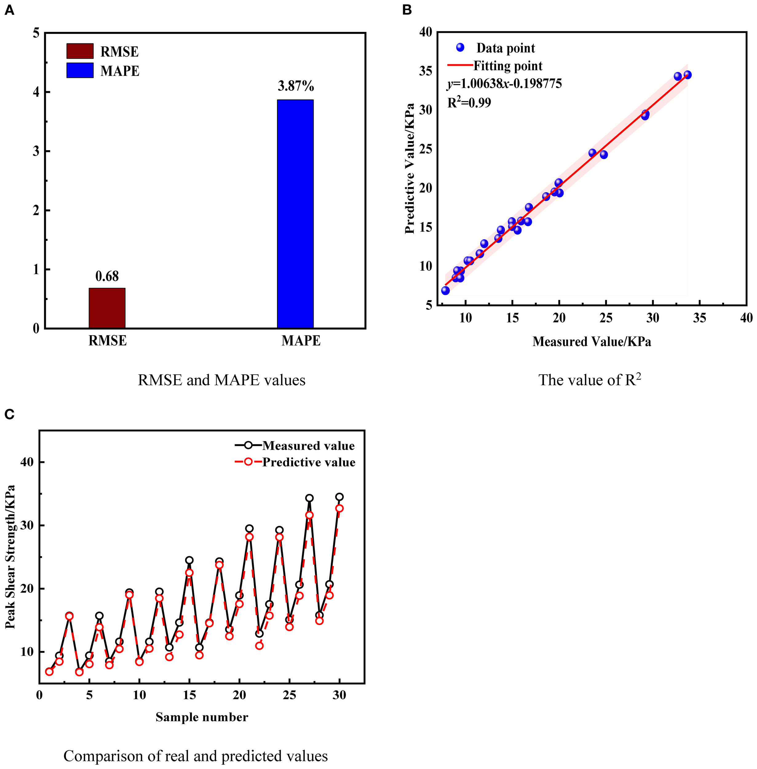
Performance evaluation of marine sand and polymer layer interface shear strength prediction based on empirical equations.
7 Conclusions
The study involves conducting experimental tests to evaluate the shear strength at the marine sand and polymer layer interface (MSPLI) under various temperatures. The results are used to build a database. Based on this, a CNN model using deep learning is established to predict the shear strength at the MSPLI. The model integrates key input parameters that affect interfacial shear strength, including shear displacement, particle size, normal stress, and temperature. To validate the CNN model performance, three conventional machine learning models(BPNN, GA-BPNN, and PSO-BPNN)are also constructed. Their prediction performance is analyzed and compared. In addition, sensitivity analysis is conducted to evaluate the influence of each input variable on the interfacial shear strength. Ultimately, based on the analyzed results, an empirical formula is proposed. This formula is intended for direct application in practical engineering by engineers and technicians who lack expertise in machine learning. The main research results are as follows:
-
The shear strength at the MSPLI decreases with the increase in temperature. Because the high temperature softens the polymer layer and weakens the interface friction. The finding highlights the importance of monitoring and optimizing the properties of polymer layers at high temperatures to ensure the long-term stability of engineering structures.
-
The deep learning model based on convolutional neural network (CNN) performs well in predicting the shear strength at the MSPLI, with RMSE of 1.08 and 1.33 for the training and test sets, respectively, which is significantly better than that of traditional machine learning models (BPNN, GA-BPNN, and PSO-BPNN). The model not only captures complex nonlinear relationships but also demonstrates higher robustness and prediction accuracy when dealing with multivariate inputs.
-
The sensitivity analysis shows that the normal stress has the greatest influence on the shear strength at the MSPLI, which is followed by temperature, shear displacement, and grain size. The result provides a scientific basis for prioritizing and optimizing key parameters in engineering design, which helps to improve the efficiency and effectiveness of engineering design.
-
The proposed empirical formula based on experimental data and modeling results provides a simple and efficient prediction tool for engineers and technicians. The formula reduces the dependence on complex models and can provide an important reference in engineering design and decision-making. Especially in the case of limited resources or insufficient computational capacity, and it has important practical application value.
Overall, accurate prediction of the shear strength between the MSPLI is challenging because it is affected by multiple complex nonlinear factors. However, the CNN deep learning model proposed in the study successfully addresses these challenges and can effectively predict the effects of key factors such as temperature, normal stress, particle size, and shear displacement on shear strength (Wang et al., 2024). Compared with traditional methods, the CNN model demonstrates superior predictive accuracy, robustness, and ability to handle complex multivariate interactions, emphasizing the necessity and practical advantage of AI approaches in engineering applications. The model provides strong support for the engineering application and design of shear strength at the MSPLI, especially in scenarios with limited computational resources. The empirical equations constructed based on the experimental results can provide engineers and technicians with a convenient and efficient prediction tool (Zheng et al., 2024c). Future studies should further consider other properties of sand particles, such as particle shape and surface roughness, and extend the existing database to enhance the model generalization ability (Zheng et al., 2024b). In addition, more experimental studies under different working conditions are recommended to further validate and optimize the performance of the model. These improvements enable the model to perform more stably and reliably in different engineering scenarios, thereby providing more accurate predictions and stronger technical support for practical engineering applications.
Statements
Data availability statement
The original contributions presented in the study are included in the article/supplementary material. Further inquiries can be directed to the corresponding authors.
Author contributions
ZC: Resources, Writing – original draft, Writing – review & editing, Supervision, Data curation, Methodology, Conceptualization. YL: Methodology, Data curation, Software, Writing – review & editing, Validation, Conceptualization, Visualization, Formal Analysis, Writing – original draft. DJ: Writing – review & editing, Supervision, Writing – original draft, Data curation, Formal Analysis. HD: Writing – review & editing, Conceptualization, Supervision, Project administration, Writing – original draft, Formal Analysis. WY: Project administration, Investigation, Writing – review & editing, Writing – original draft, Software. XF: Investigation, Writing – review & editing, Software, Writing – original draft, Methodology. JL: Validation, Writing – review & editing, Investigation, Writing – original draft, Formal Analysis. PC: Conceptualization, Supervision, Writing – review & editing, Writing – original draft. ZW: Methodology, Validation, Investigation, Writing – review & editing, Writing – original draft, Conceptualization.
Funding
The author(s) declare financial support was received for the research and/or publication of this article. The authors acknowledge the consistent support of the following funding sources: National Natural Science Foundation of China (No. 52471290, No. 52301327); China Postdoctoral Science Foundation (No. 2024T170217, No. 2023M730929); Failure Mechanics and Engineering Disaster Prevention, Key Lab of Sichuan Province (No. FMEDP202209); Shanghai Sailing Program (No. 22YF1415800, No. 23YF1416100); Shanghai Natural Science Foundation (No. 23ZR1426200, No. 24ZR1427900); Shanghai Soft Science Key Project (No. 23692119700); Key Laboratory of Ministry of Education for Coastal Disaster and Protection, Hohai University (No. 202302); Key Laboratory of Estuarine & Coastal Engineering, Ministry of Transport (No. KLECE220302); and Shanghai Frontiers Science Center of “Full Penetration” Far-Reaching Offshore Ocean Energy and Power.
Conflict of interest
Author DJ was employed by the company Power China Kunming Engineering Corporation Limited and author XF was employed by the company CCCC-FHDI Engineering Co., Ltd.
The remaining authors declare that the research was conducted in the absence of any commercial or financial relationships that could be construed as a potential conflict of interest.
Generative AI statement
The author(s) declare that no Generative AI was used in the creation of this manuscript.
Any alternative text (alt text) provided alongside figures in this article has been generated by Frontiers with the support of artificial intelligence and reasonable efforts have been made to ensure accuracy, including review by the authors wherever possible. If you identify any issues, please contact us.
Publisher’s note
All claims expressed in this article are solely those of the authors and do not necessarily represent those of their affiliated organizations, or those of the publisher, the editors and the reviewers. Any product that may be evaluated in this article, or claim that may be made by its manufacturer, is not guaranteed or endorsed by the publisher.
References
1
Akpinar M. V. Benson C. H. (2005). Effect of temperature on shear strength of two geomembrane–geotextile interfaces. Geotext Geomembranes23, 443–453. doi: 10.1016/j.geotexmem.2005.02.004
2
Bilgin Ö. Stewart H. E. (2006). “ Effect of temperature on surface hardness and soil interface shear resistance of geosynthetics,” in Proc., 8th Int. Conf. on Geosynthetics, (Rotterdam, Netherlands: Millpress) Vol. 1. 251–254.
3
Chao Z. et al . (2024e). Permeability and porosity of light-weight concrete with plastic waste aggregate: Experimental study and machine learning modelling. Constr. Build Mater.411, 134465. doi: 10.1016/j.conbuildmat.2023.134465
4
Chao Z. Fowmes G. Mousa A. Zhou J. Zhao Z. Zheng J. et al . (2024a). A new large-scale shear apparatus for testing geosynthetics-soil interfaces incorporating thermal condition. Geotext Geomembranes52, 999–1010. doi: 10.1016/j.geotexmem.2024.06.002
5
Chao Z. Li Z. Dong Y. Shi D. Zheng J. (2024b). Estimating compressive strength of coral sand aggregate concrete in marine environment by combining physical experiments and machine learning-based techniques. Ocean Eng.308, 118320. doi: 10.1016/j.oceaneng.2024.118320
6
Chao Z. Liu H. Wang H. Dong Y. Shi D. Zheng J. (2024c). The interface mechanical properties between polymer layer and marine sand with different particle sizes under the effect of temperature: Laboratory tests and artificial intelligence modelling. Ocean Eng.312, 119255. doi: 10.1016/j.oceaneng.2024.119255
7
Chao Z. Shi D. Fowmes G. Xu X. Yue W. Cui P. et al . (2023a). Artificial intelligence algorithms for predicting peak shear strength of clayey soil-geomembrane interfaces and experimental validation. Geotext Geomembranes51, 179–198. doi: 10.1016/j.geotexmem.2022.10.007
8
Chao Z. Shi D. Zheng J. (2024d). Experimental research on temperature–Dependent dynamic interface interaction between marine coral sand and polymer layer. Ocean Eng.297, 117100. doi: 10.1016/j.oceaneng.2024.117100
9
Chao Z. Wang H. Hu H. Ding T. Zhang Y. (2023b). Predicting the temperature-dependent long-term creep mechanical response of silica sand-textured geomembrane interfaces based on physical tests and machine learning techniques. Materials16, 6144. doi: 10.3390/ma16186144
10
Chao Z. Wang M. Sun Y. Xu X. Yue W. Yang C. et al . (2022). Predicting stress-dependent gas permeability of cement mortar with different relative moisture contents based on hybrid ensemble artificial intelligence algorithms. Constr. Build Mater.348, 128660. doi: 10.1109/GUCON.2018.8675097
11
Chao Z. Wang H. Zheng J. Shi D. Li C. Ding G. et al . (2024f). Temperature-dependent post-cyclic mechanical characteristics of interfaces between geogrid and marine reef sand: experimental research and machine learning modeling. J. Mar. Sci. Eng.12, 1262. doi: 10.3390/jmse12081262
12
Chao Z. Yang C. Zhang W. Zhang Y. Zhou J. (2023c). Predicting the gas permeability of sustainable cement mortar containing internal cracks by combining physical experiments and hybrid ensemble artificial intelligence algorithms. Materials16, 5330. doi: 10.3390/ma16155330
13
Chao Z. Zhao H. Liu H. Cui P. Shi D. Lin H. et al . (2024g). The temperature-dependent monotonic mechanical characteristics of marine sand–geomembrane interfaces. J. Mar. Sci. Eng.12, 1262. doi: 10.3390/jmse12122193
14
Chao Z. Zhou J. Shi D. Zheng J. (2025). Particle size effect on the mechanical behavior of coral sand–geogrid interfaces. Geosynth. Int.32, 1–17. doi: 10.1680/jgein.24.00143
15
Chauhan N. K. Singh K. (2018). A review on conventional machine learning vs deep learning. IEEE2018, 347–352. doi: 10.1109/GUCON.2018.8675097
16
Chen D. Li G. He P. Zhang H. Sheng J. Wang M. (2025). Investigating the shear characteristics of geomembrane–sand interfaces under freezing conditions. Designs9, 9. doi: 10.3390/designs9010009
17
Cheng Z. Wang J. Xiong W. (2023). A machine learning-based strategy for experimentally estimating force chains of granular materials using X-ray micro-tomography. Géotechnique74, 1291–1303. doi: 10.1680/jgeot.21.00281
18
Cui J. Jin Y. Jing Y. Lu Y. (2024). Elastoplastic solution of cylindrical cavity expansion in unsaturated offshore island soil considering anisotropy. J. Mar. Sci. Eng.12, 308. doi: 10.3390/jmse12020308
19
Debnath P. Dey A. K. (2018). Prediction of bearing capacity of geogrid-reinforced stone columns using support vector regression. Int. J. Geomech.18, 04017147. doi: 10.1061/(ASCE)GM.1943-5622.0001067
20
Ding S. Li S. Kong S. Li Q. Yang T. Nie Z. et al . (2024). Changing of mechanical property and bearing capacity of strongly chlorine saline soil under freeze-thaw cycles. Sci. Rep-UK.14, 6203. doi: 10.1038/s441598-024-56822-8
21
Divya P. V. Viswanadham B. V. S. Gourc J. P. (2012). Influence of geomembrane on the deformation behaviour of clay-based landfill covers. Geotext Geomembranes34, 158–171. doi: 10.1016/j.geotexmem.2012.06.002
22
Dong Y. Wang D. Randolph M. F. (2017). Investigation of impact forces on pipeline by submarine landslide using material point method. Ocean Eng.146, 21–28. doi: 10.1016/j.oceaneng.2017.09.008
23
El-Saadony M. T. Saad A. M. El-Wafai N. A. Abou-Aly H. E. Salem H. M. Soliman S. M. et al . (2023). Hazardous wastes and management strategies of landfill leachates: A comprehensive review. Environ. Technol. Inno.31, 103150. doi: 10.1016/j.eti.2023.103150
24
Fan L. Cui L. Zhu Z. Sheng Q. Zheng J. Dong Y. (2025). Elaborate numerical analysis and new fibre Bragg grating monitoring methods for the ground pressure in shallow large-diameter shield tunnels: a case study of the yellow crane tower tunnel project. B. Eng. Geol. Environ.84, 1–19. doi: 10.1007/s10064-025-04088-3
25
Fan N. Jiang J. Nian T. Dong Y. Guo L. Fu C. et al . (2023). Impact action of submarine slides on pipelines: A review of the state-of-the-art since 2008. Ocean Eng.286, 115532. doi: 10.1016/j.oceaneng.2023.115532
26
Gao R. Ye J. (2023). Mechanical behaviors of coral sand and relationship between particle breakage and plastic work. Eng. Geol.316, 107063. doi: 10.1016/j.enggeo.2023.107063
27
Gao R. Ye J. (2024). A novel relationship between elastic modulus and void ratio associated with principal stress for coral calcareous sand. J. Rock. Mech. Geotech.16, 1033–1048. doi: 10.1016/j.jrmge.2023.07.011
28
Gong J. Wang L. Xu J. Li Y. Tang Z. (2025a). Study on the surf-riding and broaching of trimaran with different control schemes. Ocean Eng.324, 120644. doi: 10.1016/j.oceaneng.2025.120644
29
Gong J. Xu J. Xu L. Hong Z. (2025b). Enhancing motion forecasting of ship sailing in irregular waves based on optimized LSTM model and principal component of wave-height. Front. Mar. Sci.12. doi: 10.3389/fmars.2025.1497956
30
Guo R. Xiao G. Zhang C. Li Q. (2025). A study on influencing factors of port cargo throughput based on multi-scale geographically weighted regression. Front. Mar. Sci.12. doi: 10.3389/fmars.2025.1637660
31
Hajihassani M. Jahed Armaghani D. Kalatehjari R. (2018). Applications of particle swarm optimization in geotechnical engineering: a comprehensive review. Geotech. Geol. Eng.36, 705–722. doi: 10.1007/s10706-017-0356-z
32
Hamidi A. Garousi A. H. (2024). Grain size effect on the anisotropic shear behavior of sand–textured geomembrane interface. Proc. Inst. Civ. Eng-Gr.177, 310–323. doi: 10.1680/jgrim.23.0001.
33
Huang Z. Liu G. Zhang Y. Yuan Y. Xi B. Tan W. (2024). Assessing the impacts and contamination potentials of landfill leachate on adjacent groundwater systems. Sci. Total Environ.930, 172664. doi: 10.1016/j.scitotenv.2024.172664
34
Jin L. Duan J. Jin Y. Xue P. Zhou P. (2024). Prediction of HPC compressive strength based on machine learning. Sci. Rep-UK.14, 16776. doi: 10.1038/s41598-024-67850-9
35
Kamath C. N. Bukhari S. S. Dengel A. (2018). “ Comparative study between traditional machine learning and deep learning approaches for text classification,” in Proceedings of the ACM Symposium on Document Engineering. (Pittsburgh, PA, USA: ACM), 1–11. doi: 10.1145/3209280.3209526
36
Karademir T. Frost J. D. (2021). Elevated temperature effects on geotextile–geomembrane interface shear behavior. J. Geotech. Geoenviron.147, 04021148. doi: 10.1061/(ASCE)GT.1943-5606.0002698
37
Katoch S. Chauhan S. S. Kumar V. (2021). A review on genetic algorithm: past, present, and future. Multimed. Tools Appl.80, 8091–8126. doi: 10.1007/s11042-020-10139-6
38
Khan R. Latha G. M. (2025). Multi-scale behaviour of sand-geosynthetic interactions considering particle size effects. Geotext Geomembranes53, 169–187. doi: 10.1016/j.geotexmem.2024.09.008
39
Lai Y. (2019). “ A comparison of traditional machine learning and deep learning in image recognition,” in Journal of Physics: Conference Series, vol. 1314. (Bristol, United Kingdom: IOP Publishing), 012148. doi: 10.1088/1742-6596/1314/1/012148
40
Li D. Jiang Z. Tian K. Ji R. (2025). Prediction of hydraulic conductivity of sodium bentonite GCLs by machine learning approaches. Environ. Geotech.12, 154–173. doi: 10.1680/jenge.22.00181
41
Li C. Zhang M. Zhang X. (2023). Enhancing concrete creep prediction with deep learning: A soft-sorted one-dimensional cnn approach. IEEE Access. 11, 139314–139325. doi: 10.1109/ACCESS.2023.3340425
42
Li T. Zhu Z. Wu T. Ren G. Zhao G. (2024). A potential way for improving the dispersivity and mechanical properties of dispersive soil using calcined coal gangue. J. Mater. Res. Technol.29, 3049–3062. doi: 10.1016/j.jmrt.2024.01.281
43
Liang H. Shen Y. Xu J. Shen J. Xie W. C. (2025). Effects of particle sphericity on shear behaviors of uniformly graded sand: Experimental study based on 3D printing. B. Eng. Geol. Environ.84, 120. doi: 10.1007/s10064-025-04132-2
44
Lin H. Gong X. Zeng Y. Zhou C. (2024). Experimental study on the effect of temperature on HDPE geomembrane/geotextile interface shear characteristics. Geotext Geomembranes52, 396–407. doi: 10.1016/j.geotexmem.2023.12.005
45
Liu B. Wang Z. Muhodir S. H. Alanazi A. Alsubai S. Alqahtani A. (2024). Prediction of rock slope failure using multiple ML algorithms. Geomech. Eng.36, 489–509. doi: 10.12989/gae.2024.36.5.489
46
Paterakis N. G. Mocanu E. Gibescu M. Stappers B. van Alst W. (2017). “ Deep learning versus traditional machine learning methods for aggregated energy demand prediction,” in 2017 IEEE PES Innovative Smart Grid Technologies Conference Europe (ISGT-Europe). (Piscataway, New Jersey, USA: IEEE), 1–6. doi: 10.1109/ISGTEurope.2017.8260289
47
Reddy N. S. Senetakis K. He H. (2022). “ Micromechanical insights on the stiffness of sands through grain-scale tests and DEM analyses,” in Indian Geotechnical Conference ( Springer Nature Singapore, Singapore), 213–225. doi: 10.1007/978-981-97-6168-5
48
Ren P. Chen Z.-L. Li L. Gong W. Li J. (2024). Dynamic shakedown behaviors of flexible pavement overlying saturated ground under moving traffic load considering effect of pavement roughness. Comput. Geotech.168, 106134. doi: 10.1016/j.compgeo.2024.106134
49
Ren S. He K. Girshick R. Sun J. (2016). Faster R-CNN: Towards real-time object detection with region proposal networks. IEEE T Pattern Anal.39, 1137–1149. doi: 10.1109/TPAMI.2016.2577031
50
Rowe R. K. Islam M. Z. (2009). Impact of landfill liner time–temperature history on the service life of HDPE geomembranes. Waste Manage.29, 2689–2699. doi: 10.1016/j.wasman.2009.05.010
51
Sangam H. P. (2001). Performance of HDPE geomembrane liners in landfill applications.
52
Schmidhuber J. (2015). Deep learning in neural networks: An overview. Neural Netw.61, 85–117. doi: 10.1016/j.neunet.2014.09.003
53
Sevim Ö. Demir I. (2019). Physical and permeability properties of cementitious mortars having fly ash with optimized particle size distribution. Cement Concrete Comp.96, 266–273. doi: 10.1016/j.cemconcomp.2018.11.017
54
Shao W. Qin F. Shi D. Soomro M. A. (2024). Horizontal bearing characteristic and seismic fragility analysis of CFRP composite pipe piles subject to chloride corrosion. Comput. Geotech.166, 105977. doi: 10.1016/j.compgeo.2023.105977
55
Shi D. Niu J. Zhang J. Chao Z. Fowmes G. (2023). Effects of particle breakage on the mechanical characteristics of geogrid-reinforced granular soils under triaxial shear: A DEM investigation. Geomech. Energy Envir.34, 100446. doi: 10.1016/j.gete.2023.100446
56
Shi D. Xu K. Chao Z. Cui P. Experimental study on mechanical properties of triaxial geogrid reinforced marine coral sand-clay mixture based on 3d printing technology. Front. Mar. Sci. doi: 10.2139/ssrn.5270666
57
Shi D. Xu K. Yu X. Chao Z. Cui P. (2025) Strength estimation of textured polymer layer-reinforced materials in practical marine engineering based on physical experiments and artificial intelligence modelling. Front. Mar. Sci.12. doi: 10.3389/fmars.2025.1653741
58
Shu Z. Gan X. Xie J. Dai Z. Li Z. (2025). A macroscopic peridynamic approach for glulam embedment failure simulations. J. Build Eng.106, 112587. doi: 10.1016/j.jobe.2025.112587
59
Singh R. K. Datta M. Nema A. K. (2009). A new system for groundwater contamination hazard rating of landfills. J. Environ. Manage.91, 344–357. doi: 10.1016/j.jenvman.2009.09.003
60
Song S. Wang P. Yin Z. Cheng Y. (2024). Micromechanical modeling of hollow cylinder torsional shear test on sand using discrete element method. J. Rock. Mech. Geotech.16, 5193–5208. doi: 10.1016/j.jrmge.2024.02.010
61
Sun S. Cao Z. Zhu H. Zhao J. (2019). A survey of optimization methods from a machine learning perspective. IEEE T Cybernet.50, 3668–3681. doi: 10.1109/TCYB.2019.2950779
62
Wang T. Xiao G. Li Q. Biancardo S. A. (2025). The impact of the 21st-Century Maritime Silk Road on sulfur dioxide emissions in Chinese ports: based on the difference-in-difference model. Front. Mar. Sci.12. doi: 10.3389/fmars.2025.1608803
63
Wang F. Zhai W. Man J. Huang H. (2024). A hybrid cohesive phase-field numerical method for the stability analysis of rock slopes with discontinuities. Can. Geotech. J. doi: 10.1139/cgj-2024-0382
64
Wang F. Zhang D. Huang H. Huang Q. (2023). A phase-field-based multi-physics coupling numerical method and its application in soil–water inrush accident of shield tunnel. Tunn Undergr. Sp. Tech.140, 105233. doi: 10.1016/j.tust.2023.105233
65
Xiao G. Amamoo-Otoo C. Wang T. Li Q. Biancardo S. A. (2025). Evaluating the impact of ECA policy on sulfur emissions from the five busiest ports in America based on difference in difference model. Front. Mar. Sci.12. doi: 10.3389/fmars.2025.1609261
66
Xiao M. Luo R. Chen Y. Ge X. (2023). Prediction model of asphalt pavement functional and structural performance using PSO-BPNN algorithm. Constr. Build Mater.407, 133534. doi: 10.1016/j.conbuildmat.2023.133534
67
Xiao G. Wang Y. Wu R. Li J. Cai Z. (2024). Sustainable maritime transport: A review of intelligent shipping technology and green port construction applications. J. Mar. Sci. Eng.12, 1728. doi: 10.3390/jmse12101728
68
Xiao G. Xu L. (2024). Challenges and opportunities of maritime transport in the post-epidemic era. J. Mar. Sci. Eng.12, 1685. doi: 10.3390/jmse12091685
69
Xu J. Gong J. Li Y. Fu Z. Wang L. (2024). Surf-riding and broaching prediction of ship sailing in regular waves by LSTM based on the data of ship motion and encounter wave. Ocean Eng.297, 117010. doi: 10.1016/j.oceaneng.2024.117010
70
Yang J. Wan H. Shang Z. (2025). Enhanced hybrid CNN and transformer network for remote sensing image change detection. Sci. Rep-UK.15, 10161. doi: 10.1038/s41598-025-94544-7
71
Ye J. Gao R. (2024). Isotropic compression and triaxial shear characteristics of coral sand under high confining pressure and related particle breakage. Geotechnique75, 1218–1234. doi: 10.1680/jgeot.24.01260
72
Ye J. Zhang Z. Shan J. (2019). Statistics-based method for determination of drag coefficient for nonlinear porous flow in calcareous sand soil. B. Eng. Geol. Environ.78, 3663–3670. doi: 10.1007/s10064-018-1330-6
73
Yin Q. Wu J. Zhu C. He M. Meng Q. Jing H. (2021). Shear mechanical responses of sandstone exposed to high temperature under constant normal stiffness boundary conditions. Geomech. Geophys. Geo.7, 1–17. doi: 10.1007/S40948-021-00234-9
74
Zhang W. Li H. Shi D. Shen Z. Zhao S. Guo C. (2023a). Determination of safety monitoring indices for roller-compacted concrete dams considering seepage–stress coupling effects. Mathematics-Basel11, 3224. doi: 10.3390/math11143224
75
Zhang J. Liu B. Zhu Z. (2024). Investigation on shear strength properties of water-bearingconcrete-rock interface based on convolutional neural network recognition method. Constr. Build Mater.440, 137349. doi: 10.1016/j.conbuildmat.2024.137349
76
Zhang Y. Zhang Z. Zheng J. Zheng Y. Zhang J. Liu Z. et al . (2023b). Research of the array spacing effect on wake interaction of tidal stream turbines. Ocean Eng.276, 114227. doi: 10.1016/j.oceaneng.2023.114227
77
Zhao S. Zhang J. Feng S. (2023b). The era of low-permeability sites remediation and corresponding technologies: A review. Chemosphere313, 137264. doi: 10.1016/j.chemosphere.2022.137264
78
Zhao G. Zhu Z. Ren G. Wu T. Ju P. Ding S. et al . (2023a). Utilization of recycled concrete powder in modification of the dispersive soil: A potential way to improve the engineering properties. Constr. Build Mater.389, 131626. doi: 10.1016/j.conbuildmat.2023.131626
79
Zheng Z. Deng B. Li S. Zheng H. (2024a). Disturbance mechanical behaviors and anisotropic fracturing mechanisms of rock under novel three-stage true triaxial static-dynamic coupling loading. Rock. Mech. Rock. Eng.57, 2445–2468. doi: 10.1007/s00603-023-03696-3
80
Zheng Z. Deng B. Liu H. Wang W. Huang S. Li S. (2024b). Microdynamic mechanical properties and fracture evolution mechanism of monzogabbro with a true triaxial multilevel disturbance method. Int. J. Min. Sci. Tech.34, 385–411. doi: 10.1016/j.ijmst.2024.01.001
81
Zheng Z. Li R. Pan P. Qi J. Su G. Zheng H. (2024c). Shear failure behaviors and degradation mechanical model of rockmass under true triaxial multi-level loading and unloading shear tests. Int. J. Min. Sci. Tech.34, 1385–1408. doi: 10.1016/j.ijmst.2024.10.002
82
Zhou B. Ku Q. Li C. Wang H. Dong Y. Cheng Z. (2022). Single-particle crushing behaviour of carbonate sands studied by X-ray microtomography and a combined finite–discrete element method. Acta Geotech.17, 3195–3209. doi: 10.1007/s11440-022-01469-w
Summary
Keywords
marine sand and polymer layer interface, temperature, convolutional neural network, shear strength, machine learning
Citation
Chao Z, Liu Y, Jiang D, Du H, You W, Feng X, Lin J, Cui P and Wang Z (2025) Comparative study of machine learning and deep learning in predicting the shear strength of marine sand and polymer layer interfaces interface under marine temperature effects. Front. Mar. Sci. 12:1615580. doi: 10.3389/fmars.2025.1615580
Received
21 April 2025
Accepted
24 September 2025
Published
17 November 2025
Volume
12 - 2025
Edited by
Maohan Liang, National University of Singapore, Singapore
Reviewed by
Yang Lu, Hohai University, China
Yang Liu, Wuhan University of Technology, China
Lie Kong, The University of Manchester, United Kingdom
Lichao Yang, Wuhan University of Technology, China
Xianghui Li, Shandong University, China
Updates
Copyright
© 2025 Chao, Liu, Jiang, Du, You, Feng, Lin, Cui and Wang.
This is an open-access article distributed under the terms of the Creative Commons Attribution License (CC BY). The use, distribution or reproduction in other forums is permitted, provided the original author(s) and the copyright owner(s) are credited and that the original publication in this journal is cited, in accordance with accepted academic practice. No use, distribution or reproduction is permitted which does not comply with these terms.
*Correspondence: Peng Cui, cui.peng@umu.se; Zejin Wang, shd19911@163.com
Disclaimer
All claims expressed in this article are solely those of the authors and do not necessarily represent those of their affiliated organizations, or those of the publisher, the editors and the reviewers. Any product that may be evaluated in this article or claim that may be made by its manufacturer is not guaranteed or endorsed by the publisher.