 René Friedland
 Thomas Neumann
 Sarah Piehl
 Hagen Radtke
 Gerald Schernewski
- 1Leibniz-Institute for Baltic Sea Research Warnemünde, Rostock, Germany
- 2Marine Research Institute, Klaipeda University, Klaipėda, Lithuania
Excessive riverine nutrient inputs are a main driver of eutrophication in marine waters. Thus, identifying areas most affected by river plumes is a key challenge for effective water quality management. Transitional waters, which are affected by river plumes, but also have open sea characteristics, are usually merged with larger open sea assessment units. This leads to non-representative spatial units, whose unreliable assessment results cannot support the implementation of measures in order to improve the water quality. An example for this mismatch is the Oder (Odra) river plume area in the southern Baltic Sea. Due to the missing separation of the river plume area from the open sea waters, its management is suffering from the too coarse classification. We apply two model-based techniques to study the spatial and temporal variability of the Oder river plume and to follow the distribution of its nutrients and pollutants in the sea. Based on the results, we propose an improved layout for the assessment unit that better captures the spatial heterogeneity. By applying a one-way ANOVA, we show that the best size and shape of the river plume assessment unit depend on the water quality indicator being used. A smaller assessment unit near the river mouth is best for dissolved nutrients, while an area nearly four times larger is better, if chlorophyll-a is assessed. Furthermore, thresholds defining the Good Environmental Status (GES) are derived for the new unit and the remaining offshore area. These thresholds align with natural gradients and are consistent with existing GES targets already adopted by the member states of the Baltic Marine Environment Protection Commission.
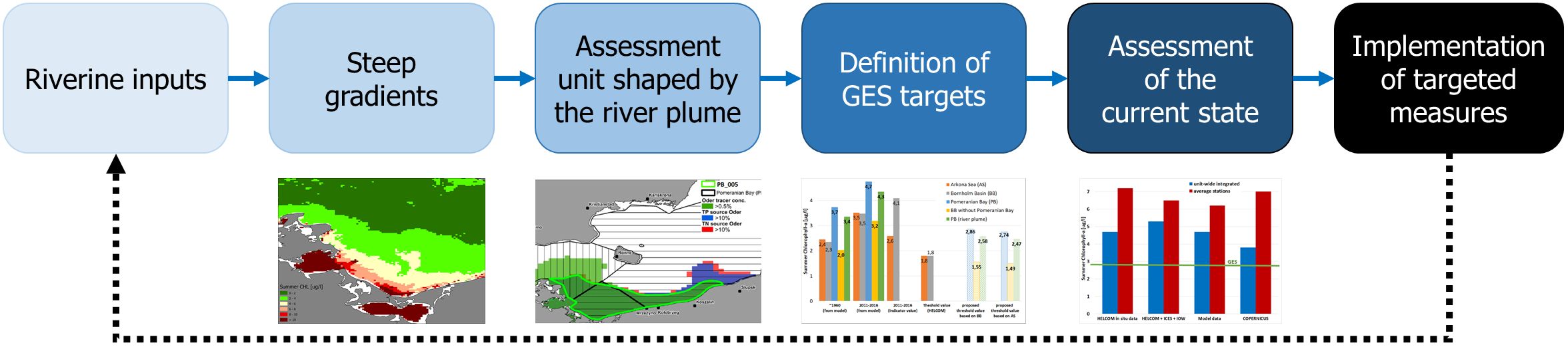
Graphical Abstract.
1 Introduction
Eutrophication is a key anthropogenic pressure on marine ecosystems with severe negative impacts on water quality, biodiversity and the provision of ecosystem services. As a result, it is addressed at multiple governance levels from the global scale (see UN SDG14; Guterres, 2018) and the European perspective via EUs Marine Strategy Framework Directive (MSFD; 2008/56/EC) and EUs Water Framework Directive (WFD; 2000/60/EC). The international regulations are complemented by the work of regional sea conventions, such as HELCOM (the Baltic Marine Environment Protection Commission, also known as the Helsinki Commission) and OSPAR (the successor of the Oslo and Paris Conventions, covering the North-East Atlantic) and national action plans, e.g. in Germany (BLANO, 2014) or Denmark (Maar et al., 2016). Regardless of the spatial scale, achieving a good water quality unaffected by eutrophication is a central social and political global objective.
To achieve a better water quality, an iterative assessment cycle is employed, e.g. within EUs MSFD. The key steps in each cycle (Schernewski et al., 2015) are i) evaluating the current state based on recent monitoring data; ii) comparing this present state to environmental target values that define the Good Environmental (Ecological) State (GES); iii) implementing appropriate measures if the GES targets are not met, to ensure that the targets will get achieved in future. A key component of this process is the development of reliable and broadly accepted water quality targets. They are essential for guiding management actions and determining whether potentially costly measures need to get implemented.
Given the diverse natural hydrodynamic and ecological conditions across European seas, it is not feasible to define universal water quality thresholds that represent the boundary between good and not good for all regions. Instead, the seas are spatially subdivided into assessment units, which should be as homogeneous as possible in order to be represented by an unique GES threshold (Brenner et al., 2006; Borja et al., 2016). Finding a suitable number of assessment units involves a trade-off (Stelzenmüller et al., 2015): fewer units are easier to handle, while a larger number of units more accurately captures natural spatial structures and gradients. This makes the definition of consistent and coherent assessment units (in the sense that they are comprehensible, reflect natural conditions, are internally homogeneous and clearly distinguishable from one another) a central challenge for effective water quality management.
Most regional sea conventions have developed tailored methods to delineate the assessment units, reflecting the unique characteristics of each sea. E.g., the North Sea units have been recently refined within OSPAR (Devlin et al., 2023) replacing the previously used national assessment units by the eco-hydrodynamic regions (van Leeuwen et al., 2015). The semi-enclosed Baltic Sea is naturally divided into several deep basins separated by shallow sills (Mohrholz et al., 2015). These natural boundaries have been used to distinguish the units already in the first environmental assessments of the Baltic Sea (HELCOM, 1980, HELCOM, 1986). The 19 units (Figure 1A) used in the latest holistic assessment (HELCOM, 2023) are still mostly aligned with the original ones, while their sizes differ now by two orders of magnitude, ranging from below 1,000 km2 to above 75,000 km2 (HELCOM, 2022c).
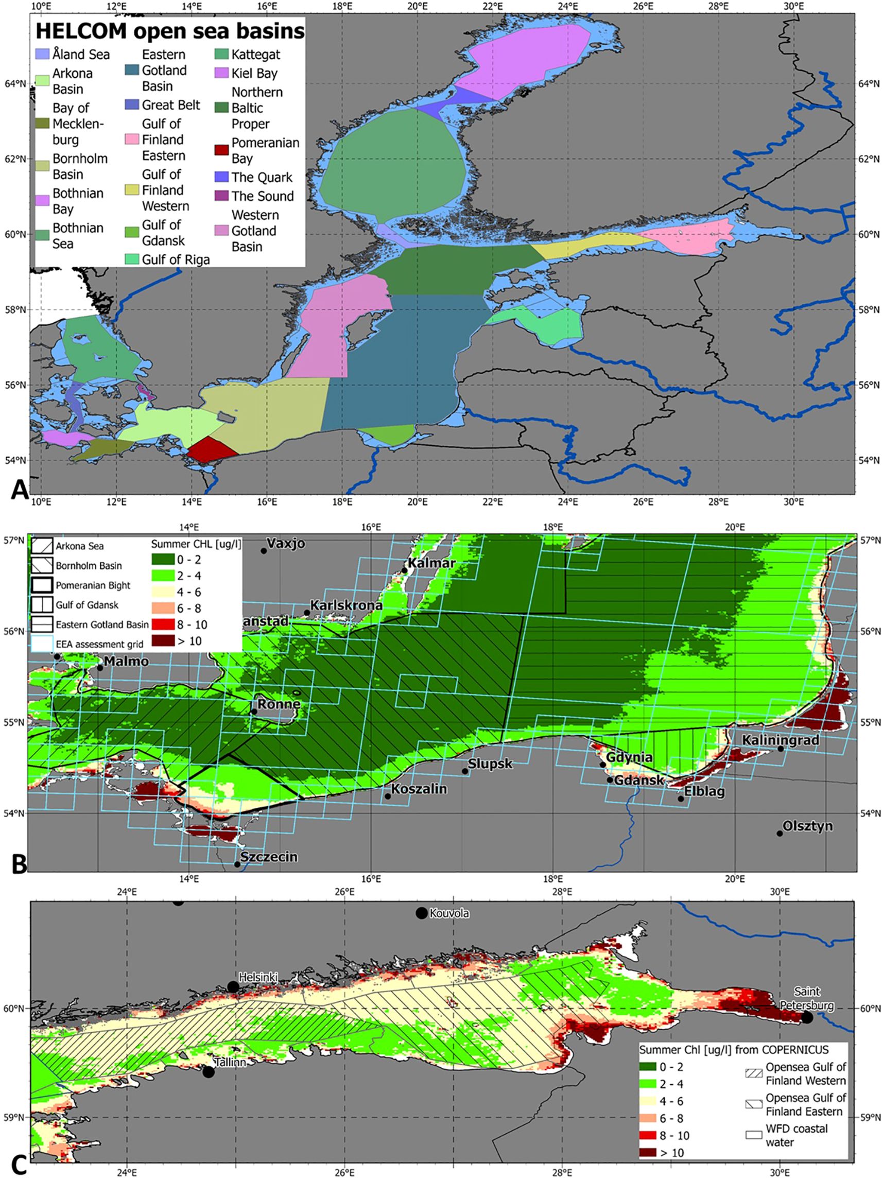
Figure 1. Presently used Baltic Sea assessment units (subfigure (A); open sea parts only) by HELCOM, 2022c; and zoomed into the southern Baltic Sea (subfigure (B); including the assessment boxes of EEA (2019) and into the Gulf of Finland (subfigure (C). The mean Summer chlorophyll-a concentration [ug/l, retrieved from (CMEMS, 2023)] is color-coded.
Despite the refinements, the current HELCOM assessment units do not fully capture the strong gradients observed in all relevant water quality indicators, such as dissolved inorganic nutrients and chlorophyll-a (Figure 1B). This limitation complicates the derivation of representative GES targets and undermines their reliability. Primary driver of these strong gradients and eutrophication itself is the excessive input of nutrients into the seas beyond their natural carrying capacity, mainly due to river inputs (Nixon, 1995; HELCOM, 2022b; Devlin et al., 2023). Areas most affected by riverine inputs exhibit strong spatiotemporal variability, influenced by freshwater runoff, as well as wind- and tide-driven currents (Horner-Devine et al., 2015; Chegini et al., 2020). This dynamic nature makes it difficult to define coherent assessment units for river plume areas. In the North Sea, distinct Regions Of Freshwater Influence have been delineated for major river plumes, such as those of Rhine and Elbe (van Leeuwen et al., 2015). In the Baltic Sea, however, the separation of river plume areas is done only partly. The Gdańsk Basin is separated from the Eastern Gotland Basin (Figure 1B) due to the influence of the Vistula River, one of the largest in the region (HELCOM, 2021a). Similarly, the Gulf of Finland has been split into a western and an eastern section, with the latter more affected by the Neva River plume. However, the line of separation has been chosen quite arbitrary, following the existing WFD coastal assessment units (HELCOM, 2021b) without considering the natural conditions of the open sea water (Figure 1C). Additionally, the HELCOM Bornholm Basin assessment unit has been split into the Pomeranian Bay and the remaining deeper open sea portion, in recognition of the strong natural gradients caused by Oder (Odra) river inputs (HELCOM, 2023). Comparable separations are still lacking for many other Baltic Sea river plume areas, like for the Nemunas, which significantly elevates chlorophyll-a concentrations along the eastern part of the Eastern Gotland Sea assessment unit (Figure 1B).
Once consistent and coherent assessment units and GES targets have been established, the next major challenge in the environmental assessment cycle is to accurately determine the present state of each water quality indicator. This assessment relies on available observations and monitoring data. However, in river plume areas it is often hard to reliably determine the state of the entire assessment unit due to several factors: i) monitoring data points are often highly heterogeneous in time and space; ii) strong gradients caused by the substantial land-based inputs are challenging to capture; and iii) river plumes themselves are not persistent, but highly dynamic and varying over time and space. These challenges can lead to misclassifications and problematic consequences. E.g., if the assessment incorrectly indicates that GES has been reached, necessary management measures will not get implemented. Conversely, a wrong environmental classification results in the implementation of costly but unnecessary measures in the catchment areas, undermining the credibility of the entire assessment cycle. Thus, the combination of heterogeneous monitoring data, deficient GES targets, and inadequately defined spatial units can introduce inconsistencies into the assessment cycle and in the end hinder the progress toward achieving GES.
Effective eutrophication management requires therefore to define coherent assessment units, especially in river plume areas. In addition, it is crucial to establish suitable, consistent, and harmonized GES targets, as well as robust methods to determine the present state of all relevant indicators, despite the challenges posed by data heterogeneity and natural gradients. Using the Oder river plume area in the southern Baltic Sea as a case study, our study aims to: i) present a model-based method to delineate the area most affected by the river plume and its associated nutrient inputs; ii) assess the spatio-temporal variability of the river plume area; iii) propose an assessment unit layout that reflects the influence of the river plume; iv) suggest coherent GES targets for the assessment unit with respect to key water quality indicators; and v) provide a more realistic, integrated estimate of the current state for the entire assessment unit, taking into account the unevenly distributed monitoring stations.
2 Materials and methods
2.1 Model setup
The fully coupled 3D hydrodynamic-biogeochemical model system of the Baltic Sea MOM-ERGOM is utilized to follow the distribution of a passive tracer, which is released with a constant concentration together with the Oder (Odra) freshwater input. The model system covers the whole Baltic Sea (Figure 1) and has a horizontal resolution of three nautical miles and 152 vertical z-layers with thicknesses between 0.5 and 2 m. The physical part of the model is based on the circulation model MOM5.1 (Griffies, 2018; Neumann et al., 2021) and has been adapted to the Baltic Sea with an explicit free surface, an open boundary condition with respect to the North Sea (Neumann, 2021) and freshwater riverine input. Due to the coarse horizontal resolution of the model system (3 nautical miles), the coastal lagoons are included only in a simplified manner. For example, Szczecin Lagoon is only connected the open Baltic Sea via the Swina, while the other outlets are missing. Further, the Swine is too wide in our setup, but the depth is adjusted, so that the mean volume flow out of Szczecin Lagoon into the southern Baltic Sea fits to the observed values (Radziejewska and Schernewski, 2008) or fine-scale model applications (Pein and Staneva, 2024). The passive tracer method is similar to Neumann et al (2017), who implemented a comparable approach to follow the fresh oxygen inputs of a major Baltic inflow. In contrast to Neumann et al (2017), we remove the tracer slowly from the model, using a constant decay rate of 2.7e-3 d-1. This reflects the idea that the impact of the river water and pollutants imported with it becomes weaker over time. The method allows further to compute the age of the river tracer in the marine environment and estimate how long a certain pollutant is already in the system. This makes it possible to identify the area, where the pollutant might still be a hazard before it vanishes or gets inactive. In addition to the passive freshwater tracer, results of Radtke et al (2012) are incorporated. The authors applied a tracing method that allows to follow the nutrient inputs (nitrogen and phosphorus individually) of the Oder (and other sources), e.g., to analyse how they get transported in the Baltic Sea, where they get bound in the lower trophic food web and what their sinks are (Allin et al., 2017).
The model simulation is evaluated for the period 1948–2019 and includes all major water quality indicators, for which GES targets are defined (Schernewski et al., 2015). These are the near-surface concentrations of chlorophyll-a (evaluated only during the growing season May to September, cumulated as Summer chlorophyll-a), Dissolved Inorganic Nitrogen (DIN) and Dissolved Inorganic Phosphorus (DIP, both only evaluated for December to February and cumulated as Winter DIN and Winter DIP), as well as Total Nitrogen (TN) and Total Phosphorus (TP, both annually averaged). The model results have been largely validated with observations previously (e.g. at Eilola et al., 2011; Neumann et al., 2017; Meier et al., 2018; Neumann et al., 2021; Piehl et al., 2022). It also has been shown that the model system is capable to reproduce the long-term developments of the water quality indicators, including the transition of the Baltic Sea open sea waters from oligotrophic or mesotrophic to eutrophic (Neumann and Schernewski, 2008; Voss et al., 2011). Atmospheric forcing of the model is based on a dynamical downscaling provided by the coastDat data set (Weisse et al., 2009; Geyer, 2014). Freshwater inputs and nutrient loads from all 356 reported rivers to the Baltic Sea have been compiled in accordance to recent HELCOM assessments (e.g., HELCOM, 2021a, HELCOM, 2022b) and are based prior to 1995 on the reconstructed riverine loads provided by Gustafsson et al. (2012). Atmospheric nitrogen deposition is prescribed according to EMEP (Gauss et al., 2021) and is based prior to 1995 on the reconstructed deposition from Ruoho-Airola et al. (2012).
2.2 Statistical analysis
To test if the newly introduced assessment unit for the Pomeranian Bay better reflects the spatial variability, we compute the effect size η2 with a one-way ANOVA (Specchiulli et al., 2010; Martínez et al., 2015). To do so, we have interpolated the analysed spatial fields to the assessment unit layouts. This results in an artificial increase in sample size, which not affects the effect sizes (η²), while P-values become unrealistically small (all below 0.001). For the statistical analysis, we use DIN, DIP and chlorophyll-a from three different data sources, which all cover the Southern Baltic Sea completely: Estimates from remote sensing (Brando et al., 2021; CMEMS, 2023; only for the mean chlorophyll-a concentration), the Baltic Sea Biogeochemical Reanalysis (CMEMS, 2024), and our own model results. The parameter η2 describes the fraction of the variance that occurs between the assessment units rather than within them. We calculate this parameter for a two-unit layout (using Arkona Basin and the original unsplitted Bornholm Basin) and a three-unit layout (coastal part of Bornholm Basin referring to Pomeranian Bay, the remaining parts of Bornholm Basin and Arkona Basin after cutting out Pomeranian Bay). For the three-unit layout, we test different separation lines between the coastal and the offshore unit to see which of these gives the highest η2. The aim is to generate assessment units that exhibit as much spatial heterogeneity as possible between them, while ensuring minimal internal variability within each unit. An effect size η2 above 0.14 or 0.06 indicates that splitting the region into three assessment units has a strong or medium effect, respectively (Cohen, 2013).
All maps were created using ArcGIS 10.8.1, all other plots are produced with Matlab, 2021a, using partly the bplot add-on (Lansey, 2023). The spatial interpolation of the monitoring station data is done with the linear 2D-interpolation function interp2 (Matlab interp2, 2025). The interpolation grid covers the Pomeranian Bay and its surroundings and has an evenly spaced grid with a horizontal resolution of 1 km.
2.3 Case study site
To account for a river plume, the new assessment unit Pomeranian Bay has been splitted from the Bornholm Basin assessment unit by HELCOM. The former is supposed to represent the region most affected by the Oder river plume. The Oder river is supplying 60,000 t TN and 3,000 t TP per year to Szczecin Lagoon (Friedland et al., 2019), from where a large part is exported into the southern Baltic Sea (Voss et al., 2010; Friedland et al., 2019). This amplifies the natural gradients between the well-mixed coastal waters and the permanently stratified deep waters even further (Reissmann et al., 2009). The stations with highest concentrations of dissolved inorganic nutrients and chlorophyll-a are located in very shallow waters (Figure 2) without being representative for the entire undivided Bornholm Basin assessment unit. For example, stations 67BC (8.2 m depth), OMOB4 (11.4 m) or 6799 (11.9 m) are substantially below the mean depth of the original assessment unit (46.5 m, standard deviation 23.0 m; Seifert et al. (2001); a detailed bathymetric map of the region is shown by Piehl et al. (2022)). These non-representative stations have seriously affected previous eutrophication assessments, as they are strongly influenced by the Oder river plume. Splitting the assessment unit into two parts have had already an effect for the latest holistic assessment of the Baltic Sea (HELCOM, 2023) where the Bornholm Basin (without Pomeranian Bay) is exceeding the GES target by approximately 53%, while it had shown more than 127% exceedance in the previous assessment for the unsplitted Bornholm Basin (HELCOM, 2018e). The shape of the new assessment unit (Figure 1A) follows the existing boundary to Arkona Basin and the exclusive economic zone boundary of Denmark and is extended eastward to the mouth of river Rega (HELCOM, 2022a). The shape of the new assessment unit considers no further background information, like bathymetry or habitats, and is purely based on a subjective estimate of the area most affected by the Oder.

Figure 2. Key water quality parameters [subfigure (A) Summer chlorophyll-a; subfigure (B) Winter DIN; subfigure (C) Winter DIP] for the monitoring stations in the southern Baltic Sea. Observational data is color-coded for the different assessment units and enhanced by model data (red). The presently valid GES threshold concentrations for the unsplitted Bornholm Basin are highlighted (green).
The present indicator threshold concentrations (serving as GES targets) of the undivided Bornholm Basin assessment unit and the Arkona Basin for Winter DIN, Winter DIP and Summer chlorophyll-a (Supplementary Table ST1 in the Supplementary Material) are following the indicator approach of HELCOM (HELCOM, 2018a, HELCOM, 2018b, HELCOM, 2018c). For the Total Nitrogen (TN) and Total Phosphorus (TP) concentrations (annually averaged) there are no common GES thresholds adopted for the whole south-western Baltic Sea yet. Instead, different thresholds are proposed (Supplementary Table ST2 in Supplementary Material): i) within HELCOM TARGREV (HELCOM, 2013), ii) by Germany (HELCOM, 2016a), and iii) by Poland (HELCOM, 2016b).
Figure 2 shows a comparison between the near-surface dissolved inorganic nutrients and chlorophyll-a concentrations from the regular monitoring stations in the southern Baltic Sea and the model results for the period 2011-2016. Observational data is collected from the ICES database (ICES, 2020), HELCOM Maps and Data service (HELCOM, 2018d) and the database of the Leibniz Institute for Baltic Sea Research Warnemünde (IOW, 2023). chlorophyll-a concentrations from remote sensing have been retrieved from the EU Copernicus service (CMEMS, 2023).
3 Results
3.1 Analysis of the river plume
Using the passive tracer linked to the riverine inputs of the Oder (Odra) allows to identify the average spatial extent of the river plume area, but also how far it spreads into the open Baltic Sea during certain events (Figure 3). The river tracer concentration is highest in Szczecin Lagoon, but it reaches high mean values in the Arkona Basin and along the Polish coast far beyond the new HELCOM Pomeranian Bay assessment unit. The maximal extent of the river plume (using as threshold of 1% compared to the concentration at the river mouth) is reaching up to the coasts of Denmark and Sweden, as well as into Gdańsk Basin (Figure 3). The tracer shows a strong spatial variability, e.g. the plume is pushed towards the southern shore in September 2006, when first northerly winds and afterwards easterly winds dominate (Supplementary Figure S1 in the Supplementary Material). This period is characterized by unusually high chlorophyll-a concentrations in the southern part of Pomeranian Bay, while the offshore concentrations are below the September mean value (Supplementary Figure S2 at Supplementary Material). The tracer distribution shows a completely different pattern in August 1980, when the river plume is transported far east, resulting in much higher concentrations due to a long-lasting period with prevailing westerly winds (Supplementary Figure S1 at Supplementary Material). Overall, the river tracer concentrations show a wide range of values for the monitoring stations in the southern Baltic Sea. The stations with the highest mean (and median) concentrations are all located in the new HELCOM assessment unit Pomeranian Bay, indicating the permanent influence of the river plume at the stations closest to the river mouth. Nevertheless, stations which are in the remaining part of the Bornholm Basin or the Arkona Basin (like ST6799, OMO11 or TF152), also show high concentrations of the river tracer. With decreasing concentrations of the river tracer the spread between the mean and the median values mostly increases.
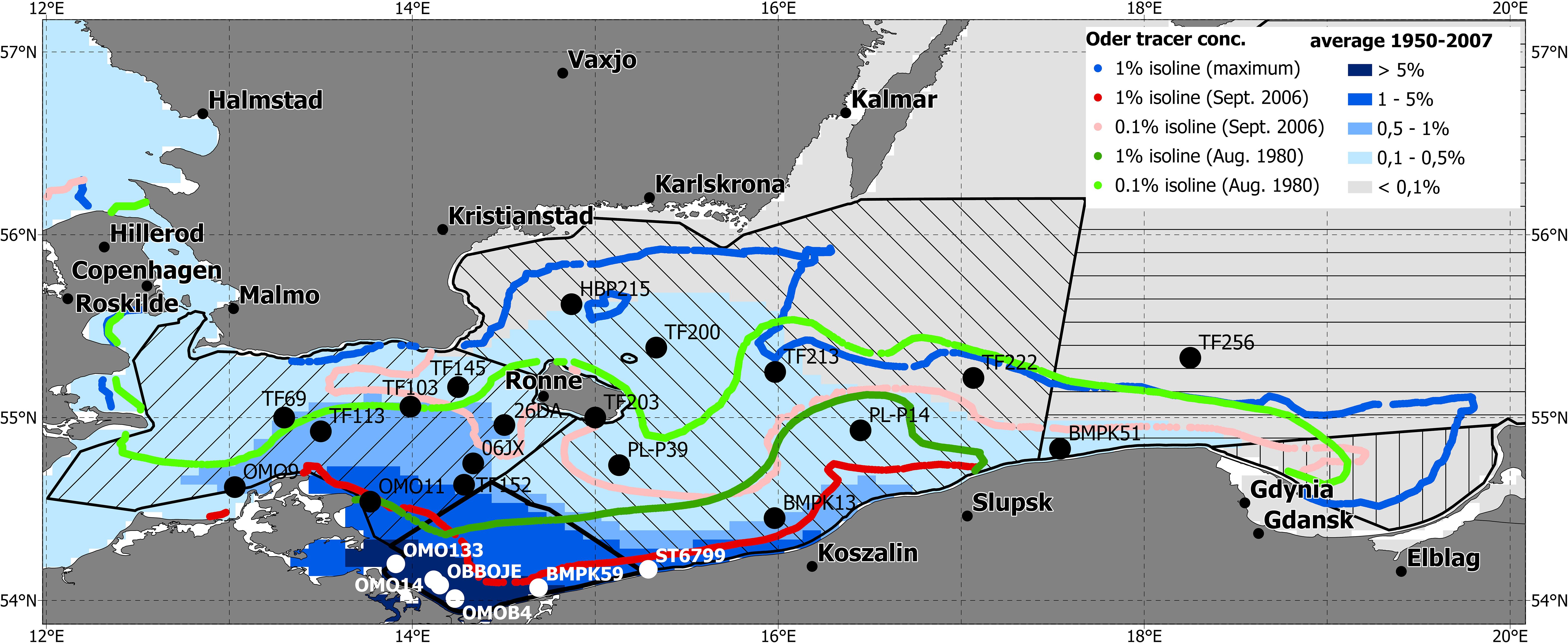
Figure 3. Distribution of the Oder river tracer (scaled to 100% at the river mouth) and the monitoring stations (white and black dots). The colour scale represents average values over the simulation period. The blue contour line indicates the maximal distribution, where still 1% of the tracer occurred. The red and green isolines reflect single events from August 1980 (green) and September 2006 (red) at different intensities (light and dark contours are 0.1% and 1% isolines, respectively). Hatched are the currently used HELCOM assessment units in the Southern Baltic Sea (see (Figure 1A).
The annual mean extent of the region most affected by the river Oder plume (defined by tracer concentrations of at least 1%) is varying between approx. 5,000 and 11,000 km2 (Supplementary Figure S3 at Supplementary Material). There is a strong inter-annual variability of this area, which is closely related to the freshwater runoff of the Oder with a phase shift of approx. five months (Supplementary Figure S4 at Supplementary Material). Despite the impact of the prevailing winds on the shape of the river plume during certain events (Figure 3), there is only a weak correlation between the extent of the area with a river tracer concentration above 1% and the wind components (Supplementary Figure S5 at Supplementary Material). There is a negative correlation with northerly winds, which is highest at a phase shift of 78 days, indicating that northerly winds diminish the river plume area. The correlation of the area to westerly winds is even weaker and the time lag was below 10 days (Supplementary Figure S5 at Supplementary Material). The mean age of the river tracer (Supplementary Figure S6 at Supplementary Material) is mostly below two years in the south-western part of Bornholm Basin, while it reaches up to four years in Arkona Basin and along the Polish coast. There is a high correlation between the river tracer concentration and its age (R=-0.95), due to the supply of new river tracers with age 0. Although the region with the average age below two years is mainly bound to Pomeranian Bay, it can stretch up to the coasts of Denmark and Sweden, as well as into Gdańsk Basin (Supplementary Figure S6 at Supplementary Material).
The river Oder is the major source of nutrients in the southern Baltic Sea. For most of the area and monitoring stations, the Oder is the source of up to 50% of the nutrients found in the water column (Figures 4, 5). The region with the highest impact of the Oder inputs is stretching up to Rügen Island and along the Polish coast. For the later area the nutrient source allocation values are above the pure river tracer concentrations (e.g. visible at stations BMPK13 or PL-P14), indicating that the nutrients are transported further after getting incorporated into the food web. The spatial gradients of the source appointment differ only minor between nitrogen and phosphorous, as long as values are high (above 10%). On the other hand, the area, where the Oder is the source for at least 5% of the TP, extends significantly more into the open Baltic Sea (Figure 4) than the corresponding region for TN, which is mostly bound to the near-coastal areas.
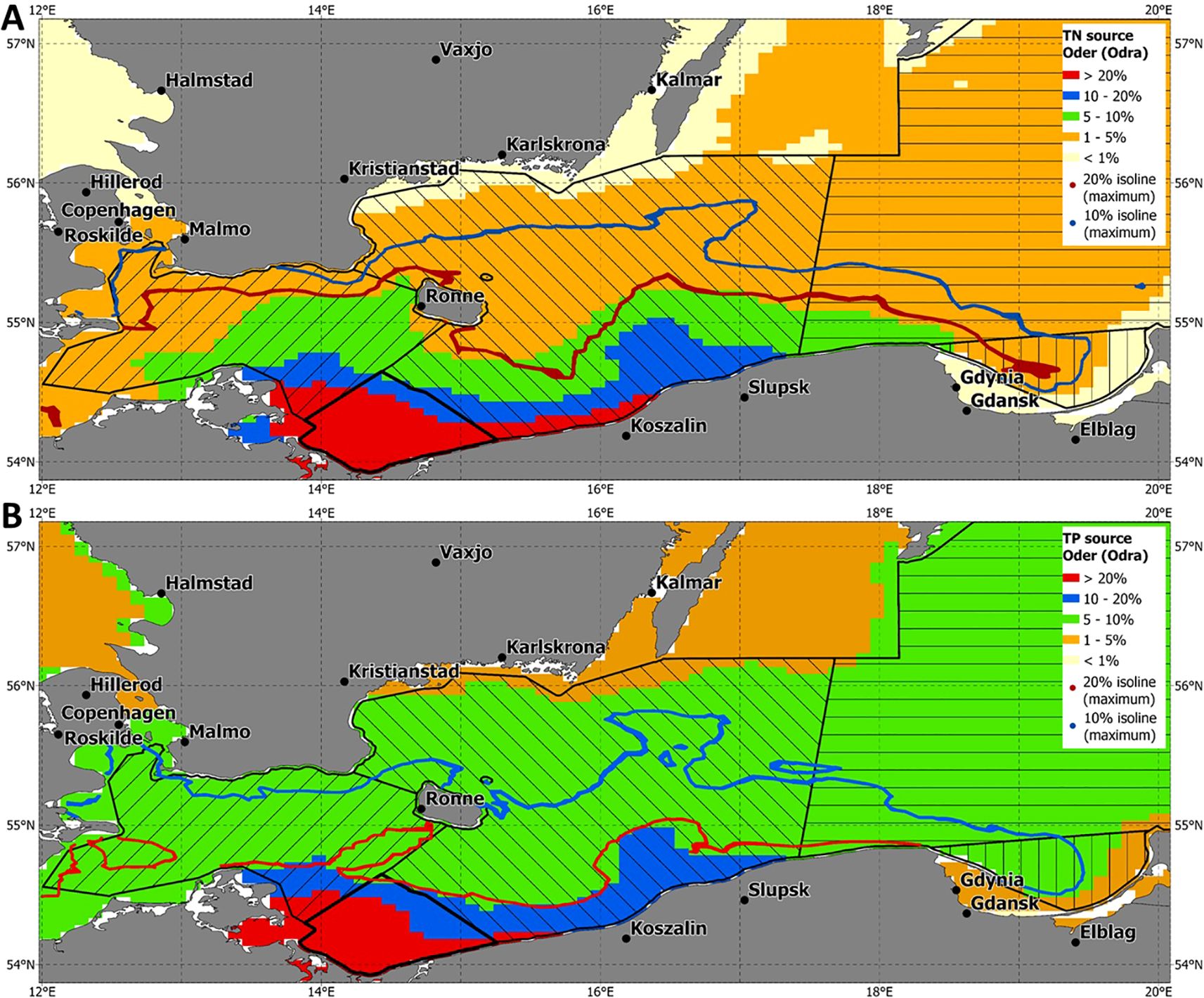
Figure 4. Source attribution of Total Nitrogen (subfigure A) and Total Phosphorus (subfigure B) with respect to inputs from Oder river, illustrating that it is the dominant nutrient source in the southern Baltic Sea. The colour scale represents mean values, while red and blue isolines indicate the maximal spatial extent where the Oder contributes at least 20% and 10% of the nutrient load, respectively. Hatched are the currently used HELCOM assessment units in the Southern Baltic Sea (see Figure 1A).
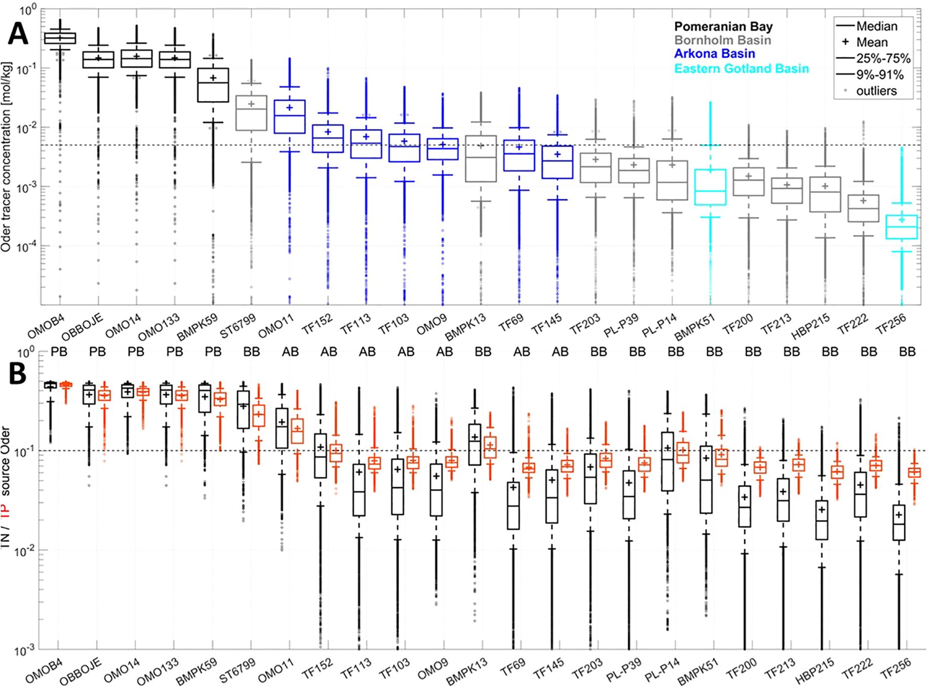
Figure 5. River tracer concentration (subfigure A) and source attribution (subfigure B) black: Total Nitrogen inputs; red: Total Phosphorous inputs) with respect to inputs of Oder river for selected monitoring stations. The dotted lines mark 0.5% (subfigure A) and 10% (subfigure B), respectively. Abbreviations indicate the HELCOM assessment unit, in which each station is located (PB, Pomeranian Bay; BB, Bornholm Basin; AB, Arkona Basin).
3.2 Shaping the assessment unit on the basis of the Oder river plume
Combining the Oder (Odra) river tracer (Figure 3) with the region, where the Oder is the most important nutrient source (Figure 4), allows to transfer the river plume into a designated assessment unit purely shaped by the river plume. Using both components is beneficial as for some monitoring stations (like BMPK13 or PL-P14) the Oder nutrient impact is more pronounced compared to the pure plume tracer (Figure 5). In Figure 6 different layouts of possible Pomeranian Bay assessment units shaped by the river plume are shown using various thresholds of both components. River tracer concentration thresholds vary between 0.2% and 5% and the nutrient source allocation thresholds between 5% and 20% (Table 1; Figure 6B). The potential layouts extend between 1,300 km2 (PB_05) and 18,200 km2 (PB_002; the HELCOM assessment unit has approx. 4,000 km2; Table 1) and differ substantially with respect to the amount of the stored Oder river tracer (Figure 6C). The mean values rise from approx. 40% to 45% (PB_01) and even up to 60% (PB_002). Only in the layout with the highest threshold values (PB_05) the amount of Oder river tracer stored in this area decreases to approx. 30%, being even lower than for the HELCOM assessment unit. Figure 6A shows in detail how the PB_005 layout is shaped, if the river tracer concentration exceeds 0.5% (green area) and the Oder is the source for at least 10% of the nutrients (red and blue areas). The PB_005 layout incorporates the new HELCOM assessment unit, but it includes also the south-eastern part of Arkona Basin and stretches along the Polish coast up to 16.7°E. The PB_005 layout is not including some parts of Arkona Basin, although the river tracer concentration is still quite high there. Here, the Oder river becomes a too small nutrient source (light green in Figure 6A). Vice versa, the area along the Polish coastline north-west of Słupsk is not included, although the Oder is still the major nutrient source (blue and red in Figure 6A), while the river tracer concentration is already quite low and only exceeding the threshold if certain weather conditions occur (see Figure 3).

Figure 6. Definition of layout PB_005 (green contour line; subfigure A) based on the modelled distribution of the Oder tracer of at least 0.5% (green area) and the nutrient source appointment of at least 10% (red and blue areas). Hatched are the Pomeranian Bay, Arkona Sea and Bornholm Basin assessment units of HELCOM. The different layouts of the river plume area tested with the ANOVA depending on the chosen thresholds for the river tracer as well as the river nutrient source allocation (subfigure B) thresholds are in Table 1) the ratio of the amount of the river tracer found in the Pomeranian Bay assessment unit from HELCOM (black) in comparison to our layouts with the tracer found in the entire Baltic Sea (subfigure (C).
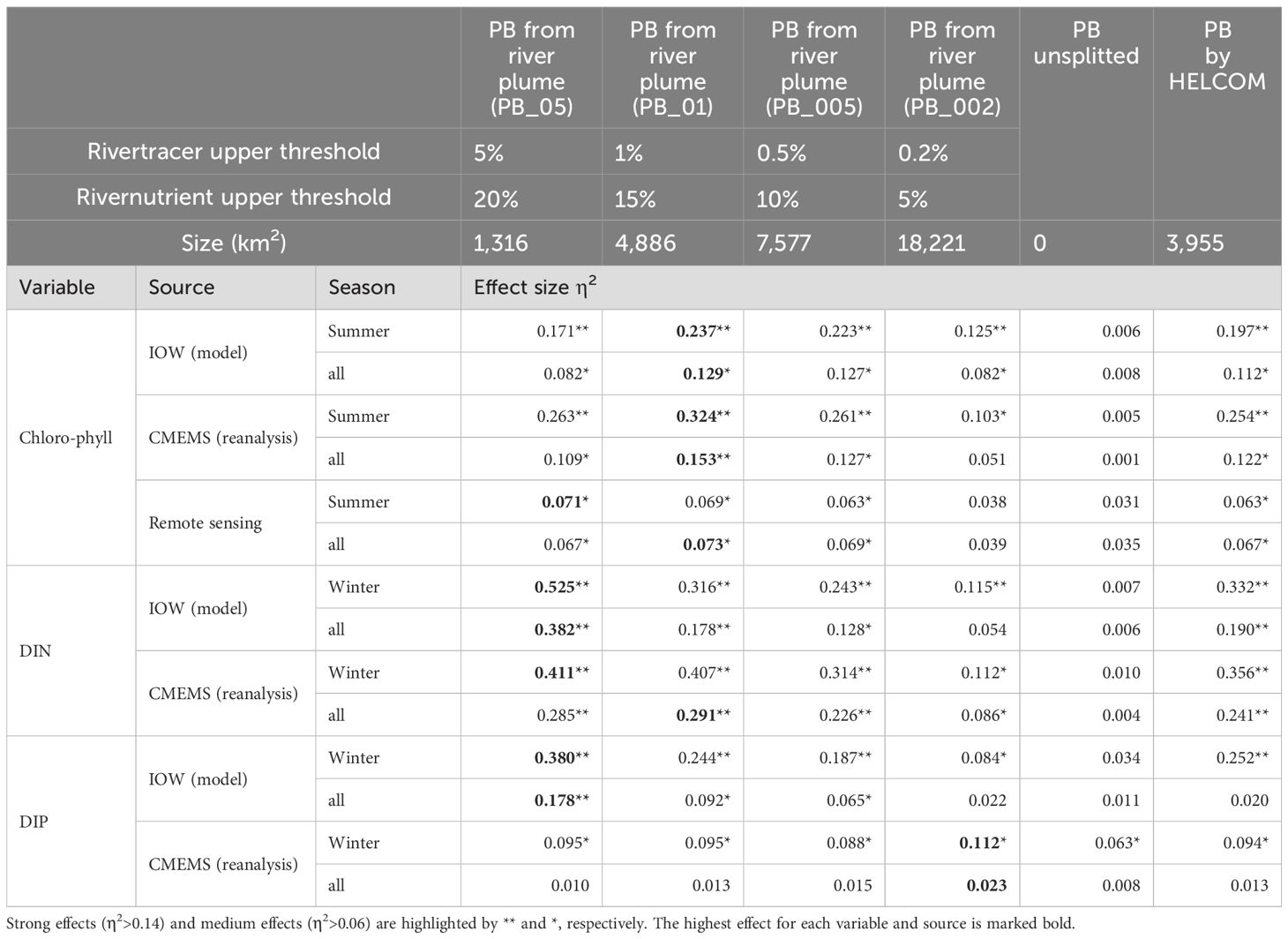
Table 1. Effect sizes (η2) for different layouts of the Pomeranian Bay (PB) assessment unit computed for chlorophyll-a, dissolved inorganic nitrogen (DIN) and dissolved inorganic phosphorus (DIP) taken from the ERGOM-MOM simulation (IOW model), the CMEMS reanalysis (CMEMS, 2024) and remote sensing (CMEMS, 2023).
To estimate how the different layouts of the assessment units change the spatial heterogeneity, a one-way ANOVA is conducted for three water quality indicators, using the dissolved nutrients and chlorophyll-a from our own model, a reanalysis product and for chlorophyll-a also from remote sensing (results are shown in Table 1). For all variables the effect sizes η2 are lowest when no Pomeranian Bay unit is introduced and increase if the additional assessment unit is included. Generally, the effect sizes for the remote sensing product are substantially lower than for the model and reanalysis results. For all three variables the effect size for at least one of our layouts is higher than for the HELCOM assessment unit, indicating that the HELCOM approach to delimit the region is not optimal. The results differ substantially between the different variables, but also between the periods during which these variables are evaluated. During the seasons that are presently used for the water quality assessments, the values of η2 are nearly always larger than for the whole-year period, indicating that the spatial pattern is more pronounced in the assessment periods (Table 1). The effect sizes are overall highest for DIN, which shows the strongest spatial gradient. For DIN the maximum effect size is gained by the PB_05 layout, which is the unit restricted most to the river mouth (Figure 6B). For DIP this holds also for the IOW model results, while it is reversed for the CMEMS reanalysis, where the PB_002 layout gains the highest effect size. Overall, the differences between the layouts are less strong for DIP than for DIN. Besides, the effect size is only classified as medium and not as strong for most of the other variables. For chlorophyll-a, the intermediate layout PB_01 (but also PB_005) gains the highest effect sizes, indicating that including more of the offshore waters enhances the spatially homogeneity.
Combining the results for the different tested layouts and water quality indicators, PB_01 seems overall well suitable as Pomeranian Bay assessment unit. It has higher effect sizes than the layouts with lower thresholds (PB_005 and PB_002; except for DIP from the CMEMS reanalysis). With respect to chlorophyll-a it is also better than PB_05, although this layout gains higher effect sizes for Winter DIN and Winter DIP. Nevertheless, PB_05 is by far the smallest assessment unit, containing only a comparably low fraction of the river tracer (Figure 6C), thus the risk stays high that the remaining part of Bornholm Basin gets again falsified water quality assessment results. Therefore, the intermediate layout PB_01 seems best to shape the assessment unit following the river plume.
3.3 Provision of GES targets for the new assessment unit
Using a long-term simulation of the IOW model ERGOM-MOM (Figure 2), allows to compute the assessment unit wide spatial means for Summer chlorophyll-a, Winter DIN and Winter DIP, and how these key water quality parameters have developed since the pre-eutrophic period around 1950. The spatial averages of key water quality parameters are calculated from the IOW model results for the Arkona Basin and the unsplitted Bornholm Basin, for the new Pomeranian Bay assessment unit implemented by HELCOM and for the remaining part of Bornholm Basin after cutting out the Pomeranian Bay, as well as for PB_01 layout shaped by the river plume (Figures 7–9). Following the natural gradients, all water quality indicators are substantially higher in both Pomeranian Bay units than in the other assessment units and become remarkably lower for the Bornholm Basin after cutting out the Pomeranian Bay assessment unit.

Figure 7. Long-term development of Summer chlorophyll-a computed with ERGOM-MOM for the different assessment units (subfigure A) and mean Summer chlorophyll-a concentrations computed for the different assessment units and assessment periods based on model results from ERGOM-MOM (subfigure B). HELCOM indicator data (HELCOM, 2018a) and proposed thresholds for the new assessment units are based on the existing GES targets for Bornholm Basin and Arkona Basin.
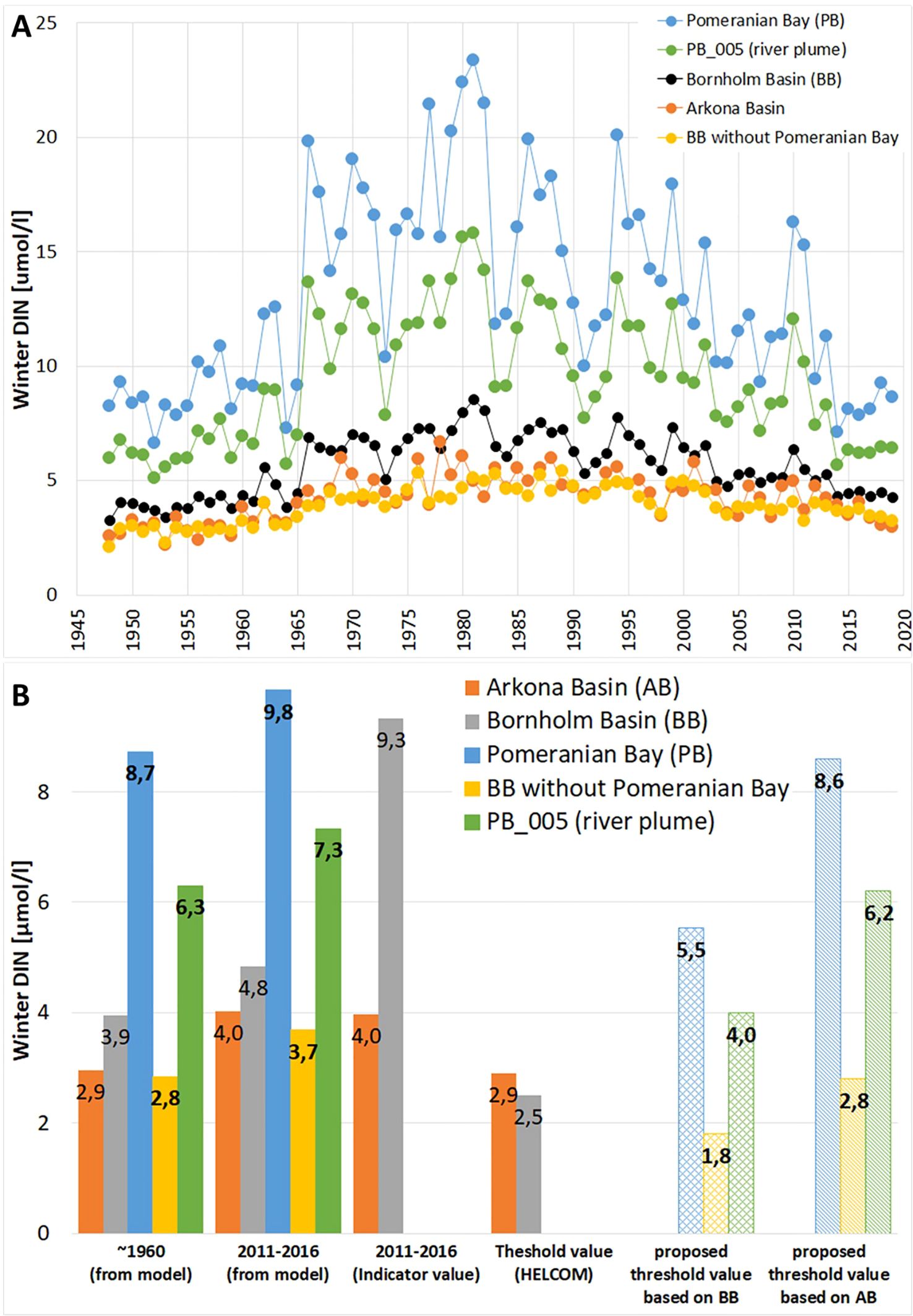
Figure 8. Long-term development of Winter DIN [umol/l] computed with ERGOM-MOM for the different assessment units (subfigure A) and mean Winter DIN concentrations computed for the different assessment units and assessment periods based on model results from ERGOM-MOM (subfigure B), HELCOM indicator data (HELCOM, 2018b) and proposed thresholds for the new assessment units are based on the existing GES targets for Bornholm Basin and Arkona Basin.
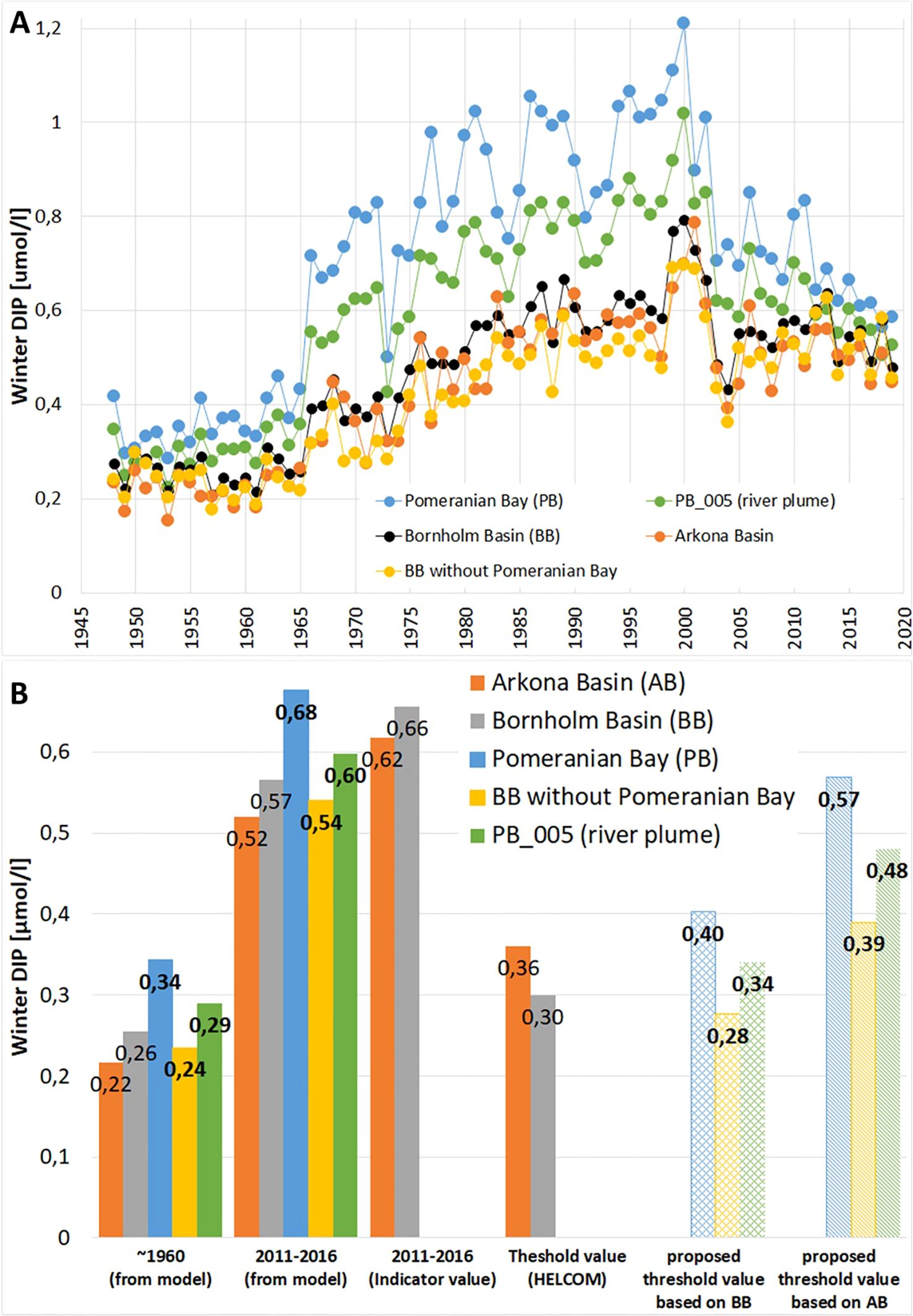
Figure 9. Long-term development of Winter DIP [umol/l] computed with ERGOM-MOM for the different assessment units (subfigure A) and mean Winter DIP concentrations computed for the different assessment units and assessment periods based on model results from ERGOM-MOM (subfigure B). HELCOM indicator data (HELCOM, 2018c) and proposed thresholds for the new assessment units are based on the existing GES targets for Bornholm Basin and Arkona Basin.
Using the long-term time series of the different spatial means of the Pomeranian Bay unit (PB) and the unsplitted Bornholm Basin (BB), the ratios between the water quality parameters of both can be computed as c_PB/c_BB with c being the mean concentration of Winter DIN, Winter DIP or Summer chlorophyll-a. The ratios decrease noticeable from pre-eutrophied state (1950s and 1960s) until today (e.g. from 1.53 to 1.36 for Summer chlorophyll-a; Table 2). This indicates that the eutrophication pressure is pushed from the near-shore area towards the open sea basin during (but also after) the period with the highest riverine nutrient inputs.

Table 2. Ratios of the spatial averages of summer chlorophyll-a, winter dissolved inorganic nitrogen (Winter DIN) and winter dissolved inorganic phosphorus (Winter DIP), as well as total nitrogen (TN) and total phosphorus (TP; both annually averaged) computed from the ERGOM-MOM simulation evaluated for the assessment unit for the Pomeranian Bay (PB, as suggested by HELCOM) compared to the original Bornholm Basin (BB) as well as for the river plume shaped Pomeranian Bay unit (using PB_005 layout) also compared to the original (undivided) Bornholm Basin (BB).
Using the ratios of the spatial means from the time-period still unaffected by eutrophication around 1960 as scaling factors (Table 2) allows to transmit the already harmonized and coordinated GES threshold values for Summer chlorophyll-a, Winter DIN and Winter DIP of the original Bornholm Basin to the new Pomeranian Bay assessment unit. The same procedure is applied to the remaining part of Bornholm Basin after cutting out the HELCOM Pomeranian Bay unit, as the residual open sea part has remarkably lower concentrations of all key water quality indicators. The transfer factor from the unsplitted Bornholm Basin to the new assessment units varies strongly between the water quality indicators (Table 2). For Winter DIN the transfer factor is especially high, reflecting the strong natural gradients between the river plume area and the open sea waters.
Applying the described procedure results in a GES threshold for Summer chlorophyll-a of 2.86 ug/l for the HELCOM Pomeranian Bay and 1.55 ug/l for the residual Bornholm Basin, which previously had 1.8 ug/l as GES threshold (Figure 7B). For Winter DIN (Figure 8B) and Winter DIP (Figure 9B), the suggested GES thresholds for the Pomeranian Bay units are significantly higher than for Bornholm Basin or Arkona Basin. Using the existing GES threshold value of Bornholm Basin as basis for the new assessment units results in quite low threshold concentrations for Winter DIN (Figure 8B). These are substantially below the model-based spatial means, even of the pre-eutrophic period, in the Pomeranian Bay as well as in the residual part of Bornholm Basin. Using instead the GES thresholds of Arkona Basin, which are substantially higher than for the unsplitted Bornholm Basin, as basis for the transmitting procedure, results in GES threshold suggestions for Winter DIN (8.6 umol/l for PB and 2.8 umol/l for the remaining part of BB) that are quite close to the modelled spatial means around 1960 (Figure 8B). For Winter DIP (Figure 9) the original procedure to base the new GES thresholds on the one for the unsplitted Bornholm Basin, resulted in GES values quite comparable to model-based spatial means of the state around 1960 (0.4 umol/l for Pomeranian Bay and 0.28 umol/l for the remaining part of Bornholm Basin). Currently, there are no GES thresholds defined for TN and TP concentrations of the unsplitted Bornholm Basin. Instead, different GES targets are proposed (Supplementary Table ST2 in Supplementary Material). Using each of them results in a different GES threshold for the new Pomeranian Bay assessment unit with GES thresholds between 19.1 and 23.8 umol/l TN as well as 0.68 and 0.77 umol/l TP.
3.4 Indicator status assessment of the new assessment unit
Using purely the observations from the available stations (from HELCOM, ICES and IOW´s database; Figure 10) to estimate the spatial mean of the Pomeranian Bay assessment unit results in a present state that is not considering the natural gradients, as the monitoring stations are only located along the shoreline. It is instead only reflecting the high, near-shore concentrations (Figure 3).
To overcome this problem aiming to gain a more realistic present state which includes also the unmonitored open sea part of the assessment unit, we interpolate the station data spatially including also observations from the surrounding assessment units. The results are shown in Table 3. Computing the regional average out of the spatially interpolated fields results in much lower values for all water quality indicators independent if in situ data, model results or remote sensing product are used. Only for Winter DIP, the differences are quite marginal, as concentrations show only a weak gradient (Figure 2). Independent from the assessment method and the data source, all current state values are strongly above the proposed GES thresholds for the whole Pomeranian Bay assessment unit.

Table 3. Assessment of the mean state (2011-2016) for the assessment unit, comparing averages based on spatial interpolation of station data with those calculated only by averaging the station data within each assessment unit.
4 Discussion
4.1 Delineate assessment units shaped by river plumes
Defining spatial management units in marine waters is highly challenging (Melaku Canu et al., 2024). While we utilize a model-based approach to find the best layout of an assessment unit following a river plume, other approaches are common. For example, the European Environmental Agency applies a standardized approach for all European seas (EEA, 2019) by dividing each sea into equally sized horizontal boxes (Figure 1B; EEA, 2018). While this method is easy to implement, it does not account for spatial gradients or natural structures. In addition, the regular monitoring does not always match the EEA grid, leaving many grid cells with insufficient observations. This approach creates a large number of assessment units, making it hardly possible for managers to track the results for all units. Regional approaches, such as those used by OSPAR or HELCOM, seem more convenient, because their assessment units base mostly on scientific principles. However, also other factors, like historical aspects, data availability, political interests, and demarcations, influence how the units are defined.
Despite being largely impacted by riverine freshwater and nutrient inputs, river plume areas are often merged with offshore marine waters in the assessments. Using the Pomeranian Bay and the Oder (Odra) river plume as case study, we show by utilizing both, a freshwater tracer and a nutrient source allocation, where the river-borne nutrients and pollutants affect marine water quality most. Since these two components influence water quality on different temporal and spatial scales, both should be considered when delineating assessment units related to river plumes. By adding a passive tracer to the Oder freshwater inputs, we follow the extent of the river plume as well as its movement over space and time (Figure 3). Although the assumed constant tracer decay rate has only a minor effect on the spatial gradients from the river mouth to the open sea, it may need to be adjusted if the tracer is intended to mimic also the gradual breakdown in the marine environment of a specific pollutant. The size and shape of the river plume depends on both wind conditions and freshwater inflow. The wind affects the plume over short timescales (estimated lag times are ten days for westerly winds and 78 days for northerly winds). In contract, changes in freshwater runoff influence the plume over longer periods with a lag time of around five months. As the concentrations of the river tracer decreases, the spread between mean and median values widens (Figure 5) showing the significant role of individual events in shaping the distribution of plume waters.
A wide variety of possible assessment unit layouts can be derived by applying different threshold concentrations for the passive freshwater tracer and nutrient source allocation (Figure 6B). To decide which layout is optimal, we apply several one-way ANOVAs (using different spatially high resolved water quality indicators as input). Unfortunately, in our case study results differ between the tested input variables. Either a small area limited to the shore is best (when dissolved nutrients are considered), or it extends further offshore, when using chlorophyll-a as indicator. This matches the natural gradients, which are steeper for DIN than for chlorophyll-a (Figure 2), due to the significant impact of Oder nitrogen inputs as well as the high turnover and burial rates of nitrogen in the coastal zone (Allin et al., 2017; Asmala et al., 2017). Nevertheless, implementing one of our proposed layouts (Figure 6B) instead of the HELCOM assessment unit for Pomeranian Bay would allow to delineate management units with greater internal homogeneity and heterogeneity between them. Using a MANOVA (Multivariate analysis of variance; St and Wold, 1990) instead of separate one-way ANOVAs could help managers to identify the best assessment unit layout for all indicators simultaneously, if an unique results is preferred instead of the mixed outcome from the single indicators.
An alternative way to define assessment units shaped by river plumes or other ecological drivers is to consider biotopes (Schiele et al., 2015) or ecoregions (Schaub et al., 2024). In our case study area, this is possible because these natural divisions are well known and allow for clear separation. However, comparable information is often lacking, making it nearly impossible to generalize this approach. Additionally, biotopes and habitats mainly reflect near-bottom ecosystems and do not capture near-surface gradients in key water quality indicators such as dissolved nutrient concentrations. Another possibility is to follow van Leeuwen et al. (2015), who used salinity and stratification intensity to delineate regions of freshwater influence in the North Sea. However, this approach is not appropriate for the Baltic Sea, where salinity naturally decreases (Kniebusch et al., 2019; Lehmann et al., 2022), masking the spatial influence of river plumes on salinity and stratification. Stable isotopes can also trace riverine inputs (Voss et al., 2005), but their analysis is bound to the sea floor and only available for a small number of coastal waters and analysed stations. Remote sensing techniques can be used also to monitor river plumes and their impact on water quality (Devlin et al., 2015) by delineating areas most affected by terrestrial inputs (Haji Gholizadeh et al., 2016). Satellite-derived chlorophyll-a concentrations can be used, but as shown in Table 1, assessment units that are homogeneous for chlorophyll-a are possibly not well suited for other water quality parameters. In future, AI may help to define suitable assessment units by processing complex datasets to identify key spatial patterns (Gambín et al., 2021; Ditria et al., 2022; Uddin et al., 2023). AI can also track changes in environmental conditions over time, capturing spatial and temporal dynamics (Di Ciaccio, 2024). Explainable AI methods may allow to identify river plumes as significant drivers of marine water quality (Nallakaruppan et al., 2024), detect unusual patterns or outliers (Ning et al., 2024), and suggest adjustments to assessment units. Furthermore, AI methods may help to fill gaps in space and time from the regular monitoring (Friedland et al., 2023), leading to more accurate and targeted water quality assessments.
Although our methodology relies on a computationally intensive coupled 3D-model, it can be applied with little effort to other areas. Being strongly affect by rivers (HELCOM, 2021a), the Baltic Sea is well suited as test case, as the river shaped units are defined either arbitrarily (for Vistula and Neva), or are missing (e.g., for Nemunas or Narva). Applying our proposed method would allow for a systematic adjustment of the HELCOM assessment units: first, by separating the specific river plume units, and then by reshaping the remaining open sea basins according to their natural conditions and basin characteristics.
4.2 Derivation of suitable GES thresholds and assessment of the current state
The GES threshold-setting approach presented here is pragmatic and has already got implemented in the recent holistic assessments of the Baltic Sea’s environmental status (HELCOM, 2023). The derived GES threshold concentrations are based on existing values for the old (unsplitted) Bornholm Basin assessment units. These thresholds are transferred to the Pomeranian Bay unit using factors calculated from a long-term model simulation considering the natural gradients (Figures 7–9). The new GES values are substantially higher in the river plume area, while for the remaining offshore part of Bornholm Basin lower (and therefore stricter) ones are proposed, as the most eutrophied part of it is cut out. The simulation shows thereby how the eutrophication pressure is pushed from the near-shore river plume towards the open sea basin during and after the period with the highest riverine nutrient inputs (Table 2). Using spatial ratios from around 1960 as transfer factors is appropriate, as they better represent the GES than those based on the current, highly eutrophied state. Since the transfer factors from the unsplitted Bornholm Basin to the new Pomeranian Bay assessment unit vary significantly, they are determined individually for each water quality indicators. This is necessary, because the transfer factors reflect not only spatial gradients but also the sensitivity of each indicator to changes in nutrient inputs. Dummy
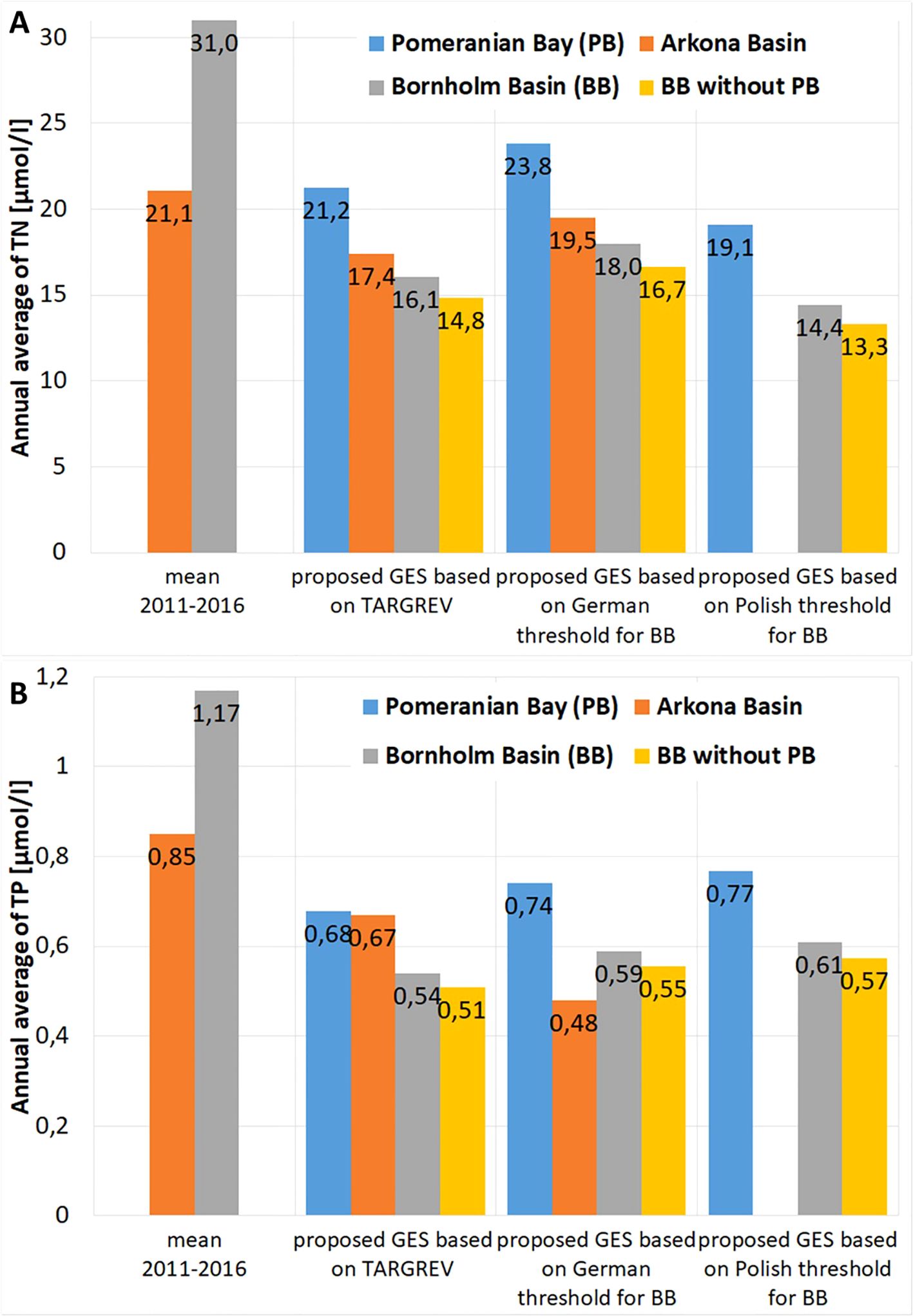
Figure 10. Present state and proposed GES thresholds of the TN (subfigure A) and TP (subfigure B) concentrations (annually averaged) for the existing and the new assessment units based on the TARGREV proposal (HELCOM, 2013) and the German and Polish threshold proposals for the Bornholm Basin (HELCOM, 2016a, HELCOM 2016b) .
Although the proposed target-setting approach is not perfect (for example, it results in an unrealistically low GES target for Winter DIN based on the original Bornholm Basin value; Figure 8B), it is pragmatic, efficient and enables to derive consistent and harmonized GES targets. The new GES thresholds align with natural gradients and are consistent with the existing targets that have been accepted and adopted by all HELCOM member states. However, the method has its limitations. For instance, different GES thresholds for TN and TP are suggested (Supplementary Table ST2 at Supplementary Material), but none has yet been fully implemented by HELCOM for Arkona Basin nor Bornholm Basin. Despite the challenges, the approach seems suitable, as the derived GES thresholds are consistent with those for surrounding open sea units and take into account the natural gradients from river mouths to offshore waters.
For Pomeranian Bay assessment unit, there are alternative ways to derive the GES targets, each with its own strengths and shortcomings. Due to the lack of observations from the pre-eutrophic period, it is not possible to establish the reference state solely on historical data. Using the target-setting approach of Schernewski et al. (2015) would lead to GES thresholds that are harmonized and consistent with those for German Baltic Sea waters, but not with the neighbouring Polish, Danish, and Swedish waters. More sophisticated methods, such as running a large model ensembles to estimate the pre-eutrophic state, like van Leeuwen et al. (2023), are currently not feasible, but will be necessary in the future to overcome the inconsistencies in existing GES targets. Adopting a full ensemble modelling approach, as done in the HELCOM-TARGREV project (HELCOM, 2013), offers the advantage of estimating the pre-eutrophic state with lower uncertainty than any single model. Ensembles further provide more robust results by identifying coherent and consistent patterns across the models (Friedland et al., 2021). However, combining several model systems into an ensemble is highly challenging and requires careful attention to ensure comparability and consistency of the results.
Most long-term monitoring stations in the southern Baltic Sea are located in near-shore shallow waters (Figure 3). Relying solely on observations from these stations to assess the current state of the Pomeranian Bay assessment unit results in an overrepresentation of high near-shore concentrations (Table 3, Figure 10). This leads to unrealistically high values for the entire unit, which are up to 50% higher than, if offshore areas are considered. To fill the temporal and spatial gaps, geostatistical methods or biogeochemical reanalysis products (like CMEMS, 2024) can be used. However, all these approaches are limited by the lack of offshore monitoring data. This gap can only be closed by establishing new monitoring stations in the offshore part of Pomeranian Bay. Model-based techniques can help to identify optimal locations for these new monitoring stations (Ferrarin et al., 2021). Introducing additional offshore monitoring stations will enable more accurate and realistic environmental assessments in the future. However, to understand long-term developments suitable modelling approaches remain essential (Voss et al., 2011).
5 Summary & conclusions
Introducing a river tracer together with the Oder (Odra) river inputs allows us to follow the river plume in the south-western Baltic Sea. Combining the river tracer with the nutrient source allocation of Radtke et al. (2012) and using a one-way ANOVA and the effect size as optimizing criteria, allows us to identify the best assessment unit shape. Although the effect sizes differ between the water quality indicators, we suggest an alternative delineation of the Pomeranian Bay assessment unit compared to the one implemented by HELCOM. Having higher effect sizes, our proposed assessment unit has a higher internal homogeneity and a stronger heterogeneity to the other units. Further, GES thresholds are suggested for Pomeranian Bay and the remaining part of the original Bornholm Basin assessment unit. These GES values take into account the natural gradients from the river mouth across the river plume to the open sea. Implementing the new river plume following assessment unit and adjusting the GES thresholds for the new unit as well as the corrected values for the remaining offshore part of Bornholm Basin, allows a substantially improved management of both the river plume area as well as the open water.
Data availability statement
The original contributions presented in the study are included in the article/Supplementary Material. Further inquiries can be directed to the corresponding author.
Author contributions
RF: Visualization, Funding acquisition, Conceptualization, Investigation, Writing – original draft, Writing – review & editing, Project administration, Formal analysis, Data curation, Methodology. TN: Validation, Funding acquisition, Writing – review & editing, Investigation, Conceptualization, Supervision, Methodology, Software, Data curation, Writing – original draft, Project administration, Resources. SP: Writing – review & editing, Conceptualization, Project administration, Funding acquisition, Visualization, Investigation, Methodology, Writing – original draft. HR: Investigation, Writing – review & editing, Methodology, Writing – original draft, Software, Data curation, Validation, Conceptualization, Formal analysis. GS: Conceptualization, Supervision, Writing – review & editing, Project administration, Methodology, Investigation, Writing – original draft, Formal analysis, Funding acquisition.
Funding
The author(s) declare financial support was received for the research and/or publication of this article. This work was financially supported by the German Federal Ministry of Education and Research, project PrimePrevention (grant number 03F0953D) and Federal Environment Agency (grant numbers 3723252040, 3720252020). The authors gratefully acknowledge the computing time made available to them on the high-performance computer Emmy at the NHR Center NHR-NORD@GÖTTINGEN and on the high-performance computer "Lise" at the NHR center NHR@ZIB. This center is jointly supported by the Federal Ministry of Education and Research and the state governments participating in the NHR (www.nhr-verein.de/unserepartner).
Acknowledgments
The authors would like to thank Marina Carstens (LM-MV), Wera Leujak (UBA), Mario von Weber, Clemens Engelke (both LUNG-MV), and Birgit Heyden (AquaEcology) for constructive discussions on the subject.
Conflict of interest
The authors declare that the research was conducted in the absence of any commercial or financial relationships that could be construed as a potential conflict of interest.
Generative AI statement
The author(s) declare that no Generative AI was used in the creation of this manuscript.
Any alternative text (alt text) provided alongside figures in this article has been generated by Frontiers with the support of artificial intelligence and reasonable efforts have been made to ensure accuracy, including review by the authors wherever possible. If you identify any issues, please contact us.
Publisher’s note
All claims expressed in this article are solely those of the authors and do not necessarily represent those of their affiliated organizations, or those of the publisher, the editors and the reviewers. Any product that may be evaluated in this article, or claim that may be made by its manufacturer, is not guaranteed or endorsed by the publisher.
Supplementary material
The Supplementary Material for this article can be found online at: https://www.frontiersin.org/articles/10.3389/fmars.2025.1617660/full#supplementary-material
References
2000/60/EC and W. Commission of the European Communities Directive 2000/60/EC of the european parliament and of the council of 23 october 2000. Establishing a framework for community action in the field of water policy. Off. J. Eur. Communities L 327.
2008/56/EC and M. Commission of the European Communities Directive 2008/56/EC of the European Parliament and of the Council of 17 June 2008 Establishing a framework for community action in the field of marine environmental policy (Marine strategy framework directive). Off. J. Eur. Union L 164.
Allin A., Schernewski G., Friedland R., Neumann T., and Radtke H. (2017). Climate change effects on denitrification and associated avoidance costs in three Baltic river basin - coastal sea systems. J. Coast. Conserv. 21, 561–569.
Asmala E., Carstensen J., Conley D. J., Slomp C. P., Stadmark J., and Voss M. (2017). Efficiency of the coastal filter: Nitrogen and phosphorus removal in the Baltic Sea. Limnology Oceanography 62, S222–S238.
BLANO (2014). Harmonisierte Hintergrund- und Orientierungswerte für Nährstoffe und Chlorophyll-a in den deutschen Küstengewässern der Ostsee sowie Zielfrachten und Zielkonzentrationen für die Einträge über die Gewässer: Konzept zur Ableitung von Nährstoffreduktionszielen nach den Vorgaben der Wasserrahmenrichtlinie, der Meeresstrategie-Rahmenrichtlinie, der Helsinki-Konvention und des Göteburg-Protokolls (B. L.-A. N.-u. Ostsee: Bonn, Bundesministerium für Umwelt, Naturschutz, Bau und Reaktorsicherheit).
Borja A., Elliott M., Andersen J. H., Berg T., Carstensen J., Halpern B. S., et al. (2016). Overview of integrative assessment of marine systems: the ecosystem approach in practice. Front. Mar. Sci. 3.
Brando V. E., Sammartino M., Colella S., Bracaglia M., Di Cicco A., D’Alimonte D., et al. (2021). Phytoplankton bloom dynamics in the baltic sea using a consistently reprocessed time series of multi-sensor reflectance and novel chlorophyll-a retrievals. Remote Sens. 13. doi: 10.3390/rs13163071
Brenner J., Jimenez J. A., and Sardá R. (2006). Definition of homogeneous environmental management units for the catalan coast. Environ. Manage. 38, 993–1005.
Chegini F., Holtermann P., Kerimoglu O., Becker M., Kreus M., Klingbeil K., et al. (2020). Processes of stratification and destratification during an extreme river discharge event in the german bight ROFI. J. Geophysical Research: Oceans 125, e2019JC015987.
CMEMS (2023). “Baltic Sea Multiyear Ocean Colour Plankton, Reflectances and Transparency L3 daily observations. E. U. C. M. S. Information,” in Marine data store (MDS) (CNR (Italy).
Devlin M. J., Petus C., Da Silva E., Tracey D., Wolff N. H., Waterhouse J., et al. (2015). Water quality and river plume monitoring in the great barrier reef: an overview of methods based on ocean colour satellite data. Remote Sens. 7, 12909–12941. doi: 10.3390/rs71012909
Devlin M. J., Prins T. C., Enserink L., Leujak W., Heyden B., Axe P. G., et al. (2023). A first ecological coherent assessment of eutrophication across the North-East Atlantic water–2020). Front. Ocean Sustainability 1.
Di Ciaccio F. (2024). The supporting role of Artificial Intelligence and Machine/Deep Learning in monitoring the marine environment: a bibliometric analysis. Ecol. Questions 35, 1–30.
Ditria E. M., Buelow C. A., Gonzalez-Rivero M., and Connolly R. M. (2022). Artificial intelligence and automated monitoring for assisting conservation of marine ecosystems: A perspective. Front. Mar. Sci. 9.
EEA and E. E. Agency (2019). Nutrient enrichment and eutrophication in Europe’s seas Vol. 14 (Luxembourg: Publications Office of the European Union).
Eilola K., Gustafsson B. G., Kuznetsov I., Meier H. E. M., Neumann T., and Savchuk O. P. (2011). Evaluation of biogeochemical cycles in an ensemble of three state-of-the-art numerical models of the Baltic Sea. J. Mar. Syst. 88, 267–284.
Ferrarin C., Bajo M., and Umgiesser G. (2021). Model-driven optimization of coastal sea observatories through data assimilation in a finite element hydrodynamic model (SHYFEM v. 7_5_65). Geosci. Model. Dev. 14, 645–659.
Friedland R., Macias D., Cossarini G., Daewel U., Estournel C., Garcia-Gorriz E., et al. (2021). Effects of nutrient management scenarios on marine eutrophication indicators: A pan-european, multi-model assessment in support of the marine strategy framework directive. Front. Mar. Sci. 8.
Friedland R., Schernewski G., Gräwe U., Greipsland I., Palazzo D., and Pastuszak M. (2019). Managing eutrophication in the szczecin (Oder) lagoon-development, present state and future perspectives. Front. Mar. Sci. 5.
Friedland R., Vock C., and Piehl S. (2023). Estimation of hypoxic areas in the western baltic sea with geostatistical models. Water 15. doi: 10.3390/w15183235
Gambín Á.F., Angelats E., González J. S., Miozzo M., and Dini P. (2021). Sustainable marine ecosystems: deep learning for water quality assessment and forecasting. IEEE Access 9, 121344–121365.
Gauss M., Bartnicki J., Jalkanen J.-P., Nyiri A., Klein H., Fagerli H., et al. (2021). Airborne nitrogen deposition to the Baltic Sea: Past trends, source allocation and future projections. Atmospheric Environ. 253, 118377.
Gustafsson B. G., Schenk F., Blenckner T., Eilola K., Meier H. E. M., Müller-Karulis B., et al. (2012). Reconstructing the development of baltic sea eutrophication 1850–2006. AMBIO 41, 534–548.
Haji Gholizadeh M., Melesse A. M., and Reddi L. (2016). Spaceborne and airborne sensors in water quality assessment. Int. J. Remote Sens. 37, 3143–3180.
HELCOM (1980). “Assessment of the effects of pollution on the natural resources of the Baltic Sea,” in Baltic Sea Environment Proceedings (H. Commission), 5.
HELCOM (1986). “First periodic assessment of the state of the marine environment of the Baltic Sea are-1985; General Conclusions,” in Baltic Sea Environment Proceedings, 17a.
HELCOM (2013). Approaches and methods for eutrophication target setting in the Baltic Sea region. Balt. Sea Environ. Proc. 133.
HELCOM (2016a). “IN-eutrophication 5–2016 doc 4-4,” in Setting GES-boundaries for total nutrient indicators. I. n. o. Eutrophication.
HELCOM (2016b)Setting GES-boundaries for total nutrient indicatorsin HELCOM intersessional network on eutrophication (IN-eutrophication 5-2016).
HELCOM (2018e). “State of the Baltic Sea – SecondHELCOM holistic assessment 2011-2016,” in Baltic Sea Environment Proceedings, 155.
HELCOM (2021a). “Input of nutrients by the seven biggest rivers in the Baltic Sea region 1995-2017,” in Baltic Sea Environment Proceedings, 178.
HELCOM (2021b). Proposal for further defining and splitting the open Gulf of Finland (SEA-013) assessment unit in the HELCOM assessment level 4 (applied for the eutrophication assessment).
HELCOM (2022a). HELCOM subbasins with coastal WFD waterbodies or watertypes 2022 for eutrophication (level 4b).
HELCOM (2022b). Pollution load on the baltic sea. Summary of the HELCOM seventh pollution load compilation (PLC-7).
HELCOM (2023). State of the Baltic Sea. Third HELCOM holistic assessment 2016-2021. Baltic Sea Environ. Proc. 194.
Horner-Devine A. R., Hetland R. D., and MacDonald D. G. (2015). Mixing and transport in coastal river plumes. Annu. Rev. Fluid Mechanics 47, 569–594.
Kniebusch M., Meier H. E. M., and Radtke H. (2019). Changing salinity gradients in the baltic sea as a consequence of altered freshwater budgets. Geophysical Res. Lett. 46, 9739–9747.
Lehmann A., Myrberg K., Post P., Chubarenko I., Dailidiene I., Hinrichsen H. H., et al. (2022). Salinity dynamics of the baltic sea. Earth Syst. Dynam. 13, 373–392.
Maar M., Markager S., Madsen K. S., Windolf J., Lyngsgaard M. M., Andersen H. E., et al. (2016). The importance of local versus external nutrient loads for Chl a and primary production in the Western Baltic Sea. Ecol. Model. 320, 258–272.
Martínez V., Lara C., Silva N., Gudiño V., and Montecino V. (2015). Variability of environmental heterogeneity in northern Patagonia, Chile: effects on the spatial distribution, size structure and abundance of chlorophyll-a. Rev. biología marina y oceanografía 50, 39–52.
Meier H. E. M., Edman M. K., Eilola K. J., Placke M., Neumann T., Andersson H. C., et al. (2018). Assessment of eutrophication abatement scenarios for the baltic sea by multi-model ensemble simulations. Front. Mar. Sci. 5, 440.
Melaku Canu D., Leiknes Ø., Unnuk A., Rumes B., Zeppilli D., Sarrazin J., et al. (2024). “A common handbook: Cumulative effects assessment in the marine environment,” in A common handbook: Cumulative effects assessment in the marine environment.
Mohrholz V., Naumann M., Nausch G., Krüger S., and Gräwe U. (2015). Fresh oxygen for the Baltic Sea — An exceptional saline inflow after a decade of stagnation. J. Mar. Syst. 148, 152–166.
Nallakaruppan M. K., Gangadevi E., Shri M. L., Balusamy B., Bhattacharya S., and Selvarajan S. (2024). Reliable water quality prediction and parametric analysis using explainable AI models. Sci. Rep. 14, 7520.
Neumann T. (2021). Model code and boundary data for Radiation model for the Baltic Sea with an explicit CDOM state variable: a case study with Model ERGOM (version 1.2) paper.
Neumann T., Koponen S., Attila J., Brockmann C., Kallio K., Kervinen M., et al. (2021). Optical model for the Baltic Sea with an explicit CDOM state variable: a case study with Model ERGOM (version 1.2). Geosci. Model. Dev. 14, 5049–5062.
Neumann T., Radtke H., and Seifert T. (2017). On the importance of Major Baltic Inflows for oxygenation of the central Baltic Sea. J. Geophysical Research: Oceans 122, 1090–1101.
Neumann T. and Schernewski G. (2008). Eutrophication in the Baltic Sea and shifts in nitrogen fixation analyzed with a 3D ecosystem model. J. Mar. Syst. 74, 592–602.
Ning J., Pang S., Arifin Z., Zhang Y., Epa U. P. K., Qu M., et al. (2024). The diversity of artificial intelligence applications in marine pollution: A systematic literature review. J. Mar. Sci. Eng. 12. doi: 10.3390/jmse12071181
Nixon S. W. (1995). Coastal marine eutrophication: a definition, social causes, and future concerns. Ophelia 41, 199–219.
Pein J. and Staneva J. (2024). Eutrophication hotspots, nitrogen fluxes and climate impacts in estuarine ecosystems: A model study of the Odra estuary system. Ocean Dynamics 74, 335–354.
Piehl S., Friedland R., Heyden B., Leujak W., Neumann T., and Schernewski G. (2022). “Modeling of water quality indicators in the western baltic sea: seasonal oxygen deficiency,” in Environmental modeling & Assessment.
Radtke H., Neumann T., Voss M., and Fennel W. (2012). Modeling pathways of riverine nitrogen and phosphorus in the Baltic Sea. J. Geophysical Research: Oceans 117.
Radziejewska T. and Schernewski G. (2008). “The Szczecin (Oder-) Lagoon,” in Ecology of Baltic Coastal Waters. Ed. Schiewer U. (Springer Berlin Heidelberg, Berlin, Heidelberg), 115–129.
Reissmann J. H., Burchard H., Feistel R., Hagen E., Lass H. U., Mohrholz V., et al. (2009). Vertical mixing in the Baltic Sea and consequences for eutrophication – A review. Prog. Oceanography 82, 47–80.
Ruoho-Airola T., Eilola K., Savchuk O. P., Parviainen M., and Tarvainen V. (2012). Atmospheric nutrient input to the baltic sea from 1850 to 2006: A reconstruction from modeling results and historical data. AMBIO 41, 549–557.
Schaub I., Friedland R., and Zettler M. L. (2024). Good-Moderate boundary setting for the environmental status assessment of the macrozoobenthos communities with the Benthic Quality Index (BQI) in the south-western Baltic Sea. Mar. pollut. Bull. 201, 116150.
Schernewski G., Friedland R., Carstens M., Hirt U., Leujak W., Nausch G., et al. (2015). Implementation of European marine policy: New water quality targets for German Baltic waters. Mar. Policy 51, 305–321.
Schiele K. S., Darr A., Zettler M. L., Friedland R., Tauber F., von Weber M., et al. (2015). Biotope map of the german baltic sea. Mar. pollut. Bull. 96, 127–135.
Seifert T., Tauber F., and Kayser B. (2001). A high resolution spherical grid topography of the Baltic Sea, 2nd edition.
Specchiulli A., Scirocco T., Cilenti L., Florios M., Renzi M., and Breber P. (2010). Spatial and temporal variations of nutrients and chlorophyll a in a Mediterranean coastal lagoon: Varano lagoon, Italy. Trans. Waters Bull. 2, 49–62.
St L. and Wold S. (1990). Multivariate analysis of variance (MANOVA). Chemometrics Intelligent Lab. Syst. 9, 127–141.
Stelzenmüller V., Vega Fernández T., Cronin K., Röckmann C., Pantazi M., Vanaverbeke J., et al. (2015). Assessing uncertainty associated with the monitoring and evaluation of spatially managed areas. Mar. Policy 51, 151–162.
Uddin M. G., Rahman A., Nash S., Diganta M. T. M., Sajib A. M., Moniruzzaman M., et al. (2023). Marine waters assessment using improved water quality model incorporating machine learning approaches. J. Environ. Manage. 344, 118368.
van Leeuwen S. M., Lenhart H.-J., Prins T. C., Blauw A., Desmit X., Fernand L., et al. (2023). Deriving pre-eutrophic conditions from an ensemble model approach for the North-West European seas. Front. Mar. Sci. 10.
van Leeuwen S., Tett P., Mills D., and van der Molen J. (2015). Stratified and nonstratified areas in the North Sea: Long-term variability and biological and policy implications. J. Geophysical Research: Oceans 120, 4670–4686.
Voss M., Deutsch B., Liskow I., Pastuszak M., Schulte U., and Sitek S. (2010). Nitrogen retention in the szczecin lagoon, baltic sea. Isotopes Environ. Health Stud. 46, 355–369.
Voss M., Dippner J. W., Humborg C., Hürdler J., Korth F., Neumann T., et al. (2011). History and scenarios of future development of Baltic Sea eutrophication. Estuarine Coast. Shelf Sci. 92, 307–322.
Voss M., Emeis K. C., Hille S., Neumann T., and Dippner J. W. (2005). Nitrogen cycle of the Baltic Sea from an isotopic perspective. Global Biogeochemical Cycles 19.
Keywords: eutrophication, assessment units, GES thresholds, ecosystem models, pomeranian bay
Citation: Friedland R, Neumann T, Piehl S, Radtke H and Schernewski G (2025) Characterization of river plume dynamics for a better water quality management. Front. Mar. Sci. 12:1617660. doi: 10.3389/fmars.2025.1617660
Received: 24 April 2025; Accepted: 21 July 2025;
Published: 22 August 2025.
Edited by:
Olga Vigiak, Joint Research Centre (JRC), ItalyReviewed by:
Vilnis Frishfelds, University of Latvia, LatviaLorenzo Mentaschi, University of Bologna, Italy
Łukasz Sługocki, University of Szczecin, Poland
Copyright © 2025 Friedland, Neumann, Piehl, Radtke and Schernewski. This is an open-access article distributed under the terms of the Creative Commons Attribution License (CC BY). The use, distribution or reproduction in other forums is permitted, provided the original author(s) and the copyright owner(s) are credited and that the original publication in this journal is cited, in accordance with accepted academic practice. No use, distribution or reproduction is permitted which does not comply with these terms.
*Correspondence: René Friedland, cmVuZS5mcmllZGxhbmRAaW8td2FybmVtdWVuZGUuZGU=