The impact of offshore wind turbine foundations on local hydrodynamics and stratification in the Southern North Sea

The development of offshore wind farms (OWFs) in the North Sea is a crucial component for the transition to renewable energy. However, local hydrodynamics in the vicinity of OWF turbine foundations may be affected due to their interaction with tidal currents. This study investigates the impact of offshore wind turbine foundations on local hydrodynamics and stratification in the southern North Sea. We conducted a series of measurements around a single monopile in the Belgian part of the North Sea, focusing on hydrodynamics, salinity and temperature both near the surface and over the water column, and turbulent kinetic energy (TKE). Our results indicate that the foundation-induced wake significantly affects local hydrodynamics, leading to a well-defined band of colder, more saline water at the surface and warmer, less saline water near the seabed. This is quantified through the Potential Energy Anomaly (PEA), which shows a marked decrease in the wake-affected area. The wake is spatially confined, with a width of approximately 70 meters and a length of less than 400 meters downstream of the monopile. Additionally, our measurements reveal an increase in TKE within the wake, indicating enhanced turbulent mixing. This mixing reduces vertical gradients in salinity and temperature, leading to a more homogeneous water column. The findings highlight the importance of considering monopile-induced mixing in large-scale hydrodynamic and ecosystem models, as these effects can influence nutrient transport, primary production, and overall ecosystem dynamics. Furthermore, our research provides valuable data for validating and improving the models used to predict the ecological impact of OWFs.

1 Introduction

Increasing the contribution of renewable energy sources to our energy mix is crucial for reducing global greenhouse gas emissions. In the past years, large developments have taken place to harvest energy from solar, hydrodynamic and wind sources. Offshore windfarms (OWFs) are seen as an indispensable part of the energy transition, especially in regions adjoining coastal shelf seas (NREL, 2022; European Commission, 2020).

The North Sea is such a shelf sea where OWFs are being built and planned on a large scale. Currently, the installed capacity on the entire North Sea is 25 GW (WindEurope, 2022). This is set to rise to 120 GW in 2030, further increasing to 300 GW in 2050 (European Commission, 2023). This means that by 2050, OWFs will occupy up to 10% of the North Sea area. Given the relatively enclosed nature of the North Sea basin, this area may be vulnerable to ecosystem changes emanating from these large-scale offshore wind developments.

Recent research has shown that the large-scale development of OWFs has demonstrable effects on primary production (Van Duren et al., 2021; Slavik et al., 2019), biodeposition (Ivanov et al., 2021) and oxygenation in the southern North Sea (Daewel et al., 2022). These effects on ecosystems are caused by three main factors. Firstly, turbine foundations (e.g. monopiles) and the associated scour protection provide ample hard substrate which was typically absent before OWF development. This new habitat has been rapidly colonized by a variety of suspension feeding marine species (Zupan et al., 2023; Coolen et al., 2022) filtering large amounts of sea water (Voet et al., 2022). This leads to changes in nutrient recycling (Cranford et al., 2007), carbon deposition (Ivanov et al., 2021) and sediment biogeochemistry (e.g. De Borger et al., 2021). Secondly, turbines extract energy from the wind field. They thereby generate aerodynamic wakes, which affect the wind speeds near the air-sea interface. This reduces the wind forcing at the water surface and thus wave generation (Daewel et al., 2022; Christiansen et al., 2022). Thirdly, the wind turbine foundation leads to a hydrodynamic wake as it interacts with the tidal current. Modelling studies have shown that in this wake, the amount of turbulent mixing increases while the average flow velocity decreases (Christiansen et al., 2023; Schultze et al., 2020b). This has been shown to affect fine sediment dynamics, as turbid plumes have been observed both in-situ (Bailey et al., 2024) and from remotely sensed data (e.g., Li et al., 2014; Vanhellemont and Ruddick, 2014; Forster, 2018; Lecordier et al., 2025). Furthermore, the increase in turbulent mixing may have far-reaching consequences as it affects stratification.

Stratification of the water column plays an essential role in ecosystem functioning as it reduces vertical fluxes and can lead to different current directions in different vertical layers. Thereby, it has a strong impact on vertical and horizontal nutrient transport and thus on the timing and amount of primary production (Simpson and Sharples, 2012). Furthermore, stratification determines whether fine sediment resuspension in turbine-induced hydrodynamic wakes impacts primary production (Boon et al., 2018), as it affects the transport and vertical distribution of fine sediment (e.g., Flores et al., 2017). Therefore, quantifying stratification in shelf seas and how it is affected by anthropogenic sources of mixing is of major importance (Schultze et al., 2020b).

The effect of turbine-induced hydrodynamic wakes has been modelled (Carpenter et al., 2016; Schultze et al., 2020a; Christiansen et al., 2023; Lecordier et al., 2025), but the actual physical processes are still not fully understood (Dorrell et al., 2022). A deeper understanding of these underlying physics is crucial to improve these models, as modelling is a necessary tool for estimating large-scale ecosystem effects of OWF development. Furthermore, model results are difficult to validate due to a lack of comparable measurements (Christiansen et al., 2023). The North Sea is heterogeneous in space, and encompasses areas with different stratification regimes, different depths, and different sea-bed compositions and biogeochemical properties (Van Leeuwen et al., 2015; Stephens and Diesing, 2015; Hendriks et al., 2020). Hence, it is to be expected that different areas in the North Sea respond differently to the implementation of OWFs. The only existing data on the impact of wind turbines on stratification in the North Sea were collected in the German Bight of the North Sea (Floeter et al., 2017; Schultze et al., 2020a), which is not necessarily representative for other areas in the North Sea (Van Leeuwen et al., 2015).

The goal of this study is to measure and quantify how offshore wind turbines affect hydrodynamics and stratification in their direct environment. We present a new dataset collected in the southern North Sea, which consists of a set of simultaneous measurements in the direct vicinity of an offshore wind turbine (Section 3). Results are presented in Section 4. Discussions and Conclusions follow in Sections 5 and 6.

2 Materials and methods

2.1 Measurement setting: location and time

The study site is located in the Belgian part of the North Sea, in the wind farm zone located near the maritime border between Belgium and the Netherlands. The tide has a semi-diurnal character, with maxima ranging from 0.5 to 0.9 ms^-1. It is mainly directed along a north-east (flood) – south-west (ebb) axis (Van den Eynde et al., 2010). The area is characterized by pronounced bathymetric gradients (Figure 1A) induced by the presence of multiple sand banks, such as the Thornton bank (Peire et al., 2009). The state of the water column varies from being well-mixed to weakly stratified (Van Leeuwen et al., 2015).

Figure 1

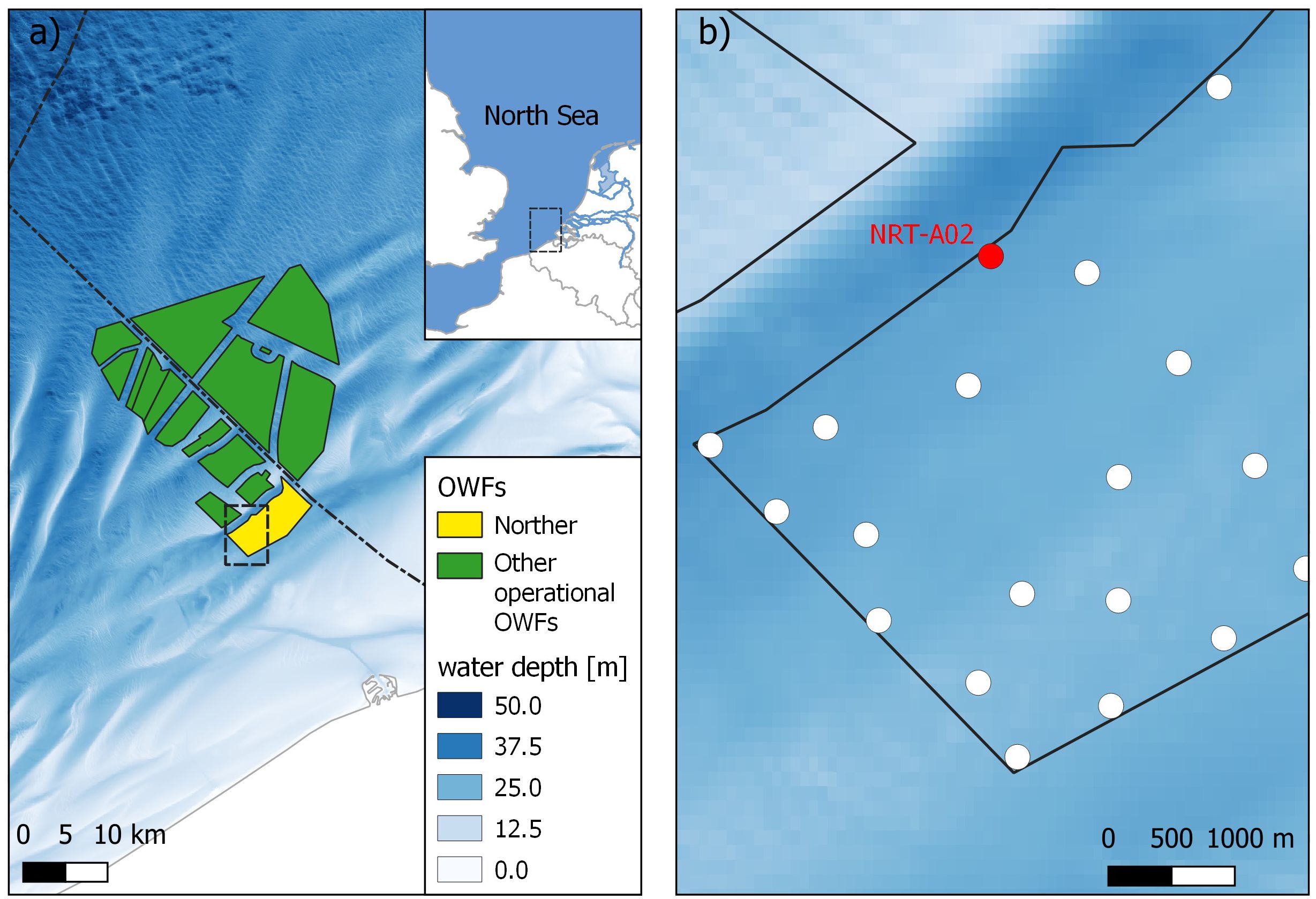
Figure 1. (a) Location of OWF Norther in the wind farm zone on the maritime border of Belgium and the Netherlands (border shown with dash-dotted line). Dashed line indicates area shown in (b). Water depths relative to LAT, as obtained from EMODnet (2022). (b) Location of monopile NRT-A02 within OWF Norther, as indicated by the red dot. Other monopiles in OWF Norther indicated with white dots.

Ivanov et al. (2020) provide a comprehensive overview of hydrodynamic conditions in this part of the North Sea, based on extensive modelling. In summer, temperature gradients over depth are generally smaller than 1°C. Similarly, salinity gradients are small at our study site as it does not seem to be affected substantially by either the Rhine or Scheldt river plume. Combined, this leads to a Potential Energy Anomaly (Simpson and Bowers, 1981) of less than 10 Jm^-3 in summer. In winter, PEA will even be lower due to frequent occurrence of storms and intense tidal currents (Ivanov et al., 2020).

Since 2012, multiple OWFs have been constructed in this area. We performed our measurements in OWF Norther, which is located southeast of the Thornton Bank at approximately 20–25 km offshore (Figure 1a). Within the OWF, water depths vary between 22 m and 30 m (Figure 1b), with reference to Lowest Astronomical Tide (LAT). The OWF was constructed in 2018 and 2019 and consists of 44 8.4 MW turbines. These are constructed on monopile foundations with a diameter of 7.8 m.

We conducted our measurements from 27-6–2022 until 30-6-2022, using the research vessel Simon Stevin from Flanders Marine Institute (VLIZ). The measurements focused on the hydrodynamics around a single monopile (NRT-A02, coordinates: 2.97084 E, 51.5262 N) (Figure 1b). This is relatively isolated, as the closest monopile is located 800 m to the east. Along the main tidal current axis, the closest monopiles are approximately 2 km away.

2.2 Experimental setup

We conducted different measurements around the selected monopile (Figure 2). In this section, we describe the methodology for each measurement separately. Postprocessing of the data is discussed in Sections 3.3-3.5.

Figure 2

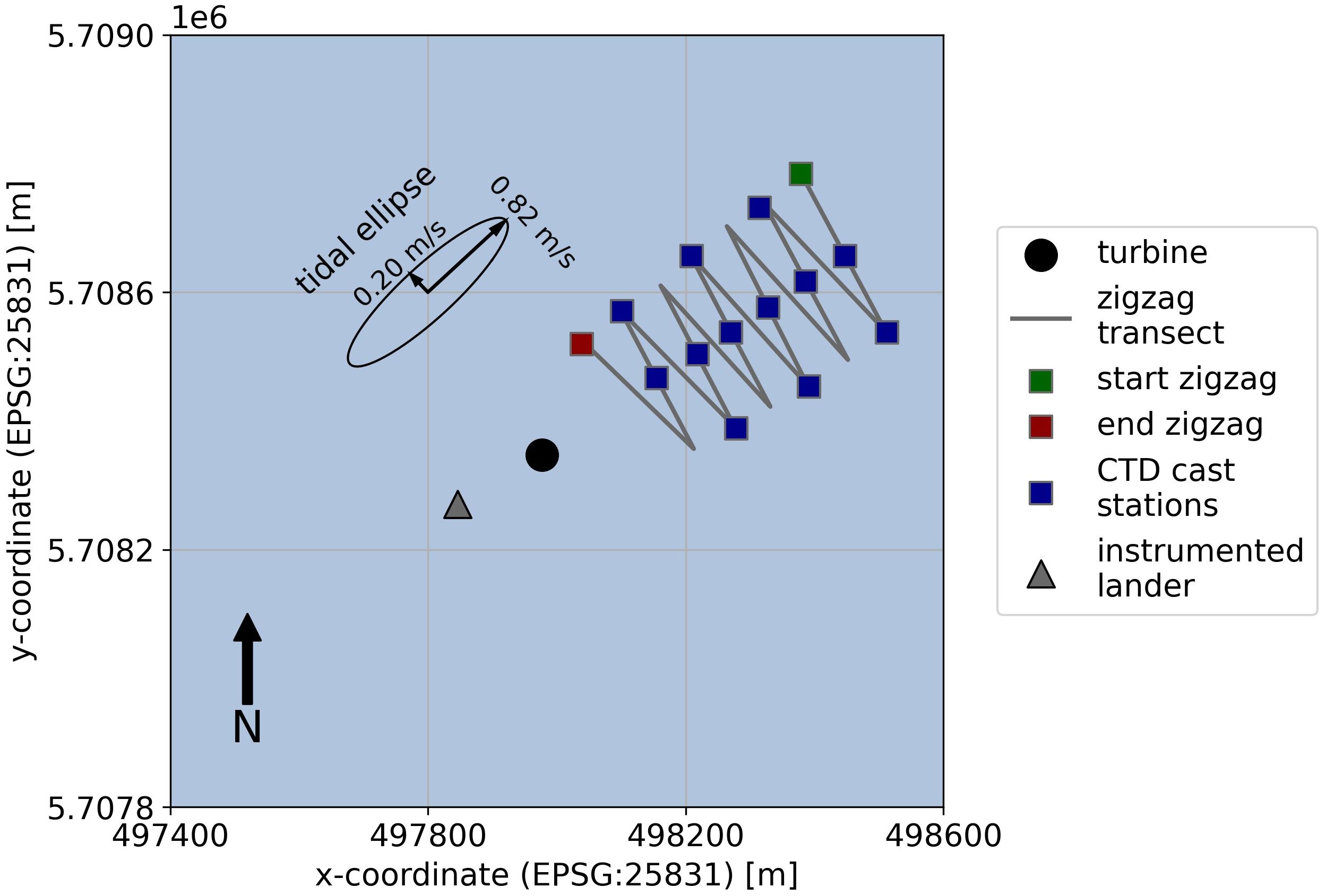
Figure 2. Layout of measurements around selected monopile. The tidal ellipse is drawn and labelled with the amplitude of the major and minor tidal axis.

2.2.1 Zigzag transect

Two identical zigzag transects were performed to determine the spatial extent of the monopile wake (Figure 2). Transects were sailed to the northeast of the monopile during peak flood (Figure 3), and their timing is listed in Table 1. The zigzag starting point was located 600 m away from the monopile. We gradually moved closer to the monopile by making 12 crossings, with the last crossing 180 m from the monopile. Each crossing was approximately 300 m long, and oriented almost perpendicular to the peak flood direction. Sailing speed was 2 to 3 knots.

Figure 3

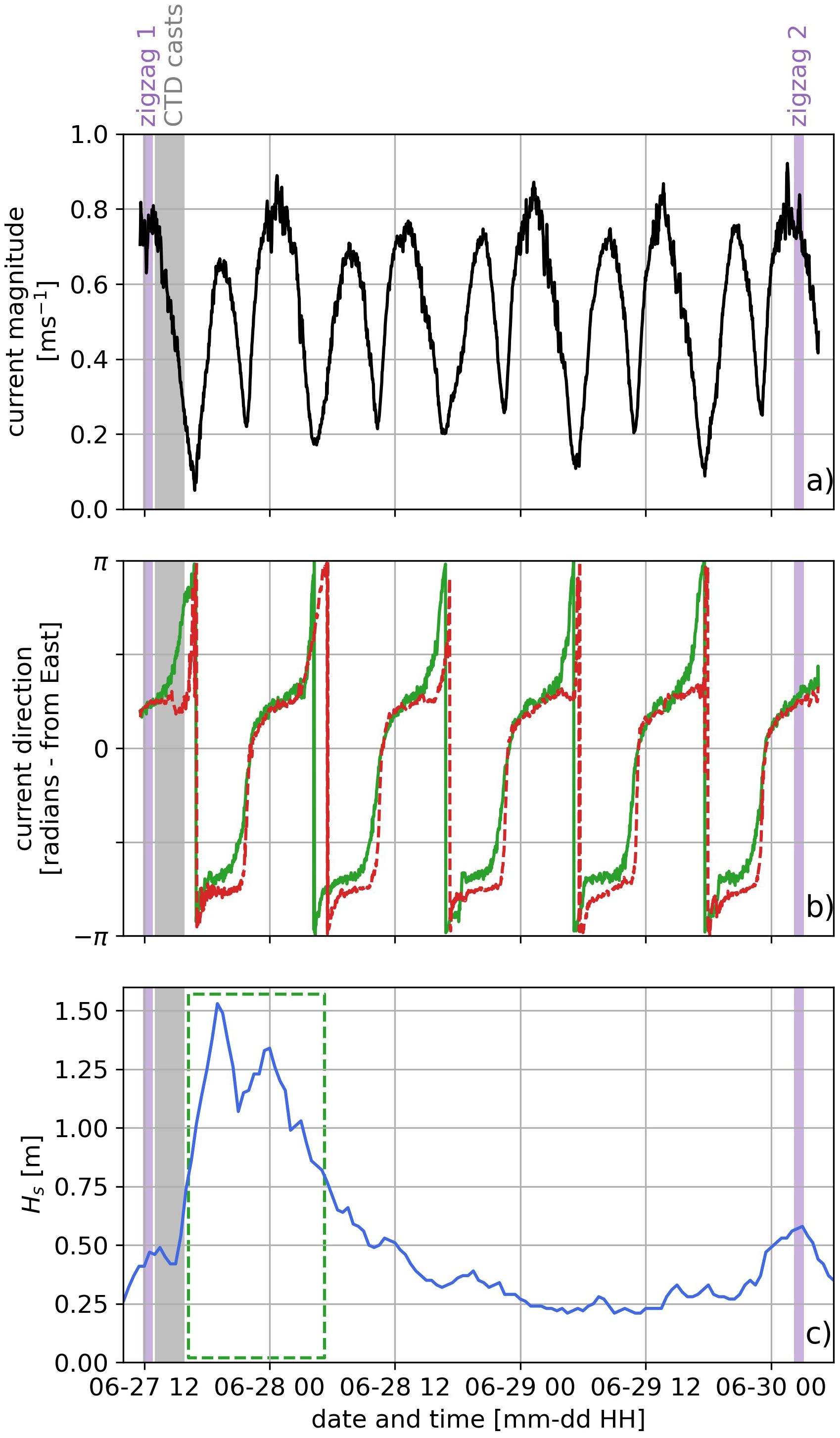
Figure 3. Hydrodynamic conditions during field campaign. Purple and grey hatches indicate timing of zigzag transects and CTD casts respectively. (a) Depth-averaged current magnitude from lander-mounted ADCP. (b) Current direction from lander-mounted ADCP. Dashed red line: near-surface direction (26 m above bed). Solid green line: near-bed direction (2 m above bed). (c) Significant wave height at Thornton Bank South Buoy. Green dashed box indicates wave-affected period.

Table 1

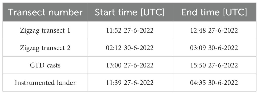
Table 1. Timing of actions during measurement campaign.

During each transect, salinity and temperature were measured at a 1 Hz frequency using the ship’s underway sensor lab. The water intake for this sensor lab is located near the bow, at a depth between 330 and 340 cm below the waterline. The water temperature is measured at the water intake using an SBE38 Oceanographic Thermometer, after which the water is pumped to the SBE21 thermosalinograph (TSG) near the aft of the ship. Subsequently, the water is discharged. The SBE 21 has an initial accuracy of ± 0.001 Sm^-1 for conductivity, and ± 0.01°C for temperature, with a resolution of ± 0.0001 Sm^-1 for conductivity, and ± 0.001°C for temperature. For the SBE38 initial accuracy is ± 0.001°C and resolution is ± 0.0003°C.

Flow velocities were measured via Teledyne RDI VM-DAS software using a vessel-mounted RDI Workhorse Mariner 600 kHz ADCP, in cells of 1 m. Navigation information was retrieved from vessel’s network and is based on the combination of a Septentrio RTK GNSS and a survey grade gyrocompass (Exail Octans Surface). During the first transect, the ADCP profiling interval was 10 seconds (i.e. 1 ping per 10 seconds). Preliminary analysis showed that this was insufficient for capturing the monopile wake. Hence, before the second transect took place, we changed the velocity profiling interval to 2 seconds. Only the velocity profiles collected during the second transect were analyzed.

2.2.2 CTD casts

After zigzag transect 1 was completed, CTD casts were taken at predefined locations along the zigzag transect (Figure 2 and Table 1). At each location, a down- and upcast were collected using a SBE21 rosette sampler. This CTD had the same resolution as the CTD mentioned in Section 3.2.1.

At the stations aligned with the peak flood direction, water samples were collected at 3 m above the seabed, mid-water column and 3 m below the surface. At each depth, water was collected using two 5L Niskin bottles mounted on the rosette sampler. Subsamples of 1 liter of water were filtered for Suspended Particulate Matter (SPM), and similarly, subsamples (0.3 – 0.58 liters of water) were filtered for POC and PON. Filtering was done using pre-weighed filters, which were stored at -18°C and transferred to the laboratory for further analysis.

2.2.3 Instrumented lander

At the beginning of the measurement campaign, an instrumented lander was deployed at the southwestern side of the monopile, at approximately 150 m distance from the monopile (Figure 3). This means it was located approximately 20 pile diameters from the monopile in ebb direction. It was retrieved at the end of the campaign (Table 1). Water depth at the lander location varied between 29 and 32 m.

The lander, a VLIZ multi-purpose mooring, consists of a custom stainless-steel frame with rope canister and acoustic release based on expertise from Goossens et al. (2020). For this study it was equipped with a CTD sensor, an upward-looking ADCP placed in a gimbal, and a seabed profiling sonar (Fourie et al., 2024). Here, we only discuss the CTD and ADCP data.

The CTD (RBR Concerto) measured at 1 Hz, and was mounted at 0.65 m above the seabed. It recorded from the start of the deployment until 30 June 00:50. This early termination was due to a sensor error. RBR Concerto has an initial accuracy of ± 0.003 Sm^-1 for conductivity, and ± 0.002°C for temperature, with a resolution of ± 0.0001 Sm^-1 for conductivity, and< 0.00005°C for temperature.

The ADCP (Nortek Signature1000) was located 1 m above the seabed. The ADCP was configured to measure in dual mode, measuring both averaged velocity profiles (1 Hz) and burst velocity profiles (4 Hz) in 1 m cells. Average velocity profiles were collected over the full water column, while the burst velocity profiles were limited to the lower 25 m of the water column. This was the maximum profiling range for the Signature in this mode.

2.3 Data processing zigzag transects

Both the salinity, temperature and velocity time series were converted to a location in ETRS89 UTM31N coordinates (EPSG: 25831) based on the ship’s position retrieved from its GNSS system.

2.3.1 Salinity and temperature of near-surface water

Temperature time series from the SBE38 thermometer at the water intake were used, while salinity time series were taken from the SBE21 TSG in the wet lab. The salinity time series had a time lag of 24 seconds and thus needed to be shifted. This time lag was detected by cross correlating the temperature time series from the SBE38 and SBE21. The time lag is caused by the time needed for pumping the seawater from the intake to the wet lab.

To extract timeseries for each transect, we used the start and end time of the zigzag transects (Table 1). These were both processed by an initial despiking using a three-minute rolling median (i.e., all values deviating more than 0.4 units (temperature and salinity) from the rolling median were removed) and a subsequent detrending using locally weighted scatter plot smoothing (LOWESS). LOWESS regression was required, as sea surface temperature (SST) during transect 1 increased by a similar order of magnitude as the wake-induced effect. To be consistent, we applied the LOWESS regression for both transects and for both temperature and salinity.

For the temperature time series of transect 1 and 2, and the salinity timeseries of transect 2, we performed a one-step regression. The timeframe for the LOWESS regression was set to 5 minutes, corresponding to the time required for sailing a single transect line. For the salinity time series of transect 1, a two-step LOWESS regression was required due to measurement noise. Firstly, a 5-minute window LOWESS regression was fitted to the data. Secondly, we took the detrended data and fitted a 1-minute LOWESS regression to the data, which corresponds to the approximate wake width for these monopiles.

2.3.2 Vessel-mounted ADCP velocity profiles

The data from the vessel-mounted ADCP was postprocessed using the CODAS toolbox (Hummon, 2009). This toolbox consists of a set of routines for quality control and processing of RDI ADCP data as acquired by VM-DAS. Velocity data were corrected for pitch, roll and heave of the vessel. No heading correction nor calibration needed to be applied to the data. The quality-controlled data were then ensemble averaged with an ensemble time of 10 seconds, thus including 5 profiles per ensemble. Processed data were stored in standardized netCDF format.

2.4 Data processing CTD casts

The CTD cast data were postprocessed using both SeaBird SBE data processing software and Python. The SeaBird software was used for deriving salinity from conductivity, pressure and temperature using EOS-80 formulations.

These data were then read and processed using the Python toolbox python-ctd (Fernandes, 2025). First, up- and downcasts were separated. Readings below 4 dbar or where a pressure sign reversal occurs were removed. The data was then despiked and missing values were interpolated linearly. Finally, the pressure in dbar was converted to depth below the surface and data was binned in 0.1m cells.

Water density was derived from salinity, temperature and depth following EOS-80 formulations. We then computed the Potential Energy Anomaly (PEA, symbol: $\varphi$) to quantify stratification strength for each profile, according to Simpson et al. (1994):

$$\varphi =\frac{1}{h}{\displaystyle {\int }_{-h}^0(\widehat{\rho }-\rho )gz \text{dz}}; \widehat{\rho }=\frac{1}{h}{\displaystyle {\int }_{-h}^0\rho \text{dz}}$$

Where ρ (z) is the density over the water column at depth h. $\varphi$ [Jm^-3] is the amount of work required to achieve complete mixing of the water column.

2.5 Data processing instrumented lander

2.5.1 Lander CTD

The lander CTD data were resampled to a 5 second interval and missing values in the dataset were linearly interpolated. Water density was derived from salinity, temperature and depth following EOS-80 formulations. The timeseries were then linearly detrended for the full deployment period.

2.5.2 Velocity profiles and turbulence

From the ADCP data, we utilized both the average velocity profiles and the high-frequency velocity profiles. The former were taken as direct output from the Nortek processing software, while the latter were processed using the ‘5-Beam-Turbulence-Methods’ toolbox (Guerra and Thomson, 2017).

Using this toolbox, the high-frequency data were quality controlled and outliers removed. The data were divided into 10-minute bins to compute turbulence characteristics. Then, the turbulent kinetic energy (TKE [m²s^-2]) was computed by separating the velocities in all three directions (u, v, w) in an average and fluctuating part:

$$u= \overline{u}+u^{\prime }; v= \overline{v}+v^{\prime }; w= \overline{w}+w^{\prime }$$

$$TKE=0.5(u^{\text{'}2}+v^{\text{'}2}+w^{\text{'}2})$$

TKE is then depth-averaged as we want to quantify the total amount of additional mixing brought about by the monopile.

The turbulent kinetic energy spectra were also computed, but we could not derive a reliable estimate for the turbulent energy dissipation (ϵ) due to the presence of waves in the frequency domain.

2.6 Additionally utilized data

Significant wave heights and periods measured at the nearby Thornton Bank South wave buoy (Datawell – directional waverider) were downloaded from the Flemish Banks Monitoring Network (Meetnet Vlaamse Banken, 2024). The wave buoy is located 4 km from the monopile (location: 2.98667 E – 51.56472 N). Additionally, we utilized SST data measured at this wave buoy for verifying our near-bed CTD measurements and transects.

3 Results

3.1 Hydrodynamic conditions during the field campaign

Hydrodynamic conditions during the field campaign are characterized by a strong flood-dominant tide (Figure 3a). Maximum depth-averaged currents during flood reach up to 0.8 – 0.9 ms^-1, while during ebb, they reach up to 0.6 – 0.7 ms^-1 (Figure 3a). Currents are mainly oriented northeast (flood) to southwest (ebb) (Figure 3b). During flood, the near-bed current direction (Figure 3b – solid green line) is well-aligned with the near-surface direction (Figure 3b – dashed red line). During flow reversal from flood to ebb, the near-surface direction lags behind the near-bed direction, with a time lag of approximately 30 minutes. Some vertical shearing seems to take place during ebb, with the near-bed direction directed somewhat more in southerly direction than near-surface direction.

Both zigzag transects took place during peak flood conditions (purple hatches - Figure 3), when currents were directed in north-easterly direction. The CTD casts were still taken during flood (gray hatch - Figure 3), though the current was already rotating to a more northerly direction throughout most of the water column (Figure 3b).

Significant wave heights (H_s) were generally low throughout the campaign, apart from the evening of June 27 until the morning of June 28 (Figure 3c). Significant wave heights start increasing at the end of the afternoon, peaking at about 1.5 m around June 27 20:00. Afterwards, significant wave heights decrease slowly to less than 0.5 m the following morning. For the timeseries analysis, we define the period when significant wave heights exceed 0.8 m as the ‘wave-affected’ period, as this is the 50^th wave height percentile at this location in 2022. However, these conditions are still relatively mild for the southern North Sea.

3.2 Near-surface salinity and temperature show wake extent

The zigzag transects reveal a clear influence of the monopile wake on near-surface temperature and salinity (Figure 4). During the first transect, a 70-m to 100-m wide band of cooler and more saline water extends in the flood direction downstream of the monopile. The water is up to 0.2 °C colder and salinity 0.25 higher than its direct environment. More than 400 meters downstream of the monopile, the temperature and salinity differences become less pronounced.

Figure 4

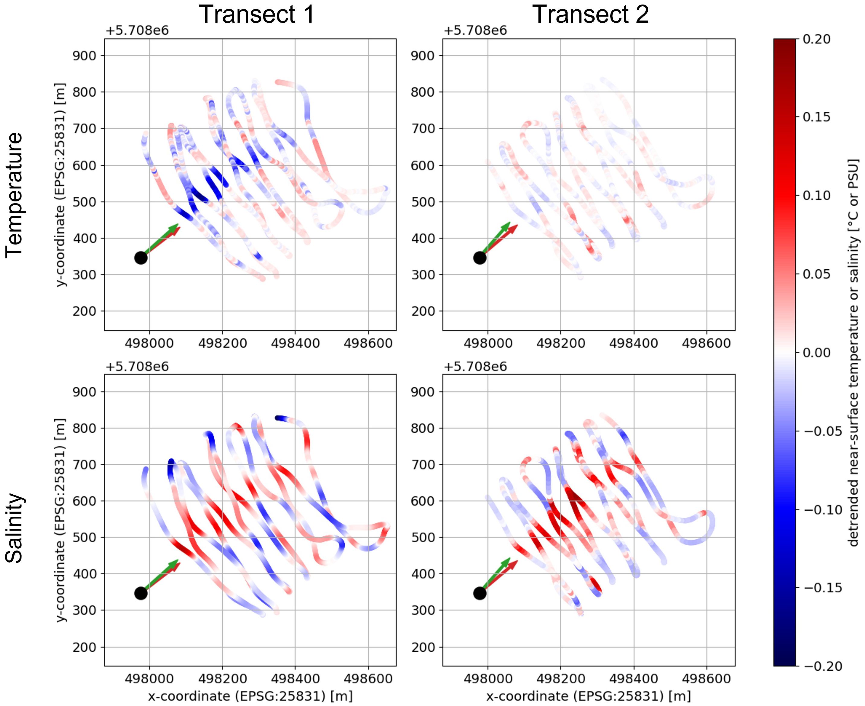
Figure 4. Detrended near-surface temperature and salinity during zigzag transect 1 and 2. The results for the first transect are shown in the left panels, while the right panels show the second transect. Each dot indicates the vessel position during this transect on a 1Hz frequency, and is colored according to its detrended temperature or salinity. The large black dot indicates the monopile location. The red and green arrows show the tidal current direction at the start and end of each transect, respectively.

During the second transect, we observe again more saline water downstream of the monopile. This is found along the same 70 to 100 m wide band as during the first transect. The difference in salinity between the monopile-affected area and environment is comparable to the first transect, with salinity differences of up to 0.25. We did not observe any substantial near-surface temperature differences during the second transect, which is likely due to timing of the sailed transect (Table 1). As this was at the end of the night (local time), there had not been solar input for at least 7 to 8 hours prior to the transect.

During both transects, the wake could not be observed visually. Previous studies (e.g. Bailey et al., 2024) report observations of a turbid wake downstream of monopiles. This could not be observed at our study site, likely due to the low SPM concentrations throughout the campaign.

3.3 Vertical salinity and temperature profiles become more well-mixed

The CTD casts show the vertical salinity and temperature profiles generally show a well-mixed to weakly stratified water column. This is quantified through the PEA, shown in Figures 5a, c. The PEA varies between 2.3 and 6.9 Jm^-3. The lowest PEA values are found close to the turbine, less than 200 m away, when the tidal current is aligned with the station location.

Figure 5

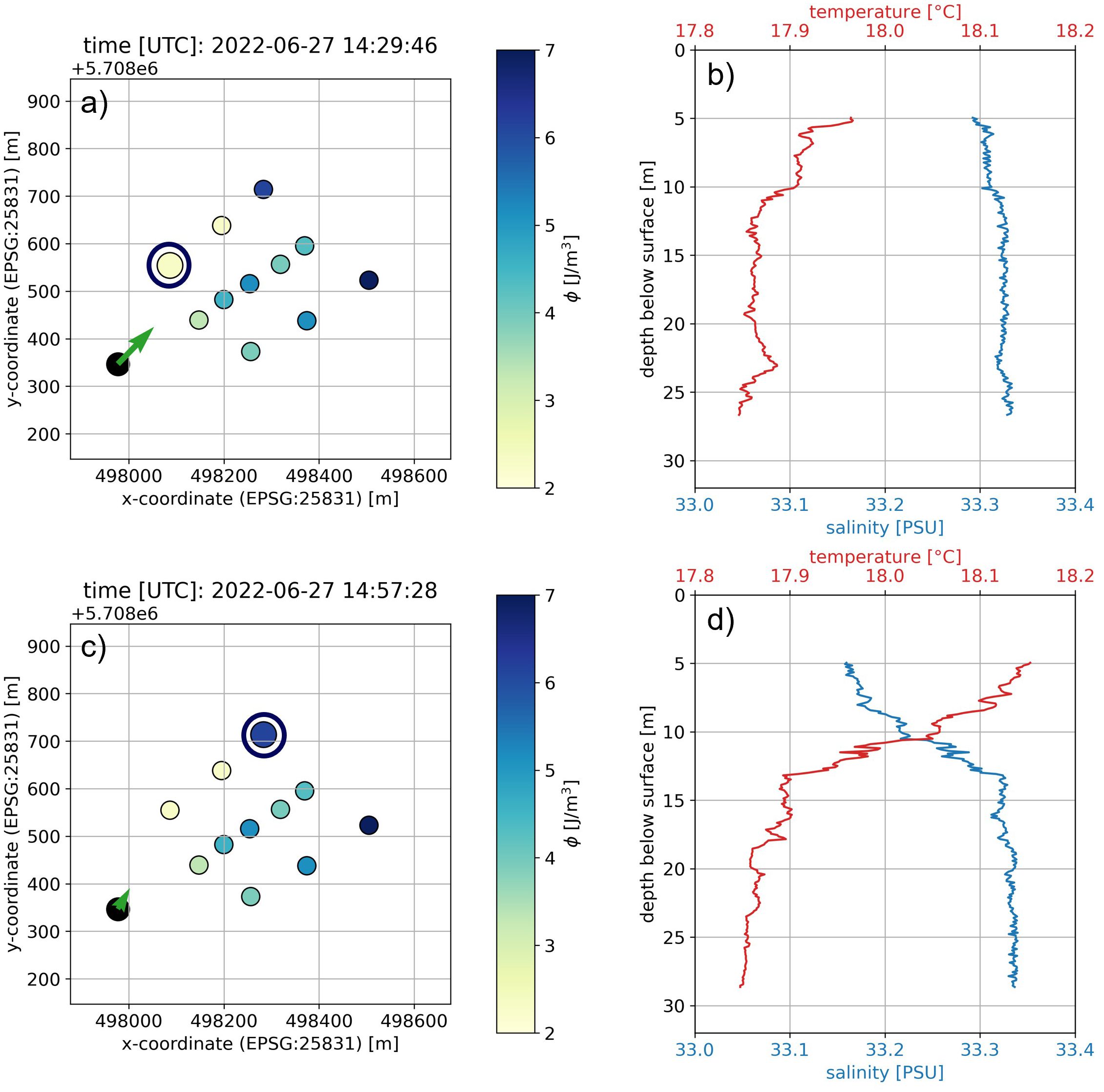
Figure 5. Overview of CTD casts collected directly after zigzag transect 1. (a, c) Overview of CTD stations and computed PEA for each station. Encircled cast was taken at time in subplot title. Green arrow indicates depth-averaged tidal current direction at this time. (b, d) Vertical profiles of temperature and salinity for stations encircled in (a, c), respectively.

To further illustrate the difference between the monopile-affected vertical profiles and the others, representative vertical profiles of salinity and temperature are shown in Figures 5b, d for the two stations encircled in Figures 5a, c. Closest measurements to the monopile show an almost entirely mixed water column (Figure 5b). When the tidal current is not aligned with the station location, the PEA increases. Highest PEA values are found at the two stations almost 600 m away from the monopile, showing a weakly stratified water column (Figure 5d).

The temperature at 5m below the surface is approximately 0.15°C lower for the monopile-affected stations, and salinity is almost 0.15 PSU higher (Figures 5b, d). These values are consistent with the near-surface measurements of zigzag transect 1 (Figure 4).

3.4 Temporal wake effect from near-bed salinity and temperature

The lander-mounted CTD showed near-bed salinity and temperature vary mostly on a semidiurnal basis. The highest near-bed salinities and lowest temperatures occurred during peak flood (Figures 3, 6). Vice versa, lowest salinity and highest temperature were observed during peak ebb. Salinity sharply decreased and remained constant during the wave-affected period on 27 June until it resumed its diurnal variation on June 28. Temperature steadily decreased on June 27 and remained more or less constant until June 28 12:00. Afterwards, it also resumed its diurnal variation. The third pattern in the timeseries are the three peaks occurring on June 28 and 29. As these are likely caused by the monopile wake, we will discuss these in more detail below.

Figure 6

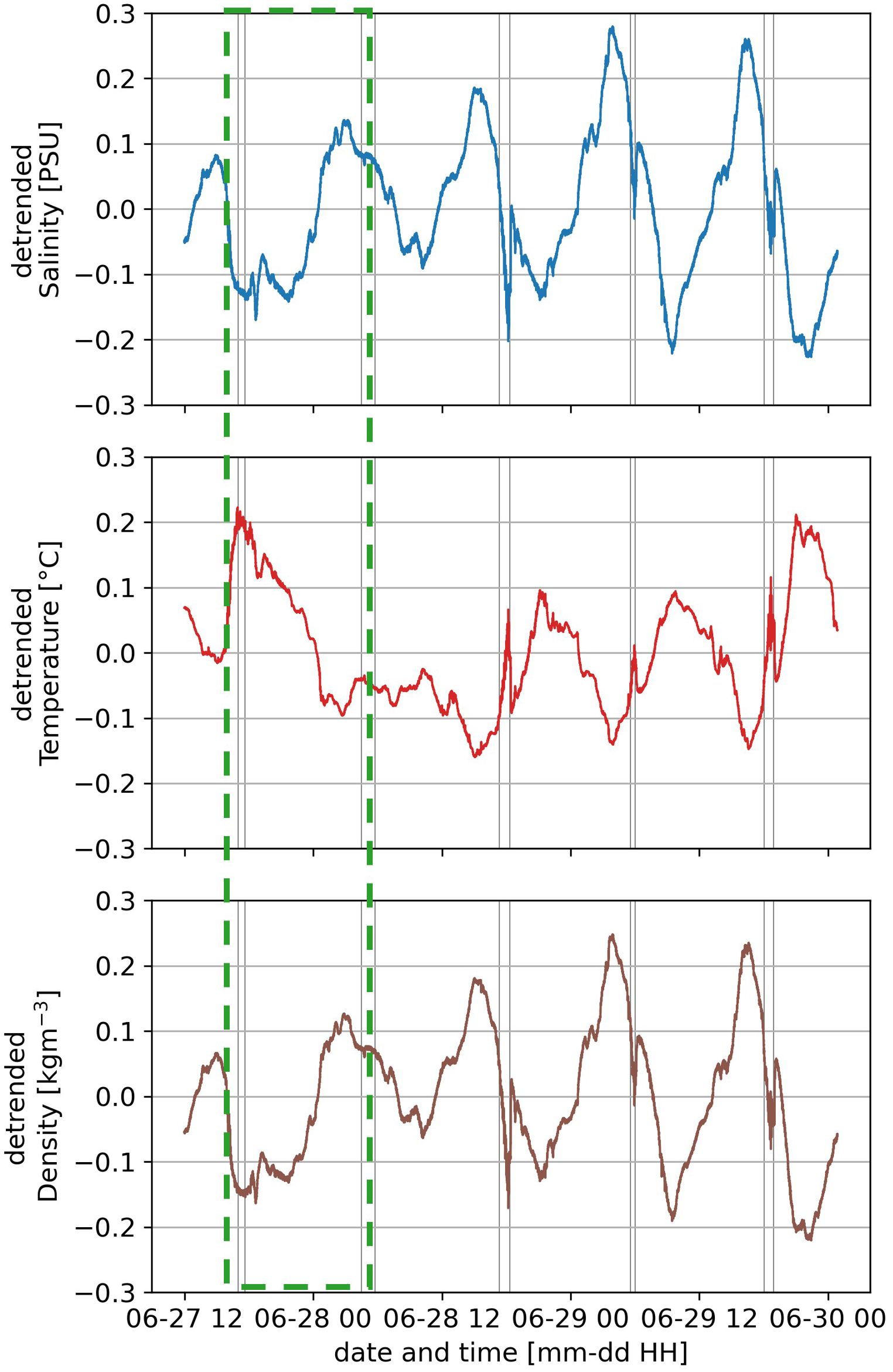
Figure 6. Detrended salinity, temperature and density timeseries from the CTD on the instrumented lander. Grey boxes indicate when the lander is in the near-bed monopile wake. Green dashed area indicates the wave-affected period.

The three peaks show a simultaneous response in salinity and temperature (Figure 6 upper and middle panel) and occur during the early ebb phase, when the lander is downstream of the monopile. Salinity decreases down by<0.2 PSU compared to its regular semidiurnal variation, while temperature increases by<0.2°C.

To determine whether these peaks are caused by the monopile wake, we analyzed the tidal current direction during the early ebb phase. Since there is a substantial difference in direction between the near-bed and near-surface current (Figure 3b), we considered current direction at three heights: near-surface, mid-water and near-bed, as measured by the lander-mounted ADCP. We then analyzed the monopile wake direction at each height, assuming a wake width of ten times the monopile diameter (Rogan et al., 2016; Schultze et al., 2017; Dorrell et al., 2022). A period is considered monopile-affected when the wake, plotted along the current direction, aligns with the lander position relative to the monopile, hereafter called ‘lander direction’.

The peaks in salinity and temperature occur when the near-bed wake aligns with the lander direction. This period is indicated with the grey hatches in Figure 6. Once the near-bed current starts to align with the lander direction, the salinity sharply decreases and temperature sharply increases. Within minutes after the near-bed current has rotated beyond the lander direction, both temperature and salinity resume their semidiurnal variation.

The temporary increase in temperature and simultaneous decrease in salinity are consistent with the near-surface measurements and vertical profiles. They all imply increased mixing due to the monopile wake.

3.5 Velocity decrease in upper part of the water column

During the second zigzag transect, the depth-averaged flow velocity magnitude at the lander, upstream of the monopile, varied between 0.7 to 0.8 ms^-1 and was directed predominantly in northeasterly direction (Figures 3a, b). Depth-averaged flow velocity magnitude and direction along the transect, downstream of the monopile, agree well with these observations. In Figure 7, we show the ensemble-averaged velocities for the near-surface (Figure 7a) and near-bed layer (Figure 7b), as measured by the ship’s ADCP.

Figure 7

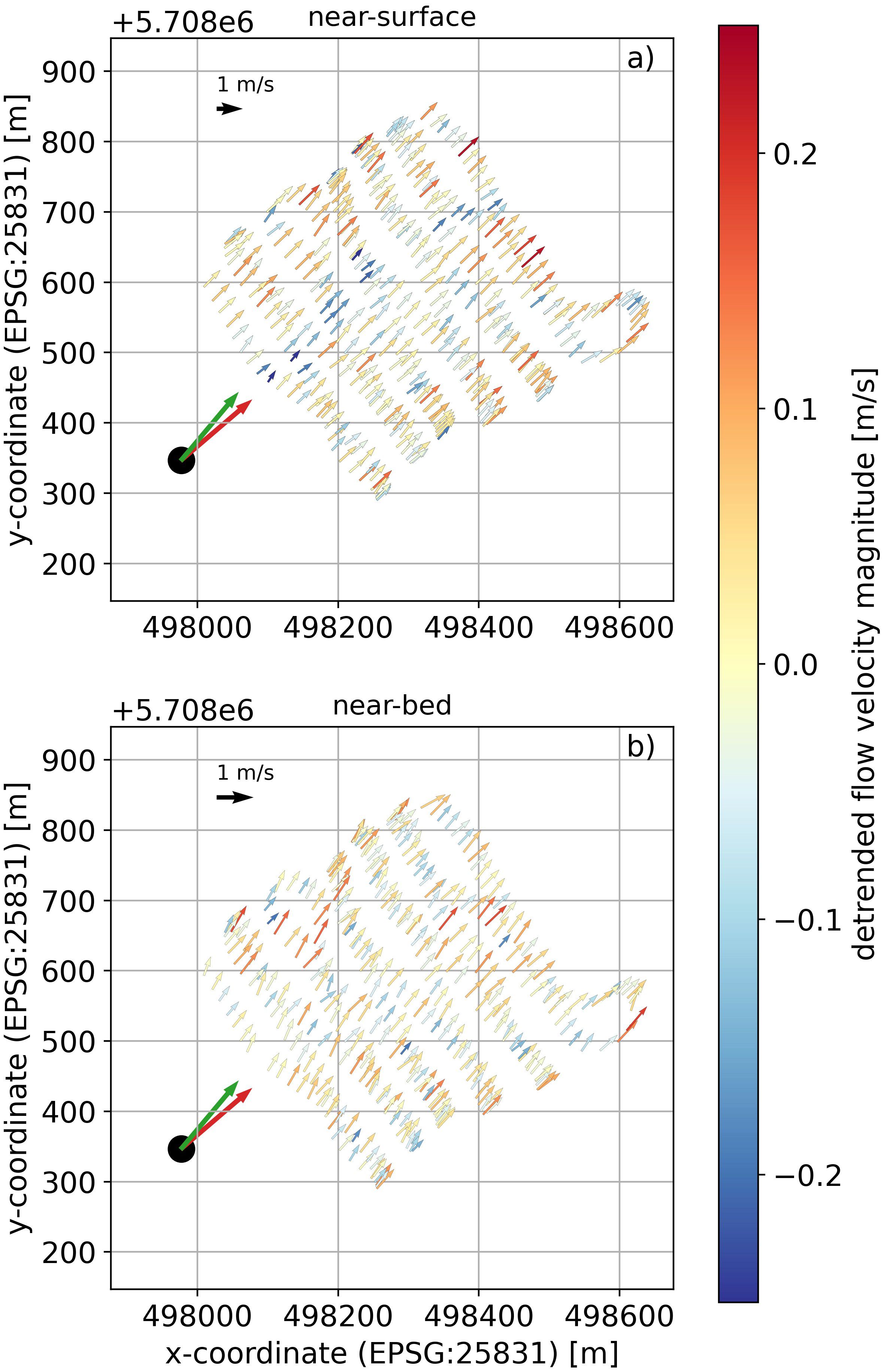
Figure 7. (a) Near-surface and (b) near-bed flow velocity during zigzag transect 2. Here, near-surface corresponds to 5 m below the surface and near-bed to 2 m above the bed. Arrows along the transect indicate the velocity magnitude and direction of an ensemble and are located at the ensemble midpoint. Arrow colors are based on the LOWESS-detrended (Section 3.3.1) flow velocity. Note the difference in arrow scale between subplots. Similar to Figure 3, the monopile position is indicated with the black dot and tidal current direction is shown by the red and green arrows, which are not scaled.

Near the surface (Figure 7a), the flow velocity magnitude downstream of the monopile decreases by up to 0.2 ms^-1 compared to its direct environment. This is most pronounced within 350 meters downstream, with a reduction of up to 25% in flow velocity magnitude within the monopile wake. Beyond this distance, the velocity difference between the wake and its environment cannot be distinguished from the regular variation between ensembles.

Over the water column, flow velocity magnitude steadily decreases, until it reaches a minimum near the bed (Figure 7b). Similarly, velocity magnitude differences between the wake and its environment steadily decrease. Until 15 m below the surface, a velocity magnitude decrease can be observed within the wake. Near the bed (Figure 7b), the wake cannot be determined from these velocity measurements.

3.6 TKE increases in the wake

In this section, we compare TKE inside the wake to outside the wake. As TKE is computed from the lander-mounted ADCP timeseries (Section 3.5.2), we need to determine which 10-minute subsets of this timeseries should be classified as ‘inside wake’ or ‘outside wake’. Hereto, we followed a similar approach as in Section 4.4.

We categorized a 10-minute bin as monopile-affected when the wake plotted along the depth-averaged velocity direction overlapped with the lander direction. Though there is a considerable difference in direction between the near-bed and near-surface direction (Figure 3b and Section 4.4) during the early ebb phase, using the depth-averaged direction seems most appropriate as the other considered variables are also depth-averaged. After categorizing the ‘inside wake’ and ‘outside wake’ subsets, we separated these points from the wave-affected subset (Figure 3c). Finally, we only considered 10-minute bins where the depth-averaged velocity magnitude falls between 0.25 and 0.55 ms^-1, as this was the velocity range encountered during the ‘inside wake’ subset.

Figure 8 shows the depth-averaged TKE as a function of depth-averaged velocity (U) for three distinct subsets: outside the wake (gray), inside the wake (orange) or wave-affected (green). Depth-averaged TKE is lowest for the ‘outside wake’ subset, ranging from 1·10–³ to 2·10–³ m²s^-2. For the ‘inside wake’ subset, this range increases considerably. While the lowest wake-affected TKE values are in the order of 1.5 10–³ m²s^-2, they may increase up to 5 10–³ m²s^-2. The wave-affected TKE is considerably higher than the TKE within the wake, leading to a range in TKE from 3·10–³ to 1·10–² m²s^-2.

Figure 8

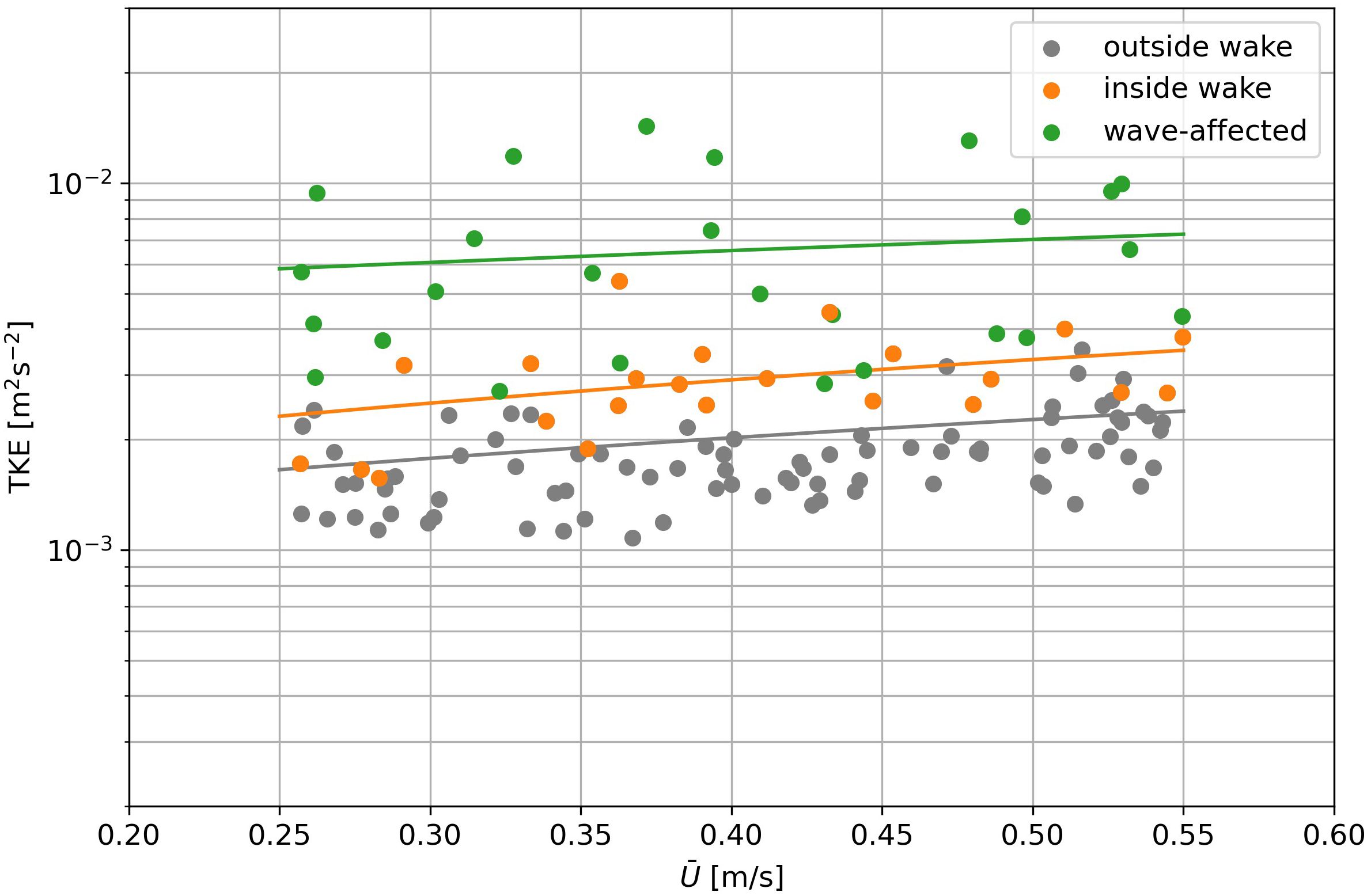
Figure 8. TKE as a function of depth-averaged flow velocity (U). We consider three different periods: outside the wake (gray), inside the wake (orange) and wave-affected (green). Each point corresponds to a 10-minute bin. Solid lines are linear regressions for each subset.

The linear regression for each subset confirms that TKE is higher inside the wake than outside the wake. All subsets show the best correlation with a linear regression, though we would expect a quadratic relationship between the depth-averaged velocity (U) and depth-averaged TKE (Calvino et al., 2023). For the wave-affected subset, the slope of the linear regression is fairly small. Likely, the waves dominate depth-averaged TKE during this period, with the tidal current only playing a minor role.

4 Discussion

4.1 Wake dimensions and hydrodynamic impact

The synoptic measurements presented in the previous section allow the characteristics of the monopile-induced wake to be understood. As the monopile is relatively isolated, hydrodynamic wakes from other monopiles are unlikely to have interfered with our measurements. We relate the wake dimensions to the monopile diameter, as previous research has shown that this is the relevant scaling parameter (Rogan et al., 2016; Schultze et al., 2020a; Dorrell et al., 2022).

Our measurements show that the monopile wake is relatively confined in both space and time. The zigzag transects show a sharp interface between the wake-affected area and its environment, for both near-surface salinity and temperature (Figure 4). This is corroborated by the swift response of the near-bed salinity and temperature to the wake presence (Figure 6). The wake has a width of approximately 70 meters, which is about 10 times the monopile diameter. This is consistent with previous estimates (Rogan et al., 2016; Schultze et al., 2020a; Dorrell et al., 2022).

Most pronounced effects on near-surface temperature, salinity and velocity are observed within 350 to 400 m from the monopile (Figures 4, 7). This suggests a wake length of 50 to 60 times the monopile diameter, similar to Schultze et al. (2020b). Other wake length estimates are considerably higher (e.g., Li et al., 2014; Forster, 2018) as these studies estimate wake dimensions from the turbid plumes observed downstream of monopiles. We will discuss this difference in more detail in Section 5.2.

We quantified the increase in turbulent mixing within the wake by computing the depth-averaged TKE (Figure 8) at the lander. The TKE within the wake is 35 to 50% higher than outside the wake. Rogan et al. (2016) estimated from laboratory experiments that the increase in TKE at 20 pile diameters from a monopile would be 100% compared to undisturbed turbulent flow. Thus, our measured effect is not as pronounced as in the laboratory experiments of Rogan et al. (2016), though it is still in the same order of magnitude.

Apart from the increase in TKE, previous modelling studies also suggest a local decrease in flow velocity due to the monopile wake (Grashorn and Stanev, 2016; Cazenave et al., 2016; Rivier et al., 2016; Schultze et al., 2020a). These effects diminish with downstream distance from the monopile, as most pronounced differences with the environment occur within 10 to 20 pile diameters. The closest point of our zigzag transect lies roughly 21 pile diameters from the monopile in flood direction, so already beyond this range. Still, the velocity decrease is clearly visible in the near-surface velocity field (Figure 7a). However, more than 15 m below the surface it was not observed anymore (Figure 7b).

It is not clear why this velocity decrease varies with depth. One explanation is the general decrease in velocity magnitude with depth, which makes a proportional velocity decrease harder to detect. Another possibility is a more pronounced wake near the surface because of a higher surface roughness of the monopile in the upper part of the water column compared to the lower sections. The intertidal part is generally colonized by relatively thin layers of barnacles and flexible macroalgae (Degraer et al., 2020). The fauna in the upper subtidal belt is dominated by blue mussels (Mytilus edulis) occurring in high densities (1843 ind. m-2 in the nearby C-Power wind farm, Mavraki et al., 2020) These are relatively large and their hard shells contribute to a substantial surface roughness. This roughness is known to change wake characteristics (e.g. Achenbach and Heineke, 1984). Deeper down, the fauna is dominated by flexible mats of small amphipods (Jassa herdmani) while near the sea floor the communities are dominated by soft anemone species (Degraer et al., 2020). So, monopile roughness will likely vary with depth. This may be further enhanced by monopile design and the presence of auxiliary infrastructure on the monopile, such as cathodic protectors. In general, the velocity decrease with depth is likely to be a combined effect of both the ambient velocity profile over depth and increased near-surface roughness.

4.2 Changes in vertical gradients of salinity, temperature and suspended matter

Within the wake, near-surface salinity increased and water temperature decreased (Figure 4). Near the bed, salinity decreased and temperature increased within the wake (Figure 6). Though the near-surface and near-bed measurements were not collected simultaneously, they are consistent with one another. These measurements are corroborated by the vertical profiles of temperature and salinity (Figure 5). When affected by the monopile wake, the weakly stratified water column was almost entirely mixed (Figure 5b). The decrease in stratification, as quantified through the PEA (Section 4.3), is consistent with the 65% decrease in PEA reported by Dorrell et al. (2022) (based on Schultze et al., 2020a).

The decrease in the vertical density gradient can be explained by the monopile-induced increase in turbulent mixing (Figure 8). When turbulent mixing increases, the temperature and salinity difference between the near-surface and near-bed layer decreases (Figure 9 – left and middle panel). In periodically or seasonally stratified systems, this mixing may be inhibited by the presence of a pycnocline (Dorrell et al., 2022). In case of the BCZ, density differences over the water column are small, thus there is no pycnocline. Hence, the change in near-bed salinity and temperature is remarkably similar to the near-surface observations.

Figure 9

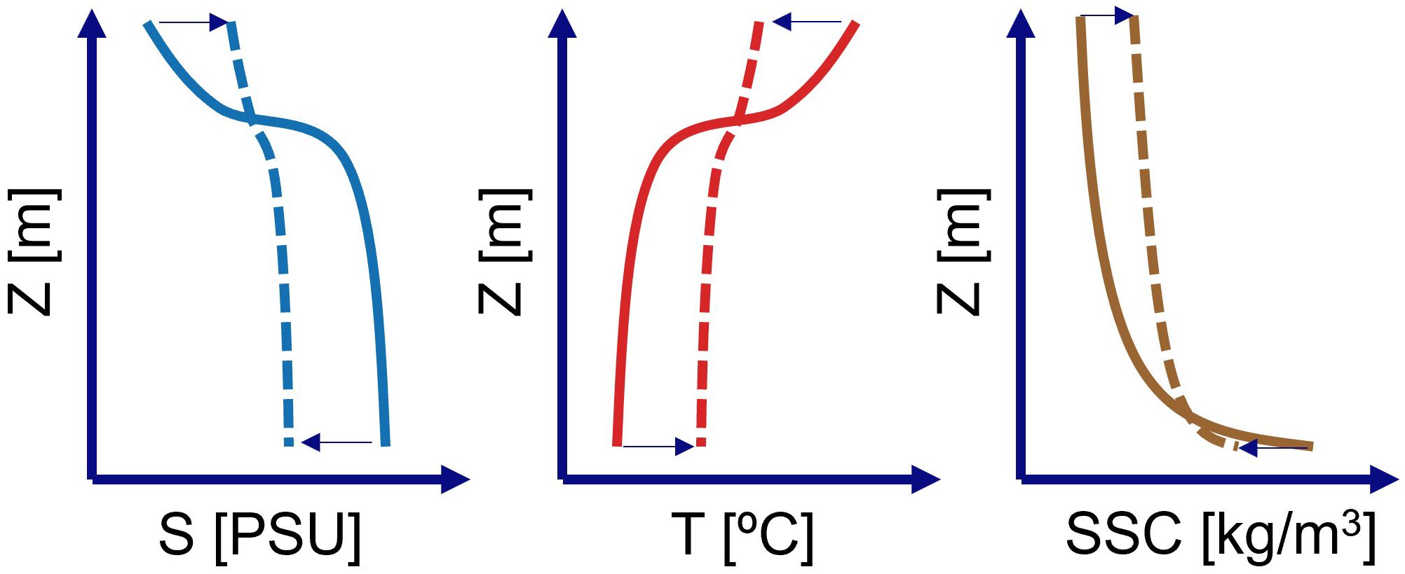
Figure 9. Conceptual sketch showing how salinity, temperature and SSC change over depth due to the monopile-induced increase in turbulent mixing. Solid line indicates undisturbed profile, while dashed line indicates monopile-affected vertical profile. Arrows at near-surface and near-bed indicate the monopile-induced effect observed in Section 4 (salinity and temperature) and hypothesized effect on SSC.

Apart from the wake-induced effects on temperature, we also observed a diurnal variation in water temperature. During the second zig-zag transect, there was virtually no difference in near-surface temperature inside and outside the wake (Figure 4). Similarly, the wake-induced temperature decrease in the CTD lander timeseries (Figure 6) in the early morning of June 29 seems less pronounced than the decrease during the afternoon of both June 28 and 29. Our findings are corroborated by the SST measured at the Thornton Bank wave buoy (Section 3.6), as these data show a diurnal variation in SST in the order of 0.3 to 0.6°C during our measurement period. This suggests that warming and cooling of the water column happens on a diurnal timescale, which is much shorter than in other parts of the North Sea, such as the German Bight and the northern North Sea (Van Leeuwen et al., 2015; Carpenter et al., 2016; Floeter et al., 2017).

The increased turbulent mixing may also have a pronounced effect on the vertical suspended sediment concentration (SSC) profile (Figure 9 – right panel). When the turbulent mixing increases, SSC gradients over depth become smaller. This leads to lower near-bed SSC while near-surface SSC increases. Even when there is no monopile-induced erosion from the seabed, this redistribution of suspended matter may lead to an increased near-surface turbidity. This likely causes the turbid plumes observed for multiple OWFs in the southern North Sea (e.g. Vanhellemont and Ruddick, 2014). Once the suspended matter is mixed to near-surface water layers, its low settling velocity (Van Maren et al., 2020) may lead to pronounced residence times higher up in the water column. As the suspended matter is advected downstream of the monopile near the surface, this may explain the long turbid plumes downstream of OWFs. A similar explanation discussing the origin of these turbid plumes was recently put forward by Bailey et al. (2024). This would mean that previous estimates of wake length based on remotely sensed turbidity (e.g., Li et al., 2014; Forster, 2018) should be treated with caution as they do not necessarily reflect the actual hydrodynamic wake, but rather the advection of suspended matter. Still, both wakes need to be considered as they may have their own effect on ecosystem functioning. For instance, advection of SPM in the upper reaches of the water column may still lead to a change in underwater light climate even if it is not strictly in the hydrodynamic wake. On the other hand, mixing of nutrients and passive substances will primarily take place in the hydrodynamic wake itself, closer to the monopiles.

4.3 Comparing monopile-induced mixing to other sources of mixing

The substantial increase in TKE during the wave-affected period (Figure 8) and the associated increase in turbulent mixing (Figure 6) raises the question how the different sources of turbulent production (P) compare to one another. These sources are either wind- and wave-induced (for simplicity signified by P_wave), structure-induced (P_D) or current-induced (P_B).

To put these into context, we need to consider three things. Firstly, TKE was measured close to the monopile (Figure 2). Secondly, waves and wind affect the entire area, while the wake is relatively confined in space (Section 5.1). And finally, the wave buoy data (Section 3.6) show that wave heights during the wave-affected period were still quite moderate for the southern North Sea, as the maximum observed wave height was exceeded by higher waves for 17% of the time in 2022.

We have not measured turbulent dissipation (ϵ), which is often used as a proxy for P (e.g., Carpenter et al., 2016; Schultze et al., 2017; Dorrell et al., 2022). However, if we assume total TKE (Figure 8) is proportional to the turbulent production and P_wave and P_B are both spatially uniform, we can estimate how these terms compare. If these assumptions are valid, P_wave would be 2 to 2.5 times larger than P_B. This is substantially lower than the ninefold increase in turbulent dissipation observed by Schultze et al. (2017) during the remnant of a tropical storm. This confirms that the wave-affected period in our observations was indeed a moderately energetic event.

Based on data of Scannell et al. (2021); Dorrell et al. (2022) computed a P_D of approximately 1.5 times P_B for the seasonally stratified Celtic Sea. As both terms scale with the cubed current velocity, this ratio could theoretically also apply to the southern North Sea. So, observed TKE inside the wake (Figure 8) would underestimate P_D. This is mainly due to the fact that turbulence production primarily takes place within 10–20 diameters downstream of the monopile (Schultze et al., 2020a).

So, we can conclude that when a storm takes place, P_storm will likely dominate both P_D and P_B. However, the permanent additional mixing induced by monopiles can have substantial effects, especially during fair weather periods.

4.4 Further implications of changes in stratification

In the previous sections, we have shown how an offshore wind turbine foundation affects local hydrodynamics and stratification. In this section we discuss how these findings contribute to assessing ecosystem impact of large-scale development of OWFs in the southern North Sea.

Monopile-induced mixing may lead to destratification in parts of the southern North Sea (Christiansen et al., 2023), especially when future offshore wind scenarios are considered (Van Duren et al., 2021 and Zijl et al., 2021). If this leads to destratification, this may multiple knock-on effects on the ecosystem. When present, the pycnocline forms a barrier for the vertical exchange of algae, nutrients, suspended matter and dissolved oxygen (Van Leeuwen et al., 2015; Boon et al., 2018). If the pycnocline is broken up, this affects primary production, though this effect is not uniform throughout the North Sea. For example, in the German Bight, OWF development may lead to a substantial decrease in primary production (Zijl et al., 2021). To its southeast, near the Oyster Grounds, it may actually lead to a local increase (Zijl et al., 2021).

On the other hand, wind turbines extract energy from the air, generating a hydrodynamic wake. Within such an atmospheric wake (Emeis, 2010), wind speed decreases by up to 40% and atmospheric conditions recover only at a distance of up to 70 km behind the OWF (Platis et al., 2018). Reduced wind speed leads to a decrease in shear stress acting on the water surface, and thus to reduced wind-induced currents. The associated increase in stratification can lead to reduced primary production (Zhao et al., 2019). Recent evidence (Zampollo et al., 2025) suggested that these indirect effects lead to locally decreased primary production in the peak bloom period followed by an increase in primary production in the post-bloom period.

It is clear that the cumulative effect of OWFs will be the result of both direct and indirect effects, acting at different spatial and temporal scales. Furthermore, these effects are mediated by local conditions (e.g., Christiansen et al., 2023). Hence, the effect on primary production will likely vary considerably for different parts of the North Sea. As primary production forms the base of the marine food web, changing it may have multiple unforeseen effects on higher tropic levels. As the links between these different parts of the marine food web are often highly non-linear, this may pose a risk for ecosystem functioning.

The only way to assess the cumulative ecosystem impact of future OWF development on a basin scale, is through coupled ecosystem models. These models include hydrodynamics, sediment transport and ecosystem processes, and typically operate on scales orders of magnitude larger than the scale investigated in this paper. Hence, single wind monopiles and their wakes cannot be represented in full detail in such models and their effect on hydrodynamics should be parameterized (Christiansen et al., 2023). These parameterizations often include drag coefficients to aggregate the effect of the structure on the flow. Reliable estimates for these coefficients are essential, and should be deduced from small-scale modelling (e.g. Schultze et al., 2020b) or from the measurements presented in this study. Generally, more insight in the physical processes underlying these parameterizations is crucial (Dorrell et al., 2022). Additionally, the outcomes of these parameterized models should be validated using measured data. The results from this study serve both purposes.

5 Conclusions

The goal of this study was to measure and quantify how offshore wind turbines (e.g. monopiles) affect hydrodynamics and stratification in their direct environment. We presented a novel dataset collected in the southern North Sea, consisting of a set of simultaneous measurements around a single monopile.

Our analysis shows that stratification is affected by the monopile-induced wake. This leads to a band of colder, more saline water at the water surface, and warmer, less saline water near the bed. Overall, the vertical profile of salinity and temperature changes from weakly stratified to well-mixed due to the monopile wake. This is reflected by a marked decrease in the Potential Energy Anomaly. The wake is confined both in time and space. Once the hydrodynamic wake had passed our observation point, both the timeseries for salinity and temperature resumed their tidal variation.

This effect on stratification is caused by an increase in turbulent mixing, which is clearly visible within 400 m from the monopile. The depth-averaged turbulent kinetic energy increases in the wake compared to non-wake periods. Near the surface, this is accompanied by a decrease in flow velocity.

These results are crucial for validating large-scale parameterizations of OWFs. These parameterizations are necessary for studying ecosystem impact of expected large-scale OWF development in the North Sea.

Data availability statement

The datasets presented in this study can be found in online repositories. The names of the repository/repositories and accession number(s) can be found below: https://doi.org/10.14284/731 Marine Data Archive Flanders Marine Institute.

Author contributions

EH: Conceptualization, Investigation, Writing – review & editing, Writing – original draft, Data curation, Project administration, Visualization, Validation, Methodology, Formal analysis. KL: Validation, Investigation, Writing – review & editing, Software, Resources, Writing – original draft. LD: Project administration, Methodology, Writing – original draft, Supervision, Conceptualization, Funding acquisition, Writing – review & editing. JV: Project administration, Methodology, Writing – review & editing, Supervision, Funding acquisition, Writing – original draft. WB: Methodology, Writing – original draft, Software, Writing – review & editing, Data curation. KS: Writing – original draft, Resources, Writing – review & editing, Funding acquisition, Project administration, Conceptualization.

Funding

The author(s) declare financial support was received for the research and/or publication of this article. The contributions of EH and LvD were funded by the Netherlands Organization for Scientific Research (NWO) as part of the ‘Nationale Wetenschapsagenda L2 -NWA 2018 -Ecologie & Noordzee’ programme under grant number NWA.1236.18.001. The contribution of KS was funded by the Netherlands Organization for Scientific Research (NWO) as part of the ‘Nationale Wetenschapsagenda L2 -NWA 2018 -Ecologie & Noordzee’ programme under grant number NWA.1236.18.003. The contribution of JV was made possible through the Belspo-BRAIN-2.0 project OUTFLOW (CONTRACT NR B2/212/P1/OUTFLOW).

Acknowledgments

The crew of RV Simon Stevin and DAB Vloot are gratefully acknowledged for their support in performing the research at sea. Furthermore, the VLIZ Marine Robotics Centre and Marine Observation Centre are acknowledged for use of instrumentation and their support and expertise with setting up instruments, lander deployment, fieldwork and processing data. We want to thank Clara Ribeiro for making the data available through the Marine Data Archive of VLIZ. We wish to thank Peter Herman for his support in the experimental design and data analysis, and Marios Karaoulis for postprocessing parts of the dataset. This work makes use of LifeWatch infrastructure funded by the Research Foundation Flanders (FWO).

Conflict of interest

The authors declare that the research was conducted in the absence of any commercial or financial relationships that could be construed as a potential conflict of interest.

The author(s) declared that they were an editorial board member of Frontiers, at the time of submission. This had no impact on the peer review process and the final decision.

Generative AI statement

The author(s) declare that no Generative AI was used in the creation of this manuscript.

Publisher’s note

All claims expressed in this article are solely those of the authors and do not necessarily represent those of their affiliated organizations, or those of the publisher, the editors and the reviewers. Any product that may be evaluated in this article, or claim that may be made by its manufacturer, is not guaranteed or endorsed by the publisher.

References

Achenbach E. and Heineke J. (1984). On vortex shedding from smooth and rough cylinders in the range of Reynolds numbers 6×10^3^ to 5×10^6^. J. Fluid Mechanics 109, 239–251. doi: 10.1017/S0022112084001745

Crossref Full Text | Google Scholar

Bailey L. P., Dorrell R. M., Kostakis I., McKee D., Parsons D., Rees J., et al. (2024). Monopile-induced turbulence and sediment redistribution form visible wakes in offshore wind farms. Front. Earth Sci. 12. doi: 10.3389/feart.2024.1383726

Crossref Full Text | Google Scholar

Boon A. R., Caires S., Wijnant I. L., Verzijlbergh R., Zijl F., Schouten J. J., et al. (2018). Assessment of system effects of large-scale implementation of offshore wind in the southern North Sea. Available online at: https://publications.deltares.nl/11202792_002.pdf (Accessed March 5, 2025). Deltares Report, 11202792-002-ZKS-0006.

Google Scholar

Calvino C., Furgerot L., Poizot E., Bailly du Bois P., and Bennis A.-C. (2023). Model and method to predict the turbulent kinetic energy induced by tidal currents, application to the wave-induced turbulence. Renewable Energy 216, 119024. doi:10.1016/j.renene.2023.119024

Crossref Full Text | Google Scholar

Carpenter J. R., Merckelbach L., Callies U., Clark S., Gaslikova L., and Baschek B. (2016). Potential impacts of offshore wind farms on North Sea stratification. PloS One 11, e0160830. doi: 10.1371/journal.pone.0160830

PubMed Abstract | Crossref Full Text | Google Scholar

Cazenave P. W., Torres R., and Allen J. I. (2016). Unstructured grid modelling of offshore wind farm impacts on seasonally stratified shelf seas Vol. 145 (Progress in Oceanography), 25–41. doi: 10.1016/j.pocean.2016.04.004

Crossref Full Text | Google Scholar

Christiansen N., Carpenter J. R., Daewel U., Suzuki N., and Schrum C. (2023). The large-scale impact of anthropogenic mixing by offshore wind turbine foundations in the shallow North Sea. Front. Mar. Sci. 10. doi: 10.3389/fmars.2023.1178330

Crossref Full Text | Google Scholar

Christiansen N., Daewel U., Djath B., and Schrum C. (2022). Emergence of large-scale hydrodynamic structures due to atmospheric offshore wind farm wakes. Front. Mar. Sci. 9. doi: 10.3389/fmars.2022.818501

Crossref Full Text | Google Scholar

Coolen J. W. P., Vanaverbeke J., Dannheim J., Garcia C., Birchenough S. N. R., Krone R., et al. (2022). Generalized changes of benthic communities after construction of wind farms in the southern North Sea. Journal of Environmental Management. 315, 115173. doi: 10.1016/j.jenvman.2022.115173

PubMed Abstract | Crossref Full Text | Google Scholar

Cranford P. J., Hill P. S., and Gordon D. C. (2007). The role of suspension feeders in particle dynamics and the fate of primary production in the coastal ocean: A comparison of biological and physical models. Deep Sea Res. Part II: Topical Stud. Oceanography 54, 413–432. doi: 10.3354/meps06997

Crossref Full Text | Google Scholar

Daewel U., Schrum C., Pushpadas D., Macias D., Pohlmann T., Tomczak M. T., et al. (2022). Offshore wind farms are projected to impact primary production and bottom water deoxygenation in the North Sea. Nat. Commun. Earth Environ. 3, 292. doi: 10.1038/s43247-022-00625-0

Crossref Full Text | Google Scholar

De Borger E., Ivanov E., Capet A., Braeckman U., Vanaverbeke J., Grégoire M., et al. (2021). Offshore windfarm footprint of sediment organic matter mineralization processes. Front. Mar. Sci. 8. doi: 10.3389/fmars.2021.632243

Crossref Full Text | Google Scholar

Degraer S., Carey D. A., Coolen J. W. P., Hutchison Z. L., Kerckhof F., Rumes B., et al. (2020). Offshore wind farm artificial reefs affect ecosystem structure and functioning: A synthesis. Oceanography 33, 48–57. doi: 10.5670/oceanog.2020.405

Crossref Full Text | Google Scholar

Dorrell R. M., Lloyd C. J., Lincoln B. J., Rippeth T. P., Taylor J. R., Caulfield C. C. P., et al. (2022). Anthropogenic mixing in seasonally stratified shelf seas by offshore wind farm infrastructure. Front. Mar. Sci. 9. doi: 10.3389/fmars.2022.830927

Crossref Full Text | Google Scholar

Emeis S. (2010). A simple analytical wind park model considering atmospheric stability. Wind Energy 13, 459–469. doi: 10.1002/we.367

Crossref Full Text | Google Scholar

European Commission (2020). A european green deal. Available online at: https://ec.europa.eu/info/strategy/priorities-2019-2024/european-green-deal (Accessed March 5, 2025).

Google Scholar

European Commission (2023). Offshore renewable energy strategy. Available online at: https://ec.europa.eu/energy/topics/renewable-energy/offshore-renewable-energy (Accessed March 5, 2025).

Google Scholar

Fernandes F. (2025). python-ctd (GitHub repository). Available online at: https://github.com/pyoceans/python-ctd (Accessed April 4, 2025).

Google Scholar

Floeter J., van Beusekom J. E. E., Auch D., Callies U., Carpenter J., Dudeck T., et al. (2017). Pelagic effects of offshore wind farm foundations in the stratified North Sea. Prog. Oceanography 156, 154–173. doi: 10.1016/j.pocean.2017.07.003

Crossref Full Text | Google Scholar

Flores R. P., Rijnsburger S., Horner-Devine A. R., Souza A. J., and Pietrzak J. D. (2017). The impact of storms and stratification on sediment transport in the Rhine region of freshwater influence. J. Geophysical Research: Oceans 122, 4456–4477. doi: 10.1002/2016JC012362

Crossref Full Text | Google Scholar

Forster R. (2018). The effect of monopile-induced turbulence on local suspended sediment pattern around UK wind farms (Hull, United Kingdom: University of Hull). Available online at: https://tethys.pnnl.gov/publications/effect-monopile-induced-turbulence-local-suspended-sediment-pattern-around-uk-wind.

Google Scholar

Fourie F.-W., Langedock K., Develter R., Loop H., Peck C. J., Ponsoni L., et al. (2024). Sonarlogger: Enabling long-term underwater sonar observations. HardwareX 18, e00531. doi:10.1016/j.ohx.2024.e00531

PubMed Abstract | Crossref Full Text | Google Scholar

Goossens J., T’Jampens M., Deneudt K., and Reubens J. (2020). Mooring scientific instruments on the seabed—Design, deployment protocol and performance of a recoverable frame for acoustic receivers. Methods Ecol. Evol. 11, 974–979. doi: 10.1111/2041-210X.13404

Crossref Full Text | Google Scholar

Grashorn S. and Stanev E. V. (2016). Kinematics and dynamics of the wake of large offshore wind farms. Ocean Dynamics 66, 1543–1557. doi: 10.1007/s10236-016-0995-2

Crossref Full Text | Google Scholar

Guerra M. and Thomson J. (2017). Turbulence measurements from five-beam acoustic Doppler current profilers. J. Atmospheric Oceanic Technol. 34, 1267–1284. doi: 10.1175/JTECH-D-16-0148.1

Crossref Full Text | Google Scholar

Hendriks H. C. M., van Prooijen B. C., Aarninkhof S. G. J., and Winterwerp J. C. (2020). How human activities affect the fine sediment distribution in the Dutch Coastal Zone seabed. Geomorphology 367, 107314. doi: 10.1016/j.geomorph.2020.107314

Crossref Full Text | Google Scholar

Hummon J. M. (2009). CODAS: A software package for processing shipboard ADCP data (Hawaii, United States of America: University of Hawaii).

Google Scholar

Ivanov E., Capet A., Barth A., Delhez E. J. M., Soetaert K., and Grégoire M. (2020). Hydrodynamic variability in the Southern Bight of the North Sea in response to typical atmospheric and tidal regimes. Benefit of using a high resolution model. Ocean Model. 154, 101682. doi: 10.1016/j.ocemod.2020.101682

Crossref Full Text | Google Scholar

Ivanov E., Capet A., De Borger E., Degraer S., Delhez E. J. M., Soetaert K., et al. (2021). Offshore wind farm footprint on organic and mineral particle flux to the bottom. Front. Mar. Sci. 8. doi: 10.3389/fmars.2021.631799

Crossref Full Text | Google Scholar

Lecordier E. M., Gernez P., Mazik K., York K., and Forster R. M. (2025). Quantification of turbid wakes in offshore wind farms using satellite remote sensing. Science of The Total Environment 967, 178814. doi:10.1016/j.scitotenv.2025.178814

PubMed Abstract | Crossref Full Text | Google Scholar

Li X., Chi L., Chen X., Ren Y., and Lehner S. (2014). SAR observation and numerical modeling of tidal current wakes at the East China Sea offshore wind farm. J. Geophysical Research: Oceans 119, 4958–4971. doi: 10.1002/2014JC009822

Crossref Full Text | Google Scholar

Mavraki N., Degraer S., Vanaverbeke J., and Braeckman U. (2020). Organic matter assimilation by hard substrate fauna in an offshore wind farm area: a pulse-chase study. ICES J. Mar. Sci. 77, 2681–2693. doi: 10.1093/icesjms/fsaa133

Crossref Full Text | Google Scholar

Meetnet Vlaamse Banken (2024). Thorntonbank South - Buoy - Wave height data. Available online at: https://meetnetvlaamsebanken.be/ (Accessed January 22, 2024).

Google Scholar

NREL (2022). National renewable energy laboratory. Available online at: https://www.nrel.gov/ (Accessed March 5, 2025).

Google Scholar

Peire K., Nonneman H., and Bosschem E. (2009). Gravity based foundations for the thornton bank offshore wind farm. Terra Aqua 115, 19–29.

Google Scholar

Platis A., Siedersleben S. K., Bange J., Lampert A., Barfuss K., Hankers R., et al. (2018). First in situ evidence of wakes in the far field behind offshore wind farms. Sci. Rep. 8, 2163. doi: 10.1038/s41598-018-20389-y

PubMed Abstract | Crossref Full Text | Google Scholar

Rivier A., Bennis A.-C., Pinon G., Magar V., and Gross M. (2016). Parameterization of wind turbine impacts on hydrodynamics and sediment transport. Ocean Dynamics 66, 1285–1299. doi: 10.1007/s10236-016-0983-6

Crossref Full Text | Google Scholar

Rogan C., Miles J., Simmonds D., and Iglesias G. (2016). The turbulent wake of a monopile foundation. Renewable Energy 93, 180–187. doi: 10.1016/j.renene.2016.02.050

Crossref Full Text | Google Scholar

Scannell B. D., Lenn Y.-D., and Rippeth T. P. (2021). Impact of adcp motion on structure function estimates of turbulent kinetic energy dissipation rate. Ocean Sci. Discuss. 2021, 1–38. doi: 10.5194/os-2021-71

Crossref Full Text | Google Scholar

Schultze L. K. P., Merckelbach L. M., and Carpenter J. R. (2020a). Storm-induced turbulence alters shelf sea vertical fluxes. Limnology Oceanography Lett. 5, 264–270. doi: 10.1002/lol2.10139

Crossref Full Text | Google Scholar

Schultze L. K. P., Merckelbach L., Carpenter J. R., Callies U., Clark S., and Baschek B. (2017). Turbulence and mixing in a shallow shelf sea from underwater gliders. J. Geophysical Research: Oceans 122, 9481–9501. doi: 10.1002/2017JC012872

Crossref Full Text | Google Scholar

Schultze L. K. P., Merckelbach L. M., Horstmann J., Raasch S., and Carpenter J. R. (2020b). Increased mixing and turbulence in the wake of offshore wind farm foundations. J. Geophysical Research: Oceans 125, e2019JC015858. doi: 10.1029/2019JC015858

Crossref Full Text | Google Scholar

Simpson J. H. and Bowers D. (1981). Models of stratification and frontal movement in shelf seas. Deep Sea Res. A Oceanogr. Res. Pap. 28, 727–738. doi:10.1016/0198-0149(81)90132-1

Crossref Full Text | Google Scholar

Simpson J. H. and Sharples J. (2012). Introduction to the physical and biological oceanography of shelf seas (Cambridge, United Kingdom: Cambridge University Press).

Google Scholar

Slavik K., Lemmen C., Zhang W., Kerimoglu O., Klingbeil K., and Wirtz K. W. (2019). The large-scale impact of offshore wind farm structures on pelagic primary productivity in the southern North Sea. Hydrobiologia 845, 35–53. doi: 10.1007/s10750-018-3653-5

Crossref Full Text | Google Scholar

Stephens D. and Diesing M. (2015). Towards quantitative spatial models of seabed sediment composition. PloS One 10, e0142502. doi: 10.1371/journal.pone.0142502

PubMed Abstract | Crossref Full Text | Google Scholar

Van den Eynde D., Portilla-Yandun J., Fettweis M., Francken F., and Monbaliu J. (2010). Modelling the effects of sand extraction, on sediment transport due to tides, on the kwinte bank. J. Coast. Res. 51, 101–116. doi: 10.2307/40928823

Crossref Full Text | Google Scholar

Van Duren L. A., Zijl F., van Zelst V. T. M., Vilmin L. M., van der Meer J., Aarts G. M., et al. (2021). Ecosystem effects of large upscaling of offshore wind on the North Sea - Synthesis report (Delft, The Netherlands: Deltares). 11203731-004-ZKS-0010.

Google Scholar

Vanhellemont Q. and Ruddick K. (2014). Turbid wakes associated with offshore wind turbines observed with Landsat 8. Remote Sens. Environ. 145, 105–115. doi: 10.1016/j.rse.2014.01.009

Crossref Full Text | Google Scholar

Van Leeuwen S., Tett P., Mills D., and van der Molen J. (2015). Stratified and nonstratified areas in the North Sea: Long-term variability and biological and policy implications. J. Geophysical Res. 120, 4670–4686. doi: 10.1002/2014JC010485

Crossref Full Text | Google Scholar

Van Maren D. S., Vroom J., Fettweis M., and Vanlede J. D. S. M. (2020). Formation of the Zeebrugge coastal turbidity maximum: The role of uncertainty in near-bed exchange processes. Mar. Geology 425, 106186. doi: 10.1016/j.margeo.2020.106186

Crossref Full Text | Google Scholar

Voet H. E. E., Van Colen C., and Vanaverbeke J. (2022). Climate change effects on the ecophysiology and ecological functioning of an offshore wind farm artificial hard substrate community. Sci. Total Environ. 810, 152194. doi: 10.1016/j.scitotenv.2021.152194

PubMed Abstract | Crossref Full Text | Google Scholar

WindEurope (2022). Offshore wind in Europe: Key trends and statistics. Available online at: https://windeurope.org/ (Accessed March 5, 2025).

Google Scholar

Zampollo A., Murray R. O., Gallego A., and Scott B. (2025). Does the oceanographic response to wind farm wind-wakes affect the spring phytoplankton bloom? Prog. Oceanography 237, 103512. doi: 10.1016/j.pocean.2025.103512

Crossref Full Text | Google Scholar

Zhao C., Daewel U., and Schrum C. (2019). Tidal impacts on primary production in the North Sea. Earth Syst. Dynam. 10, 287–317. doi:10.5194/esd-10-287-2019

Crossref Full Text | Google Scholar

Zijl F., Laan S. C., Emmanouil A., van Zelst V. T. M., Van Kessel T., Vilmin L. M., et al. (2021). Potential ecosystem effects of large upscaling of offshore wind in the North Sea (Deltares, Delft). Final report model scenarios. 11203731-004-ZKS-0015.

Google Scholar

Zupan M., Rumes B., Vanaverbeke J., Degraer S., and Kerckhof F. (2023). Long-term succession on offshore wind farms and the role of species interactions. Diversity 15, 288. doi: 10.3390/d15020288

Crossref Full Text | Google Scholar