Statistical models for the estimation of pH and aragonite saturation state in the Northwestern Gulf of Mexico

Historical water column carbonate measurements have been scarce in the Gulf of Mexico (GOM); thus, the progression of ocean acidification (OA) is still poorly understood, especially in the subsurface waters. In the literature, statistical models, such as multiple linear regression (MLR), have been created to fill OA data gaps in different ocean regions. Additionally, machine learning techniques such as random forest (RF) have been used in model creations for both the open ocean and marginal seas. However, there is no statistical model for subsurface carbonate chemistry parameters (i.e., pH and Ω_Arag) in the GOM. By creating models with various architectures built upon the relationships between commonly measured hydrographic properties (e.g., salinity, temperature, pressure, and dissolved oxygen or DO) and carbonate chemistry parameters (e.g., pH and aragonite saturation state, or Ω_Arag), data gaps can be potentially filled in areas with insufficient sampling coverage. In this study, two statistical models were created for pH and Ω_Arag in the northwestern GOM (nwGOM) within the range of 27.1–29.0˚N and 89–95.1˚W using both MLR and RF methods. The calibration data used in the models include salinity, temperature, pressure, and DO collected from seven cruises that took place between July 2007 and February 2023. The models predict Ω_Arag with R² ≥ 0.94, mean square error (MSE) ≤ 0.04, and pH with R² ≥ 0.93, MSE ≤ 0.0005. Both the MLR and RF models perform similarly. These models are valuable tools for reconstructing pH and Ω_Arag data where direct chemical observations are absent but hydrographic information is available in the nwGOM. Nevertheless, potential shifts in circulation, water mass changes, and accumulation of anthropogenic CO₂ need to be accounted for to improve and revise these models in the future.

Introduction

The capability of oceans to store absorbed CO₂ from the atmosphere is attributed to seawater’s buffering capability. Through a chain of processes, from CO₂ dissolution to carbonic acid dissociation, only a small amount of absorbed CO₂ remains undissociated (i.e., aqueous CO₂, or CO₂^*) (Zeebe et al., 2011). Due to this reaction, CO₂ invasion into seawater results in changes to the speciation of the carbonate system. Thus, while the increase in CO₂^* is proportional to the CO₂ increase in the atmosphere, the extent of the total dissolved inorganic carbon (DIC) concentration increase is lower than that in the atmosphere. As a result, carbonate ion (CO₃²⁻) concentration decreases along with the release of H⁺, and carbonate saturation state (Ω) decreases following Equation 1.

$\begin{array}{ll}{\Omega }_{sp} =[C{a}^{2+}][C{O}_3^{2-}]/ K_{s{p}^{\prime }}& (1)\end{array}$

Here, [Ca²⁺] is the concentration of calcium ions, and K_sp’ is the stoichiometric solubility product (Zeebe and Wolf-Gladrow, 2001). K_sp^’ is a function of the mineral phase (calcite or aragonite), pressure, salinity, and temperature. Based on thermodynamics, calcification is favored when Ω > 1 (supersaturation), while dissolution is favored when Ω < 1 (undersaturation). Ocean acidification (OA) can lead to unfavorable conditions for calcareous organisms such as corals, shellfish, calcareous algae, and other important calcifying species on the ocean food web (such as pteropods) by affecting their calcification (Bednaršek et al., 2012; Erez et al., 2011; Eyre et al., 2014; Hoegh-Guldberg et al., 2007).

Although there has been increasing effort in collecting carbonate chemistry data, creating novel applications of models to supplement existing datasets in many areas, especially the coastal ocean, including the GOM, is still needed. Currently, the data coverage in the nwGOM is limited to infrequent water chemistry data collections from several NOAA-led cruises (Barbero et al., 2024, 2017; Peng and Langdon, 2007; Wanninkhof et al., 2012) and those from our study. New methods are being put into practice to remedy the missing data, including autonomous measurements, although many of these platforms are limited with measuring pH and CO₂ partial pressure (pCO₂), hence, available datasets often lack the necessary information for characterizing OA conditions in the coastal region.

In recent years, statistical modeling based on hydrographic data has been used to fill in data gaps in water column carbonate chemistry datasets (Juranek et al., 2009), as such data (including salinity, temperature, dissolved oxygen or DO, and sometimes nutrients) are much more widely available. By creating models using commonly measured hydrographic data, information such as Ω_Arag (i.e., aragonite saturation state), pH, total dissolved inorganic carbon (DIC), and total alkalinity (TA) can be calculated (e.g., Carter et al., 2018). An early example of these studies was done for Ω_Arag on the continental shelf of central Oregon (Juranek et al., 2009), where a multilinear regression (MLR) model using temperature and oxygen was developed for Ω_Arag (coefficient of determination or R² = 0.987, with mean standard error or MSE of 0.003). This MLR model was used for constructing comprehensive water-column Ω_Arag values to evaluate the seasonal evolution of Ω_Arag. The application of MLR models with adjustments for anthropogenic CO₂ to determine Ω_Arag using historical datasets was done in a study in the Sea of Japan (East Sea), where a similar model was applied to a historical dataset lacking Ω_Arag, resulting in an Ω_Arag dataset from 1960 to 2000 (Kim et al., 2010). Similar models have also been proven effective for the prediction of Ω_Arag in other locations, with some model applications including TA and DIC (Alin et al., 2012; Bostock et al., 2013; Hare et al., 2025; McGarry et al., 2021; Carter at al., 2021).

Our study developed statistical models using both and random forest (RF) architectures for the purpose of predicting pH and Ω_Arag in the northwestern Gulf of Mexico (nwGOM). Equation 2 was used to represent the MLR model, where Y is the target variable, β₀ is the y-intercept, β_x represents the slope intercept, X_x is the predictor variables and ϵ is the error term. MLR is a popular and effective linear modeling technique that has been applied in a vast number of research areas, including the aforementioned successful applications to marine carbonate chemistry, and thus was a clear choice.

$\begin{array}{ll}Y= {\beta }_0+ {\beta }_1{X}_1 + {\beta }_2{X}_2 +\dots + ϵ& (2)\end{array}$

Machine learning has emerged as an alternative to linear models in numerous fields (Thessen, 2016). The proliferation of machine learning techniques has led to the development of methods for a wide variety of datasets and goals. The simplest machine learning models, such as decision trees and RF models, which are constructed from a group of decision trees, each trained on a distinct subset of data. These three based models are frequently preferred when applicable due to their explanatory capability through feature importance, low computing power requirements, and ability to operate on relatively small datasets (Cutler et al., 2007). RF is a versatile and powerful ensemble learning method capable of producing high-quality predictions while effectively handling noisy data and mitigating common challenges such as overfitting (Breiman, 2001). By aggregating the predictions of multiple decision trees, each trained on distinct subsets of data, the randomness introduced by this approach enhances prediction accuracy and diminishes the risk of overfitting (Thessen, 2016). Moreover, RF offers interpretability that many other machine learning models lack, through assessment of feature importance, which measures how much each feature contributes to reducing impurity (like variance) across all the trees in the forest, indicating its overall influence on the model’s predictions. This combination of robustness, accuracy, and interpretability makes RF well suited for both classification and regression tasks (Thessen, 2016). For this study, statistical and machine learning methods were used to create MLR and RF models using measured hydrographic data (salinity, temperature, pressure, DO) to estimate pH and Ω_Arag. These models will have the capacity not only to estimate pH and Ω_Arag using existing datasets but also could pair with current and potentially future autonomous observation platforms to create near real-time estimated pH and Ω_Arag coverage within the recommended timeframe (i.e., the next 10 years). This study will also serve as a valuable baseline of data for future OA research in the nwGOM.

Methods

Dataset description

Water column studies focusing on the carbonate system in the GOM shelf and upper slope (up to 1000 m) region include GOMECC cruises 1–4 in 2007, 2012, 2017, and 2021 (Barbero et al., 2024, 2017; Peng and Langdon, 2007; Wanninkhof et al., 2012) (Table 1). In addition to these large-scale expeditions, regional datasets also exist from individual studies focusing largely on the northern GOM shelf (Cai et al., 2020, 2011; Hu et al., 2017; Huang et al., 2015).

Table 1

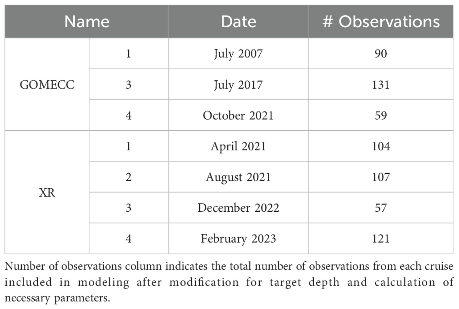
Table 1. Summary of datasets included in this research study.

From April 2021 to February 2023, five cruises were conducted in the nwGOM shelf and upper slope to collect both surface and water column data across different seasons as a part of the project “Ocean Acidification at a Crossroad” (XR) (Figure 1). Among the stations sampled were those along the Galveston transect, which is a transect along the 95° W longitude first taken during GOMECC-1 cruise. This transect was sampled on GOMECCs 3 and 4 and again by the XR project in April and August of 2021, December of 2022, and February of 2023 (Table 1; Figure 1). The combined dataset before circulations QC and preparation included 960 data points from 36 stations, out of which 94 of these data points from the GOMECC-4 cruise were to be used for testing the models while the remaining 866 data points were to be split (90:10) and used for model training and calibration.

Figure 1

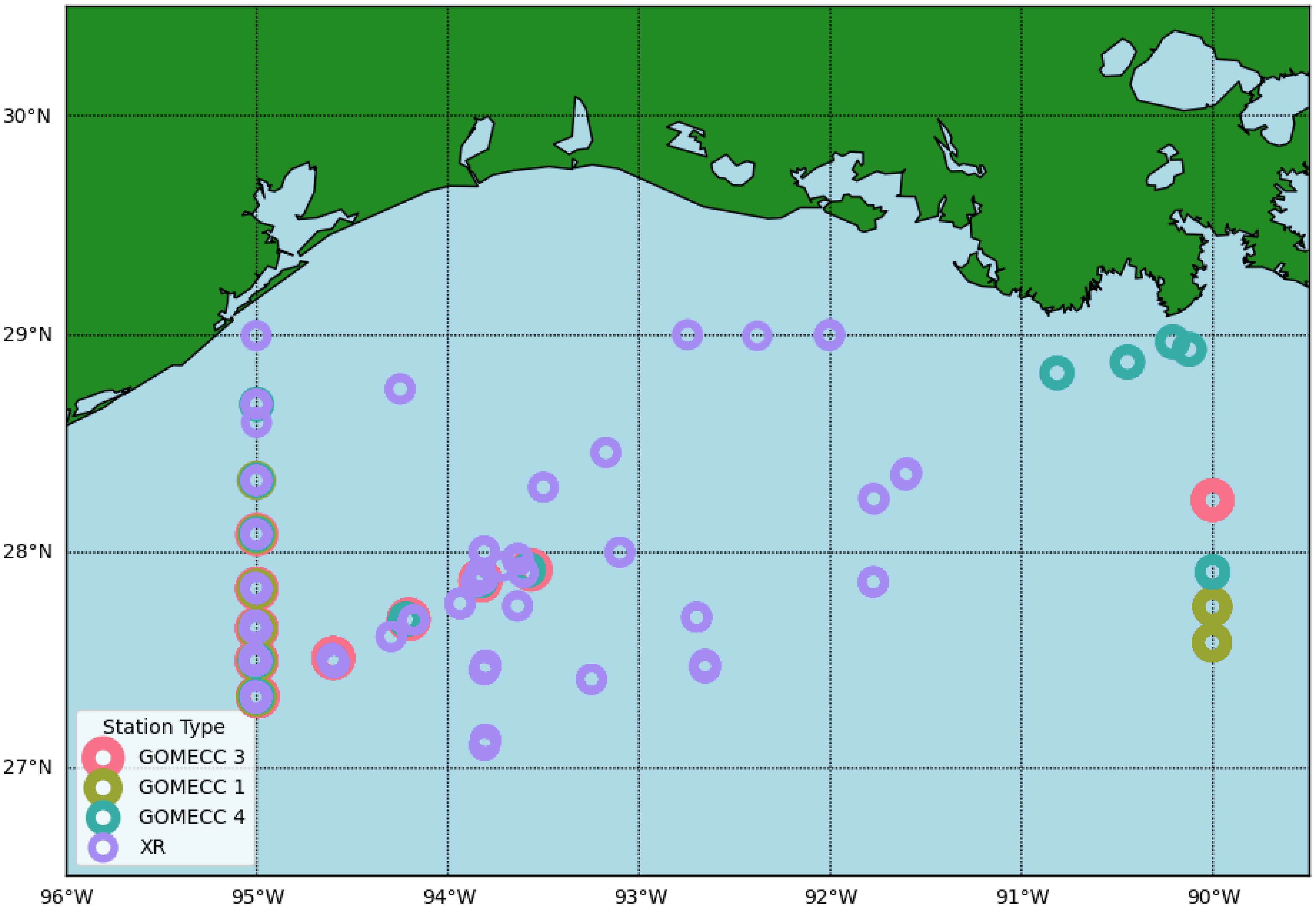
Figure 1. A map of the study area and stations where data was collected.

Sampling and analytical methods

Seawater sampling for the XR cruises was done following the best practices for carbonate chemistry analysis (Dickson et al., 2007). Briefly, samples were taken from the Niskin bottles into 250-ml ground-neck borosilicate glass bottles. Preservation of samples for carbonate chemistry analyses was done by adding 100 μl of saturated HgCl₂ solution. Glass stoppers with the aid of Apiezon^® L grease and rubber bands were used to seal the samples. The GOMECC samples were analyzed on board the ship, including DO, DIC, and TA; nutrient samples were analyzed at the Atlantic Oceanographic and Meteorological Laboratory (AOML) (Barbero et al., 2017, 2024; Peng and Langdon, 2007; Wanninkhof et al., 2012). All XR carbonate chemistry (DIC, pH, and TA) samples were analyzed in our lab at Texas A&M University-Corpus Christi (Hu et al., 2018), and DO was analyzed on board the ship. Nutrient samples were analyzed at the Geochemical and Environmental Research Group at Texas A&M University.

For the GOMECC samples, DO was determined using an automated oxygen titrator with amperometric end-point detection (Culberson and Huang, 1987). DIC was determined using gas calibrations and Certified Reference Material (CRM) stability checks to ensure proper performance (with precisions of ± 1.37 µmol/kg) (Johnson et al., 1985). For the XR samples, DO was determined on a selected subset of the samples using Winkler titration (Culberson, 1991; Winkler, 1888), as these water samples were used to verify the DO sensor on the onboard the CTD (DiMarco et al., 2012). DIC was determined using infrared methodology on a DIC analyzer (Apollo SciTech Inc.) with CRM to ensure optimal instrument performance (with precisions of ±0.1%) (Chen et al., 2015). For all cruises, TA was analyzed using open-cell Gran titration (Gran, 1952), and pH was analyzed using a spectrophotometric method with purified m-cresol purple (Liu et al., 2011). Due to the COVID-19-caused interruption to CRM supply in early 2021, XR1 samples were analyzed using CRM Batch #181 and a homemade secondary reference (based on CRM Batch #181) taken from filtered (0.2 µm) and HgCl₂-dosed Aransas Ship Channel water. XR2 samples used CRM Batch #194, 197, and 198; XR3 samples used CRM Batch #202 and 204; and XR4 samples used Batch #204 only, while XR5 samples used Batch #204 and 205.

Calculations, QC, and data preparation

Speciation calculations for the GOMECC-1 data used TA, DIC, and nutrients as input variables as direct pH measurement using the spectrophotometric method was not available. Estimated uncertainties using the average surface water conditions for pH and Ω_Arag were ±0.01 and ±0.17, respectively (Orr et al., 2018); then DIC and pH were used for speciation calculations in all other GOMECC datasets as well as the XR ones without nutrient data, resulting in an uncertainty in Ω_Arag of ±0.18. Though some calculations were done without nutrients, uncertainty contributed to the combined standard uncertainty are negligible even in high-nutrient regions, except in high-nutrient waters with TA as a member of the input pair (Orr et al., 2018). Carbonate speciation calculation was done using the MatLab version program CO2SYS (Sharp et al., 2023; van Heuven et al., 2011). Carbonate dissociation constants from Mehrbach et al. (1973) refit by Dickson and Millero (1987), the dissociation constant of bisulfate reported in Dickson et al. (1990), the total boron concentration provided in Uppström (1974), and the aragonite solubility constant from Mucci (1983) were used in these calculations. As nutrient data were not available for the XR cruises due to technical issues encountered during the pandemic, we were not able to do a strict internal consistency analysis because using TA as one of the input variables would require nutrient information. However, the offset between calculated (using DIC/pH without nutrients, except for GOMECC-1) and measured TA values, was compared across all cruises to ensure that data quality was consistent among these trips (Figure 2) (Patsavas et al., 2015).

Figure 2

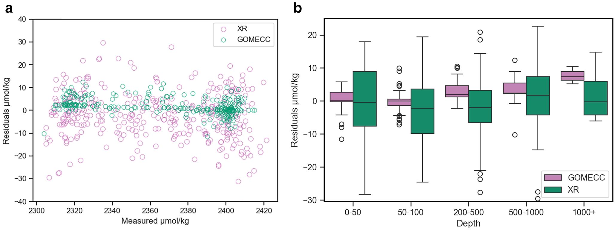
Figure 2. Visuals for quality control comparisons of analysis between XR and GOMECC datasets. Boxplot (a) showing distribution of ΔTA by calculation inputs separated by depth. Scatterplot (b) visualizing the spread of ΔTA by calculation inputs by measured TA values.

When modeling carbonate chemistry, it is crucial to focus on a geographic area where local processes and water masses exert similar control. This ensures that the relationships between parameters remain consistent throughout the area and are accurately captured in the models. Hence, data used for our model development were limited spatially within the range of 27.1–29.0˚N and 89–95.1˚W. Removal of the upper water column of various depths is regularly done in some capacity in carbonate modeling studies in an attempt to remove large, short-term, unconstrained variabilities, such as surface water gas exchange, physical, biological, and seasonal changes (Juranek et al., 2009; Kim et al., 2010; Lima et al., 2023; McGarry et al., 2021). Depth ranges of the mixed layer to be removed vary by location and season. Some models do not require exclusion of air-surface water interactions due to predictor variables being unaffected by this exchange, and others have used removal of additional surface water as a means of removing the effect of seasonality (Juranek et al., 2009; Kim et al., 2010; Lima et al., 2023; McGarry et al., 2021; Montes et al., 2016). Since the models produced in this study could contain DO, removing air-sea interaction was necessary. However, the removal of the mixed layer to eliminate seasonality as done by Kim et al. (2010) would equate to a removal of more than 100 m to account for the seasonal changes in mixed layer depth, as winter mixed layer depth in nwGOM can be more than 100 m (Muller-Karger et al., 2015). To retain as much data as possible while removing seasonality, removal of the upper 30 m of data was arbitrarily chosen. Note this removal should more than cover the depth of the mixed layer in summer but is shallower than those depths in winter and spring. The predictor parameters (salinity, temperature, pressure, and DO) were normalized to avoid collinearity, which causes computational problems that make parameter estimates unstable (Quinn and Keough, 2002). This was done through computing Z-scores using Equation 3, where X_i is the predictor variable data point, X_m is the mean of the calibration set, and X_SD is the standard deviation of the calibration set. This can be described as centering by subtracting the mean and dividing by the standard deviation, resulting in predictor variables having a mean of 0 and a standard deviation of 1.

$\begin{array}{ll}{X}_n= \frac{X_i-X_m}{X_{SD}}& (3)\end{array}$

This approach uses normalized predictor variables to estimate nonnormalized target variables, so the relative importance of multiple parameters can be compared within one model through the magnitude of the coefficients. The normalized predictor variables were tested for collinearity by calculating the variance inflation factor (VIF) for each predictor. Combinations of terms resulting in a VIF greater than 10, indicating excessive collinearity, were not used in any model (Kutner et al., 2005). Outliers were identified using studentized residuals, which are more effective for detecting outlying Y observations than standardized residuals. Studentized residuals larger than 3 (which are classified as outliers) were further examined. Each data point was individually evaluated, considering corresponding measurements from the same sample for consistency. Data flagged as questionable across multiple parameters were carefully considered, and if multiple indicators suggested potential error, the observation was excluded from the dataset. Any data points with studentized residuals >5 were removed due to the likelihood of being erroneous or anomalous.

Model creation

The modeling exercise was conducted in Python using the Scikit-learn packages (Pederegosa et al., 2011). Using a combination of the measured data (salinity or S; temperature or T; DO; and pressure, or P), these techniques produced RF and MLR models for pH and Ω_Arag. The predictor variables were selected by dredge for MLR models or variable importance for RF models (see below for details). The process was repeated until either R² values were <0.90 or only one predictor variable remained. Final predictor variable selections were used to create final models that were evaluated.

MLR - Empirical models were developed for each target variable (i.e., pH and Ω_Arag) using least squares multiple linear regression on each combination of hydrographic variables, following the methods of Juranek et al. (2009) and Alin et al. (2012). All parameters (DO, S, T, P) in the training data were given as predictors to a full MLR model. Dredge methodology was used to evaluate every possible combination of the four parameters. From among the combinations, all models were ranked based on minimizing the Akaike information criterion (AIC), a metric for model selection that incorporates both the goodness of fit and a penalty for complexity (Burnham and Anderson, 2004). The best performing models with R² > 0.90 and correlation coefficients with correct signs (±) were selected for further evaluation.

RF - An initial RF model was created including all four variables. Hyperparameter tuning is the process of optimizing a model’s configuration settings to improve performance by specifying tuned values for the number of trees, max tree depth, and minimum samples split. Hyperparameters for tuning were decided using scickit-learn GridSearchCV (Supplementary Table S2). Selected hyperparameters were applied using an RF regressor function (Probst et al., 2019). After this step, the variable importance was analyzed, and a stepwise procedure was followed to create a new model without the variable of least importance. The new model was then tuned and evaluated, if the model's R2 > 0.90 it would be considered in the final model valuation. In addition, the process starting by analyzing feature importance to create a simpler model was continued until the resulting model did not meet previously stated criteria.

Model evaluation

The models were used to predict their target variable while using predictor variable data from the completely “unseen data,” or data uninvolved in the training process, in this instance, the GOMECC-4 data. By using data from a cruise, which also took place within the time period that the modeled data were collected, separate from the training data, this ensures that the model performance results will accurately represent the models’ efficacy on new data. To ensure that the test dataset is representative of the training dataset and that the distributions of the variables are not problematically different, a two-step evaluation process was conducted. First, the distribution of each variable in both the training and test datasets was visually examined using graphical representations, such as histograms, density plots, or boxplots, to identify any noticeable differences. Second, the Kolmogorov–Smirnov (KS) test, a non-parametric statistical test, was applied to each variable to evaluate whether two samples are drawn from the same underlying distribution by comparing their cumulative distribution functions (Massey, 1951). These analyses collectively concluded that the training and test datasets are statistically comparable, minimizing the risk of bias in model evaluation due to distributional differences.

After confirmation of the representative quality of the test data, model evaluations were based on the performance across multiple metrics, including mean absolute error (MAE), mean square error (MSE), mean absolute percent error (MAPE), correlation coefficient R², and spatial bias (Vujovic, 2021). MAE and MSE represent the absolute-difference and the squared-difference metrics, respectively. MLR model variable coefficients were used for interpretation of relative variable effect. The RF model variable importance best describes model fit, not direct variable relationships, and therefore was not interpreted this way, that is, variable effect. Additional analysis of the residual data to identify normality and potential signals was done using QQ-plots and Shapiro–Wilks tests (Chen et al., 2019) (Supplementary Figures S1-S8).

Results

The models chosen to predict both Ω_Arag and pH included different combinations of the following parameters: salinity, temperature, pressure, and DO (Table 2). All linear combinations of hydrographic parameters in the models presented here resulted in VIFs less than 10, suggesting that there is no statistical evidence of coupling between any of the predictor variables. The MLR and RF models for Ω_Arag had adjusted R² values between 0.94 and 0.99 and MAE values between 0.06 and 0.14. The MLR and RF models for pH had adjusted R² values between 0.93 and 0.96 and MAE values between 0.01 and 0.02. As shown in Figures 3 and 4, the residuals for all model versions displayed some visually identifiable tendency for greater error in shallower depths. This, in combination with poorer performance of models including all depths, supports the choice made to mitigate uncertainty caused by air-sea interaction by the exclusion of the mixed layer in some capacity (Supplementary Table S2). MAPE statistics indicate the models for pH displayed less deviation between predicted and actual values and may perform better when used with new data (Table 2). These model evaluative criteria indicate that both models produced reliable results across the range of observed values in the calibration dataset (Figures 3, 4).

Table 2

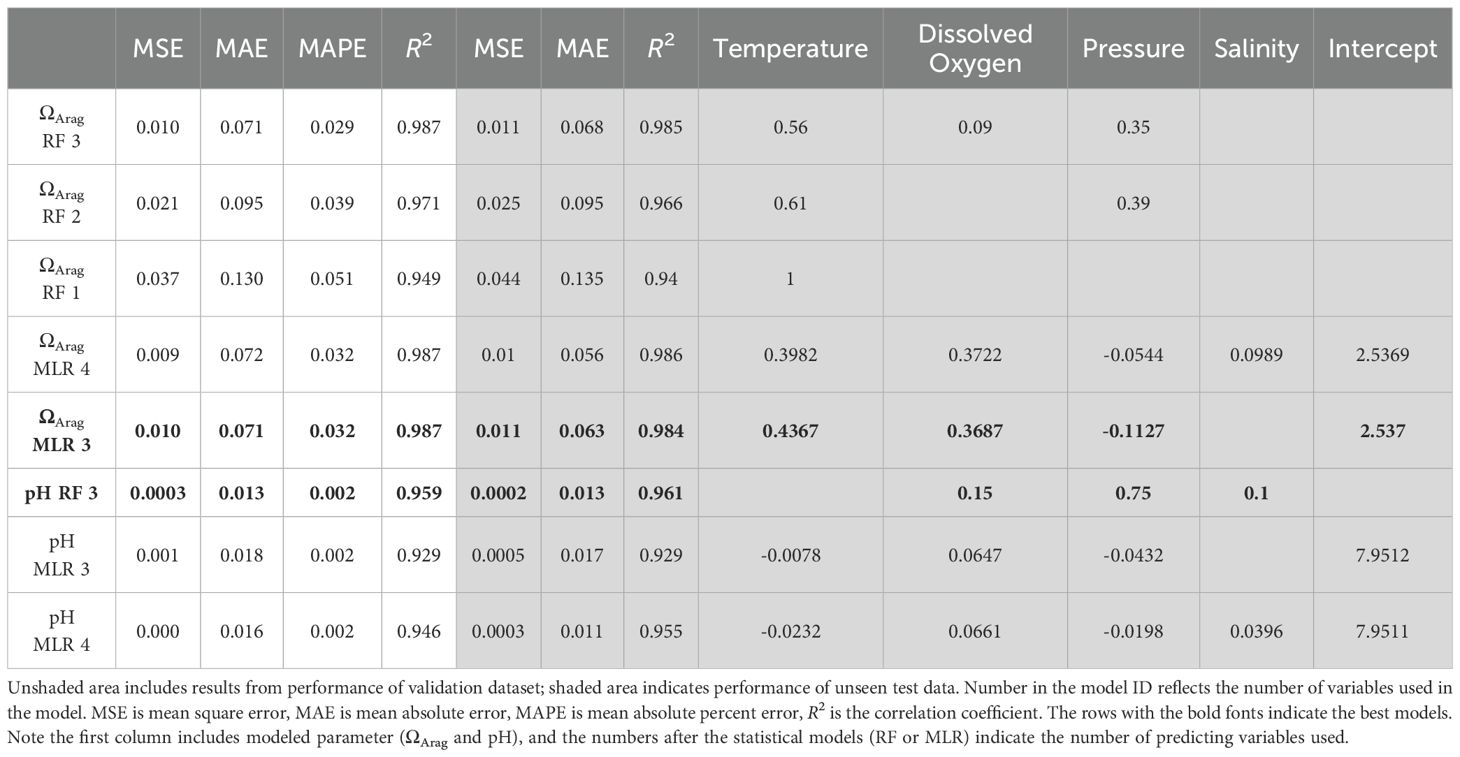
Table 2. Summary of all models for the prediction of pH including their performance metrics and variable importance for RF models and coefficients for MLR models.

Figure 3

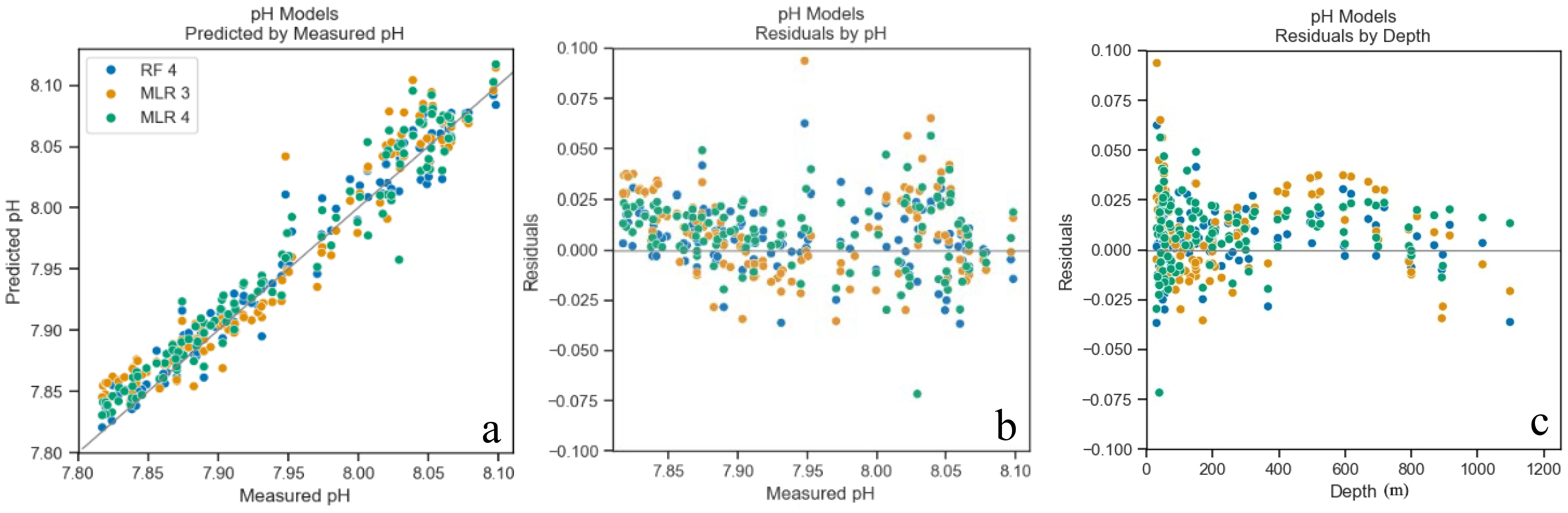
Figure 3. pH models predicted values plotted by measured values from models’ application to test dataset (GOMECC4) (a), residuals plotted by measured Ω_Arag (b), and depth (c). Points color coded for each model (Table 2).

Figure 4

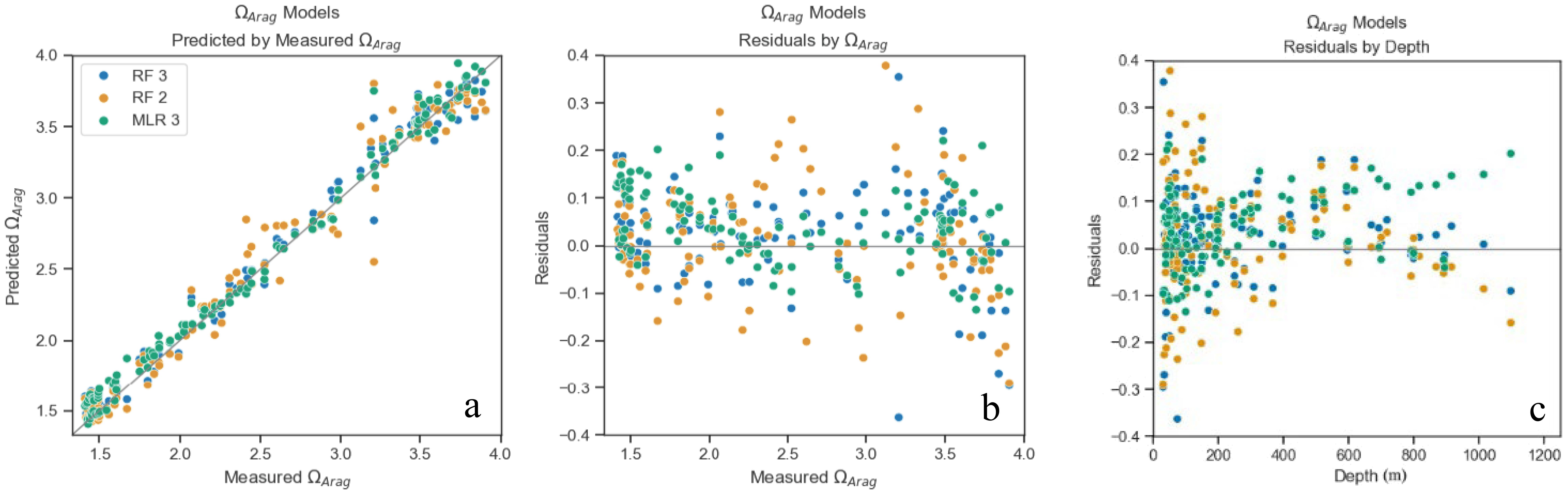
Figure 4. Ω_Arag models predicted values plotted by measured values from models’ application to test dataset (GOMECC4) (a), residuals plotted by measured Ω_Arag (b) and depth (c). Points color coded for each model (Table 2).

$\begin{array}{ll}{E}_{est}=\sqrt{E_{Response}^2+E_{Input}^2+E_{MLR}^2}& (4)\end{array}$

$\begin{array}{ll}{E}_{est}=\sqrt{{\sum }_{i=1}^n{(U_i{B}_i)}^2}& (5)\end{array}$

Uncertainty propagations were calculated using Equation 4 (Carter et al., 2018; Li et al., 2022). E_MLR refers to the model RMSE. E_Response represents measurement uncertainties; for pH, this is the spectrophotometric measurement uncertainty, which was set conservatively to be a constant 0.005 (Carter et al., 2024). For Ω_Arag this is the uncertainty from input pairs propagated through calculations of Ω_Arag which was set as 0.085 (Orr et al., 2018). E_input is the uncertainty of the input parameters propagated in the regression, which can be calculated using Equation 5, where U_i is the i-th input uncertainties of the predictor properties. We set the U_i values at 0.005, 0.005°C, and 2.2 µmol kg⁻¹ for S, T, and DO, respectively (Carter et al., 2018). Total uncertainty calculated is 0.12 for Ω_Arag and 0.0173 for pH. Other information that can be inferred from these calculations is the relative sources of uncertainty by the comparison of E_Response, E_Input, and E_MLR. In both cases the E_MLR value was the largest contributor of uncertainty, followed by E_Response.

In addition to the total uncertainty calculations, a better understanding of the source of the uncertainty described by the E_MLR can be achieved by examining the calculations of error used to describe model performance, such as MAPE and MAE. Ω_Arag models produced MAPE scores of 2.9%–5.1% and MAE of 0.05–0.13 in comparison to estimates of error propagation for calculation of Ω_Arag being ±0.16 depending on input pairs (Orr et al., 2018). Most of the uncertainty from calculation comes from the pair-constants curve, meaning methodological uncertainties for the input pairs result in little effect on the overall propagated uncertainties. Therefore, the relative uncertainty due to error of model Ω_Arag values has similar reliability to calculations of Ω_Arag from measured DIC, TA, or pH values. This was not true for pH models, as MAPE scores ranged from 0.16% to 0.22%, with an MAE of 0.011–0.018 in comparison to a relative uncertainty of measurement methods of 0.008–0.0012, meaning that there is a higher confidence of measured values as opposed to predicted (Takeshita et al., 2021).

The best model for Ω_Arag was the MLR model, which included all variables with an R² = 0.99. (Ω_Arag MLR 4; Table 2). MLR equation coefficients indicate that for the Ω_Arag model, variable importance, or contribution to explainability, is as follows, from most to least important: temperature, DO, pressure, and salinity, with temperature and DO being >77% larger than pressure and salinity. The second-best performing model with R² = 0.98 is the MLR model with three variables, which, in order of importance, are temperature, DO, and pressure (Ω_Arag MLR 3; Table 2). The RF models did not outperform MLR models but came close behind, with the best RF model (Ω_Arag RF 3; Table 2) having an R² = 0.99 while using the same three variables as the second-best MLR model. For the RF models, poorer performance on test data than validation data would indicate overfitting and that the model has poor ability to generalize. However, minimal difference (ΔR² < 0.01) was observed in performance on testing versus validation data. This indicates that the model is not overfitted, generalized well, and can be expected to perform similarly (as it did on the test data) on new data (Domingos, 2012).

For pH, the best-performing model was the RF model that included three variables with an R² = 0.96. (pH RF 3; Table 2). The second-best performing model with R² = 0.975 was the MLR model with all variables, which, in order of importance, are DO, temperature, pressure, and salinity (pH MLR 4). The RF models outperformed the MLR models for pH prediction, but again by a narrow gap. Differences were observed in performance on validation and test datasets of R² > 0.6, indicating which models may be slightly overfitted. The RF model containing all four variables performed poorly, possibly due to overfitting or collinearity and thus is not included.

All residuals indicated nonnormality as seen in QQ-plots, histograms, and through Shapiro-Wilks p-values < 0.05 (Supplementary Figures S1–S8). To further investigate the non-normality of residuals and determine if it could be an indicator of other problems, the Durbin-Watson and Breusch-Pagan tests were used to test the assumptions for independent and homoscedastic residuals. A Durbin-Watson test for independence resulting in a value close to 2 suggests that the residuals an autocorrelated. Breusch–Pagan test for homoscedasticity, where a p > 0.05 suggests homoscedasticity. Therefore, despite the nonnormality of the residuals, it is unlikely to be problematic due to their independence, homoscedasticity, the size of the dataset, and the robust nature of the models (Breiman, 2001).

Discussion

Data selection considerations

The nwGOM area (latitudes 27.1–29.0˚N and longitudes 89–95.1˚W) was selected to isolate a relatively small geographic area where controlling factors on the carbonate system are expected to remain similar in the examined window of time and included the same stations surveyed repeatedly along the same transect (i.e., the 90° line). This study area lies almost entirely on the Texas shelf and far enough to the west so that the effects of the freshwater discharge transported westward are less pronounced than on the bulk of the Louisiana Shelf (Androulidakis et al., 2015; Morey et al., 2003). Under heavy influence from the large river’s watershed, salinity would be a key variable for models, although it is not detected as such in our models. Therefore, salinity was only included as a predictor variable in one of the Ω_Arag models and only half of the pH models.

Removal of the surface layer of the water column was done strategically to remove large, short-term temporally unconstrained variabilities, such as surface water gas exchange, physical, biological, and seasonal changes (Juranek et al., 2009; Kim et al., 2010; McGarry et al., 2021). In the nwGOM, removal of shallow water can potentially mitigate the minimal effects of freshwater outflow as the low-salinity river discharge is buoyant. Removal of surface water can be less important when air-surface water interactions do not affect predictor variables. Even still, removal can serve as a means of removing the effect of seasonality, though depth ranges of the mixed layer to be removed vary by location and season (Juranek et al., 2009; Kim et al., 2010; McGarry et al., 2021; Montes et al., 2016). Since most of the models produced in this study contain DO, removing air-sea interaction was necessary. Based on the final models chosen for Ω_Arag and pH, the relationships showed that the exclusion of the upper 30 m of the water column did improve the performance of all Ω_Arag models. When models are compared with the model containing the same spatial data but all depths, models with the upper 30 m removed, except for pH MLR models, had either greater R², lower MSE or MAPE, or a combination of the three (Supplementary Table S2). The improvements in all models indicate that the removal of surface water increases the performance of the models, though it should be noted that there may be bias across seasons due to unaccounted-for surface water and mixed-layer inclusion in the datasets used for training. Seasonal bias could also occur due to a greater quantity of summer observations in the training dataset. Further data beyond the 2007–2023 time series, as well as the inclusion of more seasonal data, are needed to properly assess the potential existence of these biases.

Aragonite models

There are many known relationships between Ω_Arag and physical and chemical parameters, which is why the variables salinity, temperature, pressure, and DO were chosen in developing Ω_Arag models. However, the degree to which each of these variables is intertwined with Ω_Arag is not so easy to identify but can be inferred by their selection and importance in the models with the highest performance.

Temperature was the most prominent predictor for Ω_Arag in all models (Table 2). The strength of the relationship can be explained by Ω_Arag as a function of K_sp and [CO₃²⁻], and K_sp as a function of temperature, salinity, and pressure. Temperature as a dominant predictor variable aligns well with models built for Ω_Arag prediction in other areas, which also found temperature to be a primary predictor for Ω_Arag (Alin et al., 2012; Juranek et al., 2009; Kim et al., 2010; McGarry et al., 2021). Pressure was included in all MLR models and two out of three RF models (Table 2). The pressure term in the models can be in part explained by Ω_Arag as a function of K_sp and [CO₃²⁻], and K_sp is also a function of pressure, that is, increasing solubility with depth. DO was included in both MLR models and one RF model (Table 2). The inclusion of DO is likely due to the close coupling of DO and DIC in subsurface waters, which includes CO₂ uptake (photosynthesis) and release (respiration) and lacks exchange with the atmosphere in the subsurface (>30 m). Although salinity was also tested, it was only included in one MLR model based on selection criteria and was the least important predictor variable by coefficient (Table 2). The lack of salinity could be in part because salinity in the modeled dataset has small variability from 33.2 to 36.7 without outliers and an interquartile range (IQR) of from 35.2 to 36.4. This means salinity has a relatively small contribution to variability, either due to the hydrography of the area or possibly in part to the limitation of the dataset’s spatial and depth coverage. By focusing on the nwGOM and removing the upper 30 m it is possible that freshwater outflow transported from the Mississippi-Atchafalaya watershed westward over the Louisiana-Texas shelf in the surface water has been partially or wholly avoided (Morey et al., 2003).

pH models

Although anthropogenic CO₂ is the dominant driver for long‐term, that is, multidecadal, change in pH in the upper ocean water column, the variations observed in coastal waters on decadal time scales are largely attributed to driving forces including production shift due to changes in nutrient input (Wang et al., 2013) and ocean circulation changes (e.g., upwelling) (Feely et al., 2008) and terrestrial influences (Cai, 2003; Duarte et al., 2013; Gomez et al., 2021). The fact that DO was included as an important predictor variable suggests that biological activities are a major driving force for the carbonate system. Similarly, DO was also found to be the strongest predictor of pH in the Northeast US (McGarry et al., 2021). Pressure was also important in all the models, as carbonate system equilibria are affected by pressure (Table 2). There is a visually notable trend of overprediction of pH from 400 to 800 m; this is an area with lower pH and Ω than the rest of the water column. We attribute this bias to the non-linearity of the carbonate system. This type of bias has also been seen in other similar models in different geographic locations as well (Juranek et al., 2011, 2009).

Comparison with previous models

One of the primary motivations behind the use of the MLR modeling with standardized variables is the ability to use empirical relationships among predictor variables to accurately describe the controlling processes in the study area, whereas RF modeling can only provide relative feature importance, which is not a quantification of the correlation between variables but of the relative impact on the performance of the model, or reduced impurity, that can be attributed to that predictor variable (Breiman, 2001). Due to standardization, the strength of the predictor variable correlation with the target variable can be inferred by the absolute value of the coefficients of predictor variables included in the models. However, it is important to note that statistical models reflect correlations between predictor variables and target variables but do not necessarily reveal mechanistic relationships (Quinn and Keough, 2002) (Table 2).

Because of differences in hydrography, river influences, and location of the drivers of the carbonate system, statistical models for carbonate system parameters are often specific to the geographic areas where they were created for. Although many of the primary drivers of the carbonate system remain the same, the secondary variables shift, as does the degree to which they influence.

In the literature, Ω_Arag models have been created for the northwestern Atlantic (McGarry et al., 2021), northern Gulf of Alaska (Evans et al., 2013), Central Oregon Coast (Juranek et al., 2011, 2009), southern California Current system (Alin et al., 2012), Queen Charlotte Sound (Hare et al., 2025), U.S. east coast (Li et al., 2022), and the Sea of Japan (East Sea) (Kim et al., 2010). These models all have between two and three variables and an adjusted R² ≥ 0.91 compared to between one and four variables with an adjusted R² ≥ 0.94 in this study. The primary predictor variable in all previous models except two (Evans et al., 2013; Juranek et al., 2011) is temperature, as is the case in this study. Most models also include some combination of temperature with salinity, oxygen, and interaction terms; one model also used pressure (Kim et al., 2010), and one used NO₃^- (Evans et al., 2013). The models created here and those created previously for Ω_Arag agreed on the use of temperature as a primary predictor variable in combination with other predictor variables.

pH models have been created for the eastern US coast (McGarry et al., 2021; Li et al., 2022), the northeast Pacific (Juranek et al., 2011), the southern California Current System (Alin et al., 2012), Queen Charlotte Sound (Hare et al., 2025), and the global ocean (Carter et al., 2021). All those models also used temperature and DO (Alin et al., 2012; Juranek et al., 2011; McGarry et al., 2021; Li et al., 2022), with one model also using an interaction term between DO and temperature (Alin et al., 2012), one using nutrients, salinity, and multiple interaction terms (McGarry et al., 2021) and, lastly, one using AOU and salinity (Hare et al., 2025). They included between two and seven variables and resulted in adjusted R² ≥ 0.89 in comparison to our models, which have between three and four variables and adjusted R² ≥ 0.93. Our MLR models are consistent with previous models that DO was an important predictor variable for pH.

Model applicability

The GOMECC-1 survey in 2007 was among the first to collect comprehensive, high-quality, measurements of the inorganic carbonate system parameters in the GOM. However, the capacity for autonomous observation of ocean carbonate chemistry is growing rapidly. By combining real-time, high-resolution data with modeling methods, it is possible to create comprehensive data coverage while simultaneously providing data validation via comparison between different data sources. With the use of MLR in combination with a single Argo profile float containing DO and temperature sensors, Juranek et al. (2011) were able to create a 14-month comprehensive time series containing Ω_Arag and pH, which were verified by comparisons to independently measured values. Evans et al. (2013) applied models to field data from glider flight and a GLOBEC mesoscale SeaSoar survey (Cowles, 2002) to create complete datasets, allowing for identification of variability of Ω_Arag. Hare et al. (2025) also had success with this in Queen Charlotte Sound, British Columbia, where regression models were applied to regional autonomous glider data. Although autonomous measurements for biogeochemical parameters in the GOM have just begun (Osborne et al., 2024), successful combination of models and autonomous data collection should greatly improve geochemical data coverage and advance carbonate chemistry studies.

In addition to long-term changes, there is strong motivation to apply empirical models to year-round hydrographic data to reconstruct the seasonal cycle of carbonate chemistry. For example, Juranek et al. (2009) created a model using data collected in spring and successfully used it to predict the seasonal changes in Ω_Arag under the assumption that the seasonal variability of the primary independent variables (temperature and DO) would be comparable to the variations encountered spatially during the initial data collection. One method to mitigate effects of the lack of seasonal variation data on the relationships between physical and chemical data is by excluding depths influenced by local meteorological conditions from the analysis (Kim et al., 2010). Most models were calibrated using mostly summer data and none with subsurface seasonal data for the GOM. Our models contain data from all seasons with slightly more data points from summer months. Seasonal application is expected to be viable in the produced models for pH as it was explained primarily by biologically driven changes, that is, the coupling between DIC and DO. Seasonal application is also expected to be viable for Ω_Arag at depths of 30–300 m, as biological changes are primarily driven by DIC rather than TA (Anglès et al., 2019; Hu et al., 2018). It is expected that changes in DIC should be captured in these models due to their relationship with DO in the subsurface (Anderson and Sarmiento, 1994; Hales et al., 2005).

Furthermore, there is also motivation to apply statistical models to forecast the carbonate system conditions as OA progresses. Previously created MLRs have been applied to generate hindcasts (up to 40 years) on carbonate chemistry (Evans et al., 2013; Kim et al., 2010). However, the temporal applicability of a model is expected to be limited. To use the model for predictions beyond the timeframe of training data, even with relatively unchanged circulation and watershed conditions, it is necessary to make corrections for shifts caused by changes in the anthropogenic CO₂ inventory in the water column, increasing error beyond model uncertainty. This is because empirical models do not account for anthropogenic addition of CO₂, which changes the ratio of DIC/DO. Due to atmospheric CO₂ input, previous modeling studies have calculated that the statistical relationships will need to be updated every 5–10 years to account for changes in target variables (Alin et al., 2012; Juranek et al., 2011, 2009). The models can be used for estimation of data within the timeframe of the training data (2007–2023), with the requirement that seasonality or waterbody changes are captured, hindcasting up to 10 years (1997–2007), and predicting up to 10 years (2023–2033) (Juranek et al., 2011). For example, Juranek et al. (2009) created a model using data collected in spring, and they successfully used it to predict the seasonal changes in Ω_Arag. The assumption of this study was that the seasonal variability of the primary independent variables (temperature and DO) would be comparable to the variation encountered spatially during the initial data collection just a year prior. However, to extend the reconstruction further than 10 years, it would be necessary to account for the progressive addition of anthropogenic CO₂ to the water column over time. For example, Kim et al. (2010) used estimates of anthropogenic CO₂ invasion to subtract anthropogenic CO₂ and apply modeling estimates of DIC in the Sea of Japan (East Sea) to create a 40-year reconstruction. In our study, the total uncertainty values are 0.12 for Ω_Arag and 0.0173 for pH. The rate of pH decline at the surface during the 2013–2022 period is 0.0025 ± 0.0005 year¹⁻, while there is no discernable trend in Ω_Arag (Hu, unpublished data). Based on this, it would take 14 years for the accumulation of anthropogenic carbon to surpass two times the uncertainty for pH (i.e., the time of emergence, Turk et al., 2019). Due to the lack of trend in Ω_Arag, these models could be applicable for a longer period in this region. However, we recommend conservatively applying caution when using beyond the 10-year window. For all models but particularly Ω_Arag, it seems likely that other factors such as changing climatology may be the first to influence model applicability rather than anthropogenic CO₂ intrusion.

Data scarcity

Technological advancements (e.g., satellites, floats, and gliders) have made autonomous measurements for selected variables possible. Even though satellites provide large volumes of invaluable data, their scope is limited not only to the surface layer but also to measurements of temperature and ocean color, which can be used for estimations of productivity, dissolved organic matter, and sea surface CO₂ partial pressure (e.g., Chen et al., 2019). Some remedies for the lack of data beyond the surface have come in the form of novel technologies, including Argo floats and gliders (Osborne et al., 2024). The Argo array supports more than 3,000 floats across the global ocean, supplying profiles of T and S, of which about 200 are also equipped with a DO sensor. Biogeochemical-Argo (BGC-Argo) floats can take measurements from the surface to 2,000 dbar and provide high-resolution autonomous measurements for some combinations of chlorophyll, particle backscatter, DO, nitrate, pH, or irradiance (Roemmich et al., 2019). Nevertheless, this equipment is limited in coverage ability; BGC-Argos have yet to reach the comprehensive coverage of traditional Argos, and they usually do not operate on continental shelves. Gliders share the similar biogeochemical sensors used by the BGC-Argo floats with a similar mode of operation but perform sawtooth trajectories from the surface to the bottom, or to 200–1,000 m depth, and their deployments are limited largely by biofouling, battery life, and payload space, hindering their ability to carry many sensors (Saba et al., 2019; Testor et al., 2019). Additionally, all data from floats and gliders must undergo rigorous quality control and correction of potential errors in sensors, such as drift and be compared to lab-measured samples when possible (Roemmich et al., 2019).

Given the performance of the models created here, it would be reasonable to expect that in combination with datasets from data collection via these platforms, one or both of pH and Ω_Arag could be estimated. Traditional Argos, as well as most gliders, have temperature and pressure (or depth) measurements, meaning Ω_Arag could be estimated using either of the two RF models with R² values of 0.94 and 0.97. With the addition of DO, which is included in a subset of the Argos and in the BGC-Argos, the Ω_Arag model with an R² of 0.98 could be applied. Additionally, the pH model with R² of 0.94 could be used; even though pH sensors are included in many BGC-Argos, the modeled results could provide robust data quality check capability.

Recommendations

The models developed in this study serve as valuable tools for reconstructing pH and Ω_Arag data in the absence of direct chemical observations, leveraging available hydrographic information. The models can also be used for hindcasting over a 10-year period (1997–2007) and for forecasting over the next ~10 years (2023–2033) in the nwGOM, if seasonality and watermass changes are adequately captured. Through modeling, our results showed that RF models do not have any distinct advantage over the MLR models which are commonly used. It is crucial to examine potential shifts in circulation, water mass composition, and anthropogenic CO₂ accumulation to refine and update the models over time. Despite their robustness, several potential issues remain across all models, suggesting room for improvement, such as difficulties estimating target variables due to significant variation in the shallow and mixed layers, a need for additional data points, or the application of more complex models. Future work to enhance these models could involve incorporating additional data, as well as exploring the application of neural network AI models and locally interpolated regressions, such as those employed by Carter et al. (2021).

Data availability statement

The original contributions presented in the study are publicly available. This data can be found here: https://github.com/ejundt/XRModel.git and https://wq.gcoos.org/oa/data/csv/. Publicly available datasets were analyzed in this study. This data can be found here: https://glodap.info/.

Author contributions

EJ: Conceptualization, Data curation, Formal analysis, Investigation, Methodology, Software, Validation, Visualization, Writing – original draft, Writing – review & editing. XH: Conceptualization, Funding acquisition, Resources, Supervision, Writing – review & editing.

Funding

The author(s) declare financial support was received for the research and/or publication of this article. This study was funded by NOAA Ocean Acidification Program (award #NA19OAR0170354).

Acknowledgments

This publication was made possible by the National Oceanic and Atmospheric Administration, Office of Education Educational Partnership Program with Minority Serving Institutions award (NA21SEC4810004). We would like to thank Steven DiMarco, Piers Chapman, Sakib Mahmud, students and postdocs from Texas A&M University, and the captain and crew on board R/V Pelican for their assistance with sample collection and analyses. We would also like to thank the scientific party on previous GOMECC cruises for their contributions to the data used in this study.

Conflict of interest

The authors declare that the research was conducted in the absence of any commercial or financial relationships that could be construed as a potential conflict of interest.

Generative AI statement

The author(s) declare that no Generative AI was used in the creation of this manuscript.

Any alternative text (alt text) provided alongside figures in this article has been generated by Frontiers with the support of artificial intelligence and reasonable efforts have been made to ensure accuracy, including review by the authors wherever possible. If you identify any issues, please contact us.

Publisher’s note

All claims expressed in this article are solely those of the authors and do not necessarily represent those of their affiliated organizations, or those of the publisher, the editors and the reviewers. Any product that may be evaluated in this article, or claim that may be made by its manufacturer, is not guaranteed or endorsed by the publisher.

Author disclaimer

Its contents are solely the responsibility of the award recipient and do not necessarily represent the official views of the U.S. Department of Commerce, National Oceanic and Atmospheric Administration.

Supplementary material

The Supplementary Material for this article can be found online at: https://www.frontiersin.org/articles/10.3389/fmars.2025.1621280/full#supplementary-material

References

Alin S. R., Feely R. A., Dickson A. G., Martín Hernández-Ayón J., Juranek L. W., Ohman M. D., et al. (2012). Robust empirical relationships for estimating the carbonate system in the southern California Current System and application to CalCOFI hydrographic cruise data, (2005–2011). J. Geophys Res. Oceans 117, 5033. doi: 10.1029/2011JC007511

Crossref Full Text | Google Scholar

Anderson L. A. and Sarmiento J. L. (1994). Redfield ratios of remineralization determined by nutrient data analysis. Global Biogeochem Cycles 8, 65–80. doi: 10.1029/93GB03318

Crossref Full Text | Google Scholar

Androulidakis Y. S., Kourafalou V. H., and Schiller R. V. (2015). Process studies on the evolution of the Mississippi River plume: Impact of topography, wind and discharge conditions. Cont Shelf Res. 107, 33–49. doi: 10.1016/j.csr.2015.07.014

Crossref Full Text | Google Scholar

Anglès S., Jordi A., Henrichs D. W., and Campbell L. (2019). Influence of coastal upwelling and river discharge on the phytoplankton community composition in the northwestern Gulf of Mexico. Prog. Oceanogr 173, 26–36. doi: 10.1016/j.pocean.2019.02.001

Crossref Full Text | Google Scholar

Barbero L., Pierrot D., Wanninkhof R., Baringer M., Hooper J., Zhang J. Z., et al. (2017). Cruise Report: Third Gulf of Mexico Ecosystems and Carbon Cycle (GOMECC-3) Cruise. Miami, FL 33149: NOAA Atlantic Oceanographic and Meteorological Laboratory. doi: 10.25923/y6m9-fy08

Crossref Full Text | Google Scholar

Barbero L., Stefanick A., Hooper J., Wanninkhof R., Baringer M., Smith I., et al. (2024). Cruise Report: Fourth Gulf of Mexico Ecosystems and Carbon Cycle (GOMECC-4) Cruise. Atlantic Oceanographic and Meteorological Laboratory, Miami, FL 33149. doi: 10.25923/rwx5-s713

Crossref Full Text | Google Scholar

Bednaršek N., Tarling G. A., Bakker D. C. E., Fielding S., Jones E. M., Venables H. J., et al. (2012). Extensive dissolution of live pteropods in the Southern Ocean. Nat. Geosci 5, 881–885. doi: 10.1038/NGEO1635

Crossref Full Text | Google Scholar

Bostock H. C., Mikaloff Fletcher S. E., and Williams M. J. M. (2013). Estimating carbonate parameters from hydrographic data for the intermediate and deep waters of the Southern Hemisphere oceans. Biogeosciences 10 (10), 6199–6213. doi: 10.5194/BG-10-6199-2013

Crossref Full Text | Google Scholar

Breiman L. (2001). Random forests. Mach. Learn 45, 5–32. doi: 10.1023/A:1010933404324/METRICS

Crossref Full Text | Google Scholar

Burnham K. P. and Anderson D. R. (2004). Multimodel inference: understanding AIC and BIC in model selection. Sociological Methods & Research 33, 261–304. doi: 10.1177/0049124104268644

Crossref Full Text | Google Scholar

Cai W. J. (2003). Riverine inorganic carbon flux and rate of biological uptake in the Mississippi River plume. Geophys Res. Lett. 30, 1032. doi: 10.1029/2002GL016312

Crossref Full Text | Google Scholar

Cai W. J., Hu X., Huang W. J., Murrell M. C., Lehrter J. C., Lohrenz S. E., et al. (2011). Acidification of subsurface coastal waters enhanced by eutrophication. Nat. Geosci. 11, 766–770. doi: 10.1038/ngeo1297

Crossref Full Text | Google Scholar

Cai W. J., Xu Y. Y., Feely R. A., Wanninkhof R., Jönsson B., Alin S. R., et al. (2020). Controls on surface water carbonate chemistry along North American ocean margins. Nat. Commun. 11, 1–13. doi: 10.1038/s41467-020-16530-z

PubMed Abstract | Crossref Full Text | Google Scholar

Carter B. R., Bittig H. C., Fassbender A. J., Sharp J. D., Takeshita Y., Xu Y.-Y., et al. (2021). New and updated global empirical seawater property estimation routines. Limnology and Oceanography: Methods. 19, 785–809. doi: 10.1002/lom3.10461

Crossref Full Text | Google Scholar

Carter B. R., Feely R. A., Williams N. L., Dickson A. G., Fong M. B., and Takeshita Y. (2018). Updated methods for global locally interpolated estimation of alkalinity, pH, and nitrate. Limnol Oceanogr Methods 16, 119–131. doi: 10.1002/LOM3.10232;JOURNAL:JOURNAL:15415856;WGROUP:STRING:PUBLICATION

Crossref Full Text | Google Scholar

Carter B. R., Sharp J. D., Dickson A. G., Álvarez M., Fong M. B., García-Ibáñez M. I., et al. (2024). Uncertainty sources for measurable ocean carbonate chemistry variables. Limnol Oceanogr 69, 1–21. doi: 10.1002/LNO.12477

Crossref Full Text | Google Scholar

Chen B., Cai W. J., and Chen L. (2015). The marine carbonate system of the Arctic Ocean: Assessment of internal consistency and sampling considerations, summer 2010. Mar. Chem. 176, 174–188. doi: 10.1016/J.MARCHEM.2015.09.007

Crossref Full Text | Google Scholar

Chen S., Hu C., Barnes B. B., Wanninkhof R., Cai W.-J., Barbero L., et al. (2019). A machine learning approach to estimate surface ocean pCO 2 from satellite measurements. Remote Sens Environ. 228, 203–226. doi: 10.1016/j.rse.2019.04.019

Crossref Full Text | Google Scholar

Cowles T. (2002). GLOBEC Northeast Pacific California Current Cruise Report, R/V Thomas G. Thompson (T0205) Alternative Cruise ID: Mesoscale Survey TN147 Chief Scientist: Cruise Objectives. College of Oceanic and Atmospheric Sciences Oregon State University Corvallis, OR.

Google Scholar

Culberson C. H. (1991). WHO Operations and Methods: Dissolved Oxygen. Newark. College of Marine Studies. University of Delaware. Newark, U.S.A.

Google Scholar

Culberson C. H. and Huang S. (1987). An automated amperometric oxygen titration. Deep Sea Res. 34, 875–880. doi: 10.1016/0198-0149(87)90042-2

Crossref Full Text | Google Scholar

Cutler D. R., Edwards T. C., Beard K. H., Cutler A., Hess K. T., Gibson J., et al. (2007). Random forests for classification in ecology. Ecology 88, 2783–2792. doi: 10.1890/07-0539.1

PubMed Abstract | Crossref Full Text | Google Scholar

Dickson A. G. and Millero F. J. (1987). A comparison of the equilibrium constants for the dissociation of carbonic acid in seawater media. Deep Sea Research Part A, Oceanographic Research Papers 34 (10), 1733–1743. doi: 10.1016/0198-0149(87)90021-5

Crossref Full Text | Google Scholar

Dickson A. G., Wesolowski D. J., Palmer D. A., and Mesmer R. E. (1990). Dissociation constant of bisulfate ion in aqueous sodium chloride solutions to 250°C. J. Physical Chem. 94 (20), 7978–7985. doi: 0.1021/J100383A042/ASSET/J100383A042.FP.PNG_V03

Google Scholar

Dickson A. G., Sabine C. L., and Christian J. R. (2007). “Guide to best practices for ocean CO2 measurements,” in PICES Special Publication, Guide to Best Practices for Ocean CO2 measurements (North Pacific Marine Science Organization Sidney, British Columbia, Canada: PICES Special Publication).

Google Scholar

DiMarco S. F., Strauss J., May N., Mullins-Perry R. L., Grossman E. L., and Shormann D. (2012). Texas coastal hypoxia linked to Brazos river discharge as revealed by oxygen isotopes. Aquat Geochem 18, 159–181. doi: 10.1007/S10498-011-9156-X/METRICS

Crossref Full Text | Google Scholar

Domingos P. (2012). A few useful things to know about machine learning. Commun. ACM. 55 (10), 78–87. doi: 10.1145/2347736.2347755

Crossref Full Text | Google Scholar

Duarte C. M., Hendriks I. E., Moore T. S., Olsen Y. S., Steckbauer A., Ramajo L., et al. (2013). Is ocean acidification an open-ocean syndrome? Understanding anthropogenic impacts on seawater pH. Estuaries Coasts 36, 221–236. doi: 10.1007/S12237-013-9594-3/TABLES/1

Crossref Full Text | Google Scholar

Erez J., Reynaud S., Silverman J., Schneider K., and Allemand D. (2011). “Coral calcification under ocean acidification and global change,” in Coral Reefs: An Ecosystem in Transition (Springer Dordrecht, Netherlands: Springer Netherlands), 151–176. doi: 10.1007/978-94-007-0114-4_10

Crossref Full Text | Google Scholar

Evans W., Mathis J. T., Winsor P., Statscewich H., and Whitledge T. E. (2013). A regression modeling approach for studying carbonate system variability in the northern Gulf of Alaska. J. Geophys Res. Oceans 118, 476–489. doi: 10.1029/2012JC008246

Crossref Full Text | Google Scholar

Eyre B. D., Andersson A. J., and Cyronak T. (2014). Benthic coral reef calcium carbonate dissolution in an acidifying ocean. Nat. Climate Change 11, 969–976. doi: 10.1038/nclimate2380

Crossref Full Text | Google Scholar

Feely R. A., Sabine C. L., Hernandez-Ayon J. M., Ianson D., and Hales B. (2008). Evidence for upwelling of corrosive “acidified” water onto the continental shelf. Science (1979) 320, 1490–1492. doi: 10.1126/science.1155676

PubMed Abstract | Crossref Full Text | Google Scholar

Gomez F. A., Wanninkhof R., Barbero L., and Lee S. K. (2021). Increasing river alkalinity slows ocean acidification in the northern Gulf of Mexico. Geophys Res. Lett. 48, e2021GL096521. doi: 10.1029/2021GL096521

Crossref Full Text | Google Scholar

Gran G. (1952). Determination of the equivalence point in potentiometric titrations. Part II Analyst 77, 661–671. doi: 10.1039/an9527700661

Crossref Full Text | Google Scholar

Hales B., Takahashi T., and Bandstra L. (2005). Atmospheric CO2 uptake by a coastal upwelling system. Global Biogeochem Cycles 19, 1–11. doi: 10.1029/2004GB002295

Crossref Full Text | Google Scholar

Hare A. A., Evans W., Dosser H. V., Jackson J. M., Alin S. R., Hannah C., et al. (2025). Regression-based characterization of the marine carbonate system across shelf and nearshore waters of Queen Charlotte Sound. Mar. Chem. 270, 104511. doi: 10.1016/J.MARCHEM.2025.104511

Crossref Full Text | Google Scholar

Hoegh-Guldberg O., Mumby P. J., Hooten A. J., Steneck R. S., Greenfield P., Gomez E., et al. (2007). Coral reefs under rapid climate change and ocean acidification. Science 318, 1737–1742. doi: 10.1126/SCIENCE.1152509/SUPPL_FILE/HOEGH-GULDBERG.SOM.PDF

Crossref Full Text | Google Scholar

Hu X., Li Q., Huang W. J., Chen B., Cai W. J., Rabalais N. N., et al. (2017). Effects of eutrophication and benthic respiration on water column carbonate chemistry in a traditional hypoxic zone in the Northern Gulf of Mexico. Mar. Chem. 194, 33–42. doi: 10.1016/J.MARCHEM.2017.04.004

Crossref Full Text | Google Scholar

Hu X., Nuttall M. F., Wang H., Yao H., Staryk C. J., McCutcheon M. R., et al. (2018). Seasonal variability of carbonate chemistry and decadal changes in waters of a marine sanctuary in the Northwestern Gulf of Mexico. Mar. Chem. 205, 16–28. doi: 10.1016/j.marchem.2018.07.006

Crossref Full Text | Google Scholar

Huang W. J., Cai W. J., Wang Y., Hu X., Chen B., Lohrenz S. E., et al. (2015). The response of inorganic carbon distributions and dynamics to upwelling-favorable winds on the northern Gulf of Mexico during summer. Cont Shelf Res. 111, 211–222. doi: 10.1016/J.CSR.2015.08.020

Crossref Full Text | Google Scholar

Johnson K. M., King A. E., and Sieburth J. M. N. (1985). Coulometric TCO2 analyses for marine studies; an introduction. Mar. Chem. 16, 61–82. doi: 10.1016/0304-4203(85)90028-3

Crossref Full Text | Google Scholar

Juranek L. W., Feely R. A., Gilbert D., Freeland H., and Miller L. A. (2011). Real-time estimation of pH and aragonite saturation state from Argo profiling floats: Prospects for an autonomous carbon observing strategy. Geophys Res. Lett. 38. doi: 10.1029/2011GL048580

Crossref Full Text | Google Scholar

Juranek L. W., Feely R. A., Peterson W. T., Alin S. R., Hales B., Lee K., et al. (2009). A novel method for determination of aragonite saturation state on the continental shelf of central Oregon using multi‐parameter relationships with hydrographic data. Geophys Res. Lett. 36, 1–6. doi: 10.1029/2009GL040778

Crossref Full Text | Google Scholar

Kim T. W., Lee K., Feely R. A., Sabine C. L., Chen C. T. A., Jeong H. J., et al. (2010). Prediction of Sea of Japan (East Sea) acidification over the past 40 years using a multiparameter regression model. Global Biogeochem Cycles 24, 1–14. doi: 10.1029/2009GB003637

Crossref Full Text | Google Scholar

Kutner M. H., Nachtsheim C., Neter J., and Li W. (2005). Applied linear statistical models (McGraw-Hill/Irwin New York, NY, USA: McGraw-Hill Irwin).

Google Scholar

Li X., Xu Y. Y., Kirchman D. L., and Cai W. J. (2022). Carbonate parameter estimation and its application in revealing temporal and spatial variation in the south and Mid-Atlantic Bight, USA. J. Geophys Res. Oceans 127, e2022JC018811. doi: 10.1029/2022JC018811

Crossref Full Text | Google Scholar

Lima I. D., Wang Z. A., Cameron L. P., Grabowski J. H., and Rheuban J. E. (2023). Predicting carbonate chemistry on the northwest Atlantic shelf using neural networks. J. Geophys Res. Biogeosci 128. doi: 10.1029/2023JG007536

Crossref Full Text | Google Scholar

Liu X., Patsavas M. C., and Byrne R. H. (2011). Purification and characterization of meta-cresol purple for spectrophotometric seawater ph measurements. Environ. Sci. Technol. 45, 4862–4868. doi: 10.1021/es200665d

PubMed Abstract | Crossref Full Text | Google Scholar

Massey F. J. (1951). The Kolmogorov-Smirnov test for goodness of fit. J. Am. Stat. Assoc. 46, 68–78. doi: 10.1080/01621459.1951.10500769

Crossref Full Text | Google Scholar

McGarry K., Siedlecki S. A., Salisbury J., and Alin S. R. (2021). Multiple linear regression models for reconstructing and exploring processes controlling the carbonate system of the northeast US from basic hydrographic data. J. Geophys Res. Oceans 126, 1–19. doi: 10.1029/2020JC016480

Crossref Full Text | Google Scholar

Mehrbach C., Culberson C. H., Hawley J. E., and Pytkowicx R. M. (1973). Measurement of the apparent dissociation constants of carbonic acid in seawater at atmospheric pressure. Limnology and Oceanography 18 (6), 897–907.

Google Scholar

Montes E., Muller-Karger F. E., Cianca A., Lomas M. W., Lorenzoni L., and Habtes S. (2016). Decadal variability in the oxygen inventory of North Atlantic subtropical underwater captured by sustained, long-term oceanographic time series observations. Global Biogeochem Cycles 30, 460–478. doi: 10.1002/2015GB005183

Crossref Full Text | Google Scholar

Morey S. L., Martin P. J., O’Brien J. J., Wallcraft A. A., Zavala-Hidalgo J., Morey C., et al. (2003). Export pathways for river discharged fresh water in the northern Gulf of Mexico. J. Geophys Res. Oceans 108, 3303. doi: 10.1029/2002JC001674

Crossref Full Text | Google Scholar

Muller-Karger F. E., Smith J. P., Werner S., Chen R., Roffer M., Liu Y., et al. (2015). Natural variability of surface oceanographic conditions in the offshore Gulf of Mexico. Prog. Oceanogr 134, 54–76. doi: 10.1016/j.pocean.2014.12.007

Crossref Full Text | Google Scholar

Mucci A.. (1983). The solubility of calcite and aragonite in seawater at various salinities, temperatures, and one atmosphere total pressure. American Journal of Science 283, 780–799.

Google Scholar

Orr J. C., Epitalon J. M., Dickson A. G., and Gattuso J. P. (2018). Routine uncertainty propagation for the marine carbon dioxide system. Mar. Chem. 207, 84–107. doi: 10.1016/J.MARCHEM.2018.10.006

Crossref Full Text | Google Scholar

Osborne E., Xu Y. Y., Soden M., McWhorter J., Barbero L., and Wanninkhof R. (2024). A neural network algorithm for quantifying seawater pH using Biogeochemical-Argo floats in the open Gulf of Mexico. Front. Mar. Sci. 11. doi: 10.3389/FMARS.2024.1468909/BIBTEX

Crossref Full Text | Google Scholar

Patsavas M. C., Byrne R. H., Wanninkhof R., Feely R. A., and Cai W. J. (2015). Internal consistency of marine carbonate system measurements and assessments of aragonite saturation state: Insights from two U.S. coastal cruises. Mar. Chem. 176, 9–20. doi: 10.1016/J.MARCHEM.2015.06.022

Crossref Full Text | Google Scholar

Pedregosa F., Duchesnay E., Varoquaux G., Gramfort A., Michel V., Thirion B., et al. (2011). Scikit-learn. Journal of Machine Learning Research 12, 2825–2830.

Google Scholar

Peng T.-H. and Langdon C. (2007). Gulf of Mexico and East Coast Carbon Cruise (GOMECC) Chief Scientists: Tsung-Hung Peng and Chris Langdon NOAA Atlantic Oceanographic and Meteorological Laboratory Cruise Report. College of Marine Studies. University of Delaware. Newark, U.S.A.

Google Scholar

Probst P., Wright M. N., and Boulesteix A. L. (2019). Hyperparameters and tuning strategies for random forest. Wiley Interdiscip Rev. Data Min Knowl. Discov. 9, e1301. doi: 10.1002/WIDM.1301

Crossref Full Text | Google Scholar

Quinn G. P. and Keough M. J. (2002). Experimental Design and Data Analysis for Biologists (Cambridge, England: Cambridge University Press).

Google Scholar

Roemmich D., Alford M. H., Claustre H., Johnson K. S., King B., Moum J., et al. (2019). On the future of Argo: A global, full-depth, multi-disciplinary array. Front. Mar. Sci. 6. doi: 10.3389/FMARS.2019.00439/BIBTEX

Crossref Full Text | Google Scholar

Saba G. K., Wright-Fairbanks E., Chen B., Cai W. J., Barnard A. H., Jones C. P., et al. (2019). The development and validation of a profiling glider deep ISFET-based pH sensor for high resolution observations of coastal and ocean acidification. Front. Mar. Sci. 6. doi: 10.3389/FMARS.2019.00664/BIBTEX

Crossref Full Text | Google Scholar

Sharp J. D., Pierrot D., Orr J. C., Epitalon J.-M., Humphreys M. P., Wallace D. W. R., et al. (2023). CO2SYSv3 for MATLAB (Version v3.2.1). European Organization for Nuclear Research, Genève Switzerland.

Google Scholar

Takeshita Y., Warren J. K., Liu X., Spaulding R. S., Byrne R. H., Carter B. R., et al. (2021). Consistency and stability of purified meta-cresol purple for spectrophotometric pH measurements in seawater. Mar. Chem. 236, 104018. doi: 10.1016/J.MARCHEM.2021.104018

Crossref Full Text | Google Scholar

Testor P., DeYoung B., Rudnick D. L., Glenn S., Hayes D., Lee C., et al. (2019). OceanGliders: A component of the integrated GOOS. Front. Mar. Sci. 6. doi: 10.3389/FMARS.2019.00422/BIBTEX

Crossref Full Text | Google Scholar

Thessen A. E. (2016). Adoption of machine learning techniques in ecology and earth science. One Ecosystem 1. doi: 10.3897/oneeco.1.e8621

Crossref Full Text | Google Scholar

Turk D., Wang H., Hu X., Gledhill D. K., Wang Z. A., Jiang L., et al. (2019). Time of emergence of surface ocean carbon dioxide trends in the North American coastal margins in support of ocean acidification observing system design. Front. Mar. Sci. 6. doi: 10.3389/fmars.2019.00091

Crossref Full Text | Google Scholar

Uppström L. R.. (1974). The boron/chlorinity ratio of deep-sea water from the Pacific Ocean. DSRA 21 (2), 161–162. doi: 10.1016/0011-7471(74)90074-6

Crossref Full Text | Google Scholar

van Heuven S., Pierrot D., Rae J. W. B., Lewis E., and Wallace D. W. R. (2011). MATLAB Program Developed for CO2 System Calculations. Carbon Dioxide Information Analysis Center, Oak Ridge National Laboratory, U.S. DoE, Oak Ridge, TN.

Google Scholar

Vujovic Z. (2021). Classification model evaluation metrics. Int. J. Advanced Comput. Sci. Appl. doi: 10.14569/IJACSA.2021.0120670

Crossref Full Text | Google Scholar

Wang Z. A., Wanninkhof R., Cai W. J., Byrne R. H., Hu X., Peng T. H., et al. (2013). The marine inorganic carbon system along the Gulf of Mexico and Atlantic coasts of the United States: Insights from a transregional coastal carbon study. Limnol Oceanogr 58, 325–342. doi: 10.4319/lo.2013.58.1.0325

Crossref Full Text | Google Scholar

Wanninkhof R., Wood M., and Barbero L. (2012). Gulf of Mexico and East Coast Carbon Cruise #2 (GOMECC-2) (NOAA Atlantic Oceanographic and Meteorological Laboratory).

Google Scholar

Winkler L. W. (1888). The determination of oxygen dissolved in water. Rep. German Chem. Soc. 21, 2843–2855. doi: 10.1002/cber.188802102122

Crossref Full Text | Google Scholar

Zeebe R. E., Ridgwell A., Zeebe R. E., and Ridgwell A. (2011). Past changes in ocean carbonate chemistry. Ocean Acidification 6, 21–40. doi: 10.1093/oso/9780199591091.003.0007

Crossref Full Text | Google Scholar

Zeebe R. E. and Wolf-Gladrow D. (2001). CO2 in Seawater: Equilibrium, Kinetics, Isotopes. 1st Edition Vol. 65 (Amsterdam, Netherlands: Elsevier Science). Available online at: https://www.elsevier.com/books/co2-in-seawater-equilibrium-kinetics-isotopes/zeebe/978-0-444-50946-8.

Google Scholar