Dynamical systems theory approach in oceanography: a review on achievements, limitations, verification and validation of Lagrangian methods

The Lagrangian approach (LA) in ocean modelling relies on a dense set of trajectories of virtual particles that can be computed using velocity fields and on a subsequent analysis of entangled trajectories of particles. The modern LA explores dynamical systems theory (DST) methods to detect locations of geometric structures hidden in chaotic fluid flows and organizing transport, stirring and mixing in the ocean. The accuracy of calculations critically depends on the quality of the velocity fields obtained using the altimetry data or outputs of the numerical circulation models. The extensive material on Lagrangian studies in oceanography is combined into a comprehensive review emphasizing achievements and limitations of this approach. The fields of various indicators of water motion along particle’s trajectories are represented on geographic maps (Lagrangian maps) with the superimposed locations of elliptic and hyperbolic stagnation points allowing us to detect coherent structures, transport barriers, eddies and fronts. The sensitivity of these structures to imperfections of velocity fields is discussed. Special attention is paid to verification of simulation results, using satellite remote-sensing and float’s data, ship-board measurements and field experiments with drifters. The LA and DST have proven to be successful in the practical issues such as dispersal of anthropogenic and natural pollutants, transport of larvae and searching for potential feeding and fishing grounds. The flux across the Lagrangian structures is usually negligible, and therefore these structures act as transport barriers preventing spread of spilled oil, debris or harmful algae across them. Due to inherent properties of these structures, there is a possibility of the short-term forecast of the locations of well-defined transport barriers contributing to the mitigation of ocean pollution.

1 Introduction

The Lagrangian approach, based on the Lagrangian perspective of fluid dynamics (e.g., Bennett, 2006), is a natural means to study how water moves around in the ocean. As seawater moves, each elementary volume (parcel) carries salt, heat, as well as nutrients, chemical elements and plankters. The studies of pathways and timescales for transport of seawater and its tracer content are important not only from an academic point of view but for the practical issues, ranging from climate change to sustainable fishery, elimination of the consequences of nuclear accidents, spilled-oil mitigation, etc. Understanding the transport and mixing processes is a challenge because of the turbulence of ocean flows at various scales and chaotic behavior of trajectories of water parcels.

The growing interest in the development and application of the LA in ocean studies is due to several factors.

i. The satellite monitoring provides continuous, near real-time and global data at high spatial and temporal resolution for a variety of oceanic parameters.

ii. The surface and profiling buoys and other floating instruments provide data on hydrological parameters in a high-frequency manner.

iii. The development of high-resolution numerical circulation models (NCM) has opened up new opportunities in simulating transport and mixing processes at meso- and submesoscales.

iv. The methods of dynamical systems theory proved useful in detecting hidden Lagrangian structures organizing chaotic flows.

As a result, the new branch of physical oceanography has emerged, Lagrangian oceanography, that uses all these tools and methods (Griffa et al., 2009; Prants et al., 2017a). In the LA, a fluid parcel is considered as a volume with arbitrarily small mass and size, displacement of which is calculated integrating advection equations in a given velocity field forward or backward in time. The velocity field can be derived by different ways: using analytical models and outputs of NCMs, estimated from satellite altimetry and coastal radar measurements. If virtual particles, representing water parcels are supposed to adjust rapidly their velocity to that of a background flow, without affecting the flow properties, they may be considered as passive. Using multiple releases of a large massive of virtual particles provides us with information on the fate, advection history, ‘age’ and origin of water masses and evolution of tracer fields. Lagrangian particle-tracking experiments provide a way to simulate and analyze transport processes that can be of particular interest in academic and practical issues. They include, but are not limited to, mixing of different water masses in a certain basin, detrainment and entrainment of water by eddies, transport of a material in their cores over long distances, upwelling and downwelling events, spreading of fresh river water in estuaries, dispersion of radionuclides, spread of spilled oil, larval transport, etc. (see the references throughout the paper).

Even though the LA is widely used in ocean modeling community, there is no comprehensive review (see, however, the following papers: Haller, 2002; Wiggins, 2005; Samelson and Wiggins, 2006; Koshel and Prants, 2006; Haller, 2015; Prants et al., 2017a, van Sebille et al., 2018). In this paper, the material, spread over thousands of articles, is combined into one concise text emphasizing not only the advantages of the DSTA but also its shortcomings and limitations. Majority of the authors from ‘the Lagrangian community’, including the present one, volens nolens focus in their articles on the advantages and achievements of this approach. The question of the trust in the Lagrangian simulation results is often out of the scope. How sensitive are they to inevitable uncertainties in velocity-field data? By which way the simulation results can be independently verified using available observational options: remote sensing, shipboard and mooring-station measurements, profiling float and surface drifter’s data?

The paper is organized as follows. Section 2 begins with introduction of equation of motion for virtual passive particles and contains definitions of Lagrangian indicators (LIs) and Lagrangian maps (LMs) used to quantify mixing and transport. The detection of elliptic and hyperbolic stationary points in real oceanic flows and associated stable and unstable invariant manifolds along with the verification of their locations in R/V cruises and with float’s data are reviewed in Sec. 3. The important notions of Lagrangian coherent structures (LCSs), transport barriers and Lagrangian fronts (LFs) are introduced in Sec. 4 along with a discussion of sensitivity of the Lagrangian structures to imperfections of velocity fields. Section 5 is devoted to a discussion of some limitations of the LA. Section 6 reviews different aspects of Lagrangian transport including a particle-tracking method, volume transport and interocean connectivity and modeling of freshwater discharge from rivers. Section 7 is devoted to Lagrangian identification of the core and periphery of mesoscale eddies. The transport barriers and their role in organizing the spread of spilled oil and dispersion of radionuclides after nuclear accidents are discussed in Sec. 8. The significance of LFs in marine life and fishery is briefly discussed in Sec. 9. Section 10 is devoted to field experiments with launching of large groups of tracked surface drifters and the GPS-equipped fish aggregating devices. The review ends with a discussion of some perspectives of the LA.

2 Lagrangian tools and methods for studying transport and mixing in the ocean

According to a myth, the Greek naturalist Theophrastus carried out the first Lagrangian field experiment around 300 year before the new era. He sealed bottles in the Strait of Gibraltar to prove that water flows into the Mediterranean Sea from the Atlantic Ocean. In our times, this approach is still relevant). The growing number of Lagrangian instruments, surface floats (https://www.aoml.noaa.gov/phod/gdp/data.php) and profiling Argo buoys (Argo, 2000), GPS-equipped fish-aggregating devices, are currently drifting in the oceans and transmitting their position and environmental conditions via satellites.

The velocities in the geostrophic approximation can be estimated through the direct measurement of sea surface height by satellite altimeters. The global altimetric velocity field (one of the AVISO/CMEMS products, aviso.altimetry.fr) is provided with the resolutions ranging from 0.08°×0.08° to 0.25°×0.25° (depending on the region) and daily time step and with the corrections for changes in the sea surface height caused by tides, wind, changes in atmospheric pressure, etc. These products allow to resolve mesoscale features exceeding 50–100 km. New generation SWOT altimeters (https://swot.jpl.nasa.gov) provide elevation measurements with the resolution of 15–30 km significantly exceeding the capabilities of conventional altimeters and allowing to resolve some submesoscale features.

The 3-D equations of motion of passive particles provide a starting point for Lagrangian analysis.

$\begin{array}{ll}\frac{dx}{dt}=U(x,y,z,t),\frac{dy}{dt}=V(x,y,z,t), \frac{dz}{dt}=W(x,y,z,t)& (1)\end{array}$

are discretized along the moving reference frame. The particle positions (x, y, z) and velocities (U, V, W) are considered also in between the Eulerian grid points. It provides a finer description of the transport processes. The satellite AVISO/CMEMS products provide us with vertically integrated horizontal velocity in the upper ocean in the geostrophic approximation.

$\begin{array}{ll}\frac{1}{\rho }\frac{\partial p}{\partial х}=fU,\frac{1}{\rho }\frac{\partial p}{\partial y}=-fV,\frac{1}{\rho }\frac{\partial p}{\partial z}= -g& (2)\end{array}$

where ρ is the density of water, p is pressure, g is the gravity constant, f is the Coriolis parameter. The particle positions (x, y, z) and velocities (U, V, W) are considered also in between the Eulerian grid points. It provides a finer description of the transport processes. The bicubic spatial interpolation and smoothing of the temporal evolution by the third-order Lagrangian polynomials are often used to provide numerical results. The velocity fields with higher spatial and temporal resolutions are provided by outputs of global and regional NCMs and reanalyses. The deterministic Equations 1, 2 assume that the velocities are represented correctly at the spatial scale relevant to the particular Lagrangian study.

The Lagrangian features in fluid flows can be classified in accordance with their dimension. (i) Null-dimensional elliptic and hyperbolic stagnation points. (ii) One-dimensional trajectories of particles. (iii) One- (or two-) dimensional stable and unstable invariant manifolds and their proxies embedded in 2-D (3-D) flows. LI is defined as a function of trajectory attributed to each water parcel (Prants et al., 2011a, b, 2017; Rypina et al., 2011; Sanial et al., 2014; d’Ovidio et al., 2015; Cotte et al., 2015; Della Penna et al., 2017; Lehahn et al., 2018; Ponomarev et al., 2018; Fifani et al., 2021). One class of LIs gives information on geometric properties of trajectories (e.g., the length and complexity of trajectories, absolute, zonal and meridional displacements of particles, rate of divergence of initially close-by particles, dasymetric index, etc.). Another class of LIs is defined by a parametrization by time (e.g., the entrance, exit and residence times of particles in a basin, the ‘age’ of water and its geographic origin, etc.). The LIs provide not only ‘instantaneous’ data on transport and mixing, but also allow us to know the fate, origin and advection history of water masses in a study area. The results may depend on the reference frame and integration time.

The finite-time Lyapunov exponent (FTLE) is a standard diagnostic in DST which can be calculated using the maximum eigenvalue of the Cauchy-Green deformation tensor (Haller, 2001; Shadden et al., 2005) or the singular-value decomposition of the evolution matrix for linearized advection equations (Prants et al., 2011a):

$\begin{array}{ll}\Lambda (t,t_0)=\frac{\text{ln σ }(t,t_0)}{t-t_0}& (3)\end{array}$

where σ is the maximal singular value of the evolution matrix. The advection equations are integrated backward in time to compute the values of Λ for each pair of initially close-by particles. Positive values of Λ measure the rate of divergence of particles over a finite-time interval t–t₀implying chaotic motion (e.g., Aref, 1984; Ottino, 1989). Some authors use the finite-scale Lyapunov exponent (FSLE) that is calculated not for a finite time but until a certain specified distance between pairs of initially close-by particles is reached (see, e.g., Boffetta et al., 2001; d’Ovidio et al., 2004).

$\begin{array}{ll}\begin{array}{c}{\Lambda }_s=\frac{\ln ({\delta }_f/{\delta }_0)}{\tau }. \end{array}& (4)\end{array}$

The values of ${\text{Λ}}_{\text{s}}$ are calculated by integrating the advection equations until the time moment τ, when two particles, initially separated by a distance ${\delta }_0$, diverge over the distance ${\delta }_f$ from each other, i.e.,

$${\delta }_f={\delta }_0 \exp (t/\tau ).$$

The fields of FTLE/FSLE (Equations 3, 4) and other LIs, calculated backward- or forward in time for a large number of particles, are plotted on LMs of a study area on a grid of initial conditions (Koshel and Prants, 2006; Prants et al., 2011a, b , 2017; d’Ovidio et al., 2013; Prants, 2013; Della Penna et al., 2017; Fifani et al., 2021; Ueno et al., 2023; Peng et al., 2024). The patterns on the LMs depend on the history of advected particles and may span a large spatiotemporal domain of the velocity field, highlighting different Lagrangian features, mixing ratio of different water masses, the processes of detrainment and entrainment of water by eddies, the spatial patterns of tracers advected by eddies, etc.

3 Stagnation points in the ocean and verification of their locations

3.1 Elliptic points

Stagnation point is a point where the velocity of fluid is zero. The stagnation points are important because they organize fluid flows. In incompressible flows, there exist elliptic and hyperbolic points that are distinguished by the type of stability. Elliptic (stable) points are usually located within eddies where rotation prevails over deformation. They induce the vortex cores that tend to remain coherent in slowly varying flows. Hyperbolic (unstable) points are located outside the vortex cores where deformation prevails over rotation. The long-lived elliptic points approximate locations of the centers of eddies, including the moving ones. This has been directly verified for accuracy in R/V cruises in the northwestern Pacific (Budyansky et al, 2015; Prants et al, 2016, 2018, 2020; Budyansky et al, 2024), in the Atlantic and Arctic oceans (Morozov et al., 2022; Sandalyuk et al., 2024). The near real-time altimetry-derived LMs with the simulated locations of elliptic points were sending on board of the vessels allowing the captains to optimize the vessel’s route, to save fuel and to sample eddies across their centers. The CTD measurements have been carried out along the transect crossing the locations of simulated eddies close to their elliptic points. The distance between locations of the eddy’s centers in the isoline plots of temperature, salinity and density and locations of the corresponding elliptic points, computed from altimetry data, is then estimated.

The FTLE maps in Figure 1 show that the simulated elliptic point is located very close to the stations #78 and 88 near the center of the sampled Kamchatka quasi-stationary eddy (Prants et al, 2020).

Figure 1

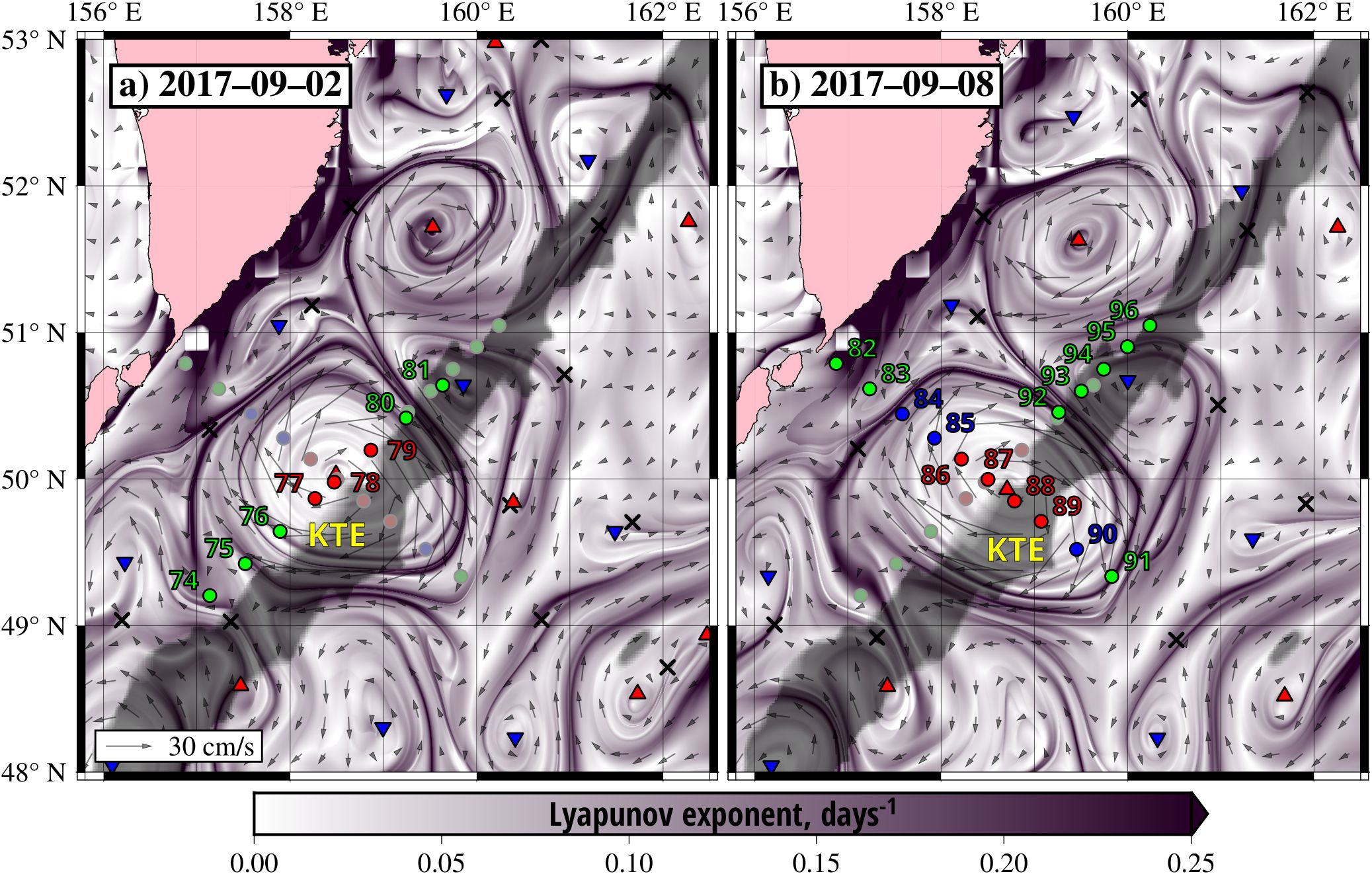
Figure 1. The altimetry-based backward-in-time FTLE maps in the area of a Kamchatka quasi-stationary anticyclonic eddy in September of 2017 with the superimposed locations of the numbered sampling stations on (a) September 2 and (b) September 8 (Prants et al., 2020) and locations of the elliptic (red triangles for anticyclones, blue ones for cyclones) and hyperbolic points (crosses). The stations in the center of the eddy and at its periphery are indicated by red and blue circles, respectively. The green stations are located in surrounding waters.

Similar verification of these null-dimensional objects has been carried out with the Bussol mesoscale eddies (Prants et al, 2016), Hokkaido eddies (Prants et al, 2018), Kuroshio rings (Budyansky et al, 2015), the frontal eddies in the Japan Sea (Budyansky et al, 2024), the rings in the South Atlantic (Moroszov et al., 2022) and eddies in the Fram Strait (Sandalyuk et al., 2024). In all the cases, the elliptic points approximated locations of the centers of mesoscale eddies with the accuracy of the order of 5–10 km, that is better than the nominal resolution of the altimetry data due to smoothness of the velocity field inside eddies.

3.2 Hyperbolic points and associated invariant manifolds

Hyperbolic points in DST have associated stable $W_s$ and unstable $W_u$ manifolds which strongly influence motion in chaotic systems. In fluid flows, the stable and unstable invariant manifolds are 1-D or 2-D surfaces in 3-D flows or 1-D lines in 2-D flows that consist of a collection of points through which at time moment t trajectories of those fluid elements pass that are asymptotic to that point at $t\to \infty$ and at $t\to - \infty$, respectively. Figure 2 shows the evolution of two compact tracer patches, located initially on both sides of the stable manifold. The patches deform over time and stretch along the unstable manifold, but the tracer does not cross the unstable manifold due to purely advective processes.

Figure 2

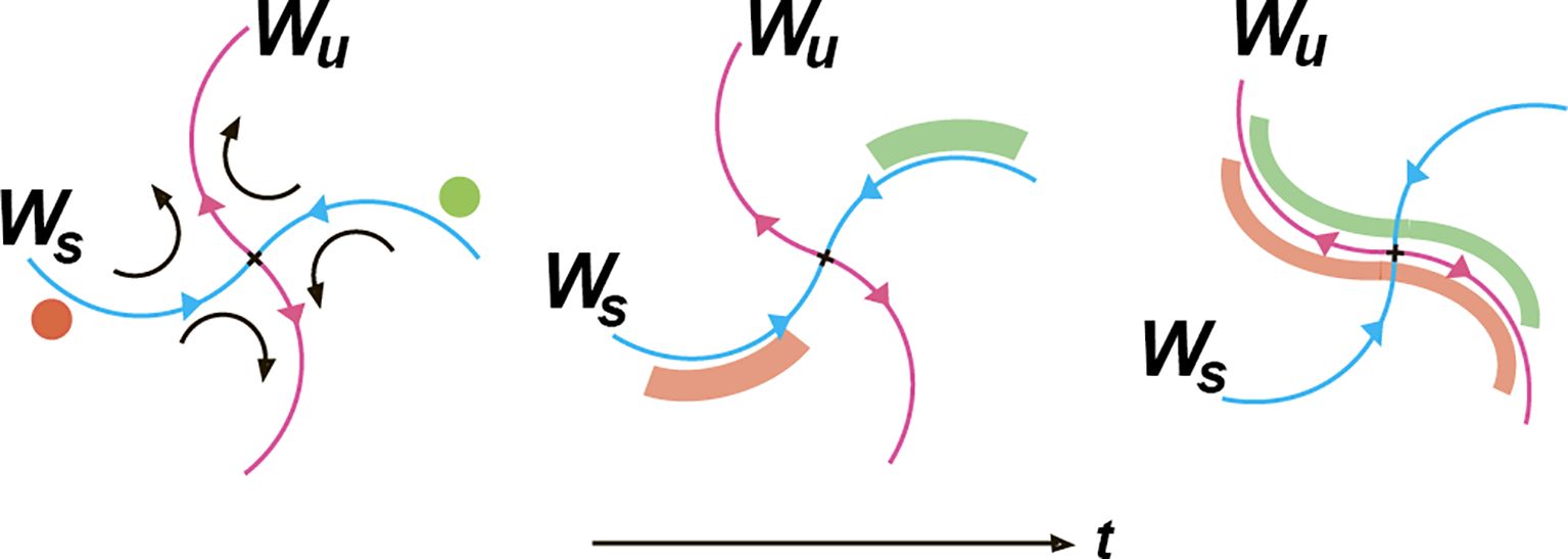
Figure 2. The advective evolution of two tracer patches in a vicinity of the hyperbolic point (cross) with the stable $W_s$ and unstable $W_u$ manifolds evolving in time. In the course of time (from a–c), the patches stretch along the unstable (attracting) manifold acting as a transport barrier.

The common way to detect stable (repelling) and unstable (attracting) manifolds is to calculate FTLE or FSLE fields on a grid. The lines with the maximum FTLE/FSLE values (‘ridges’), computed forward in time (${\Lambda }_{+}$), and backward-in time (${\Lambda }_{-}$), approximate locations of the most influential stable and unstable manifolds. The example is shown in Figure 3 in the area to east off the Kuril Islands (northwestern Pacific), where ${\Lambda }_{+}$ and ${\Lambda }_{-}$ ridges cross each other at hyperbolic points (crosses). The verification of simulated locations of hyperbolic points in the oceanic flows is more problematic than that for elliptic points. Their locations can be sometimes verified by trajectories of surface or subsurface floats with a specific behavior in the vicinity of hyperbolic points. As far as we know, the first observation of the presence of a hyperbolic point in the ocean occurred with the help of acoustically tracked RAFOS floats. The trajectories of 5 isopycnal RAFOS floats, drifting at the depth of around of 700 m in the Atlantic Ocean (Figure 4, Rossby et al., 1986), indicate the presence of stable (floats # 64 and 65) and unstable (floats # 57 and 63) manifolds associated with a hyperbolic point (float # 62).

Figure 3

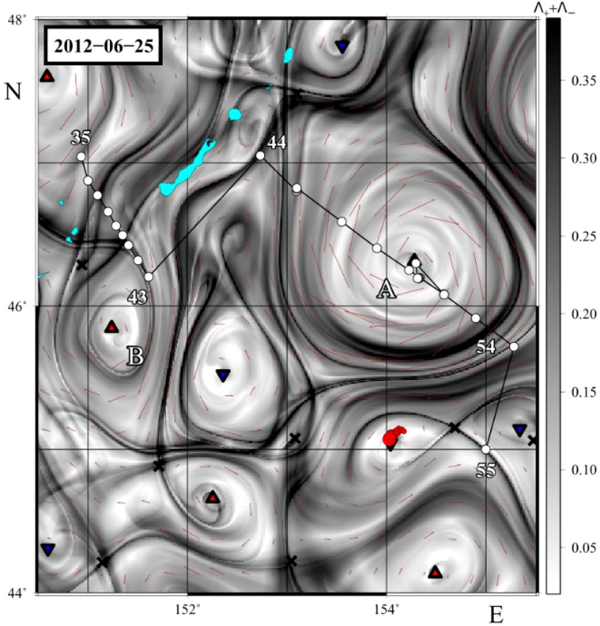
Figure 3. The combined altimetry-based forward- and backward-in time FTLE map in the area near a quasi-stationary Bussol eddy (A) in the northwestern Pacific sampled in June, 2012 by Prants et al., 2016. The light blue spots are Kuril islands. In the days of sampling, this eddy formed a tripole structure with the anticyclone B and a cyclone between them. The black ridges with the (locally) maximum values of ${\Lambda }_{+}$ and ${\Lambda }_{-}$ approximate locations of the influential stable and unstable manifolds. The red and blue triangles indicate centers of anticyclones and cyclones, resp. The hyperbolic points are shown by crosses. Locations and numbers of sampling stations are shown by open circles. The red full circles are locations of surface drifters for a few days before and after June, 25. The values of ${\Lambda }_{-}$ in ${\text{days}}^{-1},$ computed backward in time for a month, are coded by nuances of the grey color.

Figure 4

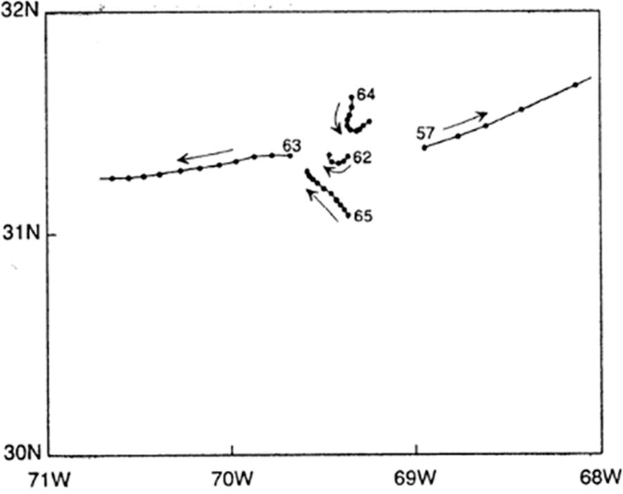
Figure 4. Trajectories of five isopycnal RAFOS floats drifting at the depth of around of 700 m in the Atlantic indicating the presence of stable (floats # 64 and 65) and unstable (floats # 57 and 63) manifolds associated with a hyperbolic point (float # 62) (courtesy of T. Rossby).

A number of observations of the presence of hyperbolic points have been done with surface drifters. Trajectories of two surface drifters in the Pacific Ocean are shown in Figure 5. The drifters approach a hyperbolic point along its stable manifold and then move away along the unstable manifold calculated in the altimetry-based FTLE field (Prants et al, 2016). After approaching the hyperbolic point, one float turned west and entered the Okhotsk Sea, and another one turned to east into the open ocean. The influence of hyperbolic points has been also observed in tracks of drifters deployed in June 2011 and by Nishikawa et al. (2021) in August 2017 in the Kuroshio-Oyashio frontal zone. The launching of floats in the vicinity of hyperbolic points provides valuable information about the circulation, transport and mixing (see Sec. 10).

Figure 5

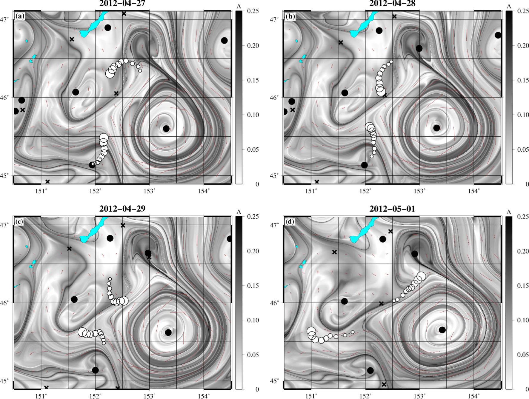
Figure 5. The altimetry-based FTLE maps in the area of the Kuril Islands in northwestern Pacific Ocean with the superimposed locations of two surface drifters (open circles) with the size of circles increasing in time. The drifters approach the calculated hyperbolic point (cross at 46°N, 152.4°E) along its stable manifold (a, b) and then move away from it along the unstable manifold (c, d). The locations of the elliptic points are shown by the filled circles. The Λ values are given in ${\text{days}}^{-1}$.

4 Lagrangian structures and their sensitivity to imperfections of velocity fields

Since chaotic trajectories are exponentially sensitive to small variations in initial conditions, their direct interpretation is difficult. The fruitful idea is to search for robust coherent structures, the most influential manifolds, that ‘attract’ and ‘repel’ nearby fluid elements with the maximum rate compared with other manifolds. These distinguished features, called LCSs (Haller, 2001, 2002), exist for a finite time. The LCS are proxies of stable and unstable invariant manifolds (see Sec. 3). They are barriers preventing fluxes across them and dividing regions of qualitatively different dynamics (see Sec. 8). The locations of LCSs can be approximated calculating the FTLE/FSLE scalar fields on a grid (see Sec. 2). Recently, the concept of LFs has been introduced in order to identify and track frontal boundaries in the ocean (Prants et al., 2014a, b). The LF is defined as a line (surface in 3-D flows) of the (local) maximum gradient of a relevant LI. The LFs have the same advantages as LCS. However, in difference from LCS, abstract geometric objects of an associated dynamical system, the relevant LFs are proxies of fronts of real physical quantities that can be measured and observed (see Prants, 2022 for a discussion of the difference between LCSs and LFs and their connection with invariant manifolds).

The accuracy of Lagrangian calculations critically depends on the quality of the velocity field. The errors in the NCM output velocity fields are unavoidable because of incomplete knowledge of topography, coastline, wind forcing and lack of consideration of small-scale unresolved processes, whereas the altimetry data suffer from measurement errors, interpolation and different approximations. This results in amplification of errors in calculating trajectories. The important issue is to estimate to which extent the Lagrangian structures are sensitive to resolution, interpolation, and measurement imprecisions. Haller (2002) analyzed this problem, comparing the model and ‘true’ analytical velocity fields, and showed that LCSs are robust to errors in the velocity fields, if they are strongly attracting or repelling and exist for a sufficiently long time. Though chaotic particle’s trajectories diverge exponentially from ‘true’ trajectories near a repelling LCS, the location of the LCS is not expected to be perturbed to the same degree, since errors spread along the LCS. A rigorous mathematical link between FSLEs and LCSs has been studied by Karrasch and Haller (2013) who have proven that a FSLE ridge, satisfying certain conditions, does signal a nearby ridge of a FTLE field, which, in turn, indicates location of a LCS under further conditions. Other FSLE ridges, violating the established conditions, are false positives for LCSs.

A few studies have been carried out to verify the sensitivity of LCSs to errors in the altimetric velocity field (Keating et al., 2011; Hernandez-Carrasco et al., 2011; Harrison and Glatzmaier, 2012; Ghosh et al., 2021; Badza et al., 2023). The locations of LCSs have been found to be relatively insensitive to both sparse spatial and temporal resolution and to the velocity-field interpolation method. A small noise, added to advection equations, typically does not change significantly locations of strong Lagrangian structures, but it leads to a blurring of these structures (see, e.g., Makarov et al., 2006; Hernandez-Carrasco et al., 2011; Harrison and Glatzmaier, 2012; Ghosh et al., 2021).

The comparison of altimetry-derived mesoscale Lagrangian structures with independent remote-sensing data, in situ measurements of thermal fronts, patterns of plankton blooms and with tracks of drifters and floats in different seas and oceans has shown a good correspondence (e.g., Abraham and Bowen, 2002; Beron-Vera et al., 2008; d’Ovidio et al., 2009; Hernandez-Carrasco et al., 2011; Prants et al., 2011a, b, 2017a; Huhn et al., 2012; Prants et al., 2014a and many others). In particular, the FTLE/FSLE diagnostics still give an accurate picture of the Lagrangian structures even if some dynamics are missed. However, submesoscale features are poorly resolved by the conventional altimetry data and should be considered with great caution (see Sec. 2). The launch of the SWOT mission (https://swot.jpl.nasa.gov/) at the end of 2022 opens up new opportunities in detecting smaller-scale Lagrangian structures and eddies compared with the conventional altimeters due to higher resolution of SWOT altimeters.

5 Limitations of the Lagrangian approach

The accuracy of the altimetry-based Lagrangian results is limited by the comparatively low spatial and temporal resolutions of the conventional altimetry data. The resolution of the order of 1/8°×1/8°for the global coverage and 1/12°×1/12° resolution in some regions enables to detect mesoscale features greater than ~ (30 – 50) km. In some cases, it is possible to identify submesoscale features in the tracer patterns that appear due to stirring and advection in a mesoscale field (e.g., Abraham and Bowen, 2002; Lehahn et al., 2007; d’Ovidio et al., 2009; Olascoaga and Haller, 2012; Prants et al., 2014a, 2016; Allshouse and Peacock, 2015; Fifani et al., 2021). The mesoscale stirring doesn’t mix water, but intensifies gradients at smaller scales. However, local submesoscale processes and features cannot be reproduced in conventional altimetry data.

Equation 1 is inherently nonlinear equation producing chaotic advection (Aref, 1984). This implies that particle trajectories can be exponentially sensitive to small variations in initial conditions even in regular Eulerian flows. The distance between initially close-by chaotic trajectories grows exponentially in time. As a consequence, it is impossible to forecast the particle position r beyond the so-called predictability horizon.

$${\tau }_p\approx \frac{1}{\text{Λ}}\ln \frac{{\text{Δ}}_r}{{\text{Δ}}_r(0)}$$

where ${\Delta }_r$ is a confidence interval, and ${\Delta }_r(0)$ is an inevitable inaccuracy in specifying initial particle’s position. The typical positive FTLE values of strong LCSs in the open ocean are in the range of 0.1 - 0.3 ${\text{days}}^{-1}$ (see Figures 2, 5) implying that the predictability horizon is, roughly, in the range of 3–10 days.

It is impossible to calculate ‘true’ chaotic trajectories in dynamically active regions. Can we trust the particle-tracking results in these regions (see Sec. 6)? This question deserves further consideration both from mathematical and oceanographic points of view. One of the arguments in favor of the particle-tracking results follows from the shadowing theorem in DST (see, e.g., Hammel et al., 1987). The theorem states that every numerically computed trajectory of a chaotic system stays close to the ‘true’ trajectory with a slightly altered initial position. In other words, a pseudo-trajectory is ‘shadowed’ by a true one. This suggests that the particle-tracking numerical experiments with a sufficiently large massive of particles can be trusted to represent the real movement of water masses.

6 Lagrangian transport

Starting from the middle of 90s, LA is an active area of research to study tracer transport pathways where a patch of tracer (heat, salt, nutrients or radionuclides) is considered as a collection of virtual particles (Berloff and McWilliams, 2002; Wiggins, 2005; Griffa et al., 2009, 2013; Rypina et al., 2012; Prants et al., 2017a; van Sebille et al., 2018 and many others). Since the number of physical drifters in the ocean is currently limited, the Lagrangian simulation provides an alternative way to study transport of water masses, detection of connectivity between different parts of the oceans, cross-shelf transport, fresh water and suspended material transport in river mouths, predicting the location of missing objects, the movement of fish larvae and plankton, particle dispersion, the spread of pollution, etc.

Two main approaches are used to add diffusion to trajectories and to account for unresolved physics. One is to use the tracer concentration equation in the form of a Fokker–Planck equation which describes the time evolution of the probability density function of the tracer. The Markov models are used in the second approach to fit to observations from surface drifter trajectories or virtual particles in a much finer resolution velocity field. The reader is referred to Griffa et al. (2009) and van Sebille et al. (2018), who reviewed these approaches in detail. The applicability of the stochastic simulations should be verified against existing observations or high-resolution model simulations. If a velocity field is available at sufficiently high spatial and temporal resolutions, adding a stochastic component may be unnecessary and a large number of particles may suffice (Koszalka et al., 2013).

Several online and offline particle-tracking software packages are available to simulate 3-D water-parcel pathways in NCMs: TRACMASS (https://www.tracmass.org, Doos, 1995), Larval TRANSport Lagrangian model (LTRANS, https://github.com/LTRANS/LTRANSv.2b, North et al., 2008), OceanParcels project (http://oceanparcels.org. They can be used to simulate trajectories of passive and active particulates such as plankton, microplastic and larvae.

The performance of the particle-tracking experiments depends on the specific task. When simulating the transport pathways of water masses and the connectivity between different parts of the ocean or between the oceans, the Lagrangian particles are tagged and then followed until they reach the certain domain. If the task is to estimate a fraction of different water types or water masses in a certain basin, it is required to partition the basin by subdividing it into a large number of small bins. The particles are integrated backward in time until they reach certain regions which are supposed to be the sources of specific water masses. In tracer studies, the tracer is tracked through the velocity fields to estimate its dispersion.

Different water masses often converge and mix in the frontal zones and in some basins. The fraction of each water mass on a given date can be inferred from the trajectories of Lagrangian particles integrated in reverse time until they reach the segments that are supposed to cross the transport pathway of a certain water mass. The integration time is determined empirically and should be enough long for particles to reach the study area from remote places. Each trajectory is stopped when it reaches the chosen segments, and the locations of particles are depicted by color on the geographic map creating an origin map on a specific date (Prants et al., 2018). Each color on such maps represents the specific water mass. The gallery of the consecutive origin maps allows us to estimate intra- and interannual variations of the content of different water masses in a study area. As an example, Figure 6 shows the distribution of three water masses in the Okhotsk Sea, the largest marginal sea in the Pacific Ocean, connected to the subarctic gyre through the Kuril Straits and with the Japan Sea by a narrow strait, through which transformed subtropical water flows into the sea. The trajectories of 547,200 particles were calculated backward in time for one year until the trajectories reached one of the black segments in Figure 6, which were chosen to cross the transport pathways of the main water masses. This technique can also be applied to estimate the daily fractions of water of different origin within the surface cores of moving mesoscale eddies (Udalov et al., 2023, 2024).

Figure 6

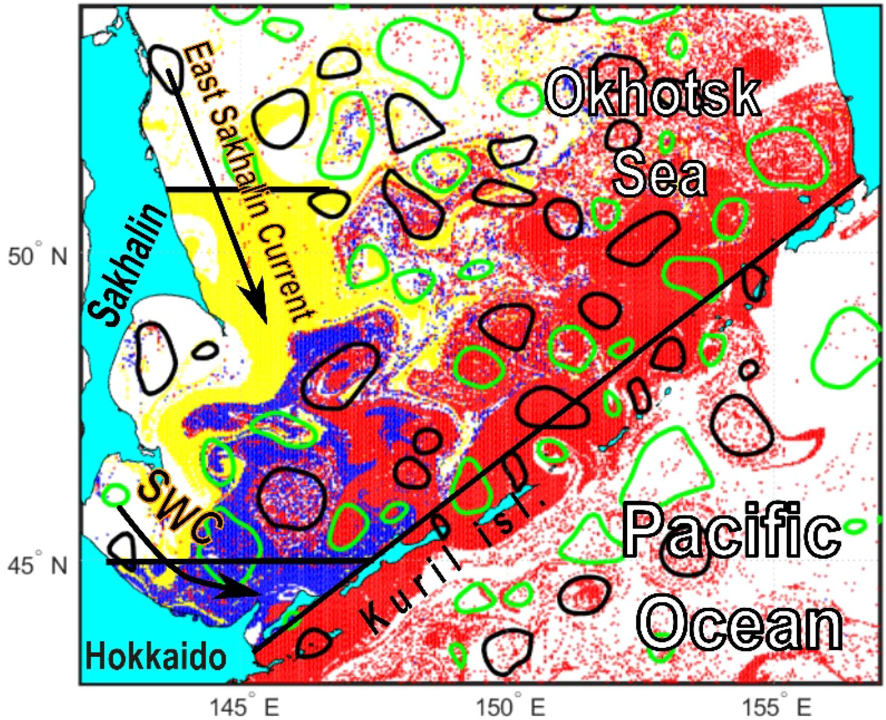
Figure 6. The altimetry-based origin map on December 27, 2021 shows distribution of three water masses in the Okhotsk Sea and adjacent area. The red color marks the particles which crossed for a year in the past the diagonal segment from the ocean side, the yellow and blue colors mark the East Sakhalin Current and Soya Warm Current (SWC) waters crossing the respective zonal segments. The contours of the detected mesoscale anticyclones (black ones) and cyclones (green ones) are shown on the same date. The white areas correspond to those particles which either did not cross one of the selected segments or because one year was not long enough to do that.

Tracking of virtual particles is commonly used to quantify connectivity between different regions assigning a volume transport value to each particle equal to the local velocity in the grid cell times the area of that cell (Doos, 1995; Speich et al., 2002; van Sebille et al., 2010, 2018). Many marine organisms reproduce with larvae advected by currents. It is important in marine ecology to estimate the larval exchange of a species between geographically separated sub-populations (Cowen and Sponaugle, 2009; Harrison et al., 2013; Puckett et al., 2014, 2014; Rossi et al., 2014).

Plumes of fresh water from big rivers spread over a large distance in the ocean with a great impact on the ocean dynamics. For example, the Amazon River plume strongly affects the regime of the entire equatorial Atlantic Ocean, reducing surface salinity and mixing by forming transport barriers far as 4000 km from the river mouth (Jo et al., 2005). Morozov et al. (2024) have carried out shipborne measurements and Lagrangian modeling of the advection of passive markers simulating freshwater parcels. Figure 7 shows the tracks of two patches with markers integrated backward in time. Their initial positions were selected at the sites and at times where and when, according to the measurements, the low-saline water has been detected. In both cases, the markers propagated backward in time coherently following the North Equatorial Countercurrent and North Brazil Current. However, their pathways differ, due to a high variability of circulation in the study region determined by meandering of the North Equatorial Countercurrent jet. This study provided a validation of the Lagrangian particle-tracking approach in finding the sources of freshwater far away from the discharge site. Different NCMs, satellite MODIS images and drifters have been used to track the Lagrangian particles and to verify the adequacy and accuracy of the LA to capture river plumes. The last but not least, transport of plastic has received a lot of efforts in the last years (see, e.g., Lebreton et al., 2012; Lohmann and Belkin, 2014; Miron et al., 2021 and many others.).

Figure 7

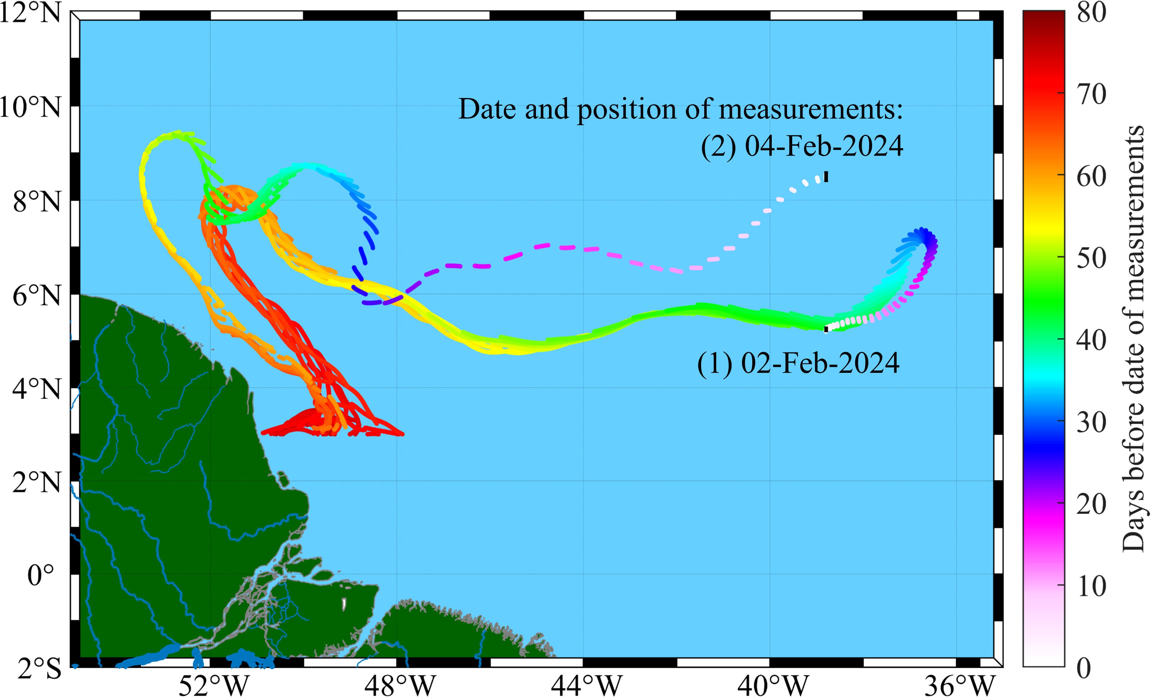
Figure 7. Composition of traces of trajectories of passive markers selected at the sites with the minimum salinities measured on 2^nd and 4^th February, 2024. The trajectories were calculated backward in time over 180 days based on the AVISO velocity field. The initial locations of the tracers are indicated by black. After reaching the zonal line along 3°N near the Amazon River mouth, the trajectories have not been calculated. The travelling time in days before the dates of measurements are given on the right (with the permission from Morozov et al., 2024).

7 Lagrangian identification of eddies

Eddies significantly contribute to the kinetic energy in the oceans with strong impact on weather and marine life, transporting salt, heat, nutrients, biota and pollutants sometimes over hundreds of kilometers away from the places of formation (see, e.g., Beron-Vera et al., 2008; Chelton et al., 2011; Dong et al., 2014; Budyansky et al., 2015; Prants, 2021a; Xia et al., 2022; Ueno et al., 2023; Liu and Abernathey, 2023; Udalov et al., 2023, 2024). Isolated mesoscale eddies consist of a vortex core and periphery separated by a transport barrier. The core is a coherent, but deforming feature, that retains the water properties for some time. The water on periphery rotates around the eddy’s center and exchanges with the surrounding. The boundary of the core of coherent eddies in oceanic flows retains its shape without significant stretching, folding and filamentation unlike a typical closed material line in chaotic flows. The Eulerian methods to detect and track mesoscale eddies use subjective thresholds like the Okubo-Weiss parameter, closed contours of sea level anomalies and others (e.g., Chelton et al., 2011; Le Vu et al., 2018). These methods cannot objectively determine the vortex-core boundaries. The majority of Lagrangian methods, based on calculation of FTLE/FSLE and other LIs, are also unable to objectively determine the core boundaries, since they do not provide us with a mathematical criteria for this determination. Haller and Beron-Vera (2012) and Haller et al. (2016) proposed the method for accurate detecting the boundaries of the vortex cores. This boundary is defined as the outermost closed contour of the Lagrangian-averaged vorticity deviation that can be calculated from the trajectory data (Wang et al., 2015; Abernathey and Haller, 2018; Xia et al., 2022; Liu and Abernathey, 2023). Numerous in situ observations and remote sensing often indicate higher chl-a concentrations and remarkable enhancements in biomasses at the boundaries of mesoscale eddies (e.g., Kusakabe et al., 2002; Xu et al., 2019; Zhang and Qiu, 2020; Zhao et al., 2021). The boundaries of some eddies are composed of productive water which is wrapped around the vortex core creating a high-productive belt.

8 Lagrangian transport barriers and their significance in pollution issues

The transport barriers are formally defined as material surfaces with zero transverse flux (Boffetta et al., 2001; Budyansky et al., 2009; Haller and Beron-Vera, 2012; Haller et al., 2016). However, this definition is not operationally useful, because the normal flux across any material surface in fluid flows is zero. The detection of transport barriers in oceanic flows is a challenge, because they are aperiodic and defined on finite space-time grids. The transport barriers have been operationally defined as exceptional material surfaces (lines) that deform less than their neighbors (Haller and Beron-Vera, 2012). The hyperbolic transport barriers in chaotic flows are associated with hyperbolic points. The ‘effective’ stable and unstable manifolds of these points (see Sec. 3 and Figures 3, 4) exist for a finite period of time, because the hyperbolic points in the ocean are of a transient nature.

In this section, we illustrate the significance of transport barriers in the spread of oil and dispersal of radionuclides after some accidents in different regions. Marine oil disasters occur more and more frequently (www.itopf.com/knowledge-resources/data-statistics/statistics) requiring immediate and effective response. The particle tracking (see Sec. 6) is used to simulate the spread of oil spills in order to find transport pathways retrospectively or in near-real time (see, e.g., Varlamov et al., 1999; Korotenko et al., 2004; Liu et al., 2011; Ono et al., 2013; Qiao et al., 2019; Prants, 2023). As the barrier moves, the tracer spreads along it because it plays the role of an attractive invariant manifold (see Sec. 3 and Figure 3). The FTLE/FSLE diagnostics and other LIs have been applied to locate the barriers in the dispersal of oil spills after catastrophic accidents in the Gulf of Mexico in 2010 (Olascoaga and Haller, 2012; Duran et al., 2018), in the East China Sea in 2018 (Qiao et al., 2019; Pan et al., 2020), in the Mediterranean Sea in 2021 (Fifani et al., 2021) and in other places.

To illustrate this issue, we discuss briefly the results on simulation of a hypothetical oil spill from the Kozmino terminal at the coast of the Peter the Great Bay (Japan Sea) using ROMS with the horizontal resolution of 600 m and assimilation of real hydrological and meteorological parameters (Prants, 2023). The model takes into account biodegradation and evaporation processes removing part of oil from the spill. In the warm season with prevailing southeasterly winds, the typical scenario of the dispersal of the oil slick is illustrated in Figures 8a, b with the FTLE field calculated backward in time following eq. 3. The strong barrier appears near the coast just after the launching of oil particles. It evolves in time, stretches the oil slick and blocks its removal offshore with a high risk for contamination of the bay (Figure 8b). The spread of spilled oil is cardinally different in the cold season when winds blow from the continent. The configuration of the transport barriers facilitates the spread of oil offshore stretching the slick along the most influential ones (Figures 8c, d).

Figure 8

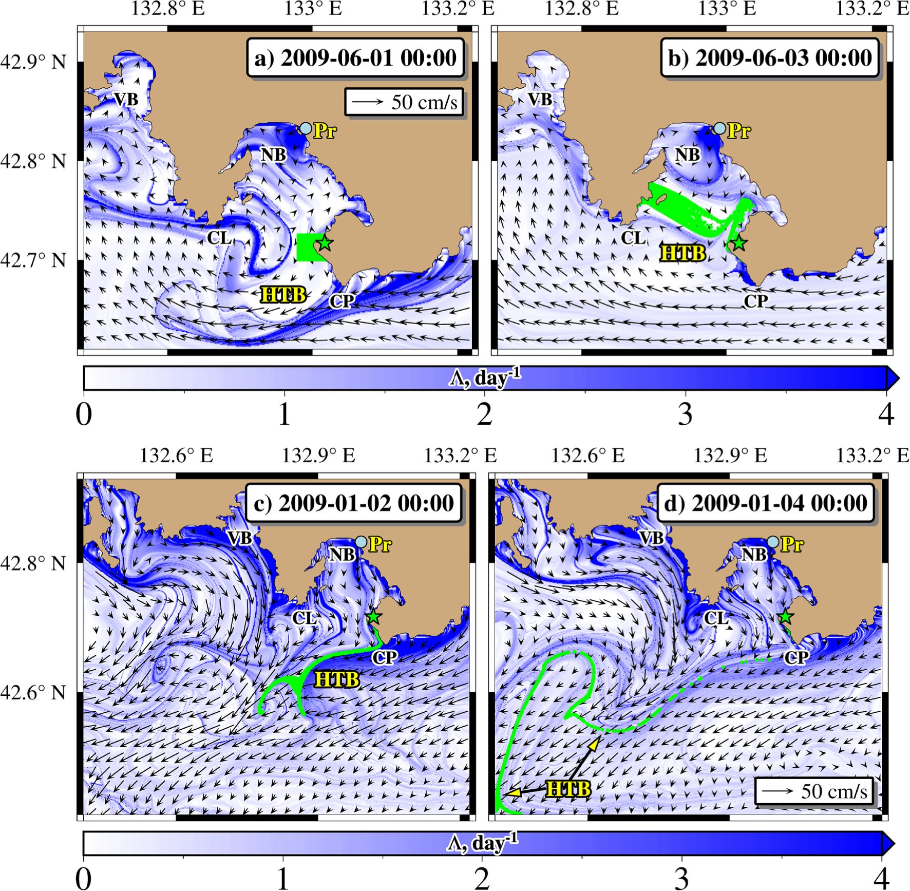
Figure 8. The ROMS surface velocity field with the superimposed FTLE values. (a, b) The spilled oil (green particles) deployed at the Kozmino oil terminal* on June 1^st, 2009 in the warm season typically remains near the coast. The coastal hyperbolic transport barriers (HTB) prevent offshore spread of oil. (c, d) In the cold season, the spilled oil typically disperses offshore and spreads along the evolving FTLE ridge approximating location of the influential HTB. SB, VB and NB are Strelok, Vostok and Nakhodka bays; CL and CP are Likhachev and Povorotny capes; Pr is the mouth of the Razdolnaya river.

The oil spills accidents require immediate response that ideally requires information on location of barriers and potential transport pathways in the area. However, the barriers evolve in time, sometimes in a complicated manner, as it is illustrated in Figure 8. The possibility to anticipate the location of the barriers, even for a short time, would be very important to forecast the spread of oil slicks. The Lagrangian diagnostics could help with this task allowing us to predict the location of the influential barriers. The point is that it can be done for a few days based only on the current velocity data without a velocity forecast.

Lagrangian simulation of the dispersal of radionuclides in the ocean started right after the accident at the Fukushima Nuclear Power Plant on March 11^th, 2011 based on altimetry and NCM velocity fields (Prants et al., 2011b; Tsumune et al., 2012; Kaeriyama et al., 2013; Rossi et al., 2013; Budyansky et al., 2015; Prants et al., 2014b, 2017b and many others). In particular, it has been shown that the contaminated water could be trapped by mesoscale eddies for a long time (Prants et al., 2011b, 2014b; Budyansky et al., 2015; Prants et al., 2017b). A year and half after the accident, increased concentration of the main radionuclides, $C{s}^{134}$ and $C{s}^{137},$ has been found in the cores of some anticyclonic mesoscale eddies at the depths ranging from 100 to 500 m (Budyansky et al., 2015). The barriers around the mesoscale eddies prevented the release of contaminated water out of the vortex cores facilitating the subduction of this water to intermediate depth.

Recently, the significance of hyperbolic transport barriers in the dispersal of radioactive material has been investigated after a little-known accident occurred on August 10^th, 1985 in the small Chazhma Bay (Peter the Great Bay, Japan Sea). The thermal explosion of the nuclear submarine reactor has been accompanied by radioactive pollution of seawater and air. The potential transport pathways at different depths have been retrospectively simulated for the first time using hourly velocity field output from the ROMS model with the horizontal resolution of 600 m (Budyansky et al., 2022a). The FTLE ridges in Figure 6 by Budyansky et al. (2022a) approximated location of the transport barriers in the area. The barriers around identified eddies in the study area prevented penetration of the contaminated water into the vortex cores during the lifespan of these eddies. The presumably radioactive particles have followed the attractive manifolds and spread along them. That allows to make a forecast of the dispersal of radionuclides in the model velocity field after identification of the influential hyperbolic points, which can be distinguished by the maximum singular values σ of the evolution matrix in eq. 3.

9 Marine life and fishery at Lagrangian fronts

The LF is strictly defined in Sec. 4 as a line (surface in 3-D flows) of the (local) maximum gradient of a relevant LI. The finite-time Lyapunov exponents (3) and (4) belong to one class of LIs. Other LI classes are listed in Sec. 2. The locations of mesoscale LFs can be easily calculated in the altimetric velocity field, whereas NCMs with higher resolution are required to calculate locations of smaller-scale LFs. In dependence of the indicator chosen, LFs may approximate ocean fronts with strong gradients of hydrological parameters or transport barriers as it is demonstrated in Figure 8, where the LFs govern dispersal of oil slicks. In this section, we briefly discuss the significance of LFs for some aspects of marine life at ocean fronts (for a comprehensive review see, Prants, 2022 and Prants, 2024).

Detection of the ocean fronts requires in situ measurements at a dense grid of stations that is practically impossible on a global scale. Until recently, SST maps have been the only tool to detect fronts remotely. However, cloudiness, low SST contrasts in warm seasons, noise and low spatial resolution of some satellite products may hinder the detection of thermal fronts (Ullman and Cornillon, 2000; Miller and Christodoulou, 2014). The alternative method has been developed for capturing frontal features in near real time based on the extraction of LFs in chaotic oceanic flows (Prants et al., 2014a). Even if the frontal water masses are almost indistinguishable on SST infrared images because of a small contrast, the LFs can be identified on the maps of the gradients of relevant indicators in altimetry-derived velocity fields under any weather conditions allowing us to track different phases of the evolution of fronts: frontogenesis, frontolysis and disappearance of fronts. It is important for sustainable fisheries, because the potential feeding grounds can be distinguished among a variety of frontal zones in a study area (Prants, 2022).

The LFs are both Eulerian features, since they are frontal sections, and Lagrangian features, since they are gradient lines of the relevant LIs. The horizontal gradients of temperature and density at strong fronts and deformation of the converging water masses generate a flow with steeply inclined isopycnal surfaces and cause a vertical ageostrophic secondary circulation (Hoskins, 1982). Although this circulation occurs on a relatively small scale, it is an important process delivering nutrients to the depleted euphotic layer and promoting growth and accumulation of phytoplankton at fronts (see Figure 1 by Prants, 2022). Aggregation of phytoplankton at fronts is accompanied by abundance of zooplankton providing food for small pelagic fish and squid, attracting in turn large pelagic fish, seabirds and top predators. We just mention some references, where it has been shown that the feeding sites of seabirds (Della Penna et al., 2017), of elephant seals (Cotte et al., 2015) and fishing grounds of many species of pelagic fish (Prants et al., 2014a; Budyansky et al., 2017; Watson et al., 2018; Scales et al., 2018; Prants et al., 2021b; Baudena et al., 2021; Budyansky et al., 2022b; Kulik et al., 2022; Díaz-Barroso et al., 2022) were not distributed randomly, but concentrated in the vicinity of the FTLE/FSLE ridges and LFs. Long-term retrospective calculation of the relevant LFs may be useful in obtaining a representative picture of the distribution of fronts in different seas and oceans along with the estimates of their persistence and spatio-temporal variability. That could help in making decisions in establishing marine protected areas around the frontal zones with a high level of bioproductivity and biodiversity.

10 Field experiments with Lagrangian drifters

In this section, we review briefly some targeted experiments with the surface drifters that have been conducted with the following purposes: (1) comparison of trajectories of drifters with numerically obtained trajectories in order to test the skill of particle trajectories in NCMs; (2) investigation of the circulation in a study area including meso- and submesoscale features; (3) dispersion studies; (4) Lagrangian data assimilation and validation of regional NCMs (Molcard et al., 2003, 2006; van Sebille et al., 2009; Huhn et al., 2012; Griffa et al., 2013).

The ensemble particle dispersion and the diffusivity are the Lagrangian metrics which directly relevant to spreading (see, e.g., Rypina et al., 2012) and clustering of floating tracers (see, e.g., Koshel et al., 2019; Meacham and Berloff, 2023, 2024, 2025). The studies have been carried out with drifters launched in pairs and triplets separated by a small distance giving information on relative dispersion at scales ranging from the submesoscale to mesoscale (LaCasce, 2008; Lumpkin and Elliot, 2010; Griffa et al., 2013). The extensive field campaigns with large groups of accurately tracked surface drifters, the Grand Lagrangian Deployment in July, 2012 (GLAD; Olascoaga et al., 2013; Poje et al., 2014) and the Lagrangian Submesoscale Experiment in January–February, 2016 (LASER; Haza et al, 2018; D’Asaro et al., 2018), have been conducted in the Gulf of Mexico. These experiments gave more accurate placement of frontal positions, directions and speed of currents and quantification of the submesoscale-driven dispersion missing in the current NCM and altimeter-derived velocity fields.

The DST and LA help to find the sites where preferably to launch drifters to get a valuable information about the circulation, transport and mixing. Several studies have been devoted to developing optimal drifter-launch strategies (Lumpkin et al., 2016) for Lagrangian data assimilation using locations of hyperbolic points, hyperbolic trajectories and the associated manifolds (Poje et al., 2002; Molcard et al., 2006; Salman et al., 2008). The launching of drifters near distinguished hyperbolic points provides optimal sampling with respect to other launching schemes, such as homogeneous coverage of a study area or randomly located initial deployments (Ide et al., 2002; Poje et al., 2002; Molcard et al., 2006). The launch of drifters in a vicinity of hyperbolic points allows them to pass a longer way moving along stable and unstable manifolds (see Figures 4, 5). While moving, such drifters could sample regions with different energetics. On the one hand, the drifters slow down nearby hyperbolic points due to the presence of saddle traps there (Uleysky et al., 2007). On the other hand, their kinetic energy is high when moving away from hyperbolic points along the associated unstable manifolds (Poje et al., 2002; Molcard et al., 2006). Moreover, release of drifters nearby hyperbolic points allows us to study high dispersion.

These field campaigns used not only Lagrangian buoys but also pioneered the coordinated use of aerial vehicles (manned aircrafts and relatively low cost aerostats and commercial drones) for remote sensing of inexpensive and biodegradable surface drifters such as bamboo plates (Carlson et al., 2018; D’Asaro et al., 2020). A new technique was developed to measure fine-scale ocean current gradients and other characteristics from the remote-sensing data. This technique has proved to be effective in spanning the wide range of space and time scales, from seconds and centimeters to weeks and degrees, covering the range of submesoscale and mesoscale motions, surface waves and boundary layer. The multiscale observations demonstrated the presence of motions on scales of 100 m to 20 km, including enhanced horizontal dispersion, unexpectedly strong horizontal convergence and vertical velocity and the concentration of surface materials due to submesoscale motions. These data, along with high-resolution models, have established the importance of submesoscale motions in the transport and fate of buoyant material in the near-surface layer.

The GPS-equipped fish-aggregating devices are widely used in tuna fisheries (Imzilen et al., 2019; Amemou et al., 2020). They also give information on near-surface currents. More than 100,000 devices are currently drifting around the globe. Their average lifespan at sea, 40 days, is much shorter than a typical drifter’s lifespan, 450 days, but these devices are much cheaper and numerous. It has been found by Imzilen et al. (2019), based on millions of position data from more than 15,000 fish-aggregating devices and 2,000 drifters, that the surface velocity components of these devices and surface drifters highly correlate in the tropical areas of Atlantic and Indian Oceans, where the purse seine fleets operate.

11 Some conclusions and perspectives of the Lagrangian approach

The Lagrangian structures demonstrate some robustness against velocity uncertainties when calculating their locations in real oceanic flows (Secs. 3 and 4). However, minimizing data uncertainty remains a challenge. The launch of the SWOT mission in 2022 (https://swot.jpl.nasa.gov) opens up new opportunities in increasing the quality of altimetric velocity fields due to higher resolution, especially, near coasts, compared with the conventional altimeters. SWOT data, after careful editing and processing, will provide information on submesoscales (Fu et al., 2024). The arsenal of the developed Lagrangian methods is SWOT-ready to provide us with unprecedented ‘ground truth’ on a more precise estimate of sea level elevation, geostrophic currents, vorticity and strain. The progress in development of NCMs and reanalyses with increased resolution and data assimilation give hope for improvement of the particle-tracking modelling and understanding the role of fine-scale circulation.

The verification of simulation results remains an important issue. Besides the commonly used tools, like high-resolution SST and altimetry data, ocean color images, profiling float’s and surface drifter’s data, ‘the old-fashioned’ ones, such as ship-board and mooring observations, still remain on the agenda. Launching big groups of surface drifters and using the GPS-equipped fish-aggregating devices could help in the verification and validation of NCMs and detection of Lagrangian structures. The LA already has proven to be successful in some ecological studies including understanding of the feeding strategy of sea creatures and sustainable fishery.

The application of DST to study 3D phenomena is in the initial stage of implementation. Some DST ideas and methods, used to study 2D flows, can be generalized to 3D flows. The point is that some 3D phenomena run at submesoscale, requiring data from NCMs and reanalyses for diagnostic of LCSs, transport barriers and LFs. Studying the link between horizontal mesoscale and vertical submesoscale circulations, as well as their influence on the advection of various tracers, is a complex problem. Submesoscale processes occur over relatively short timescales but have significant impact on marine ecosystems due to large gradients that cause vertical transport, facilitate the absorption of carbon dioxide, the delivery of nutrients to the euphotic zone and the removal of toxic waste products from it.

To detect 2D TBs, embedded in a 3D volume, the DST methods have been elaborated. One of the fruitful ideas is to define observed TBs as time-evolving material surfaces with extreme deformation on nearby sets of initial conditions (Blazevski and Haller, 2014). The 3D FSLE diagnostics has been applied to study 3D TBs in the Benguela and Iberian upwelling systems (Bettencourt et al., 2012, 2017, 2021) and to simulate permanent oxygen minimum zones in the region off Peru (Bettencourt et al., 2015). As to the new methods, machine learning and artificial intelligence could help in promoting the LA studies with big data.

Author contributions

SP: Writing – original draft, Writing – review & editing.

Funding

The author(s) declare that financial support was received for the research and/or publication of this article. The work was supported by the Russian Science Foundation (project no. 23-17-00068) with the help of a high-performance computing cluster at the Pacific Oceanological Institute (project no. 121021700341-2).

Conflict of interest

The author declares that the research was conducted in the absence of any commercial or financial relationships that could be construed as a potential conflict of interest.

Generative AI statement

The author(s) declare that no Generative AI was used in the creation of this manuscript.

Publisher’s note

All claims expressed in this article are solely those of the authors and do not necessarily represent those of their affiliated organizations, or those of the publisher, the editors and the reviewers. Any product that may be evaluated in this article, or claim that may be made by its manufacturer, is not guaranteed or endorsed by the publisher.

Abbreviations

DST, Dynamical systems theory; FTLE/FSLE, finite-time (scale) Lyapunov exponent; LA, Lagrangian approach; LCS, Lagrangian coherent structure; LF, Lagrangian front; LI, Lagrangian indicator; LM, Lagrangian map; NCM, numerical circulation model.

References

Abernathey R. and Haller G. (2018). Transport by lagrangian vortices in the eastern pacific. J. Phys. Ocean 48, 667–685. doi: 10.1175/JPO-D-17-0102.1

Crossref Full Text | Google Scholar

Abraham E. and Bowen M. (2002). Chaotic stirring by a mesoscale surface-ocean flow. Chaos 12, 373–381. doi: 10.1063/1.1481615

PubMed Abstract | Crossref Full Text | Google Scholar

Allshouse M. R. and Peacock T. (2015). Lagrangian based methods for coherent structure detection. Chaos: Interdiscip. J. Nonlinear Sci. 25, 097617. doi: 10.1063/1.4922968

PubMed Abstract | Crossref Full Text | Google Scholar

Amemou H., Koné V., Aman A., and Lett C. (2020). Assessment of a Lagrangian model using trajectories of oceanographic drifters and fishing devices in the Tropical Atlantic Ocean. Prog. Oceanogr 188, 102426. doi: 10.1016/j.pocean.2020.102426

Crossref Full Text | Google Scholar

Aref H. (1984). Stirring by chaotic advection. J. Fluid Mech. 143, 1–21. doi: 10.1017/S0022112084001233

Crossref Full Text | Google Scholar

Argo (2000). Argo float data and metadata from global Data Assembly Centre (Argo GDAC) (SEANOE). doi: 10.17882/42182

PubMed Abstract | Crossref Full Text | Google Scholar

Badza A., Mattner T. W., and Balasuriya S. (2023). How sensitive are Lagrangian coherent structures to uncertainties in data? Phys. D Nonlinear Phenom. 444, 133580. doi: 10.1016/j.physd.2022.133580

Crossref Full Text | Google Scholar

Baudena A., Ser-Giacomi E., D’Onofrio D., Capet X., Cotté C., Cherel Y., et al. (2021). Fine-scale structures as spots of increased fish concentration in the open ocean. Sci. Rep. 11, 15805. doi: 10.1038/s41598-021-94368-1

PubMed Abstract | Crossref Full Text | Google Scholar

Bennett A. F. (2006). Lagrangian Fluid Dynamics (Cambridge. UK: Cambridge University Press).

Google Scholar

Berloff P. S. and McWilliams J. C. (2002). Material transport in oceanic gyres. Part II: Hierarchy of stochastic models. J. Phys. Ocean. 32, 797–830. doi: 10.1175/1520-0485(2002)032<0797:MTIOGP>2.0.CO;2

Crossref Full Text | Google Scholar

Beron-Vera F. J., Olascoaga M. J., and Goni G. J. (2008). Oceanic mesoscale eddies as revealed by Lagrangian coherent structures. Geophys. Res. Lett. 35, L12603. doi: 10.1029/2008GL033957

Crossref Full Text | Google Scholar

Bettencourt J. H., Lopez C., and Hernandez-Garcia E. (2012). Oceanic three-dimensional Lagrangian coherent structures: A study of a mesoscale eddy in the Benguela upwelling region. Ocean Model. 51, 73–83. doi: 10.1016/j.ocemod.2012.04.004

Crossref Full Text | Google Scholar

Bettencourt J., López C., Hernández-García E., Montes I., Sudre J., Dewitte B., et al. (2015). Boundaries of the Peruvian oxygen minimum zone shaped by coherent mesoscale dynamics. Nat. Geosci 8, 937–940. doi: 10.1038/ngeo2570

Crossref Full Text | Google Scholar

Bettencourt J. H., Rossi V., Hernández-García E., Marta-Almeida M., and López C. (2017). Characterization of the structure and cross-shore transport properties of a coastal upwelling filament using three-dimensional finite-size Lyapunov exponents. J. Geophys. Res. Ocean. 122, 7433–7448. doi: 10.1002/2017JC012700

Crossref Full Text | Google Scholar

Blazevski D. and Haller G. (2014). Hyperbolic and elliptic transport barriers in three-dimensional unsteady flows. Phys. D Nonlinear Phenom. 273–274, 46–62. doi: 10.1016/j.physd.2014.01.007

Crossref Full Text | Google Scholar

Boffetta G., Lacorata G., Redaelli G., and Vulpiani A. (2001). Detecting barriers to transport: A review of different techniques. Phys. D Nonlinear Phenom. 159, 58–70. doi: 10.1016/S0167-2789(01)00330-X

Crossref Full Text | Google Scholar

Budyansky M. V., Fayman P. A., Uleysky M. Y., and Prants S. V. (2022a). The impact of circulation features on the dispersion of radionuclides after the nuclear submarine accident in Chazhma Bay (Japan Sea) in 1985: A retrospective Lagrangian simulation. Mar. pollut. Bull. 177, 113483. doi: 10.1016/j.marpolbul.2022.113483

PubMed Abstract | Crossref Full Text | Google Scholar

Budyansky M. V., Goryachev V. A., Kaplunenko D. D., Lobanov V. B., Prants S. V., Sergeev A. F., et al. (2015). Role of mesoscale eddies in transport of Fukushima derived cesium isotopes in the ocean, Deep Sea Res. Pt. I 96, 15–27. doi: 10.1016/j.dsr.2014.09.007

Crossref Full Text | Google Scholar

Budyansky M. V., Kulik V. V., Kivva K. K., Uleysky M. Yu., and Prants S. V. (2022b). Lagrangian analysis of pacific waters in the sea of okhotsk based on satellite data in application to the alaska pollock fishery. Izv. Atmos. Ocean. Phys. 58, 1427–1437. doi: 10.1134/S0001433822120088

Crossref Full Text | Google Scholar

Budyansky M., Ladychenko S., Lobanov V., Prants S. V., and Udalov A. (2024). Evolution and structure of a mesoscale anticyclonic eddy in the northwestern Japan sea and its exchange with surrounding waters: in situ observations and lagrangian analysis. Ocean Dyn. 74, 901–917. doi: 10.1007/s10236-024-01631-w

Crossref Full Text | Google Scholar

Budyansky M. V., Prants S. V., Samko E. V., and Uleysky M. Y. (2017). Identification and Lagrangian analysis of oceanographic structures favorable for fishery of neon flying squid (Ommastrephes bartramii) in the South Kuril area. Oceanology 57, 648–660. doi: 10.1134/S0001437017050034

Crossref Full Text | Google Scholar

Budyansky M. V., Uleysky M. Y., and Prants S. V. (2009). Detection of barriers to cross-jet Lagrangian transport and its destruction in a meandering flow. Phys. Rev. E 79, 56215. doi: 10.1103/PhysRevE.79.056215

PubMed Abstract | Crossref Full Text | Google Scholar

Carlson D. F., Özgökmen T., Novelli G., Guigand C., Chang H., Fox-Kemper B., et al. (2018). Surface ocean dispersion observations from the ship-tethered aerostat remote sensing system. Front. Mar. Sci. 5. doi: 10.3389/fmars.2018.00479

Crossref Full Text | Google Scholar

Chelton D. B., Schlax M. G., and Samelson R. M. (2011). Global observations of nonlinear mesoscale eddies. Prog. Oceanogr 91, 167–216. doi: 10.1016/j.pocean.2011.01.002

Crossref Full Text | Google Scholar

Cotte C., d’Ovidio F., Dragon A.-C., Guinet C., and Levy M. (2015). Flexible preference of southern elephant seals for distinct mesoscale features within the Antarctic Circumpolar Current. Prog. Oceanogr. 131, 46–58. doi: 10.1016/j.pocean.2014.11.011

Crossref Full Text | Google Scholar

Cowen R. K. and Sponaugle S. (2009). Larval dispersal and marine population connectivity. Ann. Rev. Mar. Sci. 1, 443–466. doi: 10.1146/annurev.marine.010908.163757

PubMed Abstract | Crossref Full Text | Google Scholar

D’Asaro E. A., Shcherbina A. Y., Klymak J. M., Molemaker J., Novelli G., Guigand M., et al. (2018). Ocean convergence and the dispersion of flotsam. Proc. Natl. Acad. Sci. U.S.A. 115, 1162–1167. doi: 10.1073/pnas.1802701115

PubMed Abstract | Crossref Full Text | Google Scholar

D’Asaro E. A., Carlson D. F., Chamecki M., Harcourt R. R., Haus B. K., Fox-Kemper B., et al. (2020). Advances in observing and understanding small-scale open ocean circulation during the gulf of Mexico research initiative era. Front. Mar. Sci. 7. doi: 10.3389/fmars.2020.00349

Crossref Full Text | Google Scholar

d’Ovidio F., Della Penna A., Trull T. W., Nencioli P., Pujol M.-I., Rio M.-H., et al. (2015). The biogeochemical structuring role of horizontal stirring: Lagrangian perspectives on iron delivery downstream of the Kerguelen Plateau. Biogeosciences 12, 5567–5581. doi: 10.5194/bg-12-5567-2015

Crossref Full Text | Google Scholar

d’Ovidio F., De Monte S., Della Penna A., Cotté C., and Guinet C. (2013). Ecological implications of eddy retention in the open ocean: a Lagrangian approach. J. Phys. A 46, 254023. doi: 10.1088/1751-8113/46/25/254023

Crossref Full Text | Google Scholar

d’Ovidio F., Fernandez V., Hernandez-Garcнa E., and Lopez C. (2004). Mixing structures in the Mediterranean Sea from finite-size Lyapunov exponents. Geophys. Res. Lett. 31, L17203. doi: 10.1029/2004GL020328

Crossref Full Text | Google Scholar

d’Ovidio F., Isern-Fontanet J., López C., Hernández-García E., and García-Ladona E. (2009). Comparison between Eulerian diagnostics and finite-size Lyapunov exponents computed from altimetry in the Algerian basin. Deep Sea Res. Pt. I 56, 15–31. doi: 10.1016/j.dsr.2008.07.014

Crossref Full Text | Google Scholar

Della Penna A., Koubbi P., Cotté C., Bon C., Bost C.-A., and d’Ovidio F. (2017). Lagrangian analysis of multi-satellite data in support of open ocean Marine Protected Area design. Deep Sea Res. Part II 140, 212–221. doi: 10.1016/j.dsr2.2016.12.014

Crossref Full Text | Google Scholar

Díaz-Barroso L., Hernandez-Carrasco I., Orfila A., Reglero P., Balbín R., Hidalgo M., et al. (2022). Singularities of surface mixing activity in the Western Mediterranean influence bluefin tuna larval habitats. Mar. Ecol. Prog. Ser. 685, 69–84. doi: 10.3354/meps13979

Crossref Full Text | Google Scholar

Dong C., McWilliams J. C., Liu Y., and Chen D. (2014). Global heat and salt transports by eddy movement. Nat. Commun. 5, 3294. doi: 10.1038/ncomms4294

PubMed Abstract | Crossref Full Text | Google Scholar

Doos K. (1995). Interocean exchange of water masses. J. Geophys. Res. 100, 13499–13514. doi: 10.1029/95JC00337

Crossref Full Text | Google Scholar

Duran R., Beron-Vera F. J., and Olascoaga M. J. (2018). Extracting quasi-steady Lagrangian transport patterns from the ocean circulation: An application to the Gulf of Mexico. Sci. Rep. 8, 5218. doi: 10.1038/s41598-018-23121-y

PubMed Abstract | Crossref Full Text | Google Scholar

Fifani G., Baudena A., Fakhri M., Baaklini G., Faugère Y., Morrow R., et al. (2021). Drifting speed of Lagrangian fronts and oil spill dispersal at the ocean surface. Remote Sens. 13, 4499. doi: 10.3390/rs13224499

Crossref Full Text | Google Scholar

Fu L. L., Pavelsky T., Crétaux J.-F., Morrow R., Farrar J.-T., Vaze P., et al. (2024). The Surface Water and Ocean Topography Mission: A breakthrough in radar remote sensing of the ocean and land surface water. Geophys. Res. Lett. 51, e2023GL107652. doi: 10.1029/2023GL107652

Crossref Full Text | Google Scholar

Griffa A., Haza A., Ozgokmen T., et al. (2013). Investigating transport pathways in the ocean. Deep Sea Res. P.II 85, 81–95. doi: 10.1016/j.dsr2.2012.07.031

Crossref Full Text | Google Scholar

Griffa, A., Kirwan Jr., A., Mariano, A., Ozgokmen, T., and Rossby, H. (Eds.) (2009). Lagrangian Analysis and Prediction of Coastal and Ocean Dynamics (Cambridge: Cambridge University Press, U.K). doi: 10.1017/CBO9780511535901

Crossref Full Text | Google Scholar

Haller G. (2001). Distinguished material surfaces and coherent structures in 3D fluid flows. Phys. D Nonlinear Phenom. 149, 248–277. doi: 10.1016/S0167-2789(00)00199-8

Crossref Full Text | Google Scholar

Haller G. (2002). Lagrangian coherent structures from approximate velocity data. Phys. Fluids 14, 1851–1861. doi: 10.1063/1.1477449

Crossref Full Text | Google Scholar

Haller G. (2015). Lagrangian coherent structures. Ann. Rev. Fluid Mech. 47, 137. doi: 10.1146/annurev-fluid-010313-141322

Crossref Full Text | Google Scholar

Haller G. and Beron-Vera F. J. (2012). Geodesic theory of transport barriers in two-dimensional flows. Phys. D Nonlinear Phenom 241, 1680–1702. doi: 10.1016/j.physd.2012.06.012

Crossref Full Text | Google Scholar

Haller G., Hadjighasem A., Farazmand M., and Huhn F. (2016). Defining coherent vortices objectively from the vorticity. J. Fluid Mech. 795, 136–173. doi: 10.1017/jfm.2016.15

Crossref Full Text | Google Scholar

Hammel S. M., Yorke J. A., and Grebogi C. (1987). Do numerical orbits of chaotic dynamical processes represent true orbits? J. @ Complexity 3, 136–145. doi: 10.1016/0885-064X(87)90024-0

Crossref Full Text | Google Scholar

Harrison C. S. and Glatzmaier G. A. (2012). Lagrangian coherent structures in the California Current System - sensitivities and limitations. Geophys. Astrophys. Fluid Dyn. 106, 22–44. doi: 10.1080/03091929.2010.532793

Crossref Full Text | Google Scholar

Harrison C. S., Siegel D. A., and Mitarai S. (2013). Filamentation and eddy– eddy interactions in marine larval accumulation and transport. Mar. Ecol. Prog. Ser. 472, 27–44. doi: 10.3354/meps10061

Crossref Full Text | Google Scholar

Haza A. C., D’Asaro E., Chang H., Chen S., Curcic M., Guigand C., et al. (2018). Drogue-loss detection for surface drifters during the Lagrangian Submesoscale Experiment (LASER). J. Atmos. Oceanic Technol. 35, 705–725. doi: 10.1175/JTECH-D-17-0143.1

Crossref Full Text | Google Scholar

Hernandez-Carrasco I., Lopez C., Hernandez-Garcia E., and Turiel A. (2011). How reliable are finite-size Lyapunov exponents for the assessment of ocean dynamics? Ocean Model. 36, 208–218. doi: 10.1016/j.ocemod.2010.12.006

Crossref Full Text | Google Scholar

Hoskins B. J. (1982). The mathematical theory of frontogenesis. Annu. Rev. Fluid Mech. 14, 131–151. doi: 10.1146/annurev.fl.14.010182.001023

Crossref Full Text | Google Scholar

Huhn F., von Kameke A., Perez-Muсuzuri V., Olascoaga M. J., and Beron-Vera F. J. (2012). The impact of advective transport by the South Indian Ocean Countercurrent on the Madagascar plankton bloom. Geophys. Res. Lett. 39, L06602. doi: 10.1029/2012GL051246

Crossref Full Text | Google Scholar

Ide K., Small D., and Wiggins S. (2002). Distinguished hyperbolic trajectories in time-dependent fluid flows: analytical and computational approach for velocity fields defined as data sets. Nonlin. Proc. Geophys 9, 237–263. doi: 10.5194/npg-9-237-2002

Crossref Full Text | Google Scholar

Imzilen T., Chassot E., Barde J., Demarcq H., Maufroy A., Roa-Pascuali L., et al. (2019). Fish aggregating devices drift like oceanographic drifters in the near-surface currents of the Atlantic and Indian Oceans. Progr. Oceanogr. 171, 108–127. doi: 10.1016/j.pocean.2018.11.007

Crossref Full Text | Google Scholar

Jo Y.-H., Yan X.-H., Dzwonkowski B., and Liu W. T. (2005). A study of the freshwater discharge from the Amazon River into the tropical Atlantic using multi-sensor data. Geophys. Res. Lett. 32, L02605. doi: 10.1029/2004GL021840

Crossref Full Text | Google Scholar

Kaeriyama H., Ambe D., Shimizu Y., Fujimoto K., Ono T., Yonezaki S., et al. (2013). Direct observation of 134Cs and 137Cs in surface sea water in the western and central North Pacific after the Fukushima Dai-ichi nuclearpower plant accident. Biogeosciences 10, 4287–4295. doi: 10.5194/bg-10-4287-2013

Crossref Full Text | Google Scholar

Karrasch D. and Haller G. (2013). Do Finite-Size Lyapunov Exponents detect coherent structures? Chaos 23, 043126. doi: 10.1063/1.4837075

PubMed Abstract | Crossref Full Text | Google Scholar

Keating S. R., Smith K. S., and Kramer P. R. (2011). Diagnosing lateral mixing in the upper ocean with virtual tracers: Spatial and temporal resolution dependence. J. Phys. Ocean. 41, 1512–1534. doi: 10.1175/2011JPO4580.1

Crossref Full Text | Google Scholar

Korotenko K., Mamedov R., Kontar A., and Korotenko L. (2004). Particle tracking method in the approach for prediction of oil slick transport in the sea: Modelling oil pollution resulting from river input. J. Mar. Syst. 48, 159–170. doi: 10.1016/j.jmarsys.2003.11.023

Crossref Full Text | Google Scholar

Koshel K. V. and Prants S. V. (2006). Chaotic advection in the ocean. Phys.-Usp. 49, 1151–1178. doi: 10.1070/PU2006v049n11ABEH006066

Crossref Full Text | Google Scholar

Koshel K. V., Stepanov D. V., Ryzhov E. A., Berloff P., and Klyatskin V. I. (2019). Clustering of floating tracers in weakly divergent velocity fields. Phys. Rev. E 100, 063108. doi: 10.1103/PhysRevE.100.063108

PubMed Abstract | Crossref Full Text | Google Scholar

Koszalka I. M., Haine T. W. N., and Magaldi M. G. (2013). Fates and travel times of Denmark Strait Overflow Water in the Irminger Basin. J. Phys. Oceanogr. 43, 2611–2628. doi: 10.1175/JPO-D-13-023.1

Crossref Full Text | Google Scholar

Kulik V. V., Prants S. V., Uleysky M. Y., and Budyansky M. V. (2022). Lagrangian characteristics in the western North Pacific help to explain variability in Pacific saury fishery. Fish. Res. 252, 106361. doi: 10.1016/j.fishres.2022.106361

Crossref Full Text | Google Scholar

Kusakabe M., Andreev A., Lobanov V., Zhabin I., Kumamoto Y., and Murata A. (2002). Effects of the anticyclonic eddies on water masses, chemical parameters and chlorophyll distributions in the oyashio current region. J. Oceanogr. 58, 691–701. doi: 10.1023/A:1022846407495

Crossref Full Text | Google Scholar

LaCasce J. H. (2008). Statistics from lagrangian observations. Progr. Oceanogr. 77, 1–29. doi: 10.5194/gmd-10-4175-2017

Crossref Full Text | Google Scholar

Lebreton L. C.-M., Greer S. D., and Borrero J. C. (2012). Numerical modelling of floating debris in the world’s oceans. Mar. pollut. Bull. 64, 653–661. doi: 10.1016/j.marpolbul.2011.10.027

PubMed Abstract | Crossref Full Text | Google Scholar

Lehahn Y., d’Ovidio F., and Koren I. (2018). A satellite-based Lagrangian view on phytoplankton dynamics. Ann. Rev. Mar. Sci. 10, 99. doi: 10.1146/annurev-marine-121916-063204

PubMed Abstract | Crossref Full Text | Google Scholar

Lehahn Y., d’Ovidio F., Lévy M., and Heifetz E. (2007). Stirring of the northeast Atlantic spring bloom: A Lagrangian analysis based on multisatellite data. J. Geophys. Res.: Oceans 112, C08005. doi: 10.1029/2006JC003927

Crossref Full Text | Google Scholar

Le Vu B., Stegner A., and Arsouze T. (2018). Angular momentum eddy detection and tracking algorithm (AMEDA) and its application to coastal eddy formation. J. Atmos. Ocean. Technol. 35, 739–762. doi: 10.1175/JTECH-D-17-0010.1

Crossref Full Text | Google Scholar

Liu T. and Abernathey R. (2023). A global Lagrangian eddy dataset based on satellite altimetry. Earth Syst. Sci. Data 15, 1765–1778. doi: 10.5194/essd-15-1765-2023

Crossref Full Text | Google Scholar

Liu Y., Macfadyen A., Macfadyen A., Ji Z.-G., and Weisberg R. H. (Ed.) (2011). Monitoring and Modeling the Deepwater Horizon Oil Spill: A Record Breaking Enterprise. 1st Edition (Washington, DC: American Geophysical Union). doi: 10.1029/GM195

Crossref Full Text | Google Scholar

Lohmann R. and Belkin I. M. (2014). Organic pollutants and ocean fronts across the Atlantic Ocean: A review. Progr. Ocean. 128, 172–184. doi: 10.1016/j.pocean.2014.08.013

Crossref Full Text | Google Scholar

Lumpkin R., Centurioni L., and Perez R. C. (2016). Fulfilling observing system implementation requirements with the global drifter array. J. Atmos. Ocean. Technol. 33, 685–695. doi: 10.1175/JTECH-D-15-0255.1

Crossref Full Text | Google Scholar

Lumpkin R. and Elliot S. (2010). Surface drifter pair spreading in the North Atlantic. J. Geophys. Res.: Oceans 115, C12017. doi: 10.1029/2010JC006338

Crossref Full Text | Google Scholar

Makarov D., Uleysky M., Budyansky M., and Prants S. (2006). Clustering in randomly driven Hamiltonian systems. Phys. Rev. E 73, 66210. doi: 10.1103/PhysRevE.73.066210

PubMed Abstract | Crossref Full Text | Google Scholar

Meacham J. and Berloff P. (2023). On clustering of floating tracers in random velocity fields. J. Adv. Model. Earth Sys 15, e2022MS003484. doi: 10.1029/2022MS003484

Crossref Full Text | Google Scholar

Meacham J. and Berloff P. (2024). Clustering as a mechanism for enhanced reaction of buoyant species. J. Mar. Syst. 243, 103952. doi: 10.1016/j.jmarsys.2023.103952

Crossref Full Text | Google Scholar

Meacham J. and Berloff P. (2025). Clustering of buoyant tracer in quasigeostrophic coherent structures. J. Fluid Mech. 1003, A16. doi: 10.1017/jfm.2024.1229

Crossref Full Text | Google Scholar

Miller P. I. and Christodoulou S. (2014). Frequent locations of oceanic fronts as an indicator of pelagic diversity: Application to marine protected areas and renewables. Mar. Policy 45, 318–329. doi: 10.1016/j.marpol.2013.09.009

Crossref Full Text | Google Scholar

Miron P., Beron-Vera F. J., Helfmann L., and Koltai P. (2021). Transition paths of marine debris and the stability of the garbage patches. Chaos 31, 033101. doi: 10.1063/5.0030535

PubMed Abstract | Crossref Full Text | Google Scholar

Molcard A., Piterbarg L., Griffa A., Özgökmen T. M., and Mariano A. J. (2003). Assimilation of drifter observations for the reconstruction of the Eulerian circulation field. J. Geophys. Res. 108, 3056. doi: 10.1029/2001JC001240

Crossref Full Text | Google Scholar

Molcard A., Poje A. C., and Özgökmen T. M. (2006). Directed drifter launch strategies for Lagrangian data assimilation using hyperbolic trajectories. Ocean Model. 12, 268–289. doi: 10.1016/j.ocemod.2005.06.004

Crossref Full Text | Google Scholar

Morozov E. G., Frey D. I., Krechik V. A., Latushkin A. A., Salyuk P. A., Seliverstova A. M., et al. (2022). Multidisciplinary observations across an eddy dipole in the interaction zone between subtropical and subantarctic waters in the Southwest Atlantic. Water 14, 2701. doi: 10.3390/w14172701

Crossref Full Text | Google Scholar

Morozov E. G., Frey D. I., Salyuk P. A., and Budyansky M. V. (2024). Amazon river plume in the western tropical North Atlantic. J. Mar. Sci. Eng. 12, 851. doi: 10.3390/jmse12060851

Crossref Full Text | Google Scholar

Nishikawa H., Mitsudera H., Okunishi T., Ito S., Wagawa T., Hasegawa D., et al. (2021). Surface water pathways in the subtropical–subarctic frontal zone of the western North Pacific. Prog. Oceanogr. 199, 102691. doi: 10.1016/j.pocean.2021.102691

Crossref Full Text | Google Scholar

North E. W., Schlag Z., Hood R. R., Li M., Zhong L., Gross T., et al. (2008). Vertical swimming behavior influences the dispersal of simulated oyster larvae in a coupled particle-tracking and hydrodynamic model of Chesapeake Bay. Mar. Ecol. Progr. Ser. 359, 99–115. doi: 10.3354/meps07317

Crossref Full Text | Google Scholar

Olascoaga M. J., Beron-Vera F. J., Haller G., Triñanes J., Iskandarani M., Coelho E. F., et al. (2013). Drifter motion in the Gulf of Mexico constrained by altimetric Lagrangian coherent structures, Geophys. Res. Lett. 40, 6171–6175. doi: 10.1002/2013GL058624

Crossref Full Text | Google Scholar

Olascoaga M. J. and Haller G. (2012). Forecasting sudden changes in environmental pollution patterns. PNAS 109, 4738–4743. doi: 10.1073/pnas.1118574109

PubMed Abstract | Crossref Full Text | Google Scholar

Ono J., Ohshima K. I., Uchimoto K., Ebuchi N., Mitsudera H., and Yamaguchi H. (2013). Particle-tracking simulation for the drift/diffusion of spilled oils in the Sea of Okhotsk with a three-dimensional, high-resolution model. J. Oceanogr. 69, 413–428. doi: 10.1007/s10872-013-0182-8

Crossref Full Text | Google Scholar

Ottino J. M. (1989). The Kinematics of Mixing: Stretching, Chaos, and Transport (Cambridge, U.K: Cambridge University Press).

Google Scholar

Pan Q., Yu H., Daling P. S., Zhang Yu., Reed M., Wang Z., et al. (2020). Fate and behavior of Sanchi oil spill transported by the Kuroshio during January-February 2018. Mar. pollut. Bull. 152, 110917. doi: 10.1016/j.marpolbul.2020.110917

PubMed Abstract | Crossref Full Text | Google Scholar

Peng Y., Xu X., Shao Q., Weng H., Niu H., Li Z., et al. (2024). Applications of Finite-Time Lyapunov Exponent in detecting Lagrangian Coherent Structures for coastal ocean processes: a review. Front. Mar. Sci. 11. doi: 10.3389/fmars.2024.1345260

Crossref Full Text | Google Scholar

Poje A. C., et al. (2014). Submesoscale dispersion in the vicinity of the Deepwater Horizon spill. Proc. Natl. Acad. Sci. U.S.A. 111, 12693–12698. doi: 10.1073/pnas.1402452111

PubMed Abstract | Crossref Full Text | Google Scholar

Poje A., Toner M., Kirwan A., and Jones C. (2002). Drifter launch strategies based on lagrangian templates. J. Phys. Ocean. 32, 1855–1869. doi: 10.1175/1520-0485(2002)032<1855:DLSBOL>2.0.CO;2

Crossref Full Text | Google Scholar

Ponomarev V. I., Fayman P. A., Prants S. V., Budyansky M., and Uleysky M.. (2018). Simulation of mesoscale circulation in the Tatar Strait of the Japan Sea. Ocean Model. 126, 43–55. doi: 10.1016/j.ocemod.2018.04.006

Crossref Full Text | Google Scholar

Prants S. V. (2013). Dynamical systems theory methods to study mixing and transport in the ocean. Phys. Scr. 87, 38115. doi: 10.1088/0031-8949/87/03/038115

Crossref Full Text | Google Scholar

Prants S. V. (2021a). Trench eddies in the northwest pacific: an overview. Izv. Atmos. Ocean. Phys. 57, 341–353. doi: 10.1134/S0001433821040216

Crossref Full Text | Google Scholar

Prants S. V. (2022). Marine life at Lagrangian fronts. Progr. Oceanogr. 204, 102790. doi: 10.1016/j.pocean.2022.102790

Crossref Full Text | Google Scholar

Prants S. (2023). Transport barriers in geophysical flows: A review. Symmetry 15, 1942. doi: 10.3390/sym15101942

Crossref Full Text | Google Scholar

Prants S. V. (2024). Fisheries at Lagrangian fronts. Fish. Res. 279, 107125. doi: 10.1016/j.fishres.2024.107125

Crossref Full Text | Google Scholar

Prants S. V., Budyansky M. V., Lobanov V. B., Sergeev A. F., and Uleysky M. Y. (2020). Observation and Lagrangian analysis of quasi-stationary Kamchatka trench eddies. J. Geophys. Res.: Oceans 125, e2020JC016187. doi: 10.1029/2020JC016187

Crossref Full Text | Google Scholar

Prants S. V., Budyansky M. V., Ponomarev V. I., and Uleysky M. Y. (2011a). Lagrangian study of transport and mixing in a mesoscale eddy street. Ocean Modell 38, 114–125. doi: 10.1016/j.ocemod.2011.02.008

Crossref Full Text | Google Scholar

Prants S. V., Budyansky M. V., and Uleysky M. Y. (2014a). Identifying Lagrangian fronts with favourable fishery conditions. Deep Sea Res. P.I 90, 27–35. doi: 10.1016/j.dsr.2014.04.012

Crossref Full Text | Google Scholar

Prants S. V., Budyansky M. V., and Uleysky M. Y. (2014b). Lagrangian study of surface transport in the Kuroshio Extension area based on simulation of propagation of Fukushima-derived radionuclides. Nonlin. Proc. Geophys 21, 279–289. doi: 10.5194/npg-21-279-2014

Crossref Full Text | Google Scholar

Prants S. V., Budyansky M. V., and Uleysky M. Y. (2017b). Lagrangian simulation and tracking of the mesoscale eddies contaminated by Fukushima-derived radionuclides. Ocean Sci. 13, 453–463. doi: 10.5194/os-13-453-2017

Crossref Full Text | Google Scholar

Prants S. V., Budyansky M. V., and Uleysky M. Y. (2018). How eddies gain, retain and release water: A case study of a Hokkaido anticyclone. J. Geophys. Res.: Oceans 123, 2081–2096. doi: 10.1002/2017jc013610

Crossref Full Text | Google Scholar

Prants S. V., Budyansky M. V., Uleysky M. Y., and Kulik V. V. (2021b). Lagrangian fronts and saury catch locations in the Northwestern Pacific in 2004–2019. J. Mar. Sys. 222, 103605. doi: 10.1016/j.jmarsys.2021.103605

Crossref Full Text | Google Scholar

Prants S. V., Lobanov V. B., Budyansky M. V., and Uleysky M. Y. (2016). Lagrangian analysis of formation, structure, evolution and splitting of anticyclonic Kuril eddies. Deep Sea Res. P.I 109, 61–75. doi: 10.1016/j.dsr.2016.01.003

Crossref Full Text | Google Scholar

Prants S. V., Uleysky M. Y., and Budyansky M. V. (2011b). Numerical simulation of propagation of radioactive pollution in the ocean from the Fukushima Dai-ichi nuclear power plant. Dokl. Earth Sci. 439, 1179–1182. doi: 10.1134/S1028334X11080277

Crossref Full Text | Google Scholar

Prants S. V., Uleysky M. Y., and Budyansky M. V. (2017a). Lagrangian Oceanography: Large-Scale Transport and Mixing in the Ocean. Physics of Earth and Space Environments (Berlin, New York: Springer Verlag). doi: 10.1007/978-3-319-53022-2

Crossref Full Text | Google Scholar

Puckett B. J., Eggleston D. B., Kerr P. C., and Luettich R. A. Jr. (2014). Larval dispersal and population connectivity among a network of marine reserves. Fish. Oceanogr. 23, 342–361. doi: 10.1111/fog.12067

Crossref Full Text | Google Scholar

Qiao F., Wang G., Yin L., Yin L., Zeng K., Zhang Y., et al. (2019). Modelling oil trajectories and potentially contaminated areas from the Sanchi oil spill. Sci. Total. Environ. 685, 856–866. doi: 10.1016/j.scitotenv.2019.06.255

PubMed Abstract | Crossref Full Text | Google Scholar

Rossby T., Fontaine J., and Dorson D. (1986). The RAFOS system, J. Atmos. Oceanic Technol. 3, 672–679. doi: 10.1175/1520-0426(1986)003<0672:TRS>2.0.CO;2

Crossref Full Text | Google Scholar

Rossi V., Sebille E. V., Gupta A. S., Garçon V., and England M. H. (2013). Multi-decadal projections of surface and interior pathways of the Fukushima Cesium-137 radioactive plume. Deep Sea Res. P.I 80, 37–46. doi: 10.1016/j.dsr.2013.05.015

Crossref Full Text | Google Scholar

Rossi V., Ser-Giacomi E., López C., and Hernández-García E. (2014). Hydrodynamic provinces and oceanic connectivity from a transport network help designing marine reserves. Geophys. Res. Lett. 41, 2883–2891. doi: 10.1002/2014GL059540

Crossref Full Text | Google Scholar

Rypina I., Kamenkovich I., Berloff P., and Pratt L. (2012). Eddy-induced particle dispersion in the near-surface North Atlantic. J. Phys. Oceanogr 42, 2206–2228. doi: 10.1175/JPO-D-11-0191.1

Crossref Full Text | Google Scholar

Rypina I. I., Scott S. E., Pratt L. J., and Brown M. G. (2011). Investigating the connection between complexity of isolated trajectories and Lagrangian coherent structures. Nonlin. Proc. Geophys. 18, 977–987. doi: 10.5194/npg-18-977-2011

Crossref Full Text | Google Scholar

Salman H., Ide K., and Jones C. K. R. T. (2008). Using flow geometry for drifter deployment in Lagrangian data assimilation. Tellus A 60, (2) 321–335. doi: 10.1111/j.1600-0870.2007.00292.x

Crossref Full Text | Google Scholar

Samelson R. M. and Wiggins S. (2006). Lagrangian Transport in Geophysical Jets and Waves: The Dynamical Systems Approach, Interdisciplinary Applied Mathematics, vol. 31 (NY: Springer New York). doi: 10.1007/978-0-387-46213-4

Crossref Full Text | Google Scholar

Sandalyuk N., Khachatrian N., and Budyansky M. (2024). Assessing the potential of Eddy detection in MIZ using SAR and Lagrangian modeling: A test case on Fram Strait. J. Sea Res. 201, 102531. doi: 10.1016/j.seares.2024.102531

Crossref Full Text | Google Scholar

Sanial V., van Beek P., Lansard B., d’Ovidio F., Kestenare E., Souhaut M., et al. (2014). Study of the phytoplankton plume dynamics off the Crozet Islands (Southern Ocean): A geochemical-physical coupled approach. J. Geophys. Res.: Oceans 119, 2227–2237. doi: 10.1002/2013jc009305

Crossref Full Text | Google Scholar

Scales K. L., Hazen E. L., Jacox M. G., Castruccio F., Maxwell S. M., Lewison R. L., et al. (2018). Fisheries bycatch risk to marine megafauna is intensified in Lagrangian coherent structures. PNAS 115, 7362–7367. doi: 10.1073/pnas.1801270115

PubMed Abstract | Crossref Full Text | Google Scholar

Shadden S. C., Lekien F., and Marsden J. E. (2005). Definition and properties of Lagrangian coherent structures from finite-time Lyapunov exponents in two-dimensional aperiodic flows. Phys. D 212, 271–304. doi: 10.1016/j.physd.2005.10.007

Crossref Full Text | Google Scholar

Speich S., Blanke B., de Vries P., Drijfhout S., Döös K., Ganachaud A., et al. (2002). Tasman leakage: A new route in the global ocean conveyor belt. Geophys. Res. Lett. 29, 1416. doi: 10.1029/2001GL014586

Crossref Full Text | Google Scholar

Tsumune D., Tsubono T., Aoyama M., and Hirose K. (2012). Distribution of oceanic 137Cs from the Fukushima Dai-ichi Nuclear Power Plant simulated numerically by a regional ocean model. J. Environ. Radioact. 111, 100–108. doi: 10.1016/j.jenvrad.2011.10.007

PubMed Abstract | Crossref Full Text | Google Scholar

Udalov A. A., Budyansky M. V., and Prants S. V. (2023). A census and properties of mesoscale Kuril eddies in the altimetry era. Deep Sea Res. P.I 200, 104129. doi: 10.1016/j.dsr.2023.104129

Crossref Full Text | Google Scholar

Udalov A. A., Budyansky M. V., and Prants S. V. (2024). A census and properties of mesoscale Kuril eddies in the altimetry era. Deep Sea Res. P.I 212, 104374. doi: 10.1016/j.dsr.2024.104374

Crossref Full Text | Google Scholar

Ueno H., Bracco A., Barth J. A., Budyansky M. V., Hasegawa D., Itoh S., et al. (2023). Review of oceanic mesoscale processes in the North Pacific: physical and biogeochemical impacts. Prog. Oceanorg 212, 102955. doi: 10.1016/j.pocean.2022.102955

Crossref Full Text | Google Scholar

Uleysky M., Budyansky M. V., and Prants S. V. (2007). Effect of dynamical traps on chaotic transport in a meandering jet flow. Chaos 17, 024703. doi: 10.1063/1.2783258

PubMed Abstract | Crossref Full Text | Google Scholar

Ullman D. S. and Cornillon P. C. (2000). Evaluation of front detection methods for satellite derived SST data using in situ observations. J. Atmos. Ocean. Technol. 17, 1667–1675. doi: 10.1175/1520-0426(2000)017<1667:EOFDMF>2.0.CO;2

Crossref Full Text | Google Scholar

van Sebille E., Griffies S. M., Abernathey R., Adams T. P., Berloff P., Biastoch A., et al. (2018). Lagrangian ocean analysis: Fundamentals and practices. Ocean Model. 121, 49–75. doi: 10.1016/j.ocemod.2017.11.008

Crossref Full Text | Google Scholar

van Sebille E., van Biastoch A., Barron C. N., and de Ruijter W. P. M. (2009). Lagrangian validation of numerical drifter trajectories using drifting buoys: Application to the Agulhas system. Ocean Model. 29, 269–276. doi: 10.1016/j.ocemod.2009.05.005

Crossref Full Text | Google Scholar

van Sebille E., van Leeuwen P. J., Biastoch A., and de Ruijter W. P. M. (2010). Flux comparison of Eulerian and Lagrangian estimates of Agulhas leakage: A case study using a numerical model. Deep Sea Res. P. I 57, 319–327. doi: 10.1016/j.dsr.2009.12.006

Crossref Full Text | Google Scholar

Varlamov S. M., Yoon J. H., Hirose N., Kawamura H., and Shiohara K. (1999). Simulation of the oil spill processes in the Sea of Japan with regional ocean circulation model. J. Mar. Sci. Technol. 4, 94–107. doi: 10.1007/s007730050012

Crossref Full Text | Google Scholar

Wang Y., Olascoaga M. J., and Beron-Vera F. J. (2015). Coherent water transport across the South Atlantic, Geophys. Res. Lett. 42, 4072–4079. doi: 10.1002/2015GL064089

Crossref Full Text | Google Scholar

Watson J. R., Fuller E. C., Castruccio F. S., and Samhouri J. F. (2018). Fishermen follow fine scale physical ocean features for finance. Front. Mar. Sci. 5. doi: 10.3389/fmars.2018.00046

Crossref Full Text | Google Scholar

Wiggins S. (2005). The dynamical systems approach to Lagrangian transport in oceanic flows. Ann. Rev. Fuid Mech. 37, 295–328. doi: 10.1146/annurev.fluid.37.061903.175815

Crossref Full Text | Google Scholar

Xia Q., Li G., and Dong C. (2022). Global oceanic mass transport by coherent eddies. J. Phys. Ocean. 52, 1111–1132. doi: 10.1175/JPO-D-21-0103.1

Crossref Full Text | Google Scholar

Xu G., Dong C., Liu Y., Gaube P., and Yang J. (2019). Chlorophyll rings around ocean eddies in the north pacific. Sci. Rep. 9, 2056. doi: 10.1038/s41598-018-38457-8

PubMed Abstract | Crossref Full Text | Google Scholar

Zhang Z. and Qiu B. (2020). Surface chlorophyll enhancement in mesoscale eddies by submesoscale spiral bands. Geophys. Res. Lett. 47, e2020GL088820. doi: 10.1029/2020GL088820

Crossref Full Text | Google Scholar

Zhao D., Xu Y., Zhang X., and Huang C. (2021). Global chlorophyll distribution induced by mesoscale eddies. Remote Sens. Environ. 254, 112245. doi: 10.1016/j.rse.2020.112245

Crossref Full Text | Google Scholar