Data-driven eddy closure for oceanic eastward jets

Berloff, Pavel; Shevchenko, Igor

doi:10.3389/fmars.2025.1623219

ORIGINAL RESEARCH article

Front. Mar. Sci., 31 July 2025

Sec. Physical Oceanography

Volume 12 - 2025 | https://doi.org/10.3389/fmars.2025.1623219

This article is part of the Research TopicIn memory of William Kurt Dewar: Exploring the dynamics of oceanic boundary currents (e.g., the Gulf Stream) and their impact on weatherView all articles

Data-driven eddy closure for oceanic eastward jets

Pavel Berloff^1,2*

Igor Shevchenko^1†

¹Department of Mathematics, Imperial College London, London, United Kingdom
²Institute of Numerical Mathematics, Russian Academy of Sciences, Moscow, Russia

Closed parameterizations (aka turbulence closures) are needed for representing the effects of unresolved oceanic mesoscale eddies in non-eddy-resolving and eddy-permitting oceanic general circulation models, such as those used for climate modeling studies. One of the most significant difficulties for parameterizing eddy effects is eddy backscatter, which largely maintains eastward jet extensions of the western-boundary currents and their adjacent recirculation zones. In this paper, we focus on the classical wind-driven, quasigeostrophic double-gyre ocean dynamics and propose and test a novel data-driven eddy closure. For this, the eddy effects are defined as the coarse-grid model errors arising from the approximation of the given eddy-resolving reference solution containing an energetic and coherent eastward jet. Without the eddy effects being taken into account, the coarse-grid non-eddy-resolving version of the model yields no eastward jet at all. These missing eddy effects are restored approximately by the implemented eddy closure that interactively corrects the dynamically resolved potential vorticity field. The closure is data-driven because it utilizes some important information about the actual eddies in the reference solution, which is treated as a substitute for the oceanic observational data. The systematically assessed closure skills are significant because the eddy-parameterized solutions qualitatively correctly recover the eastward jet, which is completely missed otherwise. First, our results serve as a proof of concept for implementing a closure extension into the primitive equations, which are used routinely in comprehensive oceanic general circulation models. Second, our results emphasize the fundamental importance of representing the key eddy/large-scale correlations by any parameterization of the eastward jet eddy backscatter.

1 Introduction

1.1 Background review

The importance of oceanic mesoscale eddies in maintaining the general circulation of the global ocean is well established (McWilliams, 2008). In oceanic general circulation models (OGCMs), the most accurate way to account for the eddy effects is to resolve the eddies dynamically, as much as possible, given the severe computational constraints. This route is computationally expensive and not feasible for many practical applications, including climate system modeling. However, there is a general hope that, in non-eddy-resolving and eddy-permitting OGCMs, some large-scale circulation component can be modeled dynamically, whereas the effects of the remaining mesoscale-eddy circulation component can be successfully parameterized (i.e., represented by a simple, parametric mathematical model). An implemented parameterization must invoke some working relation, that is, closure, that interactively relates the involved parameters to the evolving modeled fields. This is the classical turbulence closure problem in the specific context of oceanic eddies. From this perspective, the ocean circulation problem is especially difficult if compared to other turbulence problems, with the need for parameterizations. This is because the oceanic eddy/large-scale interactions are controlled by both forward and backward energy cascades and non-local transfers, all operating in the presence of significant large-scale spatial inhomogeneities and low-frequency variabilities. Therefore, active research on developing efficient and accurate eddy parameterizations (e.g., for climate modeling) will be in demand for the foreseeable future. Also, the main need for parameterizations will drift toward eddy-permitting models because progressively finer-grid resolutions become more and more affordable.

The problem of defining oceanic mesoscale eddies remains generally unresolved because there is no significant spectral gap between the length (and also time) scales of the observed flow patterns (Wunsch and Stammer, 1995). There is also no unique local spatio-temporal filter that can be used for extracting the eddies; therefore, there is a natural variety of approaches, ranging from local filtering on the scale of either coarse-grid interval or the baroclinic Rossby radius of deformation to the filtering based on length scales describing the more non-local decay of correlations (e.g., Agarwal et al., 2021). With all the existing varieties of filtering approaches, it is not routinely required that the filtered solution satisfy the coarse-grid dynamics. This is because the resulting errors are ubiquitous due to both numerical re-discretization on a coarse grid and the fact that filters typically do not commute with the involved derivatives of the fields. Furthermore, it is unclear which part or component of the eddy field cannot be properly resolved and thus needs to be parameterized in a coarse-grid mode; hence, the parameterization target depends on the coarse-grid model choice. A recently proposed alternative to simple filters is to use the coarse-grid model itself for obtaining missing eddy effects in terms of the model errors in representing some benchmark reference fields. Such effects can be dynamically and rigorously translated into the missing “virtual” eddies (e.g., Berloff et al., 2021). With all these subtleties involved in defining the eddies, in this study, we opt to work directly with unambiguously defined eddy effects without translating them into some corresponding eddy patterns.

There are several modern approaches to the eddy parameterization problem, out of which the eddy diffusion is by far the most popular approach due to its mathematical simplicity and long history. The central concept of eddy diffusion assumes a local flux–gradient relation between a non-linear eddy flux and the large-scale gradient of the corresponding fluxed property, so there is a relating coefficient, which is called eddy diffusivity. If a flux–gradient relation is negative, in the sense that eddies flux the property of interest down its gradient, then the parameterization can be formulated as the corresponding diffusion law with a positive diffusivity. For example, the eddy diffusivity of momentum (i.e., eddy viscosity) is implemented in all OGCMs, and the implementation of eddy-induced advection of tracers via isopycnal thickness transport (Gent and McWilliams, 1990) is one of the main eddy parameterization success stories. Despite being physically consistent and useful in many situations, the diffusion approach contains the following problems. First, the components of the diffusivity (tensor) coefficient are highly inhomogeneous in space, and this causes practical difficulty in estimating the diffusivity and relating it, for closure purposes, to some large-scale properties. Second, in many circumstances, the diffusivity coefficient can be negative, which in some circumstances can make the whole diffusion parameterization mathematically ill-posed and problematic. Having flagged this up, there are several processes that mitigate potential problems: temporal transience of negative diffusivities, transient rotation of diffusivity tensor, explicit positive diffusion describing other processes, numerical diffusion, and large-scale advection.

Ongoing research on eddy diffusion involves the following aspects: proposing different forms of the isopycnal eddy transport (diffusivity) tensor (e.g., Smagorinsky, 1963; Gent and McWilliams, 1990; Jansen et al., 2015a), consideration of eddy diffusion for different dynamical fields (e.g., Ringler and Gent, 2011; Ivchenko et al., 2014b; Ryzhov and Berloff, 2022), constraining eddy diffusivity (e.g., Eden and Greatbatch, 2008; Ivchenko et al., 2014a; Mak et al., 2017, Mak et al., 2018), and implementing vertical eddy viscosity (Greatbatch and Lamb, 1990; Zhao and Vallis, 2008; Loose et al., 2023). The recently uncovered complexity of the diffusive parameterization (Kamenkovich et al., 2021) casts a shadow on its ultimate success and calls for the reconsideration of the flux–gradient relation. Using non-Newtonian stress tensors, rather than a flux–gradient relation, can be viewed as a far extension of the eddy diffusion approach for representing eddy momentum fluxes (Anstey and Zanna, 2017). Promising approaches are to use a combination of diffusion and generalized eddy-induced advection (Lu et al., 2022; Lu and Kamenkovich, 2025) or to use even more sophisticated functional relations captured by machine learning methods (Zanna and Bolton, 2020). A modified extension of the latter approach showed no significant skills in the time-mean and kinetic energy fields for parameterizing eddy momentum effects in a comprehensive OGCM (Perezhogin et al., 2024). There are, of course, more general approaches in turbulence (started by Smagorinsky, 1963; see also review by Sagaut, 2006) that, in the momentum equation, relate subgrid fluxes to strain rate tensor (e.g., in the ocean modeling context, see Perezhogin and Glazunov, 2023), but their geophysical modeling applications yet remain to be tested in practice.

The energetic view on the eddy effects is another popular approach. Eddies transfer energy across scales and, thus, act as a crucial component of the ocean’s energy cycle. Solving an additional prognostic equation for the eddy energy was suggested by Eden and Greatbatch (2008). In practice, the eddy kinetic energy (EKE) is introduced as a prognostic variable being fed by the explicit dissipation of the coarse-grid circulation energy and in turn feeding the large scales via the backscatter mechanism (Marshall and Adcroft, 2010; Jansen et al., 2015b; Klower et al., 2018). The dissipated EKE is conserved and progressively re-injected (i.e., backscattered) into the resolved flow at larger scales via a deterministic term, which is formulated as negative Laplacian viscosity. Energy-budget dynamics often neglects the advection of EKE by the large-scale flow, but this assumption can be relaxed to show the importance of this advection (Bagaeva et al., 2024). The extension of this approach to available eddy potential energy (EPE) remains to be worked out, and the corresponding backscatter process can be even more important than the EKE backscatter (Shevchenko and Berloff, 2021b). Some progress along this line was made by Yankovsky et al. (2024), who gained parameterization skills by adding the EKE backscatter in the equivalent-barotropic fashion; this also enhanced the extraction of the available potential energy from the large-scale flow. Another alternative is an approach that applies an energy budget to constrain the eddy stress tensor, which in turn can be approximated under assumptions of eddy geometry (Marshall et al., 2012) or constraining eddy diffusivity (Mak et al., 2017, Mak et al., 2018).

All alternatives to the eddy diffusion approach combined make up a smaller body of literature. Some of them are mentioned below because of their novelty and relevance to the present work. The main motivation for the alternatives is the inability of the diffusion model to account for non-diffusive effects of eddy fluxes, and the other motivation comes from practical difficulties in estimating accurately the maps of the eddy diffusivities. An emerging approach is to model eddy effects stochastically (e.g., Leith, 1996; Herring, 1996; Berloff and McWilliams, 2003; Berloff, 2005; Duan and Nadiga, 2007; Porta Mana and Zanna, 2014; Jansen and Held, 2014; Zanna et al., 2017), as justified by highly transient and structurally complicated patterns of the actual eddy flux divergence (e.g., Li and von Storch, 2013; Berloff, 2005, Berloff, 2016). The main problems of this approach are in i) providing physical constraints, ii) determining stochastic-model parameters, and iii) relating them to the large-scale flow properties, but even the tentative application of the approach to the oceanic component of a global climate model improves its simulations (Williams et al., 2016).

Modeling eddy effects as a simple space–time correlated process with the observed properties is a reasonable starting point (Berloff, 2005), and the obvious but difficult extension is to take into account more and more correlations. Ryzhov et al. (2019), Ryzhov et al, 2020) emulated eddies statistically via accurate multilayer stochastic models capable of representing complicated spatio-temporal correlations, calculated the corresponding eddy forcing from the coupled eddy and large-scale fields, and added it to augment a non-eddy-resolving model. This approach turned out to be successful for representing the time-mean circulation, but some additional constraints had to be implemented for restoring the correct large-scale low-frequency variability (Berloff et al, 2007). Adding randomness to the diffusivity (or transport) coefficient is a cross-breed between eddy diffusion and stochastic parameterization, being implemented in process studies (Berloff and McWilliams, 2003; Grooms, 2016; Grooms and Kleiber, 2019) and comprehensive models (e.g., Juricke et al., 2017). Note that in such studies, the diffusivity coefficient is treated as simply positive-definite and isotropic, which is a massive simplification of its real complexity (Kamenkovich et al., 2021). Another motivation for the stochastic representation of the eddy effects is to provide a methodology for representing model uncertainty in ensemble predictions, like in atmospheric models for weather forecasting (e.g., Palmer et al., 2005). However, in oceanic model forecasts, the corresponding gains remain modest, at least on the seasonal time scale (Andrejczuk et al., 2016). Finally, there are attempts to utilize stochastic parameterization models based on neural networks for predicting parameters in a model for eddy momentum forcing, but the skills of this approach are not satisfactory so far (Zhang et al., 2023).

A promising eddy parameterization idea, sometimes referred to as superparameterization, is to employ the governing dynamics much better by solving explicitly (and possibly even once) some intermediate complexity dynamical model (e.g., locally fitted quasi-linear model) for the eddy effects (e.g., Grooms and Majda, 2014; Grooms et al., 2015; Berloff, 2015, Berloff, 2016; Uchida et al., 2022). This approach allows one to model eddy flux divergence directly, instead of estimating it from the large-scale flux–gradient relation, which has its own problems discussed earlier; nevertheless, eddy fluxes and diffusivity can also be estimated (Berloff, 2016). A related simplified approach is to use locally defined critical eigenmodes as rough predictors for eddy flux patterns and to approximate the corresponding eddy amplitudes from the energy balance (Eden and Dettmer, 2025). Another set of eddy parameterization ideas involves proactive roughening of the resolved flow field in order to sharpen up gradients, fronts, and individual eddies (San et al., 2013; Zanna et al., 2017; Berloff, 2018). Finally, a novel hyperparameterization approach (Shevchenko and Berloff, 2021a, Shevchenko and Berloff, 2022a, Shevchenko and Berloff, 2022b, Shevchenko and Berloff, 2023) completely bypasses the classical problem of parameterizing any specific small-scale physics. Instead, it globally corrects model solutions in the phase space by compensating for the missing eddy effects, and, thus, it offers a completely alternative approach to the problem. Another advantage of hyperparameterizations is that they can be purely data-driven and hybrid; that is, they may function as either low-cost emulators requiring no training phase or computationally efficient simulators. The latter are based on the hybrid modeling paradigm, which includes physics-based ocean models as the dynamical core and involves various physical feedbacks.

1.2 Statement of the problem

In this paper, we develop and demonstrate a novel, fully closed, data-driven eddy parameterization with good skills and low cost. For the test ground, we consider a classical problem of wind-driven ocean gyres with intense western-boundary currents and their eddy-driven eastward jet extension, which is qualitatively similar to the Gulf Stream and Kuroshio current extensions. This problem is intentionally selected because the eddy effects of interest are exceptionally strong: it is well known that the non-eddy-resolving versions of the model do not simulate the eastward jet at all (and we demonstrate this as well). Our approach and methodology have several specific strengths that are worth emphasizing here.

First, in order to deal with physically more relevant eddies, we consider baroclinic rather than simpler barotropic dynamics, which is an obvious upgrade relative to many past studies. Second, as a reference, we consider a flow regime characterized by a coherent, sharp, robust, and long eastward jet, all in qualitative accord with the existing observations and realistic, high-resolution, comprehensive ocean circulation models. This is again in contrast with many past studies that considered flow regimes with broad, short, and messy eastward jet extensions.

Third, for the main metrics of the closure skills, we did not choose the spatial power spectrum of the eddy energy, which is a common target, but instead, we chose the spatial patterns of the time-mean eastward jet and eddy variance. This is because here the main parameterization target is the restoration of the jet and its variability, whereas power spectra, despite being one of the most common ways to characterize different types of turbulence, including oceanic eddies (e.g., Storer et al., 2022), is a specific descriptor that should be treated wisely and with caution for the following two reasons. The first reason is that both large-scale circulation and its eddy activity are spatially inhomogeneous, whereas a common spectral description is fundamentally non-local and mixes up different flow regimes in different geographical locations. This problem can be mitigated by considering wavelets and quasi-local spectra, but it cannot be fully resolved. The second reason is that both large-scale circulation and eddies, to a large degree, are coherent patterns characterized by the non-random phases of the spectral harmonics. This manifests the significant incompleteness of the spectral power characteristics, which in the presence of coherence are to be complemented by information about the phases of the harmonics. Having said this, we recognize that power spectra provide important complementary information on energy distribution and transfers across scales, and on the dynamical consistency of parameterized models.

Fourth, we deliberately aim to keep the parameterization and its closure as simple as possible, provided that their resulting skills remain undoubtedly high; that is, the improvements of the coarse-grid model are clearly of the leading order. Fifth, we avoid any ambiguities with defining the eddies (e.g., by employing some filtering of the turbulence) by considering not eddies themselves but only their eddy forcing, which in our approach is uniquely and objectively defined in terms of the objective coarse-grid model errors in reproducing the eddy-resolving reference solution. In this approach, the diagnosed eddy forcing is unique, provided that the coarse-grid non-eddy-resolving model is given, and it is to be armed and augmented by the proposed parameterization closure. Sixth, our closure is purely data-driven, in the sense that the key parameters are estimated interactively from the (observed reference) data. Thus, the closure formulation is motivated and informed by the data analysis. At the same time, this data-driven approach is accompanied by some new physical understanding and by some interpretation of the key eddy effects.

Seventh, we implement several shortcuts aimed at introducing initial simplicity and are described as follows. The first shortcut is restricting the parameterized closure to the upper-ocean eastward jet region, and it is motivated by the fact that this is the region with the bulk of the diagnosed eddy effects. Also, our attempts to take into account deep-ocean and remote eddy effects resulted only in incremental modifications of the eastward jet; therefore, we decided to neglect these effects altogether, as they dilute the study but change nothing in the main message. The second shortcut is switching off any eddy effects or even parameterization inside the western-boundary region. Here, our motivation is quite opposite to that for the first shortcut: we found that the main eddy effects in the western-boundary layer are different from the eddy backscatter in the eastward jet region. Since our paper focuses on the backscatter, at this stage of parameterization development, we deliberately switched off what is irrelevant for the main message. In fact, coarse-grid resolution near the western boundary distorts the actual, viscous relative-vorticity fluxes through the wall, and this in turn affects the global potential vorticity budget (e.g., see relevant analyses in Kurashina et al., 2021). The parameterization of this and other boundary effects of the spatial grid resolution was deferred for separate and future studies. Finally, we would like to acknowledge here, from the start, that our eventual eddy closure works remarkably well because it respects spatial correlations between the eddy forcing and the large-scale eastward jet pattern; therefore, from the start, we emphasize our focus on these correlations.

2 Eddy-resolving reference solution and eddy forcing

2.1 Ocean models

The dynamical ocean model and its similar reference solution are extensively discussed in Ryzhov et al. (2019). Therefore, here, we just provide a reminder of the main aspects. Our focus is on the classical wind-driven, double-gyre, quasigeostrophic (QG) potential vorticity model representing some midlatitude ocean circulation, such as the one in the North Atlantic or North Pacific. The model is configured in a flat-bottom square basin aligned with the usual zonal and meridional coordinates and filled up with three stacked isopycnal fluid layers. The governing equations for the layer-wise potential vorticity (PV) anomalies $q_{i}$ and velocity stream functions $ψ_{i}$ are as follows:

\begin{array}{l} \frac{\partial q_{1}}{\partial t} + J (ψ_{1}, q_{1}) + β \frac{\partial ψ_{1}}{\partial x} = W (x, y) + ν \nabla^{4} ψ_{1}, & (1) \end{array}

\begin{array}{l} \frac{\partial q_{2}}{\partial t} + J (ψ_{2}, q_{2}) + β \frac{\partial ψ_{2}}{\partial x} = ν \nabla^{4} ψ_{2}, & (2) \end{array}

\begin{array}{l} \frac{\partial q_{3}}{\partial t} + J (ψ_{3}, q_{3}) + β \frac{\partial ψ_{3}}{\partial x} = - γ \nabla^{2} ψ_{3} + ν \nabla^{4} ψ_{3}, & (3) \end{array}

\begin{array}{l} q_{1} = \nabla^{2} ψ_{1} + S_{1} (ψ_{2} - ψ_{1}), & (4) \end{array}

\begin{array}{l} q_{2} = \nabla^{2} ψ_{2} + S_{21} (ψ_{1} - ψ_{2}) + S_{22} (ψ_{3} - ψ_{2}), & (5) \end{array}

\begin{array}{l} q_{3} = \nabla^{2} ψ_{3} + S_{3} (ψ_{2} - ψ_{3}), & (6) \end{array}

where the layer index i starts from the top and the Jacobian operator is $J (A, B) = \frac{\partial A}{\partial x} \frac{\partial B}{\partial y} - \frac{\partial A}{\partial y} \frac{\partial B}{\partial x} .$

The main parameters of the ocean model are as follows: the basin size is $L = 3840$ km; the layer depths at rest are $H_{1} = 0.25$ km, $H_{2} = 0.75$ km, and $H_{3} = 3.0$ km; $β = 2 \times 10^{- 11}$ $m^{- 1} s^{- 1}$ is the midlatitude planetary vorticity gradient; $ν = 20$ $m^{2}$ $s^{- 1}$ is the eddy viscosity value used in both eddy-resolving and coarse-grid model configurations; $γ = 4 \times 10^{- 8}$ $s^{- 1}$ is the bottom friction parameter; the stratification parameters $S_{1}, S_{21}, S_{22}$ and $S_{3}$ are chosen so that the first and second baroclinic Rossby deformation radii are $R d_{1} = 40$ km and $R d_{2} = 20.6$ km, respectively; and $W (x, y)$ is the asymmetric, steady, double-gyre wind curl (Ekman pumping) forcing:

\begin{array}{l} W (x, y) = - \frac{π τ_{0} A}{L} \sin [\frac{π (L + y)}{L + B x}], y \leq B x, & (7) \end{array}

\begin{array}{l} W (x, y) = + \frac{π τ_{0}}{L A} \sin [\frac{π (y - B x)}{L - B x}], y > B x . & (8) \end{array}

Here, the asymmetry parameter is A = 0.9, the non-zonal tilt parameter is B = 0.2, and the wind stress amplitude is τ₀ = 0.08 N m⁻². The layer-wise model Equations 1–6, with the added partial-slip lateral boundary conditions and mass conservation constraints, are solved numerically with the high-accuracy advection operator (Karabasov et al., 2009) and direct elliptic-problem PV inversion solver.

To obtain a reference eddy-resolving solution, the model was spun up from the state of rest until the statistical equilibration of the eddying circulation was reached. Then, the model was run for approximately 100 years, with the solution saved every day, to be used later and within our study for various analyses. A similar reference run was obtained for the model configured on the coarse grid and to be augmented with the closed eddy parameterization. The eddy-resolving grid has 1,025² nodes with 3.75-km nominal resolution, whereas the coarse grid has 129² nodes with 30-km nominal resolution; the coarse-grid model time step is taken 10 times longer. All the other parameters are kept identical across the models. Note that taking significantly increased $ν$ in the coarse-grid configuration is also a meaningful option because, commonly, models on coarser grids employ larger eddy diffusivities for the regularization of their solutions. Our coarse-grid resolution can be characterized as “eddy-permitting” because the grid interval is only slightly shorter than the first baroclinic Rossby radius of deformation (here, 40 km). Further below, the coarse-grid resolution is taken into account for defining the eddy effects, although this is conducted implicitly rather than explicitly (e.g., Hallberg, 2013). We checked that the reference eddy-resolving solution is numerically converged in terms of its time mean and variance fields. The robustness of such solutions relative to progressively increasing Reynolds number and decreasing spatial resolution has been explored elsewhere (Shevchenko and Berloff, 2015, Shevchenko and Berloff, 2017).

2.2 Eddy-resolving reference solution

The reference flow solution (Figure 1) is most efficiently characterized by the instantaneous and time mean fields, which are denoted by angle brackets $〈 \cdot 〉$ . Figures 1a, d show that the circulation is characterized by well-developed eastward jet extensions of the western-boundary currents and their adjacent recirculation zones. These are the main flow features that fade away in solutions when mesoscale eddies are not resolved properly by the model. This can be seen from the benchmark, coarse-grid reference solution discussed and illustrated further below. The eastward jet in the eddy-resolving solution (illustrated with two different snapshots to indicate the jet’s variability and the generation of vortices) is tilted away from the zonal direction, and the so-called subtropical and subpolar gyres are significantly asymmetric. This is due to the imposed wind forcing asymmetry, which results in a more realistic representation of the actual eastward extension of the Gulf Stream. The imposed asymmetry, in combination with the fine grid resolution and high Reynolds number (due to the relatively low eddy viscosity value), makes the explored flow regime qualitatively and quantitatively different from the less attractive double-gyre solutions obtained with early models (e.g., Holland, 1978). The deep-ocean part of the eddy-resolving solution (not shown) is characterized by a large pool of nearly homogenized PV in the middle of the basin. The non-linear eddy/large-scale interactions and the involved dynamical mechanism acting in the eddy-resolving solution are not discussed here; the reader is referred to the other relevant and more detailed studies (e.g., Berloff, 2018; Shevchenko and Berloff, 2016, Shevchenko and Berloff, 2017).

Figure 1

Comparison of true data and model predictions with error fields in a series of heatmap panels. Panels (a) and (b) show the true data and model results, featuring similar red to blue gradients. Panel (c) displays the error field (EF) with a mostly green background indicating small variances. Panels (d) and (e) are a repeated comparison, followed by another error field in panel (f). Panels (g) and (h) show mean error field (MEAN EF) and root mean square error field (RMS EF), respectively, with visible variations. The color bar ranges from blue (negative max) to red (positive max).

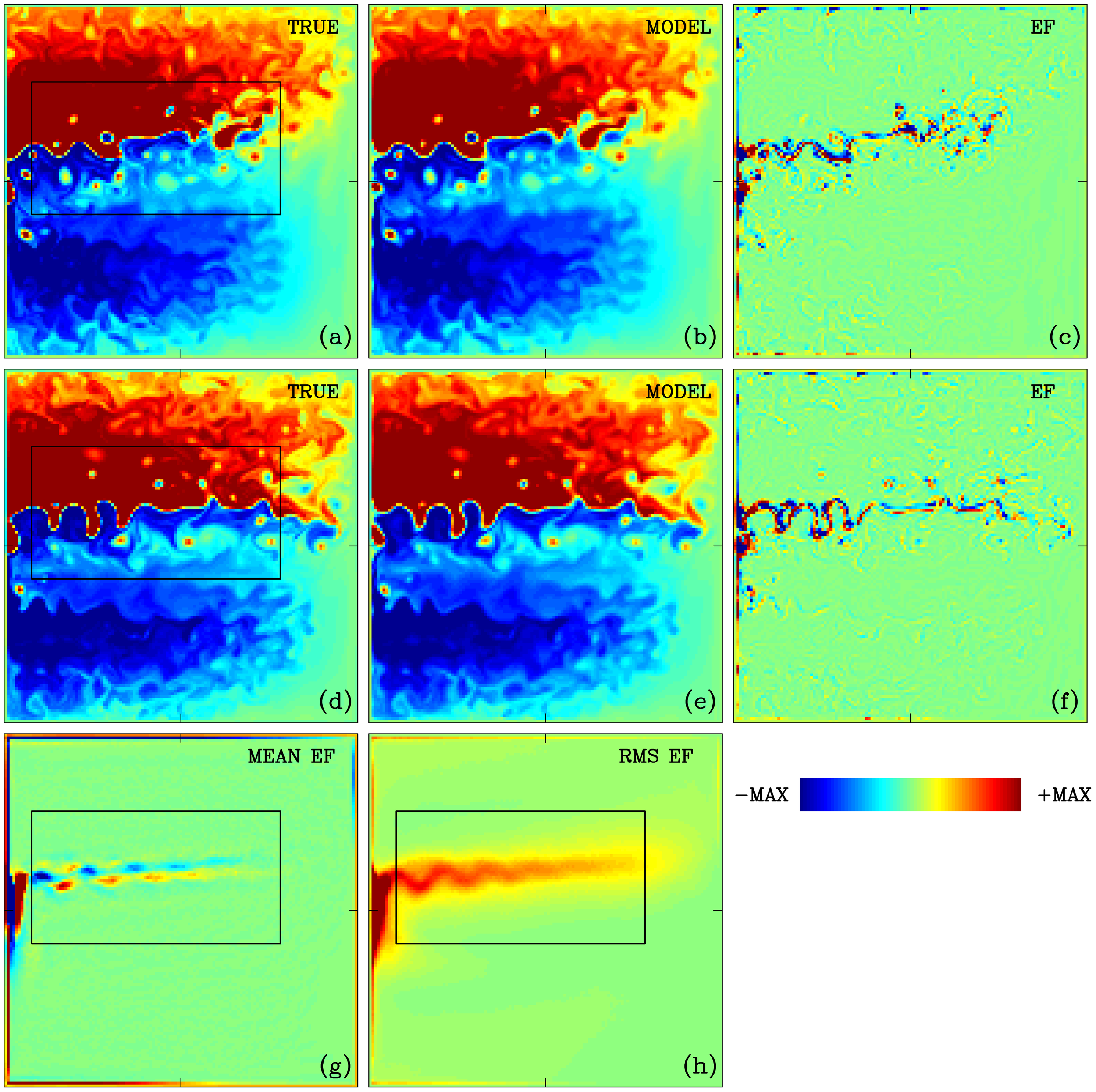
Figure 1. Reference eddy-resolving double-gyre model solution and its approximation. Note that the eastward jet possesses intense mesoscale variability, which in turn supports the jet. All panels show upper-ocean potential vorticity (PV) anomaly and its statistical moments, as plots on the coarse 129² grid. Top and middle rows of panels correspond to two different snapshots. (a, d) The reference eddy-resolving solution subsampled on the coarse grid. (b, e) The coarse-grid solution integrated over 4 days without any corrections, until the time shown in (a, d). (c, f) The difference between the reference and coarse-grid model solutions, which can be interpreted as the eddies. (g, h) The time-mean and standard deviation fields of the eddies, and color scale of the former is 10 times smaller, thus indicating that the time-mean eddies are relatively small. Units of the plotted fields are non-dimensional, with the length scale L = 30 × 10⁵ cm (the coarse-grid interval) and velocity scale U = 1.0 cm s⁻¹. These dimensions are consistently used across all figures in the paper. Colorbar MAX is equal to 150 (a, b, d, e), 50 (c, f, h), and 10 (g).

2.3 Eddy forcing

This section discusses eddy forcing, which represents eddy effects missing in the coarse-grid solution. The standard approach (Section 1.1) is to filter out the eddy component (denoted by primes) from the large-scale component (denoted by bars) and consider eddy forcing given by the

\begin{array}{l} \frac{\partial \bar{q_{1}}}{\partial t} + J (\bar{ψ_{1}}, \bar{q_{1}}) + β \frac{\partial \bar{ψ_{1}}}{\partial x} = W - F_{1} + ν \nabla^{4} \bar{ψ_{1}}, & (9) \end{array}

\begin{array}{l} F_{1} = \nabla \dot{(} u_{1}^{'} \bar{q_{1}} + \bar{u_{1}} q_{1}^{'} + u_{1}^{'} q_{1}^{'}) + \frac{\partial q_{1}^{'}}{\partial t} + β \frac{\partial ψ_{1}^{'}}{\partial x} - ν \nabla^{4} ψ_{1}^{'}, & (10) \end{array}

where only the upper-layer equation and eddy forcing $F_{1}$ are shown for brevity, and $u_{1} = (- \frac{\partial ψ_{1}}{\partial y}, \frac{\partial ψ_{1}}{\partial x})$ is the upper-layer flow velocity. Note that the other and more common approach for isolating the eddy forcing term is to filter the equations, but in this case, the filtering operation does not necessarily commute with the derivatives, and the lucidity of the dynamics is lost. Another important aspect is that Equations 9 and 10, which are cleanly formulated on the fine eddy-resolving grid, will be contaminated by unavoidable discretization errors when one rewrites them on the coarse grid of a non-eddy-resolving model. In this situation, the residual error can be absorbed into the eddy forcing term, but this implementation can be completely bypassed if we estimate eddy forcing directly by fitting the reference solution into the coarse-grid dynamics. In other words, we subsampled¹ the stream function of the reference solution on the coarse grid, obtained the corresponding PV field by differentiation, then treated this solution as the large-scale one, and substituted it (as barred fields) into Equation 9. We treated the resulting residual field as the eddy forcing (in all layers), which ideally corrects the coarse-grid model dynamics to reproduce the reference solution. The downside is that we do not have an explicit description of the eddies, but this is actually not a problem, as we only need an appropriate eddy forcing description.

To start illustrating the eddy forcing properties, let us explain how the differences between the reference and coarse-grid solutions are obtained. Figures 1b, e show coarse-grid model solutions corresponding to Figures 1a, d and started from the reference-state initial solution 4 days earlier—only very close visual inspection reveals the small differences that accumulated over this time. These differences, divided by the time interval, provide an approximation of the eddy forcing, shown in Figures 1c, f. We repeated this for 2-day and 1-day intervals and also looked at the eddy forcing calculated over the time step of the coarse-grid model. The shorter-time approximations of the eddy forcing become noisier, but their relations to the eastward jet and the corresponding spatial correlations (see below) remain qualitatively similar. We mostly considered the 2-day approximation and, for initial simplicity, focused on the upper-ocean eddy forcing and its parameterization because contributions from the deep-ocean eddy forcing turned out to be relatively small. As can be seen in Figures 1c, f–h, the eddy forcing is concentrated along the eastward jet and in the western-boundary currents, upstream of their confluence location. Eddy activity near the western boundary is dominated by strong and intermittent vortices emerging on the subtropical-gyre side (Figures 1a, d) and interpreted as intense transient meandering upstream of the confluence and eastward-jet separation point. Such behavior is more typical of the Kuroshio current rather than the Gulf Stream current (Hirata et al., 2025), and in real oceans, it may be controlled by the coastline and bottom topography, which are absent in our idealized double-gyre model.

For the sake of initial simplicity with the eddy parameterization, we opted to focus only on the eddy effects in the eastward jet region, which is indicated by a rectangle in Figure 1. Circulation in the remaining part of the ocean basin is either untouched by any parameterization or strongly (with a 10-day relaxation time scale) relaxed toward the reference time-mean state. The latter applies to each isopycnal layer in the seven most western rows of the grid points (a band of approximately 200 km wide near the western boundary). In fact, the main motivation to exclude the western-boundary region from the eddy parameterization is because it is dominated not by the eddy backscatter but by the viscous boundary layer region, which fluxes through the boundary different amounts of relative vorticity, when it is poorly resolved, thus leading to a different global PV balance of the gyres and overall much weaker PV contrast between them (e.g., Kurashina et al., 2021). Finally, by observing a small, relative to its variability, time-mean part of the eddy forcing (Figures 1g, h), we confirm earlier findings (Berloff, 2016) that the eddy backscatter is driven mostly by the transient eddy forcing, although the time-mean eddy forcing component is also correlated with the eastward jet in the sense of maintaining it.

It may seem that the eddy forcing can be parameterized as a simple space–time correlated process with the observed variance (e.g., Berloff, 2005; Ryzhov et al., 2019), but this does not work within the present framework and makes it an important point to discuss. Before we explain why this does not work in our case, let us point out that in the above-mentioned papers, the eddies are defined either as significant deviations from the reference field or by common spatio-temporal filtering. In either case, both the eddies and eddy forcing have large amplitudes and intensively hammer the corresponding coarse-grid solutions. On the contrary, in the present study, we define eddy forcing in a minimalistic way and simultaneously require that the augmented coarse-grid solution is objectively perfect (i.e., coincides with the reference one). The outcome remarkably combines the diagnostics of the gentle eddy forcing and the maximization of the role played by the coarse-grid dynamics.

First, we conducted several experiments in which the observed spatio-temporal history of the eddy forcing was imposed on the coarse-grid model dynamics, also initialized from the correct reference state. In such an experiment, a small round-up numerical error appears immediately and starts accumulating exponentially. After approximately 100 days, this error begins to have an impact and results in significant spatial decorrelation between the imposed eddy forcing and the actual large-scale, coarse-grid flow solution. Soon after, this decorrelation becomes critical, the eddy forcing rapidly loses its efficiency in maintaining the eastward jet, and the jet in the solution begins to fade away and gradually disappears. In effect, this completely wipes out any parameterization skills. If the round-up error is interactively corrected, then the correlations are never degraded, and the resulting solution is trivially perfect. From these experiments, we concluded that preserving correlations between any eddy forcing approximation of the parameterization closure and the coarse-grid modeled eastward jet is essential. To formalize these correlations, in the eastward jet subdomain, we closely looked at the eddy forcing evolving in time and monitored its relation to the corresponding PV anomaly, relative vorticity, and flow speed (Figure 2), all taken only in the upper ocean, for initial simplicity.

Figure 2

Four-panel data visualization: (a) PVA shows a red to blue gradient; (b) EF primarily in light green tones; (c) SPEED highlighted in red and yellow; (d) REL VORT with blue and green hues. A color bar ranges from blue (-MAX) to red (+MAX).

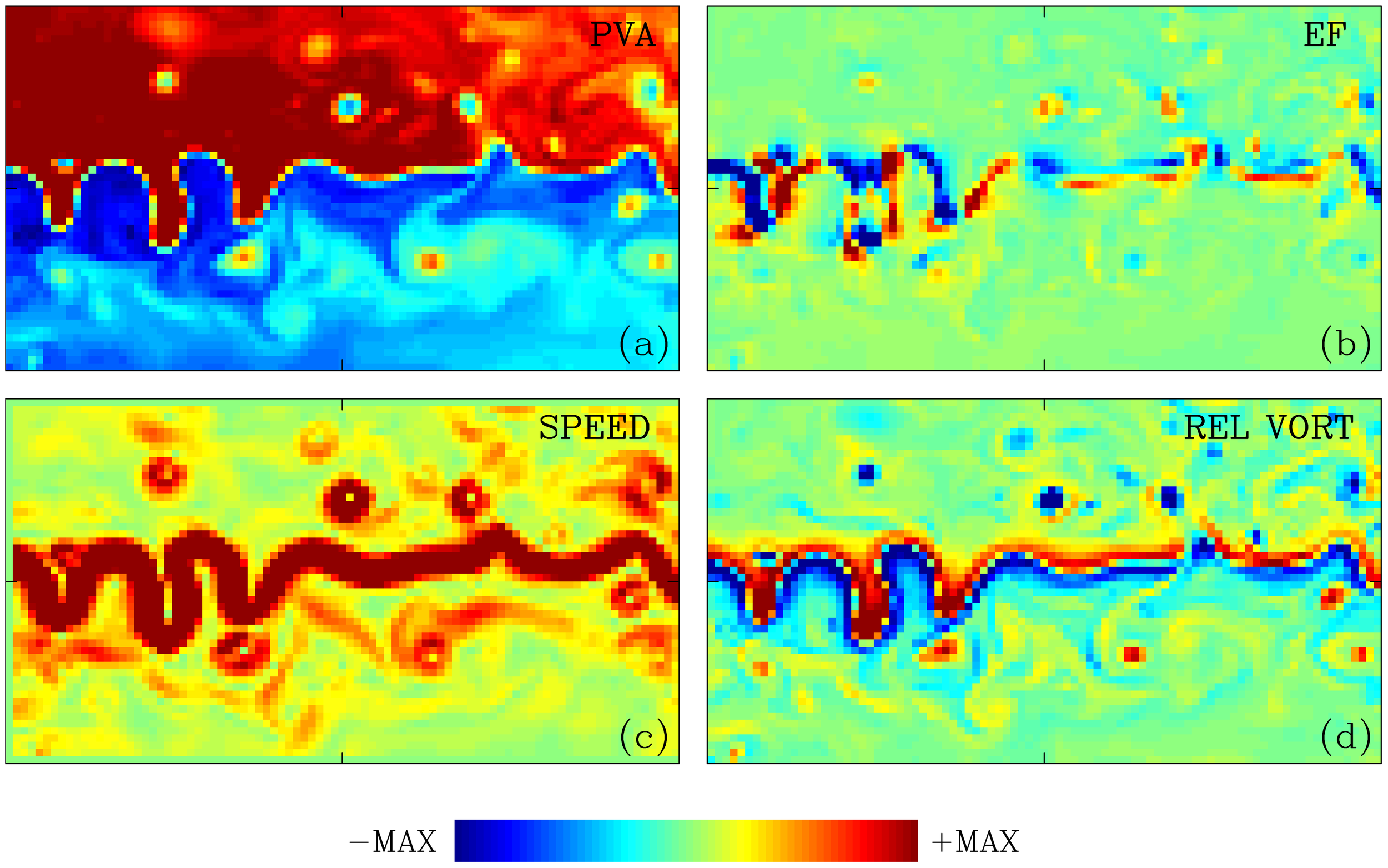
Figure 2. Snapshot of the eddy forcing in the eastward jet region. Upper-ocean fields are shown in the subregion (indicated in Figure 1 ) containing the eastward jet: (a) potential vorticity (PV) anomaly, (b) eddy forcing, (c) flow speed, and (d) relative vorticity. Colorbar MAX is equal to 180 (a), 20 (b), 0.4 m s⁻¹ (c), and 70 (d). Eddy forcing is systematically (anti)correlated with PV anomaly, with a correlation coefficient of approximately 0.5, and the corresponding correlation with the relative vorticity is approximately 0.6.

First, we restricted the consideration of correlations only to the fastest part of the instantaneous flow, with the speed exceeding $U_{c u t o f f} = 0.2$ m $s^{- 1}$ ; this is mostly a band straddling the eastward jet core and some detached vortex rings (Figure 2c). Clearly, the bulk of the eddy forcing amplitude is located within the fastest flows, where also the most significant errors appear due to the spatial coarse-gridding. Second, within the evolving fast-flow subdomain, we spatially correlated the eddy forcing with the selected PV and relative-vorticity fields. We found that the time-mean correlation with the relative vorticity is approximately 0.6, whereas with the PV anomaly, it is approximately 0.5. Both correlations are so large and significant that they can potentially serve as a basis for some eddy parameterization closure.

We checked and confirmed that the eddy forcing indeed injects energy into the coarse-grid large-scale flow in the eastward jet region. This is consistent with the popular eddy energy backscatter idea discussed in Section 1.1. We also translated the diagnosed eddy forcing into the local eddy diffusivity coefficient by dividing it locally by the PV Laplacian operator. This simple exercise produced highly inhomogeneous and complicated maps of the eddy diffusivity, with a weak negative average. From this, we concluded that the negative diffusion (i.e., up-gradient PV transport) idea is potentially applicable but should be implemented cautiously and most likely in some spatially averaged way in order to avoid noisy eddy forcing approximations and to preserve global correlations, first of all. Finally, we noted that because of the employed PV dynamics, which combines, connects, and constrains momentum and buoyancy effects, the eddy forcing injects both kinetic and potential energies. This observation suggests that both energy backscatters are to be considered and taken into account in the primitive-equation models, which do not impose exact PV balance. In the next section, we develop a simple parameterization and test its skills, all conducted within the PV dynamics framework, without resorting to the energetics and energy backscatters.

3 Closure implementation and testing

Given the discovery of the encouraging correlations between the eddy forcing and large-scale flow fields in the previous section, we focused only on the upper-ocean fields and calculated some important integral characteristics, all presented in Figure 3 and needed here for the data-driven construction of the parameterization closure. First, we considered separately both eddy forcing parts, which are located on the positive and negative sides of the relative-vorticity field. This gave us two separate, time-mean characteristics of the eddy forcing: $〈 F_{1}^{+} (x) 〉$ and $〈 F_{1}^{-} (x) 〉$ , where the functions with the plus/minus superscripts are individual, meridionally integrated and zonally varying eddy forcings, and the angled brackets indicate the time averaging, as elsewhere. The resulting characteristics (Figure 3a) show that the eddy forcing intensity tends to decay nearly monotonically, along the eastward jet, and in the eastward direction. Integrals under these curves are the key characteristics that we aim to represent and respect by the eddy parameterization closure. For easier understanding of the following technicalities, let us state upfront that the parameterization can be viewed as an extra forcing term appearing on the right-hand side of the dynamics and symbolically described as the following term (here, acting only in the upper layer, for simplicity):

Figure 3

Five line graphs display different analyses. Graph (a) shows “EF MEAN” against X [NONDIM], with values ranging from -40 to 30. Graph (b) illustrates “EF INT” versus time in years, ranging from -25 to 25. Graph (c) presents “PVA MEAN REL MEAN” against X [NONDIM], with values from -600 to 600. Graph (d) shows “PVA INT” over time, from -5 to 6. Graph (e) indicates “RATIO” plotted against X [NONDIM], with values from -40 to 30.

Figure 3. Integral characteristics of various upper-ocean properties in the eastward jet region. (a) Time mean (minus) eddy forcing in the vicinity of the eastward jet axis, plotted as a function of longitude; horizontal span on the plot corresponds to the eastward jet region; the upper and lower curves correspond to the northern and southern flanks of the jet, respectively. (b) Temporal variabilities of the integral values of the eddy forcing corresponding to the northern and southern flanks of the jet (values are scaled by 10⁻²). (c) The same as panel a, but for the potential vorticity (PV) anomaly (the corresponding external pair of curves is shown by thick lines) and relative vorticity (the corresponding internal pair of curves is shown by thin lines). (d) As in panel b, but for the PV anomaly contents. (e) Ratio of the eddy forcing curves from (a) to the curves in (c) Horizontal lines in (b, d) indicate the time-mean values, and in (e), they indicate the average ratios.

\begin{array}{l} \frac{D q}{D t} = \dots + C (t) M (t, x) q, & (11) \end{array}

where $q (t, x)$ is the evolving coarse-grid PV anomaly, $M (t, x)$ is the interactively estimated spatial mask that decides, where the extra forcing has to be applied, and $C (t)$ is the interactively estimated calibration coefficient that controls the strength of the extra forcing. Further below, we explain in detail how the mask and the calibration coeffcient in Equation (11) are found in the process of integrating the model.

Next, we calculated integrals of the corresponding time varying extensions, $F_{1}^{+} (t, x)$ and $F_{1}^{-} (t, x),$ denoted as $[F_{1}^{+}] (t)$ and $[F_{1}^{-}] (t)$ , respectively, and illustrated by Figure 3b. These integrals vary around their time-mean values rather modestly; therefore, as part of the parameterization closure, we opted to satisfy them only in the time-mean sense, at least for the initial simplicity. Jumping ahead, it is likely that this simplification resulted in excessive and under-constrained large-scale, low-frequency variability of the parameterized solutions, but we will get back to this further below. We found similar monotonic x-dependences in the time-mean integral characteristics for both PV anomaly and relative vorticity, as shown in Figure 3c. The corresponding time dependences for similarly calculated PV anomaly integrals, $Q_{1}^{+} (t, x)$ and $Q_{1}^{-} (t, x)$ are denoted as $[Q_{1}^{+}] (t)$ and $[Q_{1}^{-}] (t)$ , respectively. Figure 3d shows the relatively intense variability of these integrals, and for the relative vorticity, such variabilities are noticeably larger (not shown). Next, we considered ratios of the considered eddy forcing and circulation characteristics and plotted the outcome in Figure 3e. Clearly, the time-mean eddy forcing is roughly proportional to the time-mean PV anomaly content, and therefore, it can be potentially estimated from the PV anomaly distribution. It is not guaranteed that this will work because the circulation may drift out of this regime and become significantly different. Nevertheless, in the following part of the story, we have chosen to relate parameterized eddy forcing to the PV anomaly because, in comparison with the relative vorticity, it is a spatially smoother and temporally less varying field. Additional tests showed that the smoother the field used for the closure, the more robust the closure performance, thus providing motivation for the choice.

Before we illustrate the actual performance of our simple parameterization and closure, let us summarize its essentials and implementation. The coarse-grid model is initialized by an instantaneous snapshot from the reference solution and integrated in time, so at each time step, some extra forcing is added to the governing dynamics, but only in the eastward-jet subdomain and only in the upper ocean. In addition, the western-boundary region is fixed by strong relaxation, as explained in Section 2, because this region is deliberately kept outside the scope of the considered eddy effects and their parameterization. From the coarse-grid model, we diagnose the flow speed and restrict the interactive correction to the subdomain characterized by speed exceeding $U_{c u t o f f} = 0.2$ m $s^{- 1}$ , as explained in Section 2. In effect, this is the application of a spatial mask that constrains the action of the eddy parameterization to where its bulk should be, as suggested by the reference data analysis. The modest variation of parameter $U_{c u t o f f}$ is not essential, as we checked out. Next, we calculate the corresponding PV anomaly integrals, inside the mask and over each flank of the jet, and multiply the involved PV anomaly fields by a constant about unity so that the corresponding PV corrections, which are typically enhancing PV contrast across the jet, have area integrals equivalent to the eddy forcing integrals $〈 [F_{1}^{+}] 〉$ and $〈 [F_{1}^{-}] 〉$ . In other words, we enhance the PV contrast across the eastward jet with a constant rate based on the time-mean effect of the eddy forcing. All the involved information, with only one exception, is either provided interactively by the coarse-grid model solution or taken from the analyses of the reference “truth” and treated as the observed data.

The only key control parameter of the closure, referred to as the calibration parameter $C_{c}$ , needs special discussion, as well as interpretation and justification. As shown further below, the relevant underlying physics is simple and evident from comparing the reference and parameterized solutions. The reference eddy-resolving solutions have more substantial cross-jet, inter-gyre exchange of PV due to the more intensive formation of coherent vortices generated by growing meanders and eventually detached into the opposite gyre. These vortices transport material and PV into the opposite gyre and are partially resolved on the coarse grid, but their population and intensities become significantly diminished. Thus, they are not part of the eddy forcing; therefore, their effect is not parameterized and goes partially missing. The PV transport driven by this missing effect substantially cools down the cross-jet PV contrast between the gyres and, thus, counteracts the global effect of the eddy forcing backscatter. Instead of trying to compensate for this effect by a direct parameterization ², we opted to reduce the backscatter by deflating the approximation of the eddy forcing imposed by the parameterization. Our simple empirical choice of the corresponding calibration coefficient is $C_{c} = 0.25$ , and its initial tuning was qualitative, approximate, and based on the desire to keep the global energy level of the parameterized solution about right. We varied the calibration coefficient by approximately 20%, and these experiments showed that this variation in effect deamplifies or amplifies the eastward jet, and any further increase makes it unrealistically strong. With all the above aspects explained, we can now demonstrate the efficiency of the proposed parameterization.

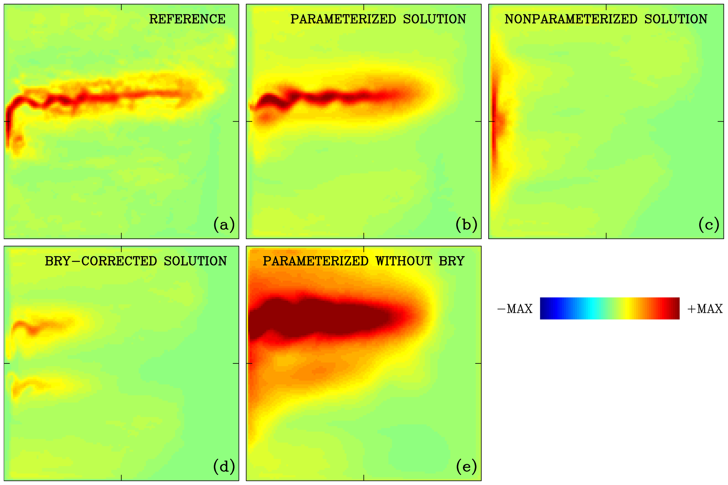
In Figures 4 and 5, we show instantaneous snapshots and time-mean fields of the reference, parameterized, and a few more solutions, all of which were spun up into statistically equilibrated flow regimes and saved over 100 years for further analyses. The comparison of the reference and parameterized solutions provides the upper bound for parameterization skills, as the former solution is the ideal target for the latter. The comparison of panels (a) and (b) in these figures illustrates that the parameterization has great skills in terms of restoring the eastward jet. Panel (c) shows a completely non-parameterized solution, which represents the lower bound for parameterization skills. This is what the raw coarse-grid model (i.e., without any corrections) predicts. Obviously, this solution does not reproduce the eastward jet at all, and, therefore, it is a complete failure. Two more solutions, which we show for comparison, strengthen our conclusions and interpretation. Panel (d) shows a non-parameterized solution with the western-boundary region corrected by the nudging explained in Section 2. Clearly, this solution has improved the ocean gyres by fixing the relative-vorticity flux through the western wall, which in turn is due to the improvement of the boundary layer velocity profile. Most importantly for the story, this solution has no eastward jet at all, thus proving our point that the jet is maintained mostly by the local eddy forcing via the backscatter mechanism.

Figure 4

Five panels display color-coded solutions ranging from blue to red, indicating increasing values. (a) Reference, (b) Parameterized Solution, (c) Nonparameterized Solution, (d) BRY-Corrected Solution, (e) Parameterized without BRY. A color bar at the bottom shows a gradient from blue (-MAX) to red (+MAX).

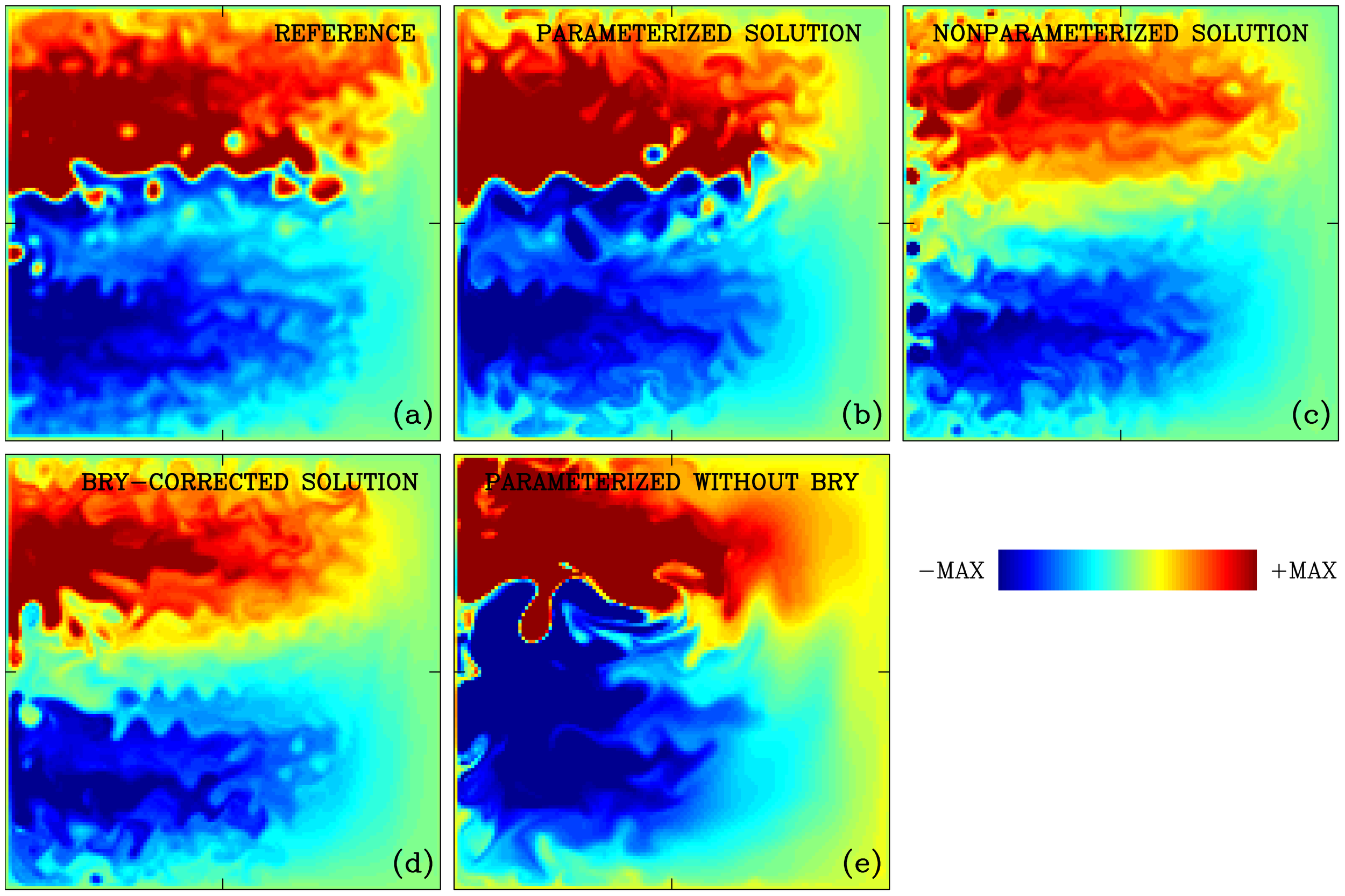
Figure 4. Typical upper-ocean potential vorticity (PV) anomaly snapshots of the key solutions. (a) Reference, (b) fully parameterized, (c) non-parameterized, (d) only boundary-corrected, and (e) only jet-parameterized solutions. The non-dimensional fields are plotted with the same color scale (MAX = 150).

Figure 5

Five panels show different fluid flow solutions with a color gradient from blue to red indicating values from negative maximum to positive maximum. Panel (a) is labeled “REFERENCE,” (b) “PARAMETERIZED SOLUTION,” (c) “NONPARAMETERIZED SOLUTION,” (d) “BRY-CORRECTED SOLUTION,” and (e) “PARAMETERIZED WITHOUT BRY.” Each panel exhibits variations in color distribution reflecting different solutions.

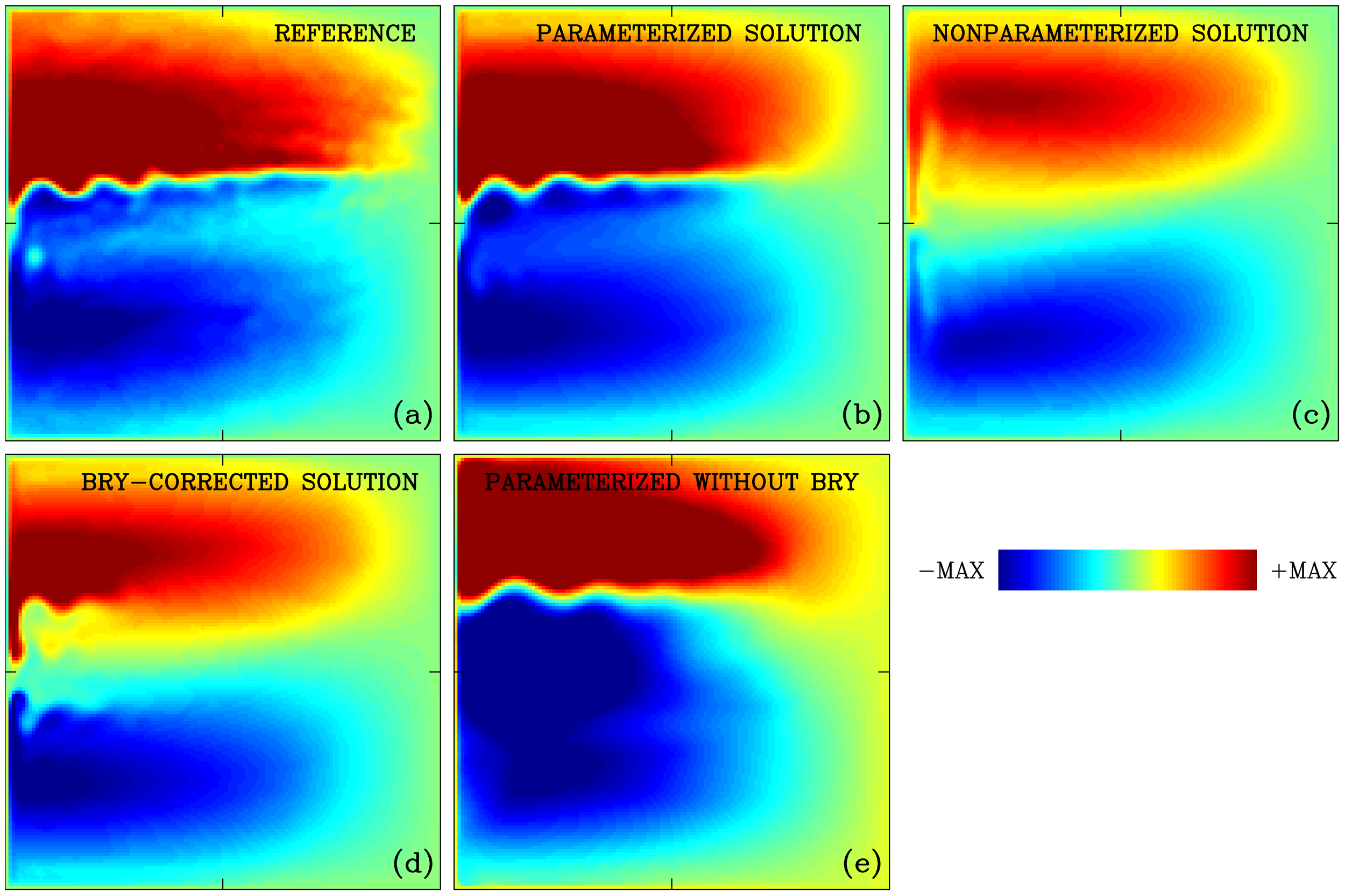
Figure 5. As in Figures 4, but for the time-mean fields. (a) Reference, (b) fully parameterized, (c) non-parameterized, (d) only boundary-corrected, and (e) only jet-parameterized solutions.

Finally, in panel (e), we show what happens with the flow if our parameterization closure is turned on, but the western-boundary region is not fixed. This experiment answers the legitimate question on the actual importance of the implemented western-boundary correction of the model. We found that both the inter-gyre PV contrast and the eastward jet become unrealistically strong, and in addition, viscous relative-vorticity flux through the western wall becomes completely unrealistic due to persistent and violent instabilities and eddies of the western-boundary currents. Clearly, fixing the eddy backscatter effect in the interior must be accompanied by the augmentation of the underresolution problem in the boundary—this statement is not trivial because fixing only one out of two problems makes things even worse. Here, our approach is to flag up the importance of the viscous boundary region parameterization, to defer its development for the future, and to focus on developing a closed parameterization only for the eddy backscatter.

For assessing errors of the explored solutions and quality of the parameterization, in addition to considering the time-mean circulation fields, we also considered second-order statistical moments. In Figure 6, we show the standard deviation of the upper-ocean PV anomaly in the demonstrated solutions: the parameterized solution looks much closer to the reference, but its variability is more intense and more smeared in space, as explained by somewhat overestimated large-scale low-frequency variability. Either the other solutions have no jet, hence no variability, or, on the opposite, there is an overestimated and misplaced jet in the last solution of the sequence. This solution is remarkably bad only because it attempts to parameterize the eddy backscatter without handling the western-boundary parameterization problem.

Figure 6

Five heatmaps comparing different solutions with a color scale ranging from blue (negative) to red (positive): 1. Reference (a): Yellow and red patterns showing complex details. 2. Parameterized Solution (b): Similar red patterns with clearer contours. 3. Nonparameterized Solution (c): Mostly green, few red areas. 4. BRY-Corrected Solution (d): Resembles the reference with notable red patterns. 5. Parameterized Without BRY (e): Dominantly red, less variation.

Figure 6. As in Figures 4, but for the standard deviation. (a) Reference, (b) fully parameterized, (c) non-parameterized, (d) only boundary-corrected solutions, and (e) jet-parameterized solution without boundary correction.

We characterized all the coarse-grid solutions formally by calculating the errors of the time-mean and standard deviation relative to the reference solution and showed these errors in pairs (E₁, E₂). Each error is estimated in the non-dimensional units and L₂-norm, as the average over the upper ocean, eastward-jet subdomain. The non-parameterized solution has error (41, 21.3), which can be viewed as the lower bound on performance, and only the last solution is worse, with the error (84.2, 58). From this lower bound, the implementation of the boundary correction reduces the error to (36, 21), which is a very small improvement, whereas the implementation of the parameterization closure massively reduces the error down to (16.1, 13.7). We treat this as a demonstration of the convincing success of the parameterization and also as the establishment of a solid starting position for any further improvements and developments.

Finally, we have to mention the temporal variability of the discussed solutions, and it is easily illuminated by the time series of globally averaged potential and kinetic energies (Figure 7). All solutions without the eastward jet demonstrate low levels of energies and weak variability, whereas the last solution, with the parameterization but without the boundary correction, predictably demonstrates the opposite behavior. The most important comparison is between the reference and parameterized solutions, and it demonstrates the excessive variability of potential energy in the latter. This is the most evident shortcoming of our simple parameterization, and it basically describes the decadal anomalous elongations and contractions of the eastward jet and its recirculation zones, as clearly seen from the animations of the circulation (not shown). We defer fixing this problem to the future, and we hypothesize that it appears from the fact that we keep the calibration coefficient C_c constant for all the states and phases of the eastward jet, whereas it can be made variable in accord with the data. At this point, our parameterization story came to an end, and we are ready to summarize what has been achieved and to provide a critical discussion in the next section.

Figure 7

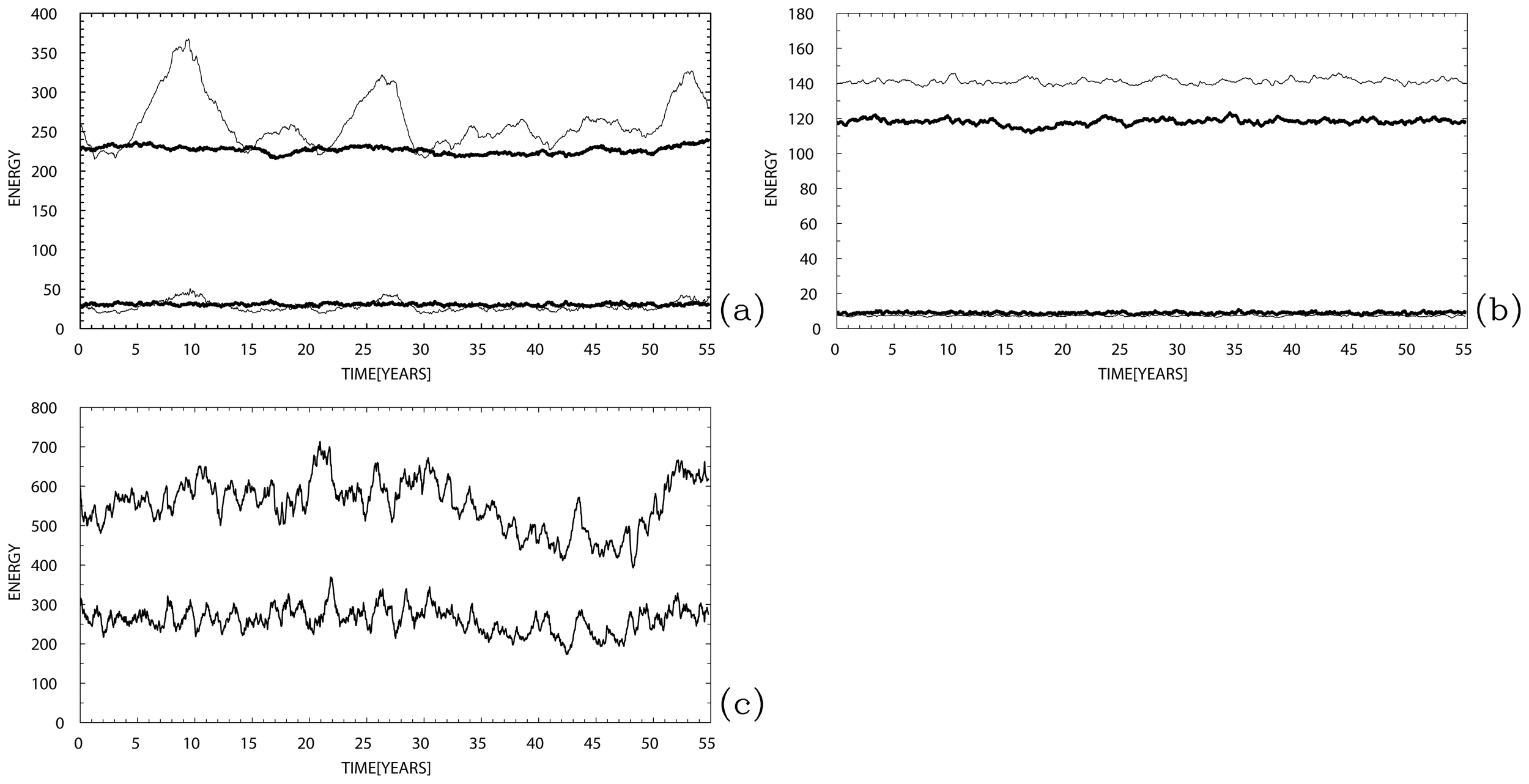
Three line graphs labeled (a), (b), and (c) depict energy variation over time in years. Graph (a) shows three series with energy spikes. Graph (b) indicates stable energy levels, while graph (c) displays two series with fluctuating patterns.

Figure 7. Total potential (upper) and kinetic (lower curve) energy time series. (a) Energies of the reference (thick) and fully parameterized (thin curves) solutions; mostly in the upper layer, the parameterized solution exhibits excessive low-frequency variability corresponding to overestimated phases of the eastward jet strengthening and weakening. (b) Energies of the non-parameterized (thick) and only boundary-corrected (thin curves) solutions; note that both solutions have significantly low energies, and the boundary correction has small impact on the energy level. (c) Potential (upper) and kinetic (lower curve) energies of the solution with parameterized jet but without fixed western-boundary layer; note that the energies are significantly overestimated and exhibit excessive variability, and the kinetic energy becomes similar in amplitude to the potential one. Note that the vertical-axis interval is different across the panels, the values are non-dimensional, and each energy is integrated over the basin and divided by the basin area (i.e., basin-averaged).

4 Summary and discussion

Mesoscale eddies, which can be viewed as “weather” of the ocean, play many important roles in the oceanic large-scale general circulation and, most importantly, shape it through various effects and feedbacks. The importance of the eddy effects motivates researchers either to resolve them dynamically, via brute-force high-resolution computations of the OGCMs, or to represent them as eddy parameterizations. In the latter case, any parameterization must be eventually closed on the resolved circulation fields, which is a specific embodiment of the general turbulence closure problem. Thus, active research toward developing accurate, physically justified, and practically feasible eddy closures is already ongoing, at least over the last decades, and it shows no signs of ending.

In this paper, we considered a test case, an idealized eddy parameterization problem formulated within the classical, intermediate-complexity ocean dynamics paradigm of the wind-driven midlatitude gyres, which includes western-boundary currents and their eastward jet extension with the adjacent recirculation zones. First, this set-up nicely connects to the numerous existing literature on the subject (see Section 1). Second, it focuses on one of the most difficult to parameterize, the global-ocean eddying phenomenon, which significantly raises the value of the outcome. The implemented approach is perfectly testable, as it starts from some reference eddying (turbulent) solution, then it goes to extracting and analyzing the important eddy effects, and, finally, it develops and solves a non-eddy-resolving version of the ocean circulation model, armed with some built-in eddy closure and fully capable of reproducing the main features of the reference solution. It is shown with various metrics that the closure works well, in the sense that it provides significant and easily observed improvement of the model solution: the eastward jet is restored to a rather realistic level, as objectively judged by comparison with the reference solution, whereas without the closure, this jet is completely absent from the coarse-grid model. This success suggests that the closure indeed takes into account some most important aspects of the eddy effects, although one may argue that we picked up the most pronounced eddy-driven flow feature and focused on it and its recovery in the parameterized dynamics. Of course, no closure is perfect; therefore, some shortcomings of the parameterized solutions are pointed out and discussed, and the main of them is the excessive decadal variability of the eastward jet strength. Previous studies by Ryzhov et al. (2020) highlighted difficulties with reproducing the involved large-scale, low-frequency variability; therefore, finding such a deficiency in the proposed parameterization is not surprising. Most likely, some additional constraints have to be implemented to mitigate this problem.

Our study has several novelties, which are worth listing altogether. First, we do not define the eddies and deal only with the eddy forcing; thus, we avoid any ambiguity in defining the eddies, as this definition is a big problem by itself. Second, we defined the eddy forcing history in terms of the coarse-grid model spatio-temporal error field, arising when the model attempts to reproduce the reference data. This definition allows us to avoid any ambiguity in filtering out the eddy forcing. Third, we uncovered significant correlations between the eddy forcing and the eastward jet, and we argued that their effect, which mostly increases PV contrast across the jet, is a fundamentally important aspect for any parameterization of the eddy backscatter maintaining the jet. Fourth, our parameterization is data-driven, as we tuned it by extracting and utilizing some key information from observations, which in our case were supplied by the reference eddy-resolving solution. Fifth, for assessing skills of the eddy closure, we consider spatial patterns of the time-mean circulation and its variance, rather than isotropic power spectra of some fluctuations (i.e., eddy energy). This is because we are, first of all, interested in the restoration of the highly anisotropic eastward jet, rather than in maintaining some global eddy energy levels, which are an easier target. In effect, this approach significantly raises the standard for the required parameterization and closure skills. Sixth, we deliberately left out parameterization of the western-boundary region, which plays an important role in the global PV budget of the gyres but is also significantly misrepresented on the coarse grid. This process is not an eddy backscatter and should be parameterized separately, and we fixed it by simple nudging toward the flow climatology. We showed directly that neglecting the boundary-layer parameterization in combination with the implementation of the eddy backscatter parameterization produces the worst result. This elevates the importance of the western-boundary parameterization to the highest level, but we deliberately left this issue out of the paper’s scope.

The parameterization and its closure are organized so that the coarse-grid model is augmented only in the eastward jet region, and only in the upper ocean, and in the fast currents. This augmentation is implemented as an enhancement of the PV anomalies straddling the eastward jet, with the spatial integrals of the positive and negative augmentations being equal to the corresponding time-mean integrals of the observed eddy forcing. The actual eddy forcing is noisier than its implementation, and effectively, we redistributed its cumulative action in terms of modifying a much smoother PV field. The coarse-grid modeled eastward jet has reduced small-scale variability driving cross-jet PV fluxes, which counteract the eddy backscatter; therefore, we calibrated down the parameterized eddy effect by empirically reducing its strength. This calibration is the only important parameter that controls the closure.

Future extensions of the reported results should include a similar development of an eddy parameterization for the primitive-equation double-gyre model. In this case, some benchmark eddy-resolving solutions should also be used as the starting point, but the eddy effects are to be augmented separately into the momentum and buoyancy equations. Constraining these effects and balancing them with each other is an open question. The other useful and interesting development is obtaining various eddy forcing fields by the proposed method of feeding eddy-resolving reference solutions into some coarse-grid ocean models of interest. Finding significant correlations between various eddy forcings and some large-scale flow characteristics may result in discovering useful closures for the eddy parameterizations. On the next level of the eddy parameterization development, we envision the implementation of a more sophisticated closure based, most likely, on machine learning methods that will respect the key eddy–large-scale correlations in a more detailed way. Finally, our results suggest testing existing eddy parameterization ideas in flow regimes with a fully developed and coherent eastward jet extension.

Let us finish the story by elaborating on the broader applicability of the proposed closure and by making a few subjective general comments. First, we demonstrated that eddy effects can be unambiguously extracted in the process of training some coarse-grid models to represent given reference fields. This is a very general result that can be broadly adopted for training low-resolution models with high-resolution reference solutions. Second, we considered the notoriously difficult problem of eddy parameterization for midlatitude eastward jets and made significant progress; however, our success does not provide a final recipe for comprehensive GCMs and, instead, calls for the next study extending into primitive-equation frameworks. Whether such an extension will be successful is hard to predict; thus, our progress may be limited. The main problem, in our opinion, may be due to the necessity to account for mutual correlations between individual eddy forcings in the components of the momentum equation and thermodynamic equations. So far, the QG framework has provided a natural connection of all these eddy forcings into the unified potential vorticity description. Handling such correlations in addition to handling correlations with large-scale properties may be difficult. Third, we highlighted that the parameterization of the missing near-boundary physics is likely to be very different from the interior-basin eddy backscatter, and we provided no ideas for the parameterization of the former.

Data availability statement

The raw data supporting the conclusions of this article will be made available by the authors, without undue reservation.

Author contributions

PB: Data curation, Methodology, Visualization, Software, Conceptualization, Investigation, Writing – review & editing, Validation, Writing – original draft, Formal analysis. IS: Methodology, Data curation, Investigation, Writing – review & editing.

Funding

The author(s) declare that financial support was received for the research and/or publication of this article. Pavel Berloff was supported by the Moscow Center of Fundamental and Applied Mathematics at INM RAS (Agreement with the Ministry of Education and Science of the Russian Federation: 075-15-2025-347). Igor Shevchenko thanks the Natural Environment Research Council for the support of this work through the project AtlantiS (P11742).

Acknowledgments

Pavel Berloff, with deepest gratitude, acknowledges continuous support and advice from Bill Dewar on the series of research publications dealing with parameterizations for oceanic mesoscale eddies, and at present, this work is the last one in this sequence. The authors are grateful to the reviewers for their criticisms and suggestions.

Conflict of interest

The authors declare that the research was conducted in the absence of any commercial or financial relationships that could be construed as a potential conflict of interest.

The author(s) declared that they were an editorial board member of Frontiers, at the time of submission. This had no impact on the peer review process and the final decision.

Generative AI statement

The author(s) declare that no Generative AI was used in the creation of this manuscript.

Publisher’s note

All claims expressed in this article are solely those of the authors and do not necessarily represent those of their affiliated organizations, or those of the publisher, the editors and the reviewers. Any product that may be evaluated in this article, or claim that may be made by its manufacturer, is not guaranteed or endorsed by the publisher.

Footnotes

^ In principle, we could also use local averages over the fine-grid nodes contained within the coarse-grid cells. As shown by Berloff et al. (2021), such small modifications of the reference flow have small effects on the outcome, and we confirmed this in the present study.
^ We speculate that in the coarse-grid model, such vortices can be induced by highly localized forcing impacts, but developing this idea goes beyond the scope of this paper.

References

Agarwal N., Ryzhov E., Kondrashov D., and Berloff P. (2021). Correlation-based flow decomposition and statistical analysis of the eddy forcing. J. Fluid Mech. 924, A5. doi: 10.1017/jfm.2021.604