Abstract
Introduction:
The blue economy has become a pivotal framework for achieving sustainable development, emphasizing the responsible utilization of marine and coastal resources while preserving ecosystem integrity. Although biodiversity is central to fisheries, aquaculture, and coastal tourism, its direct role in shaping the blue economy remains underexplored. Furthermore, the interactions of biodiversity with other structural factors, such as financial development, institutional quality, and environmental pressures, are insufficiently addressed in existing studies.
Methods:
This study investigates the determinants of the blue economy by employing panel data from the world’s ten highest-income blue economies over the period 2000–2021. To address econometric challenges such as cross-sectional dependence, unit roots, and cointegration, second-generation panel techniques were applied. Long-term relationships were estimated using the Augmented Mean Group (AMG) estimator, and robustness was assessed through complementary econometric tests.
Results:
The empirical findings demonstrate that biodiversity exerts a positive and statistically significant effect on the blue economy. In contrast, financial development is negatively associated with blue economy performance. Institutional quality and per capita income are found to enhance blue economy outcomes, while CO₂ emissions exert a detrimental influence. Robustness checks confirm the stability and reliability of these results across alternative specifications.
Discussion:
The results underscore the vital role of biodiversity conservation in fostering sustainable growth within the blue economy framework. However, the negative effect of financial development suggests that existing financial structures do not sufficiently channel resources into environmentally sustainable marine activities. Strengthening institutional frameworks and aligning financial systems with ecological priorities are therefore critical. Moreover, reducing carbon emissions is indispensable to securing long-term resilience of marine ecosystems and ensuring the sustainability of blue economy activities.
Introduction
Covering 70% of the globe, seas and oceans are an important indicator of their significance for the welfare and peace of humanity. Seas and oceans offer important opportunities for the continuity of humanity, such as energy, safe food, and tourism. In this context, as emphasized in Sustainable Development Goal (SDG) 14, which focuses on life under water, marine ecosystems are vital for both biodiversity and economic activities. This situation has caused many researchers to conduct research in this field (Sarwar, 2022; Yasser et al., 2024).
One of the important concepts that these researchers focused on was the “blue economy”. The blue economy was formally introduced during the 2012 Rio+20 UN Sustainable Development Conference and encompasses the sustainable use of ocean resources, marine pollution management, and climate change impacts. The World Bank (2017) defines the blue economy as the sustainable use of ocean resources for economic growth, improved livelihoods, and maintaining ocean health. Similarly, the Organisation for Economic Co-operation and Development (OECD) (2016) views the blue economy as encompassing all economic activities related to the oceans, while the United Nations (2017) emphasizes the importance of sustainability in these efforts, aligning them with the broader goals of the SDGs (Keen et al., 2018; Benzaken and Hoareau, 2021). Discussions about the blue economy also include ocean privatization, governance, sustainability, equity, and the role of various actors (Bennett, 2018).
In parallel with the definition of the blue economy, the development of measurable indicators to monitor and evaluate the performance of the blue economy has been discussed. In this context, production-based and value-added indicators have come to the fore in the literature. These indicators include total fish production (TFP), aquaculture production (AFP), value added for the agriculture, forestry, and fishing sector (FGDP) (Alharthi and Hanif, 2020; Hossain et al., 2024; Ahammed et al., 2025). These indicators represent both the economic output of the blue economy and provide information on the sustainability and resilience of the marine ecosystem. For example, while TFP is an important component of the blue economy for food security and biodiversity conservation, AFP offers an alternative to traditional fishing practices. Similarly, FGDP serves as a broader economic indicator to assess the contribution of natural resource-based sectors, including marine activities, to national economies.
The effective development and sustainability of the blue economy are closely linked to a range of ecological, economic, and institutional factors. Among these, biodiversity plays a central role in maintaining the resilience and productivity of marine ecosystems, which directly support fisheries, aquaculture, and coastal tourism. A rich and balanced marine biodiversity is essential for the long-term sustainability of the natural resources on which the blue economy depends (Pimentel et al., 1997). Equally important, financial development facilitates investment in sustainable marine infrastructure, fisheries technology, and environmental protection initiatives, enabling economies to better capitalize on marine resources while preserving ecological balance (Nham and Ha, 2023). In addition, institutional quality determines the effectiveness of marine governance, environmental regulation, and the enforcement of sustainable practices, which are critical for managing shared ocean resources and mitigating risks associated with overexploitation and pollution (Hossain et al., 2024). On the other hand, CO2 emissions represent a major environmental pressure on marine ecosystems, contributing to ocean acidification, rising temperatures, and biodiversity loss, all of which can undermine the productivity and sustainability of blue economy sectors. Finally, GDP per capita reflects the broader economic development level of a country, influencing both the demand for marine-based goods and services and the capacity to invest in sustainable resource management (Petrea et al., 2021). Examining the dynamic relationships among these factors within the blue economy framework offers valuable insights for promoting inclusive, resilient, and environmentally sustainable growth in alignment with the objectives of SDG 14.
This study investigates the relationship between the blue economy, financial development, and biodiversity using second-generation unit root and cointegration tests, the Augmented Mean Group (AMG) estimator, and the Method of Moments Quantile Regression (MMQREG). Also, carbon emissions, institutional quality, and GDP per capita (GDPPER) are control variables in the study. The study makes several contributions to the literature. It is among the few studies that simultaneously examine the link between financial development, the blue economy, and biodiversity. Total fish production, agriculture, forestry, and fishing value-added, and aquaculture production are used to represent the blue economy, offering comprehensive insights into the factors affecting it. The inclusion of these variables also serves as a robustness check.
This research fills a significant gap in the literature by highlighting the underexplored nexus between financial activities and the blue economy, particularly blue finance’s role in sectors like fishing, coastal infrastructure, and marine conservation. Moreover, this study pioneers the exploration of the relationship between biodiversity and the blue economy, providing valuable insights for future research.
Theoretical and practical studies on the blue economy have examined its opportunities and challenges (Lee et al., 2020; Benzaken et al., 2024), but this empirical study contributes by offering policy-relevant findings. It incorporates institutional quality, GDP per capita, and CO2 emissions as control variables, providing nuanced insights into the determinants of the blue economy. This is the first study to use the second-generation unit root and cointegration tests, AMG estimator for benchmark, and MMQREG for sensitivity estimations, to analyze the relationship between the blue economy and financial development, offering a comprehensive evaluation of these relationships.
Literature review
The blue economy encompasses various sectors, including marine aquaculture, fishing, tourism, transportation, logistics, and oil and gas mining, all of which play a crucial role in global economic development and climate sustainability. Globally, the blue economy supports approximately 31 million jobs (Nham and Ha, 2023). Therefore, understanding the determinants of the blue economy is essential for informing policy decisions. This section reviews the relevant literature on the blue economy, focusing on its links to financial development and biodiversity.
Blue economy and biodiversity
Biodiversity encompasses the variety of plant and animal species at local, regional, and global scales, classified as genetic, species, and ecosystem diversity. Biodiversity provides essential environmental services, including carbon sequestration, oxygen production, soil protection, and water cycle maintenance. However, the loss of biodiversity exacerbates climate change and leads to rising sea levels, droughts, and floods.
Biodiversity is fundamental to food production, as it supports the variety of animals and plants essential for agriculture (Pimentel et al., 1997). Low levels of biodiversity are linked to increased disease transmission and higher healthcare costs (Keesing et al., 2010; Wilkinson et al., 2018). Additionally, biodiversity is critical for drug discovery (Neergheen-Bhujun et al., 2017). The global economy, particularly sectors like forestry, fisheries, and agriculture, depends heavily on ecosystem biodiversity, contributing trillions of dollars annually (World Economic Forum, 2020; World Bank, 2024). Biodiversity also offers natural protection from floods, storms, and soil erosion, while supporting water purification and waste management (World Economic Forum, 2020). Ensuring the sustainability of biodiversity presents an opportunity to reduce reliance on nonrenewable resources, enhance food security, mitigate climate change, and stimulate rural employment and economic growth (Turlakova, 2021). In this context, the following hypothesis will be followed in the study;
(H1): Biodiversity has a positive impact on the blue economy.
Blue economy and financial development
SDG14 focuses on the protection and sustainable use of oceans, seas, and marine resources. There is a broad consensus in the literature on blue economy finance that addressing the financing gap for sustainable development, especially in lower-income countries, is critical (Benzaken et al., 2024). The blue economy requires sufficient and affordable financial resources, and blue finance aims to address the current lack of standards, frameworks, financial incentives, and globally consistent methodologies (Narula et al., 2023). Financial resources supporting social, economic, and environmental sustainability are categorized under the umbrella of blue finance.
Blue finance focuses on programs designed to reduce pollution, mitigate CO2 emissions, implement sustainable regulations for marine resources, protect coastal environments, and improve energy efficiency. Key organizations like the Asian Development Bank, World Bank, United Nations Environment Programme, and European Union support blue economy projects. The term “Ocean Financing Facility” refers to accelerated investment initiatives targeting blue economy projects (Tirumala and Tiwari, 2022).
Research by Shiiba et al. (2022) highlights global and regional financing initiatives for marine conservation, while Evoh (2009) emphasizes the positive impact of digital financial transactions, such as those provided via mobile phones, on fishermen. Mallin et al. (2019) and Pascal et al. (2021) underscore the importance of public funds in managing maritime activities and maintaining marine protected zones. Green bonds, climate bonds, and blue bonds are identified as significant blue finance resources (Pascal et al., 2021). Conservation Trust Funds (CTFs) are financial tools designed to protect biodiversity and support projects related to ecosystem restoration, ecotourism, and sustainable fishing (Morgan et al., 2022). Nham and Ha (2023) found that financial development contributes to the sustainability of the blue economy, while Shan et al. (2023) highlighted the positive relationship between blue finance, digitalization, and sustainable credit. In this context, the following hypothesis will be followed in the study;
(H2): Financial development negatively affects the blue economy.
Additionally, the following hypotheses will be followed for control variables in this study;
Effective governance and regulations are critical for sustainable marine resource management. The results support this, showing that institutional quality enhances TFP, AFP, and FGDP.
(H3): Strong institutional quality positively influences the blue economy.
Emissions contribute to ocean acidification and biodiversity loss, harming marine ecosystems. The study finds consistent negative effects of CO2 emissions across all models.
(H4): CO2 emissions negatively impact the blue economy.
Economic growth enables investment in sustainable practices. The results show a positive relationship.
Hypothesis 5 (H5): Higher GDP per capita positively affects the blue economy.
Literature gap
The reviewed literature highlights the importance of both financial development and biodiversity in fostering the blue economy, but significant gaps remain. First, limited studies examining the nexus between financial activities and the blue economy. This study addresses this gap by exploring the affiliation between financial development and the blue economy, particularly focusing on fishing, coastal infrastructure, and marine conservation. Moreover, previous research has scarcely explored the link between biodiversity and the blue economy, which this study aims to investigate in depth. Additionally, while the role of blue finance has been acknowledged, the specific financial challenges faced by small and medium-sized enterprises in ocean-based sectors remain underexplored. This study seeks to contribute by examining how financial development influences the growth and innovation of blue economy sectors, including renewable energy, marine mining, and shipping. Addressing these research gaps, this study provides a foundation for future empirical investigations and contributes valuable insights to the existing literature on the blue economy, financial development, and biodiversity.
Data and methodology
Data
This study analyzes the influence of biodiversity on the blue economy for the 10 economies with the highest income from the seas and oceans in the 2000–2021 period. In this study, three variables (TFP, AFP, and FGDP) were selected to represent the blue economy following Alharthi and Hanif (2020), Hossain et al. (2024), Ahammed et al. (2025). According to Hossain et al. (2024), fishing and mariculture enhance coastal livelihoods, create jobs, and sustain ocean ecosystems by preserving fish stocks. This study uses total fisheries and aquaculture production in metric tons as dependent variables. Figures 1–3 present blue economy indicators. It is seen that China ranks first in the blue economy.
Figure 1
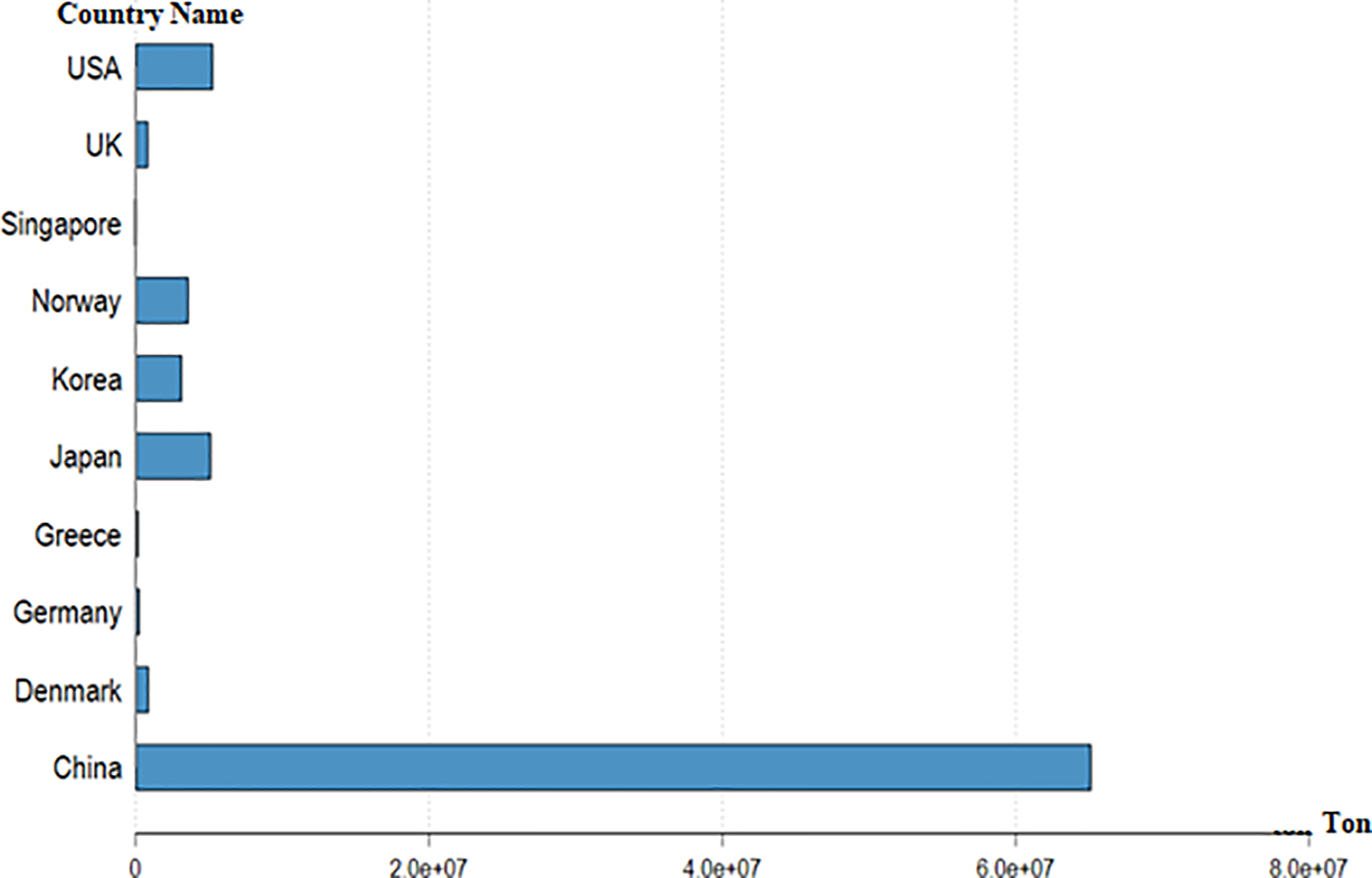
Mean of TFP.
Figure 2
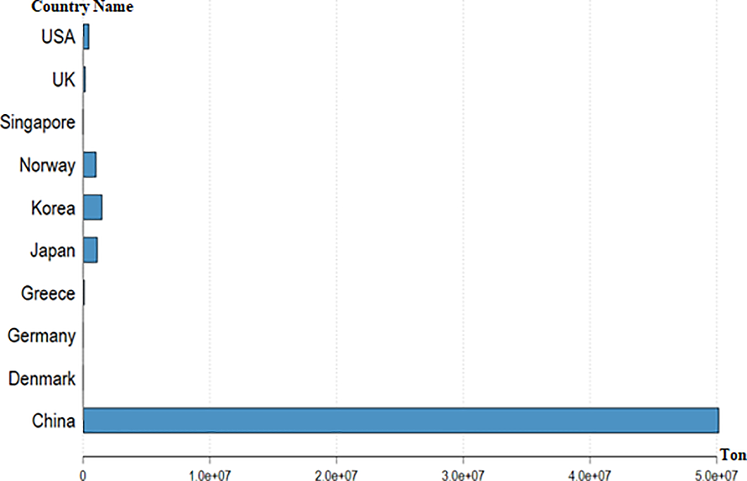
Mean of AFP.
Figure 3
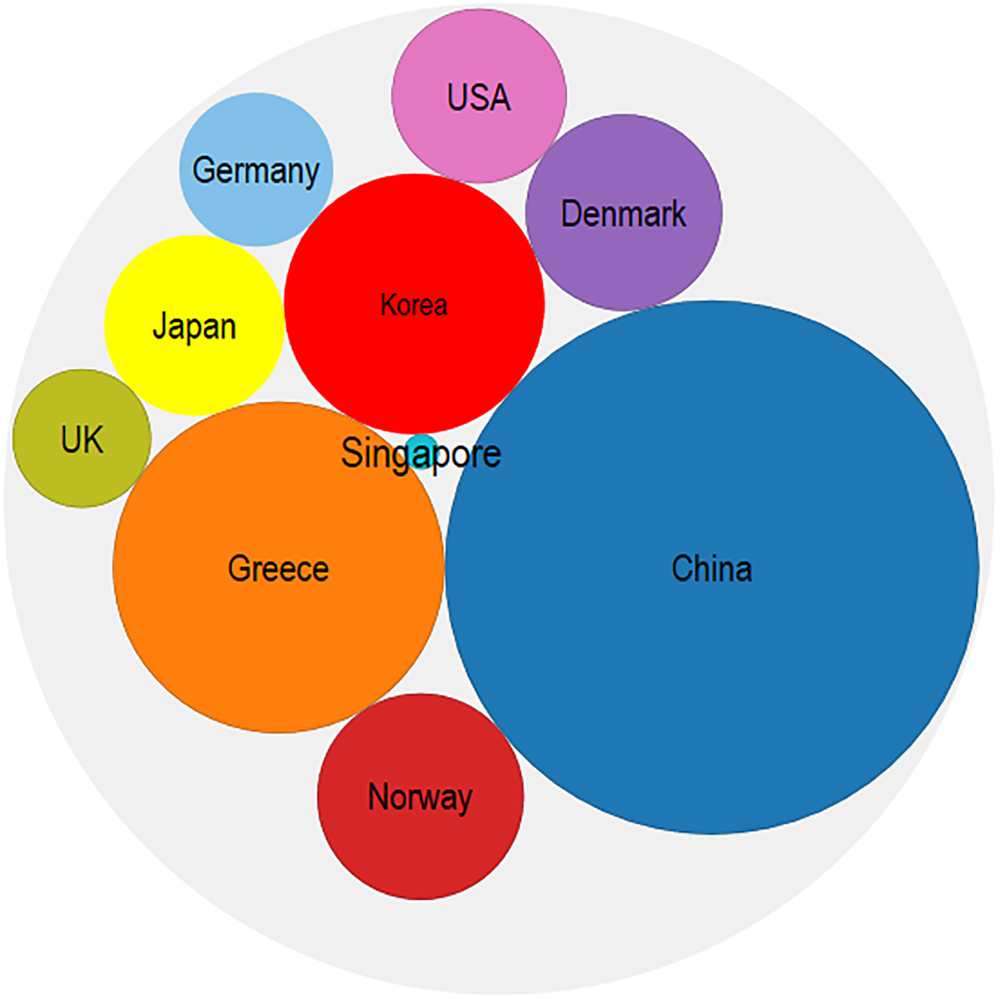
Mean of FGDP.
Figure 1 compares the TFP averages of the countries. According to the graphical results, China stands out as the country with the highest total production volume by far. Following China, the USA, Norway, and Japan are ranked with relatively lower rates, while the production amounts of other countries remain quite limited. This situation shows China’s dominant and decisive role in global fisheries production.
Figure 2 presents the AFP averages of the countries. The results reveal that China is also the absolute leader in aquaculture. While Japan, Norway, and the USA are the countries that follow it, the production levels of these countries are far behind China. The graphic shows that China has a very large production capacity not only in traditional fisheries but also in aquaculture activities worldwide.
Figure 3 compares the contributions of the countries’ fisheries sectors to gross domestic product (FGDP). China also stands out as the country with the highest value in this indicator. Greece, Korea, and Singapore stand out as the countries that follow China. The bubble chart structure visually and effectively presented the economic contribution of countries to the sector and once again demonstrated China’s superiority in this field.
The main independent variable of the study is biodiversity. Biodiversity plays an important role in various economic sectors such as agriculture, forestry, fisheries, and tourism. In agriculture, biodiversity contributes to sustainable food production by enhancing natural pest control, soil fertility, and crop pollination. Similarly, biodiversity-rich forests provide valuable resources such as timber and nontimber forest products, as well as essential ecosystem services such as carbon management and water regulation (Scheper et al., 2023). The Red List Index (RLI), published by the OECD and compiled by the International Union for Conservation of Nature (IUCN), was used as the biodiversity indicator (BIOD). The RLI is a metric that reflects trends in the overall extinction risk for groups of species across the globe. It specifically tracks the conservation status of species and is a key indicator for monitoring progress toward SDG15.5. The index is scaled between 0 and 1, where a value closer to 0 indicates a high risk of extinction for the assessed species, and a value approaching 1 reflects a lower risk and healthier biodiversity conditions. Figure 4 shows the biodiversity status of the countries. The rationale for selecting this index lies in its comprehensive, internationally standardized, and policy-relevant structure. Unlike broader measures of biodiversity that rely on habitat coverage or species richness alone, the RLI specifically tracks changes in the extinction risk of species over time, directly reflecting progress toward SDG15.5. Its bounded scale between 0 and 1 allows for clear cross-country comparability and temporal monitoring. A value closer to zero indicates a higher risk of extinction, while values approaching one reflect healthier biodiversity conditions. By focusing on species survival status, the red index provides a more actionable and ecologically meaningful measure, especially relevant for countries’ environmental sustainability agendas. According to this, Germany and Denmark are in a good situation in terms of biodiversity, while China and Korea are in a bad situation. Information on all variables in the study is presented in Table 1.
Figure 4
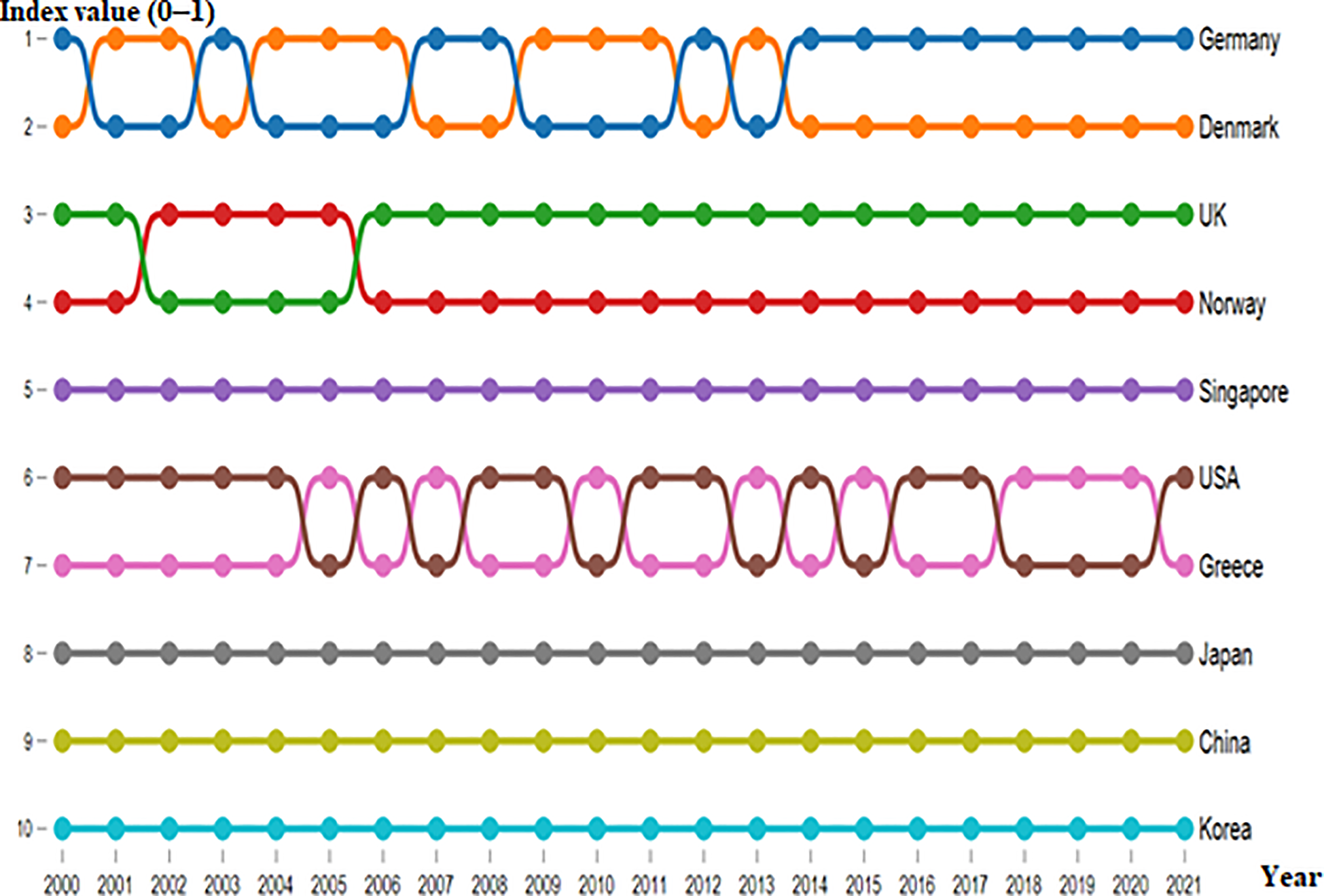
Red index by years.
Table 1
| Variables | Symbol | Definition of variables | Units | Source |
|---|---|---|---|---|
| Dependent variables | TFP | Total fish production | Metric tons | WDI |
| AFP | Aquaculture production | Metric tons | WDI | |
| FGDP | Value added for the agriculture, forestry, and fishing sector | % of GDP | OECD | |
| Independent variables | BIOD | Biodiverty | ındex (0-1) | OECD |
| FD | Financial development | Domestic credit to private sector (% of GDP) | WDI | |
| Control variables | CO2 | CO2 emissions | CO2 emissions (kt) | WDI |
| IQ | Institutional quality | Index | WDI | |
| GDPPER | GDP per capita | current US$ |
Variables.
Econometric model
The model used for the empirical analysis of the study was developed by Ahammed et al. (2025) and Hossain et al. (2024) based on their studies. Three separate empirical models designed in accordance with the purpose of the study are as follows:
In all of the above, Equations 1–3, the natural logarithms of the variables were taken to prevent the possible heteroscedasticity problem of the variables, and elasticities were obtained by using the double logarithmic model. In the models, TFP, AFP, and FGDP are dependent variables; BIOD and FD are the main independent variables; and CO2, IQ, and GDPPER are control variables. To better illustrate the sequential structure of the research design and the relationships among the variables, the analysis flowchart is presented (Figure 5). The extended econometric specifications and robustness models are represented in Equations 4–11, which provide alternative formulations of the main relationships under investigation.
Methodology
Cross-sectional dependence (CD), unit root, and homogeneity
The inclusion of the CD test in panel data econometrics is of great importance. The reason for this, as emphasized by O’Connell (1998), is the potential to obtain biased results in unit root and coefficient estimates if a study is conducted without considering CD. Additionally, the CD test helps make decisions regarding the selection of appropriate tests (first and second generation) in unit root, cointegration, and causality testing processes. Therefore, in this study, the CD test was performed using Breusch and Pagan’s (1980) Lagrange multiplier (LM) test.
Figure 5
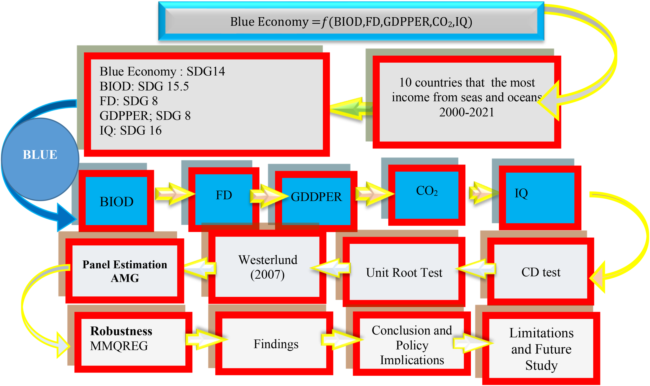
Analysis flowchart.
When the time dimension (T) exceeds the unit dimension (N), the LM test reveals stronger results. The test statistics for LM can be formulated as:
The null hypothesis of the LM test is “There is no CD”, and the alternative hypothesis is “There is a CD”. The test statistic obtained from the LM is then compared to appropriate critical values to detect the presence of cross-sectional dependence.
After CD analysis, a unit root test was performed for the series. In this study, the unit root test was conducted using the CIPS unit root test, which is a second-generation test that takes CD into account. The CIPS test statistic introduced by Pesaran (2007) can be written as follows:
CADFi shows the average of the expanded ADF statistics for each slice. The null hypothesis of the CIPS test is “there is a unit root (the series is not stationary)”, and the alternative hypothesis is “there is no unit root (the series is stationary)”. Critical values for this test are tabulated by Pesaran (2007). These tabulated critical values are compared with the CIPS test statistics to determine whether there is a unit root in the series.
After the stationarity levels of the series were determined, the CD test for the errors obtained from the long-term equation was again carried out with Breusch and Pagan’s (1980) LM test before moving on to the cointegration stage.
Heterogeneity of slope coefficients is another important assumption of panel data models. Many studies imply homogeneity by assuming that slope coefficients do not vary from one unit to another. However, the impact of independent variables may vary between units. Therefore, estimators that assume homogeneous coefficients are likely to produce biased results (Guven et al., 2019). In light of this, before proceeding with the predictions in the study, a test for slope heterogeneity was conducted using delta tests developed by Pesaran and Yamagata (2008). Test statistics for delta tests can be written as:
The null and alternative hypotheses for these tests are presented as “homogeneous slope coefficients” and “heterogeneous slope coefficients,” respectively. A decision is made by comparing the test statistics obtained from these tests with the relevant critical values.
Cointegration test
In this study, the panel cointegration test formulated by Westerlund (2007) was employed to investigate the existence of a cointegration relationship among the variables. This error correction-based (ECM) cointegration test has several important advantages. These include the following: (i) It allows the investigation of the cointegration relationship in the presence of unbalanced panels. (ii) Allowing heterogeneous slope parameters. (iii) It allows CD and obtains solid critical values in the presence of CD. In Westerlund’s (2007) cointegration test, a total of four test statistics are calculated, two for all panels (Pt and Pa) and two for group averages (Gt and Ga). These test statistics can be expressed as follows:
For both test groups, the null hypothesis is expressed as “there is no cointegration”, while the alternative hypothesis is expressed as “there is cointegration”. If the panel shows heterogeneity, it is more appropriate to rely on group statistics, while if it is homogeneous, panel statistics should be given more credence.
Benchmark estimation
Pesaran and Smith (1995) developed the Mean Group Estimator (MG), which is used in estimating panel data models when T is large enough. This estimator is a panel data estimation method used under the assumption of the absence of heterogeneity and CD. If CD is present, the MG estimator may produce biased results. Therefore, in the presence of CD, estimators that take this into account should be used. Based on this, the AMG estimator developed by Eberhardt and Teal (2010) was used in this study.
The rationale behind choosing the AMG estimator lies in its ability to provide consistent and robust estimates in the presence of unobserved common factors that may influence the dependent variable across panels. While Generalized Method of Moments (GMM) and conventional Fixed Effects (FE) or Random Effects (RE) models are commonly used in panel data analysis, they often assume slope homogeneity and may fail to adequately address cross-sectional dependence, particularly in studies involving countries with diverse economic, social, and environmental characteristics. Although GMM is effective for addressing endogeneity and dynamic panel structures, its assumption of homogeneity and limitations under cross-sectional dependence make it less suitable for the context of this study.
The AMG estimator is an estimator that takes CD into account along with a dynamic process common to unit-specific regressions. The process is completed in three stages. In the first stage of the process, pooled first differences regression (FD-OLS) is expanded with T-1 time lag dummy variable coefficients to obtain estimates of the coefficients.
Here = shows the time shadow coefficients. In the second stage , models are estimated by including unit-specific regressions.
In the last stage, the average group estimator is obtained using Pesaran and Smith’s (1995) MG approach:
Here It gives the average of individual predictors obtained using T observations and estimated by the least squares method.
In addition, the Method of Moments Quantile Regression (MMQR) method developed by Machado and Silva (2019) was used to test the robustness of the results obtained from the AMG estimator. Quantile regression was first proposed in the literature by Koenker and Bassett (1978) and makes it possible to detect distributional heterogeneity in the relationship between variables. In addition, this model provides results that are resistant to heteroskedasticity, outliers, and nonnormal distributions and allows its application to evaluate the dependent variance and conditional mean according to the value of explanatory parameters. In this context, this study uses the Method of Moments Quantile Regression (MMQR) proposed by Machado and Silva (2019). MMQR is a more appropriate method when the model has endogenous explanatory variables and panel data are characterized by individual effects (Sarkodie and Strezov, 2019).
In this study, appropriate data econometric techniques were carefully selected considering the characteristics of the data set. Cross-sectional dependence was tested using the Breusch and Pagan (1980) LM test, while stationarity was examined via the Pesaran (2007) CIPS test, which accounts for cross-sectional dependence. The Westerlund (2007) cointegration test was employed to investigate long-run relationships, as it accommodates cross-sectional dependence, heterogeneity, and unbalanced panels. For long-run elasticity estimations, the AMG estimator proposed by Eberhardt and Teal (2010) was used due to its ability to address cross-sectional dependence and slope heterogeneity. Additionally, to test the robustness of the AMG results and capture distributional heterogeneity, the Method of Moments Quantile Regression (MMQR) developed by Machado and Silva (2019) was applied. MMQR is particularly suitable for models with endogenous explanatory variables and panel data with individual effects, providing reliable results even in the presence of heteroskedasticity, outliers, and nonnormal distributions.
Results
In panel data analysis, it is very important to conduct CD tests for both the series and the model. Because the effect of a shock (crisis, flood, fire, etc.) that may occur in one country is likely to affect other countries. Therefore, the results of a study conducted without checking the CD may be biased. In this context, in this study, the CD in the series and models is tested by means of the LM test and reported in Table 1. The results in Table 1 reveal that the null hypothesis of no CD is rejected for all variables except lnTFP and lnAFP. In other words, except for these two variables, the variables considered in the study have CD. Moreover, the results in Table 2 show that CD is also present in the errors obtained from the long-run equation of models 1, 2, and 3. Finally, the homogeneity assumption is also tested for all three models in Table 2, and the null hypothesis of no homogeneity is rejected in all models. Therefore, there is heterogeneity for all models, and appropriate long-run estimators should be selected.
Table 2
| Variables | CD test | Homogeneity | ||||||
|---|---|---|---|---|---|---|---|---|
| Model 1 | Model 2 | Model 3 | ||||||
| CD test | p-value | Delta | p-value | Delta | p-value | Delta | p-value | |
| lnTFP | − 0.889 | 0.374 | 8.772*** | 0.000 | 10.247*** | 0.000 | 5.706*** | 0.000 |
| lnAFP | − 0.861 | 0.389 | 10.624*** | 0.000 | 12.410*** | 0.000 | 6.911*** | 0.000 |
| lnFGDP | 15.683*** | 0.000 | ||||||
| lnBIOD | 20.953*** | 0.000 | ||||||
| lnFD | 2.618*** | 0.000 | ||||||
| lnCO2 | 1.724* | 0.085 | ||||||
| lnIQ | − 1.833* | 0.067 | ||||||
| lnGDPPER | 22.612*** | 0.000 | ||||||
| Mode1 | 3.839*** | 0.000 | ||||||
| Model2 | 7.790*** | 0.000 | ||||||
| Model3 | 2.63*** | 0.000 | ||||||
Cross-sectional dependence and homogeneity.
***1%, and *10%—statistical significance levels.
Since lnTFP and lnAFP variables do not have CD, and all other variables do, it would be more appropriate to evaluate the unit root results for these two variables according to the IPS unit root test and the unit root test for other variables according to the CIPS unit root test. In this context, according to the results of the CIPS panel unit root test presented in Table 3 below, all series become stationary when the first difference I(1) is taken. According to the results of the IPS unit root test, lnFGDP and lnGDPPER are I(0), and all other variables are I(1).
Table 3
| Variables | CIPS | IPS | ||
|---|---|---|---|---|
| I(0) | I(1) | I(0) | I(1) | |
| lnTFP | 1.538 | − 1.325* | − 0.290 | − 5.156*** |
| lnAFP | 0.890 | − 2.062** | − 1.065 | − 10.281*** |
| lnFGDP | − 0.629 | − 3.241*** | − 4.398*** | – |
| lnBIOD | 1.712 | − 2.027** | 2.169 | − 10.992*** |
| lnFD | 0.392 | − 1.317* | − 0.464 | − 5.498*** |
| lnCO2 | 1.321 | − 1.461* | − 0.536 | − 9.833*** |
| lnIQ | 1.554 | − 2.888*** | 0.700 | − 10.611 |
| lnGDPPER | − 0.632 | − 2.301** | − 2.545*** | – |
Unit root test.
***1%, **5%, and *10%—statistical significance levels.
Following the CD test for the model (see Table 2), Westerlund (2007) ECM cointegration test is used to test whether there is a cointegration relationship between the variables. Looking at the Westerlund ECM cointegration test results in Table 4, it is decided that there is a cointegration relationship between the variables in all models according to the robust p-values. Following the confirmation of the existence of a cointegration relationship, long-run parameters were estimated. Before estimating the long-run elasticities, it is tested whether these long-run elasticities vary from unit to unit (see Table 2), and it is concluded that the variables vary from unit to unit in the long run. In other words, there is heterogeneity in the long run. In this context, the recently popular AMG approach, which takes into account both CD and slope heterogeneity, is used to estimate the three models considered in this study.
Table 4
| Statistic | Value | Z-value | p-value | Robust p-value |
|---|---|---|---|---|
| Panel A: Model 1 | ||||
| Gt | − 2.320*** | 2.386 | 0.992 | 0.000 |
| Ga | − 0.461 | 6.453 | 1.000 | 1.000 |
| Pt | − 6.385*** | 2.435 | 0.993 | 0.000 |
| Pa | − 0.691*** | 5.254 | 1.000 | 0.000 |
| Panel B: Model 2 | ||||
| Gt | − 2.407*** | 2.088 | 0.982 | 0.000 |
| Ga | − 0.452 | 6.457 | 1.000 | 1.000 |
| Pt | − 4.875*** | 3.951 | 1.000 | 0.000 |
| Pa | − 0.639*** | 5.272 | 1.000 | 0.000 |
| Panel C: Model3 | ||||
| Gt | − 2.529*** | 1.668 | 0.952 | 0.000 |
| Ga | − 0.371 | 6.484 | 1.000 | 1.000 |
| Pt | − 5.018*** | 6.820 | 1.000 | 0.000 |
| Pa | − 0.717*** | 5.421 | 1.000 | 0.000 |
Cointegration results.
***1%—level of significance.
Table 5 shows the long-run estimation results obtained from the AMG approach for models 1, 2, and 3. According to the results in model 1, the effect of all independent variables on lnTFP in the long run is statistically significant. According to the long-run effects, 1% increases in lnBIOD, lnIQ, and lnGDPPER increase lnTFP by 0.667%, 0.299%, and 0.304%, respectively. However, 1% increases in lnFD and lnCO2 decrease lnTFP by 0.081% and 0.043%, respectively. When the results of model 2 are analyzed, it can be said that the long-run effects of all variables on lnAFP are statistically significant. When the long-run effects are analyzed, it is seen that a 1% increase in lnFD decreases lnAFP by 0.282% and a 1% increase in lnCO2 decreases lnAFP by 0.079%. The effects of lnBIOD, lnIQ, and lnGDPPER on lnAFP are positive and are 0.731%, 0.506%, and 0.385%, respectively.
Table 5
| Variables | Model 1 | Model 2 | Model 3 |
|---|---|---|---|
| lnBIOD | 0.667*** [0.098] | 0.731*** [0.073] | 0.705*** [0.102] |
| lnFD | − 0.081* [0.039] | − 0.282* [0.145] | 0.079 [0.096] |
| lnCO2 | − 0.043*** [0.006] | − 0.079*** [0.010] | − 0.057* [0.026] |
| lnIQ | 0.299* [0.181] | 0.506* [0.261] | 0.397* [0.233] |
| lnGDPPER | 0.304* [0.182] | 0.385* [0.177] | 0.238* [0.105] |
| C | 12.133*** [2.017] | 9.099*** [1.787] | 2.913** [1.284] |
AMG results.
***1%, **5%, and *10%—statistical significance levels.
Finally, the results of model 3 in Table 5 show that all independent variables, except lnFD have a significant long-run effect on the dependent variable lnFDGDP. Accordingly, in the long run, a 1% increase in lnCO2 decreases lnFGDP by 0.057%. In addition, the long-run results reveal that lnBIOD, lnIQ, and lnGDPPER positively affect lnFGDP by 0.705%, 0.397%, and 0.238%, respectively.
Robustness
The robustness test of the long-run elasticities of the AMG estimator is performed with the MMQREG approach and presented in Table 6 below.
Table 6
| Panel A: Model 1 | |||||||||
|---|---|---|---|---|---|---|---|---|---|
| Variables | 0.1 | 0.2 | 0.3 | 0.4 | 0.5 | 0.6 | 0.7 | 0.8 | 0.9 |
| lnBIOD | 1.770* | 1.782** | 1.892*** | 1.910*** | 1.994*** | 1.979*** | 2.010*** | 2.077*** | 2.298*** |
| lnFD | − 0.560** | − 0.611** | − 0.645** | − 0.685** | − 0.787* | − 0.866 | − 0.920 | − 0.940 | − 0.988 |
| lnCO2 | − 1.890*** | − 1.673*** | − 1.531*** | − 1.361*** | − 0.929** | − 0.594 | − 0.363 | − 0.277 | − 0.076 |
| lnIQ | 2.341*** | 2.034*** | 1.833*** | 1.593** | 0.981** | 0.508* | 0.181 | 0.060 | − 0.224 |
| lnGDPPER | − 1.307 | − 1.294 | − 1.286 | − 1.276* | − 1.251** | − 1.232** | − 1.218** | − 1.213** | − 1.201* |
| lnGDPPERsq | 1.06e−10 | 1.36e−10 | 1.56e−10 | 1.80e−10* | 2.41e−10* | 2.88e−10* | 3.21e−10* | 3.33e−10* | 3.61e−10* |
| Panel B: Model 2 | |||||||||
|---|---|---|---|---|---|---|---|---|---|
| Variables | 0.1 | 0.2 | 0.3 | 0.4 | 0.5 | 0.6 | 0.7 | 0.8 | 0.9 |
| lnBIOD | 1.624*** | 1.703*** | 1.750*** | 1.807*** | 1.875*** | 1.902*** | 1.995*** | 2.023*** | 2.097*** |
| lnFD | − 0.731** | − 0.628** | − 0.563** | − 0.485* | − 0.335 | − 0.095 | 0.063 | 0.168 | 0.208 |
| lnCO2 | − 1.288*** | − 1.184*** | − 1.117*** | − 1.039*** | − 0.888*** | − 0.645*** | − 0.485*** | − 0.378** | − 0.338** |
| lnIQ | 1.361*** | 1.162*** | 1.035*** | 0.885** | 0.598 | 0.135 | − 0.170 | − 0.373 | − 0.450 |
| lnGDPPER | − 1.564*** | − 1.565*** | − 1.565*** | − 1.566*** | − 1.567*** | − 1.569*** | − 1.571*** | − 1.572*** | − 1.572*** |
| lnGDPPERsq | 3.44e−10*** | 3.53e−10*** | 3.58e−10*** | 3.64e−10*** | 3.76e−10*** | 3.95e−10*** | 4.07e−10*** | 4.16e−10*** | 4.19e−10*** |
| Panel C: Model3 | |||||||||
|---|---|---|---|---|---|---|---|---|---|
| Variables | 0.1 | 0.2 | 0.3 | 0.4 | 0.5 | 0.6 | 0.7 | 0.8 | 0.9 |
| lnBIOD | 2.230** | 2.259*** | 2.282*** | 2.297*** | 2.316*** | 2.337*** | 2.349*** | 2.362*** | 2.412*** |
| lnFD | − 0.026 | − 0.059 | − 0.067 | − 0.076 | − 0.089 | − 0.102 | − 0.112 | − 0.128 | − 0.147* |
| lnCO2 | − 0.338*** | − 0.314*** | − 0.308*** | − 0.302*** | − 0.292*** | − 0.282*** | − 0.275*** | − 0.264*** | − 0.250*** |
| lnIQ | 0.318 | 0.482** | 0.523*** | 0.564*** | 0.632*** | 0.695*** | 0.745*** | 0.822*** | 0.918*** |
| lnGDPPER | − 1.276*** | − 1.419*** | − 1.454*** | − 1.491*** | − 1.550*** | − 1.604*** | − 1.648*** | − 1.785*** | − 1.799*** |
| lnGDPPERsq | 4.37e−10*** | 4.79e−10*** | 4.90e−10*** | 5.01e−10*** | 5.18e−10 | 5.34e−10*** | 5.47e−10*** | 5.67e−10*** | 5.91e−10*** |
MMQREG results.
***1%, **5%, and *10%—statistical significance levels.
According to the results of model 1 presented in panel A of Table 6, the lnBIOD variable has a positive effect on lnTFP in all cartels, and this effect increases gradually in high cartels. The effect of lnFD on lnTFP is negative and significant in low cartels and negative but statistically insignificant in high cartels. lnCO2 and lnGDPPER variables have a negative and statistically significant effect on lnTFP in all cartels. Finally, lnIQ has a positive and statistically significant effect on lnTFP in low quartiles, while lnGDPPERsq is positive and statistically significant in all quartiles. This finding also shows that there is an inverted U-shaped relationship between GDPPER and blue growth. It is observed that the independent variables have similar effects for the model 2 dependent variable lnAFP in panel B and the dependent variable lnFGDP in model 3 in panel C presented in Table 6. Accordingly, the findings obtained from the AMG estimator for all three models are supported by the findings obtained from the MMQREG approach, implying that the estimation results are consistent.
Discussion
The findings of our study reveal that there is a positive relationship between blue economy indicators and biodiversity. This result implies that blue economy elements will increase with increasing biodiversity. In this context, as stated by Turlakova (2021), with the increase in biodiversity, climate change can be reduced, excessive consumption of natural resources can be prevented, and blue economy elements can be promoted, especially by supporting employment and economic growth. Another result obtained from the study is that increases in financial development negatively affect the blue economy. This result contradicts the findings of Mallin et al. (2019); Pascal et al. (2021); Nham and Ha (2023), and Shan et al. (2023). Our findings imply that the financial assets increased through financial development are not effectively utilized in establishing the blue economy and creating a sustainable marine ecosystem, and accordingly, the funds obtained through increased financial development are not transferred to elements that support the blue economy. Similarly, our empirical findings reveal that increases in CO2 emissions have a negative impact on blue economy elements. This finding suggests that, contrary to Hossain et al. (2024), increasing emission levels degrade the marine ecosystem and threaten the blue ecosystem by damaging marine diversity.
Contrary to the above, the findings from our study suggest that there is a positive relationship between the establishment of institutional quality and the increase in economic growth and the blue economy. This finding suggests that the establishment of institutional quality and increased economic growth can result in an increase in the blue economy without harming the marine ecosystem. In addition, increased institutional quality can be seen as an opportunity to prevent factors that harm the marine ecosystem. These findings from the study are in line with the results of the study of Hossain et al. (2024).
Conclusion and policy recommendations
The aim of this study is to analyze the 10 countries that earn the highest income from the seas and oceans. The countries included in the scope of the analysis are China, Germany, Singapore, Denmark, the UK, Greece, Japan, Korea, Norway, and the USA. In the study, CDS test, unit root test, cointegration test, and long-run estimators were used.
The determination of the positive effect of BIOD and IQ variables on the blue economy shows that the blue economy resources of the country make significant contributions to the national economy if they are managed within a sound institutional framework. It also shows that sustainable management of marine and ocean ecosystems can increase environmental welfare by providing ecosystem services, as well as fisheries, tourism, maritime transport, and other marine and ocean-based industries. Furthermore, this finding suggests that the country can reap economic benefits not only directly from marine and ocean industries but also from environmentally friendly tourism and, with a sound institutional structure, aquaculture trade and other areas. The negative impact of FD on blue growth can be attributed to three reasons. These include the following: (I) financial development is often associated with economic growth and industrialization, which can lead to overuse and pollution of marine and ocean resources; (II) FD encourages the over-exploitation of natural resources, which can result in a decrease in marine biodiversity and damage to marine ecosystems; and (III) FD may lead to the relaxation or disregard of environmental regulations, which can hinder the sustainable management of marine and ocean resources. The fact that the GDPPER variable positively affects the blue economy after a certain point can be explained by the EKC hypothesis. This suggests that the ecosystem is not taken into consideration in the early stages of growth and is considered in the later stages. The effect of carbon emissions on the blue economy can be explained by the impact of CO2 on the ecosystem.
The results obtained in this study show that policymakers also have an important role to play. Firstly, it should be taken into consideration that the blue economy is not only based on tourism, but that fishing activities have an important place in the blue economy. For this purpose, studies should be carried out on endangered fish species, and penal sanctions should be imposed on fishing. Another result shows that, to reduce or eliminate the negative impact of financial development on the blue economy, sustainable financial development that considers the blue economy is necessary. As a result, it is recommended that policymakers develop a sustainable financial and economic growth policy that considers marine or ocean life.
When the limitations of the study are examined, it is seen that this study covers the countries that generate the most income from the seas and oceans and does not examine the remaining countries. This situation indicates that more economies need to be analyzed. In this context, conducting similar studies for different country groups and different time periods will increase the validity and reliability of the results. In addition, although the OECD Red List Index is comprehensive, it may not fully capture marine biodiversity changes, indicating that more specialized indicators should be considered. The analysis also lacks sector-specific insights within the blue economy, and future studies can address this issue by examining industries such as fishing, maritime transportation, and coastal tourism separately.
Statements
Data availability statement
The original contributions presented in the study are included in the article/supplementary material. Further inquiries can be directed to the corresponding authors.
Author contributions
SÇ: Formal Analysis, Writing – original draft, Investigation, Writing – review & editing. EK: Validation, Investigation, Writing – original draft, Data curation. AB: Investigation, Writing – review & editing, Writing – original draft. KA: Writing – original draft, Visualization. AP: Data curation, Writing – original draft, Visualization. AN: Investigation, Conceptualization, Supervision, Writing – original draft, Visualization.
Funding
The author(s) declare financial support was received for the research and/or publication of this article. This study was supported by the Recep Tayyip Erdoğan University Development Foundation (Grant ID: 02025006018555). The authors gratefully acknowledge the Foundation for its support.
Acknowledgments
The authors would like to thank the Ongoing Research Funding Program (ORF-2025-87), King Saud University, Riyadh, Saudi Arabia, for their valuable support.
Conflict of interest
The authors declare that the research was conducted in the absence of any commercial or financial relationships that could be construed as a potential conflict of interest.
Generative AI statement
The author(s) declare that no Generative AI was used in the creation of this manuscript.
Any alternative text (alt text) provided alongside figures in this article has been generated by Frontiers with the support of artificial intelligence and reasonable efforts have been made to ensure accuracy, including review by the authors wherever possible. If you identify any issues, please contact us.
Correction note
This article has been corrected with minor changes. These changes do not impact the scientific content of the article.
Publisher’s note
All claims expressed in this article are solely those of the authors and do not necessarily represent those of their affiliated organizations, or those of the publisher, the editors and the reviewers. Any product that may be evaluated in this article, or claim that may be made by its manufacturer, is not guaranteed or endorsed by the publisher.
References
1
Ahammed S. Rana M. M. Uddin H. Majumber S. C. Shaha S. (2025). Impact of blue economy factors on the sustainable economic growth of China. Environ Dev Sustain27, 12625–12652. doi: 10.1007/s10668-023-04411-6.
2
Alharthi M. Hanif I. (2020). Impact of blue economy factors on economic growth in the SAARC countries. Maritime Business Rev.5, 253–269. doi: 10.1108/MABR-01-2020-0006
3
Bennett N. J. (2018). Navigating a just and inclusive path towards sustainable oceans. Mar. Policy97, 139–146. doi: 10.1016/j.marpol.2018.06.001
4
Benzaken D. Adam J. P. Virdin J. Voyer M. (2024). From concept to practice: Financing sustainable blue economy in lessons learnt from the Seychelles experience. Mar. Policy. Volume 163 May2024, 106072. doi: 10.1016/j.marpol.2024.106072
5
Benzaken D. Hoareau K. (2021). From concept to practice: The blue economy in Seychelles. In The blue economy in sub-Saharan Africa. (Routledge), pp. 141–157.
6
Breusch T. S. Pagan A. R. (1980). The Lagrange multiplier test and its applications to model specification in econometrics. Rev. Economic Stud.47, 239–253. doi: 10.2307/2297111
7
Eberhardt M. Teal F. (2010). Productivity analysis in global manufacturing production. economics series working papers no.515 (Oxford, UK: University of Oxford, Department of Economics).
8
Evoh C. J. (2009). The role of social entrepreneurs in deploying ICTs for youth and community development in South Africa. JoCI5, 1–20. doi: 10.15353/joci.v5i1.2463.
9
Guven M. Calik E. Cetinguc B. Guloglu B. Calisir F. (2019). Assessing the effects of flight delays, distance, number of passengers and seasonality on revenue. Kybernetes48, 2138–2149. doi: 10.1108/K-01-2018-0022
10
Hossain M. A. Islam M. N. Fatima S. Kibria M. G. Ullah E. Hossain M. E. (2024). Pathway toward sustainable blue economy: Consideration of greenhouse gas emissions, trade, and economic growth in 25 nations bordering the Indian ocean. J. Cleaner Production437, 140708. doi: 10.1016/j.jclepro.2024.140708
11
Keen M. R. Schwarz A.-M. Wini-Simeon L. (2018). Towards defining the Blue Economy: practical lessons from pacific ocean governance. Mar. Policy88, 333–341. doi: 10.1016/j.marpol.2017.03.002
12
Keesing F. Belden L. K. Daszak P. Dobson A. Harvell C. D. Holt R. D. et al . (2010). Impacts of biodiversity on the emergence and transmission of infectious diseases. Nature468), 647–652. doi: 10.1038/nature09575
13
Lee K. H. Noh J. Khim J. S. (2020). The Blue Economy and the United Nations’ sustainable development goals: Challenges and opportunities. Environ. Int.137, 105528. doi: 10.1016/j.envint.2020.105528
14
Machado J. A. Silva J. S. (2019). Quantiles via moments. J. Econom.213 (1), 145–173.
15
Mallin M. F. Stolz D. C. Thompson B. S. Barbesgaard M. (2019). In oceans we trust: Conservation, philanthropy, and the political economy of the Phoenix Islands Protected Area. Mar. Policy107, 103421. doi: 10.1016/j.marpol.2019.01.010
16
Morgan P. J. Huang M. C. Voyer M. (2022). Blue economy and blue finance: Toward sustainable development and ocean governance. Manila, Philippines: Asian Development Bank. Available online at: https://www.adb.org/publications/blue-economy-and-blue-finance-toward-sustainabledevelopment-and-ocean-governance (Accessed April 20, 2024).
17
Narula K. Spalding M. J. Thiele T. Potsdam H. J. Dyer J. (2023). Task Force 6 accelerating SDGs: Exploring new pathways to the 2030 Agenda [T20 Policy Brief]. Berlin, Germany: T20 Initiative. Available online at: https://t20ind.org/wp-content/uploads/2023/05/T20_PolicyBrief_TF6_Blue-Economy.pdf (Accessed September 6, 2025).
18
Neergheen-Bhujun V. Awan A. T. Baran Y. Bunnefeld N. Chan K. Dela Cruz T. E. et al (2017). Biodiversity, drug discovery, and the future of global health: Introducing the biodiversity to biomedicine consortium, a call to action. J. Glob. Health7, 020304. doi: 10.7189/jogh.07.020304
19
Nham N. T. H. Ha L. T. (2023). The role of financial development in improving marine living resources towards sustainable blue economy. J. Sea Res.195, (2023) 102417. doi: 10.1016/j.seares.2023.102417
20
O’Connell P. G. (1998). The overvaluation of purchasing power parity. J. Int. Economics44, 1–19. doi: 10.1016/S0022-1996(97)00017-2
21
Organisation for Economic Co-operation and Development (OECD) . (2016). The ocean economy in 2030. (Paris, France: OECD Publishing). doi: 10.1787/9789264251724-en.
22
Pascal N. Brathwaite A. Bladon A. Claudet J. Clua E. (2021). Impact investment in marine conservation. Ecosyst. Serv.48, 101248. doi: 10.1016/j.ecoser.2021.101248
23
Pesaran M. H. (2007). A simple panel unit root test in the presence of cross-section dependence. J. Appl. Econometrics22, 265–312. doi: 10.1002/jae.951
24
Pesaran M. H. Smith R. (1995). Estimating long-run relationships from dynamic heterogeneous panels. J. econometrics68, 79–113. doi: 10.1016/0304-4076(94)01644-F
25
Pesaran M. H. Yamagata T. (2008). Testing slope homogeneity in large panels. J. Econometrics142, 50–93. doi: 10.1016/j.jeconom.2007.05.010
26
Petrea S. M. Zamfir C. Simionov I.-A. Mogodan A. Rahoveanu A. T. Nancu D. et al . (2021). A forecasting and prediction methodology for improving the blue economy resilience to climate change in the Romanian lower danube euroregion. Sustainability13, (21). doi: 10.3390/su132111563
27
Pimentel D. Wilson C. McCullum C. Huang R. Dwen P. Flack J. et al . (1997). Economic and environmental benefits of biodiversity. BioScience47, 747–757. doi: 10.2307/1313097
28
Sarkodie S. A. Strezov V. (2019). A review on environmental Kuznets curve hypothesis using bibliometric and meta-analysis. Sci. Total Environ.649, 128–145.
29
Sarwar S. (2022). Impact of energy intensity, green economy and blue economy to achieve sustainable economic growth in GCC countries: Does Saudi Vision 2030 matters to GCC countries. Renewable Energy191, 30–46. doi: 10.1016/j.renene.2022.03.122
30
Shan S. Mirza N. Umar M. Hasnaoui A. (2023). The nexus of sustainable development, blue financing, digitalization, and financial intermediation. Technol. Forecast. Soc. Change.195, 122772.
31
Shiiba N. Wu H. H. Huang M. C. Tanaka H. (2022). How blue financing can sustain ocean conservation and development: a proposed conceptual framework for blue financing mechanism. Mar. Policy139, 104575. doi: 10.1016/jmarpol.2021.104575
32
Tirumala R. D. Tiwari P. (2022). Innovative financing mechanism for blue economy projects. Mar. Policy139, 104194. doi: 10.1016/j.marpol.2020.104194
33
Turlakova T. (2021). Bioeconomy as an innovative approach to rural development in the context of Common Agricultural Policy in EU. In SHS Web of Conferences120, 01008. Les Ulis Cedex, France, EDP Sciences. doi: 10.1051/shsconf/202112001008
34
United Nations . (2015). World economic situation and prospects 2017. (United Nations). Available online at: https://www.un.org/development/desa/dpad/publication/world-economic-situation-and-prospects-2017/ (Accessed September 6, 2025).
35
Westerlund J. (2007). Testing for error correction in panel data. Oxford Bull. Economics Stat69, 709–748. doi: 10.1111/j.1468-0084.2007.00477.x
36
Wilkinson D. A. Marshall J. C. French N. P. Hayman D. T. (2018). Habitat fragmentation, biodiversity loss and the risk of novel infectious disease emergence. J. R. Soc. Interface15, 20180403. doi: 10.1098/rsif.2018.0403
37
World Bank . (2017). The World Bank Annual Report 2017. Washington, DC: World Bank. Available online at: https://openknowledge.worldbank.org/handle/10986/27986.
38
World Bank . (2024). Agriculture, forestry, and fishing, value added (constant 2015 US$). (Washington, D.C., USA: World Bank). Available online at: https://data.worldbank.org/indicator/NV.AGR.TOTL.KD (Accessed September 6, 2025).
39
World Economic Forum (WEF) (2020). 5 reasons why biodiversity matters – to human health, the economy and your wellbeing. (Geneva, Switzerland: World Economic Forum). Available online at: https://www.weforum.org/agenda/2020/05/5-reasons-why-biodiversity-matters-human-health-economies-business-wellbeing-coronavirus-covid19-animals-nature-ecosystems/ (Accessed September 6, 2025).
40
Yasser M. M. Halim Y. T. Elmegaly A. A. A. (2024). The blue economy effects on EUROMED tourism: forecasting approach. Futur. Bus J.10, 100. doi: 10.1186/s43093-024-00388-4
Summary
Keywords
blue economy, biodiversity, marine ecosystems, sustainable development, financial development, institutional quality
Citation
Çamkaya S, Kaya E, Barut A, Ali K, Pilatin A and Nassani AA (2025) Treasure lying beneath the waters: exploring the deep connections between biodiversity and the blue economy. Front. Mar. Sci. 12:1624071. doi: 10.3389/fmars.2025.1624071
Received
07 May 2025
Accepted
25 August 2025
Published
17 September 2025
Corrected
23 September 2025
Volume
12 - 2025
Edited by
Di Jin, Woods Hole Oceanographic Institution, United States
Reviewed by
Hummera Nawaz, University of Education Lahore, Pakistan
Mai Yasser, October University for Modern Sciences and Arts, Egypt
Updates
Copyright
© 2025 Çamkaya, Kaya, Barut, Ali, Pilatin and Nassani.
This is an open-access article distributed under the terms of the Creative Commons Attribution License (CC BY). The use, distribution or reproduction in other forums is permitted, provided the original author(s) and the copyright owner(s) are credited and that the original publication in this journal is cited, in accordance with accepted academic practice. No use, distribution or reproduction is permitted which does not comply with these terms.
*Correspondence: Abdulkadir Barut, kadirbarut@harran.edu.tr; Abdulmuttalip Pilatin, abdulmuttalip.pilatin@erdogan.edu.tr
†Present address: Kishwar Ali, Advance Research Center, European University of Lefke, Northern Cyprus, Türkiye
Disclaimer
All claims expressed in this article are solely those of the authors and do not necessarily represent those of their affiliated organizations, or those of the publisher, the editors and the reviewers. Any product that may be evaluated in this article or claim that may be made by its manufacturer is not guaranteed or endorsed by the publisher.