Abstract
In the Elbe estuary, a sharp decline in phytoplankton concentration is observed as the river reaches the deep shipping channels of the Port of Hamburg. This collapse significantly impacts the estuarine food web and carbon cycle, shifting the ecosystem from autotrophic to heterotrophic. Previous studies hypothesized that this decline is primarily due to zooplankton grazing. We propose an alternative hypothesis focused on the role of phytoplankton aggregation with inorganic suspended sediments. We present a novel individual-based Lagrangian model of the Elbe estuary. This model couples hydrodynamic, sediment transport, and biogeochemical processes to investigate the influence of aggregation on phytoplankton mortality. By explicitly accounting for the effect of aggregation-induced sinking, our model suggests that over 80% of phytoplankton larger than 50 µm may be lost to light-limitation-induced mortality. Furthermore, the mortality pattern predicted by our model aligns with areas of intense organic matter remineralization in the estuary. These findings underscore the need for estuarine-specific ecosystem models that can capture the complex interplay between physical and biogeochemical processes in these dynamic environments, while demonstrating the potential of Lagrangian methods to provide new insights into the mechanisms shaping estuarine ecosystems.
1 Introduction
Estuaries are typically highly-productive ecosystems and contribute disproportionately to the global carbon cycle, in addition to their role as a source of nutrients and breeding or hatching grounds for marine ecosystems (Cloern et al., 2014; Arevalo et al., 2023). They are also vital for human use, but activities such as dyking, dredging, and fishing impose significant stressors on the ecosystem (Jennerjahn and Mitchell, 2013; Brown et al., 2022; Wilson, 2002). Modern ecosystem management must balance the long-term sustainability of the ecosystem and climate with the economic interests of stakeholders.
The Elbe estuary in northern Germany flows into the North Sea and represents a particularly challenging system to manage. It is an alluvial estuary, characterized by a wide and shallow mouth near the sea, with an average depth of only a few meters. Dykes for land reclamation and flood protection have confined the river to a narrow channel, typically 1 – 2 km wide. Extensive dredging has been conducted to maintain access for increasingly larger vessels to the Port of Hamburg to depths of approximately 20 m. Unlike most other major European ports (e.g., Rotterdam or Amsterdam), Hamburg lies well inland, about 100 km from the coast This results in an abrupt bathymetric transition as the main channel deepens from roughly 5 m upstream of the city to about 20 m in the harbor (see Figure 1). A side effect of the large channel depth are elevated turbidity levels due to higher tidal energy inputs (Weilbeer et al., 2021; Kappenberg and Grabemann, 2001). These levels are further increased due continuous dredging that is required to maintain the channel depth since the latest deepening campaign in 2019.
Figure 1
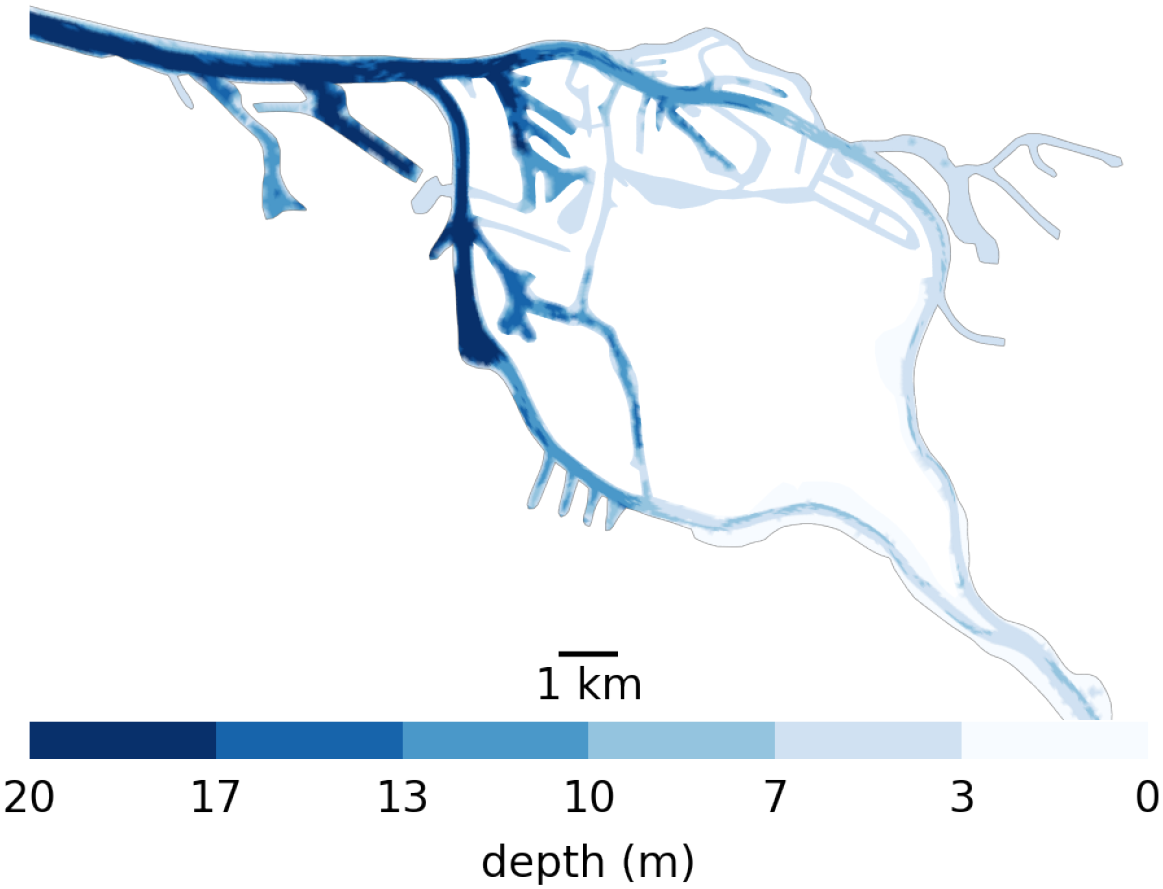
Bathymetry used in the Elbe model around Hamburg. Note, the bathymetry jumps from 5 m upstream (the right-hand side) to 10 m for a short step in the upper port area to 20 m in the lower port area all the way to the North Sea. Also note that there is only one channel to enter the harbor section of the estuary, which is mostly 20m deep from shore to shore. So anything that passes through has to travel through deep water.
Estuarine ecosystem dynamics, like in most ecosystems, are strongly controlled by primary producers, in particular by phytoplankton, which form the basis of the estuarine food web (Chen et al., 2023). Apart from benthic biofilm-forming phytoplankton or microphytopbenthos (Cheah and Chan, 2022), the vast majority of phytoplankton organisms drift passively with the currents. Upon reaching the port the upstream phytoplankton concentrations drop quickly by approximately 90% (see Figure 2). This previously described bathymetric jump is generally thought to be the main cause of the phytoplankton collapse, yet the mechanisms behind this collapse are not fully understood (Schroeder, 1997; Schöl et al., 2014; Holzwarth et al., 2019; Pein et al., 2021). The collapse of the phytoplankton community in the Elbe estuary has been consistently observed since the several decades (Schöl et al., 2014). Looking at this trend over time we see that this effect has increased over recent years and is correlated with the increase in turbidity which has more then tripled since 2010 (Weilbeer et al., 2021) (see Figure 3). Measurements of low oxygen concentrations (<3 mg/l), high ammonium concentrations (15 mmolm−3), and high dissolved inorganic nitrogen downstream of the bathymetric jump suggest a high remineralization rate of organic matter (Sanders et al., 2018; Spieckermann et al., 2022). This is consistent with model results (Schroeder, 1997; Holzwarth and Wirtz, 2018). The high remineralization indicates that upstream phytoplankton is not being diluted or vertically dispersed in a way that allows it to elude the monitoring stations, but is actually dying (Spieckermann et al., 2022; Geerts et al., 2017). A consequence of this phytoplankton community collapse is that the estuary turns from a net autotrophic to a net heterotrophic system during the summer months (Schöl et al., 2014).
Figure 2
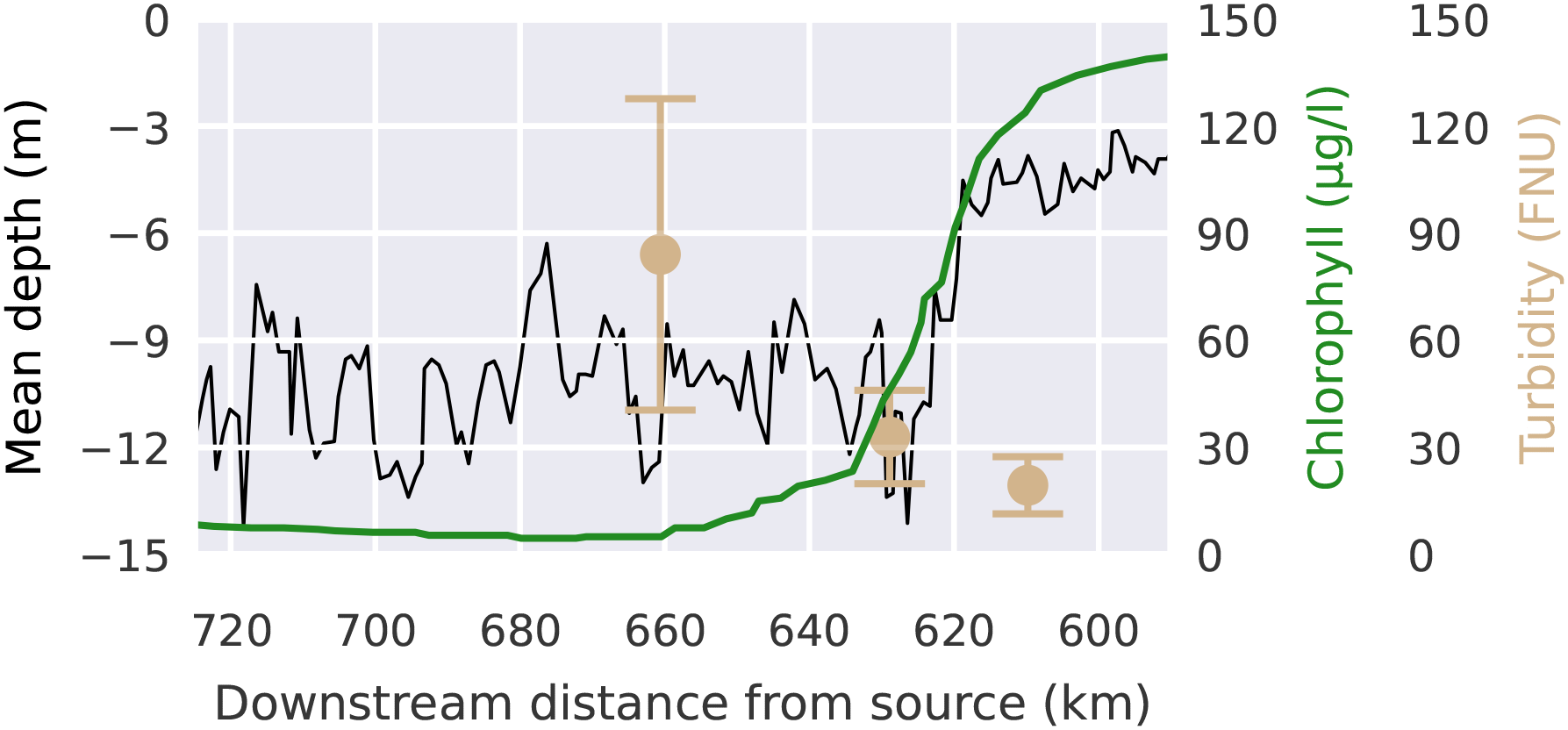
Chlorophyll concentrations as a proxy for phytoplankton biomass (green) and mean depth along a downstream transect averaged from shore-to-shore (black), showing the phytoplankton collapse and correlation with the bathymetric jump. Note, that the x-axis is inverted to keep consistency with the map based plots. Data from (Schöl et al., 2014) and FGG-Elbe https://www.fgg-elbe.de/elbe-datenportal.html (last access: 3 March 2024) presenting the year 2012.
Figure 3
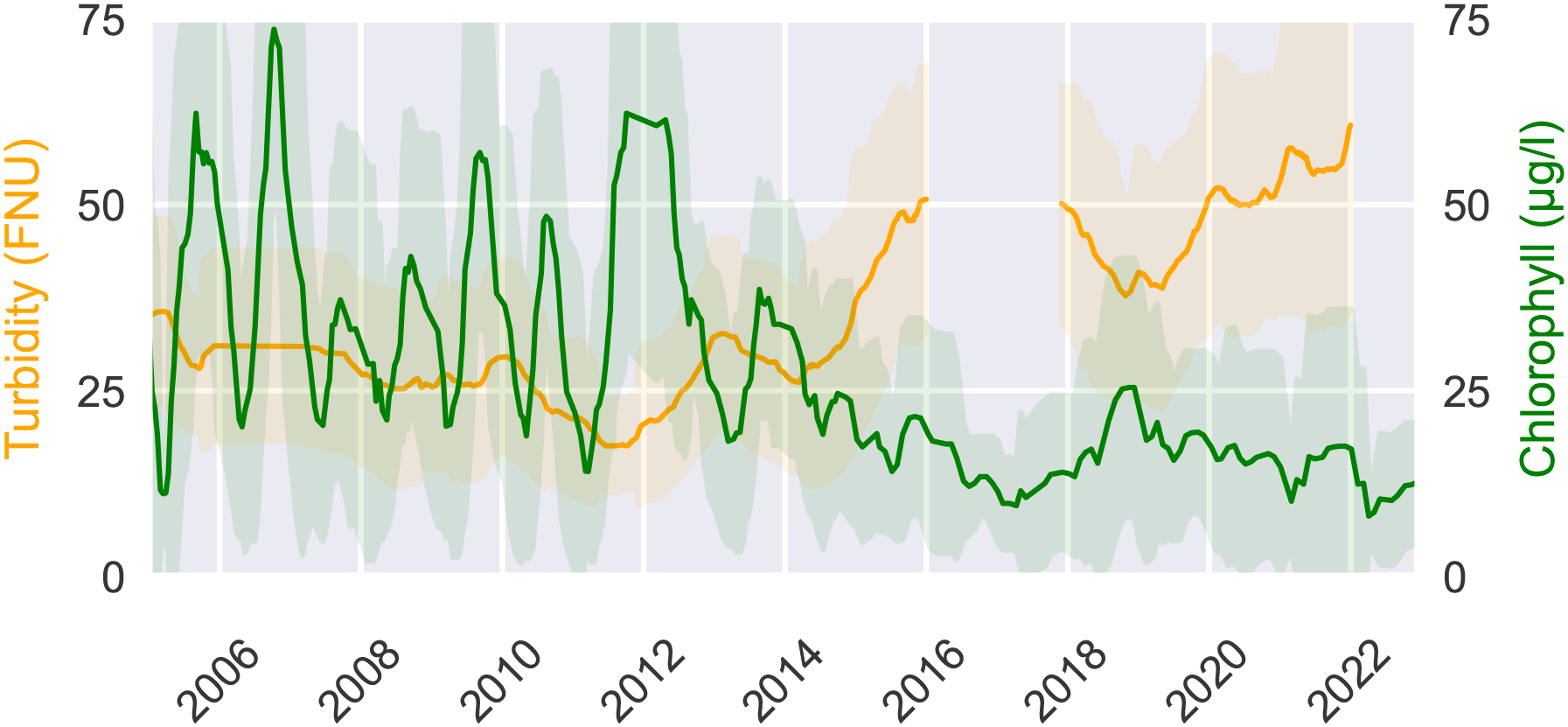
Chlorophyll concentraions as a proxy for phytoplankton biomass and turbidity. Measured from 2005 until 2023 at the station Seemannshöft (Strom-km 628,9) based on data open data available at FGGElbe https://www.fgg-elbe.de/elbe-datenportal.html (last access: 3 March 2024).
Most studies suggest that the phytoplankton collapse in the Elbe is due to grazing or light limitation. The “light limitation hypothesis” is based on the sudden increase in turbidity downstream of the bathymetric jump and the sharp decrease in mean downstream velocity. The latter causes a large increase in residence time. This increase in turbidity in turn increased the aphotic to photic volume ratio, effectively reducing light availability for phytoplankton. Note that the turbidity in the navigational channel is so high that water at a depth of below one meter is aphotic (below 1% of surface light). Both observational and modeling studies suggest that the effect of light-limitation-induced mortality by itself are too slow to explain the sudden drop in phytoplankton concentrations (Walter et al., 2017; Schroeder, 1997). A majority of chlorophyll vanishes within a single day based on water age estimates presented in (Holzwarth et al., 2019; Steidle and Vennell, 2024).
The “grazing hypothesis” assumes that most of the phytoplankton is consumed by zooplankton. A common explanation (Schöl et al., 2014; Hein et al., 2014; Pein et al., 2021) is that marine zooplankton are pushed into the estuary with the tides up to the bathymetric jump. Upstream of the bathymetric jump, the flow velocity is much higher, making it difficult for them to migrate further upstream. This could explain the sudden drop in phytoplankton concentration in this area. Although marine zooplankton species have been observed in the past, Steidle and Vennell, 2024 showed that retention in the area without a sophisticated mechanism is difficult for planktonic organisms. Hence, an accumulation of marine zooplankton to large enough concentrations that could explain this drop in chlorophyll concentrations might not be possible. This suggests that the grazing hypothesis might instead be dependent on upstream freshwater zooplankton that could still easily survive in the low salinity port area. Alternatively, the grazing pressure could be in part due to benthic grazers. With much lower flow velocities close to the bed and a potential ability to hold on or even burry themselves in the sediments they would have a much easier time to persist in that area. Informal reports of there existence have been made but no systematic study has been performed to date to try and quantize their abundance.
The last published zooplankton survey that could be used to examine the effect of zooplankton grazing and therefore the grazing hypothesis has been performed in 1992 (Bernat et al., 1994) and can be considered outdated. At that time of the last survey the bathymetry was significantly different with a narrower navigational channel and a target depth of 13m instead of the current 18m (Hein and Thomsen, 2023). Additionally the upstream biochemistry has changed significantly since the collapse of the German Democratic Republic (GDR). Water quality drastic increased since then causing an increase in in upstream chlorophyll concentrations (Adams et al., 1996; Matthies et al., 2006). First results from a more recent zooplankton survey have been published by Biederbick et al. (2025). However, abundances and or filtration rates necessary to estimate grazing-induced losses are not yet available. This effectively leaves us in the dark about the current impact of grazing on the chlorophyll concentrations.
Another process considered in some models is referred to as “sedimentation” (Hagy et al., 2005; Behzad et al., 2000). This is based on the assumption that individuals in the phytoplankton community have, on average, negative buoyancy. Therefore, they slowly sink, where some of them are assumed to be buried in the sediment. This process is also implemented in two Elbe models presented in (Schöl et al., 2014; Pein et al., 2021). However, this process lacks calibration and validation data in both models. With their choice of sinking losses these processes can be considered negligible compared to grazing losses.
In marine ecosystems phytoplankton is often limited by nutrients availability. However, the Elbe estuary is highly eutrophic, and expected morality rates under nutrient limiting conditions are generally considered to be too slow to explain the collapse (Schöl et al., 2014; Hillebrand et al., 2018; O’Brien, 1974). Hence, we exclude nutrient limitation as reason for the community collapse.
All current Elbe ecosystem models represent phytoplankton mortality as a combination of a non-linear grazing loss function and a linear “natural mortality” or respiration loss function. In those models the processes of “light-limitation-induced mortality” can be interpreted as indirectly represented through the combination of respiration losses and a light-dependent limitation to their growth function. Aggregation processes are not represented in any of the existing models. Furthermore, while several models include zooplankton grazing they also use zooplankton grazing as a tuning parameter such that the modeled phytoplankton concentrations fit the observed trends (Pein et al., 2021; Schöl et al., 2014; Holzwarth et al., 2019). They also lack an SPM model to represent the highly variable light attenuation within the estuary (see Figure 2). Hence, an inference on the grazing induced mortality is not possible by these models, even though it is claimed in several publication (Schöl et al., 2014; Hein et al., 2014; Pein et al., 2021).
We suggest another explanation that has not yet been explored. Phytoplankton produce transparent exopolymer particles (TEP) and excrete polysaccharides (EPS). Several diatom and flagellate species have been shown to produce large amounts of TEP (Kiørboe and Hansen, 1993; Passow and Alldredge, 1995). These gel-likes substances are sticky, promoting the aggregation of phytoplankton cells into larger aggregates both with itself and other particulates Passow et al. (1994); Passow and Alldredge (1995); Engel (2000). Microscopy and field studies showed marine aggregates from phytoplankton blooms visibly embedded and held together by TEP (Alldredge et al., 1998; Kiørboe and Hansen, 1993). This process plays an important role in formation of “marine snow” and the subsequence sinking of surface phytoplankton into deeper water Alldredge et al. (1998). The increased stickiness also enables them to aggregate with suspended inorganic matter (Lai et al., 2018), which has been observed in the Elbe estuary as well (Wolfstein and Kies, 1999; Tobias-Hünefeldt et al., 2024). Such an aggregation would increase the sinking velocity of phytoplankton due to the high density of inorganic sediments. An increase in sinking velocity would shift their vertical distribution to deeper and therefore darker waters, where they would be more likely to be starved of light. A deeper position in the vertical column also reduces the downstream velocity as average velocities toward the bottom are much lower and may even point upstream (Pein et al., 2021) as typical in estuaries. This further skews the speed of the collapse after the bathymetric jump when measured relative to the along channel position rather than residence time. The phytoplankton aggregates would also be more likely to settle on the bottom, further increasing their residence time, while creating an additional loss term due to potential benthic grazing and sedimentation. We therefore suspect that this turbidity induced sinking may be an important factor in the recent increase in the collapse of the phytoplankton community in the Elbe estuary.
Similar aggregation and settling processes, sometimes also referred to as flocculation and precipitation, have already been demonstrated in lab studies (Deng et al., 2019) and observed in the North Sea on the border between Wadden Sea and North Sea (Schartau et al., 2019; Neumann et al., 2019) The North Sea typically shows high organic aggregates concentrations while the Wadden Sea aggregates are shown to be high in inorganic content. At the boundary between the two precipitation can be observed. This is thought to be due to the aggregation of organic and inorganic particulates, which increases their sinking rate.
Such a process has so far not been explored yet, as it is difficult to represent a varying buoyancy in the current Elbe ecosystem models. These are - as it is standard - examining the ecosystem from an concentration-based or Eulerian perspective. In such a model the domain is split into “boxes”, each representing a volume of water at a fixed location. Phytoplankton within these boxes is represented as a homogeneous concentration. In such an approach the life-history of an phytoplankton cell or aggregate is lost after each model time step, as they are mixed with the surrounding cells and assumed to be identical to all the other phytoplankton (Baudry et al., 2018). Therefore, varying buoyancies are difficult to represent consistently over time. Additionally, Walter et al. (2017) found a strong relationship between the duration of light limitation and the net-growth and -loss rates, with net losses only occurring after 12 days without light.
To represent these two mechanism, we shift our perspective from an Eulerian - where we represent fixed volumes - to a Lagrangian one - where we follow phytoplankton on its trajectory through the estuary. This allows us to preserve temporal consistency between model time steps and in return consistently track the aforementioned aggregate size, buoyancy, and light availability. However, in turn we lose the ability to easily track concentration changes of e.g. nutrients or zooplankton. We are therefore no longer able to accurately represent growth processes, and therefore the full ecosystem dynamics. As we are only interested in the mortality terms, that happen over a short time-span, in a region of the estuary in which the population prior to the bathymetric drop effectively is in a steady-state, this is acceptable for our purposes.
The mechanism of particle aggregation in marine environments is a complex topic. It is best researched in the context of open oceans where marine snow is a major pathway in the global carbon cycle and part of global climate forecasting models (Burd and Jackson, 2009; Jackson and Burd, 2015). Advances have also been made studying aggregation in coastal and estuarine environments (Chen and Skoog, 2017; Horemans et al., 2021; Cox et al., 2019). However, aggregates in different environments differ drastically intheir size distribution and composition which in turns stronglyeffects their characteristics like shape, density, stickiness, andsettling velocities (Kriest, 2002; Cael et al., 2021; Laurenceau-Cornec et al., 2020). This makes it hard to generalize aggregation processes. The standard approach is to estimate collision frequencies between aggregates by using so called coagulation kernels (Stemmann et al., 2004; Burd, 2013). These typically use a “fractal radius” to represent the size of coagulating aggregates to account for inhomogeneous dense packing (Stemmann and Boss, 2012). (Jokulsdottir and Archer, 2016) presents the first study using such a coagulation kernel approach to study aggregation processes from a Lagrangian perspective in a 1-D model. Extending this approach to estuarine and coastal environments has been difficult as they generally require 3D models to represent their complex bathymetries. Until the development of the OceanTracker model (Vennell et al., 2021) this was too computationally expensive to attempt.
We will present a novel model study that attempts to draw attention to this issue. With this model we will investigate the effect phytoplankton aggregation processes from a Lagrangian perspective to examine the impact of “turbidity induced sinking” and the resulting light-limitation-induced mortality on the phytoplankton population. Although we have a similar limitation of validation data as the previous studies, we provide first estimates of the relative importance of these processes.
2 Methods
2.1 Lagrangian model
We have further developed the individual-based Lagrangian model OceanTracker (Vennell et al., 2021) and applied it to the Elbe estuary, similar to (Steidle and Vennell, 2024). Particle tracking on unstructured grids was relatively computationally expensive until recently, when OceanTracker (Vennell et al., 2021) improved the performance by two orders of magnitude to the current state of the art. Looking at the problem from a Lagrangian perspective offers several advantages. First, it allows us to reuse computationally expensive hydrodynamic models to model tracer-like objects. This is overall much faster by several orders of magnitude than recalculating the advection-diffusion equation for tracers in an Eulerian model. Second, because we simulate particles individually, we are able to observe their tracks. This makes the interpretation of our results not only intuitive, but also allows us to include individual-based properties and processes that cannot be represented, or only indirectly, in Eulerian models.
2.2 Hydrodynamic data
We use the hydrodynamic data from the latest validated SCHISM model of the Elbe estuary (Pein et al., 2021). This model uses a three-dimensional unstructured grid to represent the entire Elbe estuary from the weir at Geesthacht to the North Sea, including several side channels and the port area (see Figure 4). The model provides us with a node-based mesh containing a range of information such as water velocity, salinity, water level and dispersion. The year represented in this dataset is 2012 with a temporal resolution of 1 hour and a dynamically varying spatial resolution with node spacing ranging from 5 to 1400 m with a median spacing of about 75 m.
Figure 4
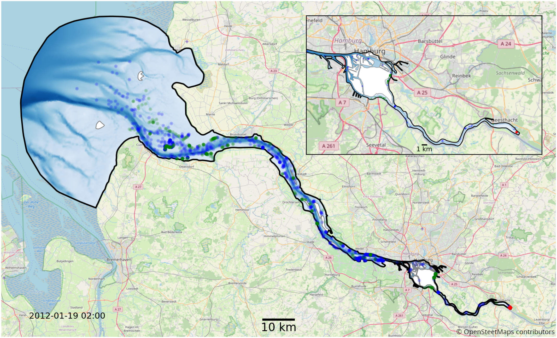
Map of the full model domain, with Geesthacht being the upstream boarder on the right and the North-sea being the downstream border on the left. The black outline marks the edge of the model domain. Blue and green dots show an example snapshot of a fraction of the phytoplankton in the model. The location of the initial release is shown in red. Blue represents floating, green particles stranded by the receding tide. The red area is the initial release location. The background map has been provided by © OpenStreetMap contributors 2023. Distributed under the Open Data Commons Open Database License (ODbL) v1.0.
At the downstream model boundary, the Elbe model was forced by the previously published German Bight model of Stanev et al. (2019) which is based on the AMM7-based CMEMS reanalysis of the northestern European shelf (O’Dea et al., 2017). At the upstream model boundary, river discharge enters the estuary. Daily discharges were derived from observations at the tide-free gauge station at Neu Darchau, made available by FGG Elbe (www.fgg-elbe.de/elbe-datenportal.html). The modeled year (2012) represents a typical year, i.e., discharges were not significantly different from the long-term average. The long-term average discharge is 710 ± 471m3s−1, while yearly average discharges for 2012 were 636m3s−1.
2.3 Suspended particulate matter data
Suspended particulate matter data has been provided by the SediMorph model (Malcherek et al., 2005) developed by the German Federal Waterways Engineering and Research Institute (Bundesanstalt für Wasserbau, BAW). SediMorph is coupled to the hydrodynamic model UnTRIM and provides data on the concentration of suspended particulates for five different size classes (see Table 1).
Table 1
| Sediment type | −log2[mm] | d[µm] |
|---|---|---|
| Fine sand | > 3 | 128–256 |
| Very fine sand | > 4 | 64–128 |
| Coarse silt | > 5 | 32–64 |
| Medium silt | > 6 | 16–32 |
| Fine silt | > 7 | 8–16 |
| Very fine silt | > 8 | 4–8 |
SediMorph size classes and their corresponding size ranges.
The data was provided based on simulations for the year 2016 as a monthly average with a horizontal resolution ranging from 10 to 1000 m. It is based on approximately 100.000 horizontal nodes covering both the Elbe and Weser with a constant 1 m vertical resolution. The data was interpolated to the SCHISM grid as depth averaged values using a barycentric interpolation for the horizontal layer.
In this study we continuously release phytoplankton aggregates representing a subset of the incoming upstream phytoplankton population at the weir in Geesthacht. We then examine how the population distributes throughout the estuary by following their trajectory and, most importantly, their cause of death. As we are primarily interested in their cause of death and the mechanism behind hit we will be ignoring many other biological processes like cell growth and division.
2.4 Phytoplankton mortality causes
Mortality is induced by high salinity or light-limitation. When particles are exposed to salinites above 20 PSU, a mortality probability of 0.5% per minute is imposed. This threshold is chosen based on a range of the salinity tolerances of estuarine phytoplankton species presented in (von Alvensleben et al., 2016). This is only an approximation and salinity tolerances many estuarine phytoplankton species deviate from this. However, the main motivation for this choice is that most of the particles that die through this process have passed the isohaline for more than 12 hours, one tidal cycle, and are assumed not to return again through this isohaline. Anything outside the 20 PSU isohaline is not considered part of the estuary for the purposes of this study. Therefore, we are not tailoring our salinity tolerance to a specific species, but rather testing whether they can retain themselves within this isohaline. This salinity induced mortality also allows us to reach a steady state population size, required to compare upstream and downstream populations easily.
Light limitation is modeled based on observations presented in Walter et al., 2017. They showed that phytoplankton can survive for several days with little or no light before the population starts to decline. To represent this, we model phytoplankton cells with a light budget. This light budget is represented as a moving average of their past illumination. Illumination is calculated once a minute at their current water depth. The moving average () of the local irradiance Iaat step t is calculated using Welford’s online algorithm (Welford, 1962) (Equation 1).
T is the number of averaging time steps. Walter et al., 2017 showed that cell number growth rates during illumination and cell number death rates during darkness differ by about an order of magnitude. To compensate for this, we calculate the light budget using the maximum of two moving averages. The light budget is then calculated as Equation 2
where Td is set to 12 days and Tg is set to 1/10 of Td, which allows them to recover from light limitation faster than they are starved of light. When the light budget decreases below a threshold of 30 Wm−2, the cells are considered light-limited and die with a probability of approximately 3.5 × 10⁻⁵ min−1 (Walter et al., 2017). A sensitivity of this threshold is examined in the supplemental data.
The surface light intensity or irradiance is modeled using the pvlib library (Anderson et al., 2023). We use pvlib to calculate the irradiance field based on the position of the sun relative to the location and time of year, assuming a clear sky. The surface irradiance is then attenuated by the turbidity of the water column using the Beer-Lambert law (Equation 3)
where I(z) is the irradiance at depth z, I0 is the surface irradiance, αa is the surface albedo, ϵ is the attenuation coefficient, c is the turbidity based on the SPM concentration and z is the depth. The surface albedo is set to 0.1 and the chosen attenuation coefficient is 0.15 m−1.
2.5 Aggregation induced buoyancy changes
We represent turbidity induced buoyancy by estimating particle collision and coagulation rates between the phytoplankton cells and the suspended particulate matter. Typically three processes are considered when representing aggregation processes between organic and inorganic particles in marine environments: differential sedimentation, turbulent shear, and Brownian motion. Brownian motion can be neglected in our case because its effect is several orders of magnitude smaller for the size classes that we are considering. Differential sedimentation represents the potential for particles to aggregate based on different settling velocities causing relative motion between the particles, causing them to potentially collide. Turbulent shear represents the potential of particles to aggregate based on relative motion due to shear or small scale turbulence. We refer to these coagulation processes as different coagulation kernels. These kernels can be represented in a rectilinear or curviliniear way. The latter accounts for particles avoiding each other due the changes in the local flow field that the particles themselves cause while the first does not. The curviliniear kernels for turbulent shear and differential sedimentation are defined by Equations 4, 5
where ϵ is the turbulent kinetic energy dissipation rate, ν is the kinematic viscosity of the fluid, p is the particle size ratio ri/rj, ri and rj are the radii of the particles, vi and vj are the sinking velocities of the particles (Burd, 2013). Turbulent kinetic energy dissipation rate and kinematic viscosities are calculated and provided by the SCHISM model.
Estimating particle sinking velocities for aggregated particles is difficult as particle shape, size, and density can vary significantly between different aggregates. The classical approach using the Stokes law, which assumes that aggregates are spherical and homogeneously dense been show to be inadequate for complex marine aggregates as it drastically overestimates the sinking velocities (Kriest, 2002; Cael et al., 2021; Laurenceau-Cornec et al., 2020). Data availability for aggregates composition and size distribution is typically limiting in coastal environments that makes it difficult to apply tailored models. For our case we chose to use an empirical model presented by Kriest (2002). Here sinking velocities are calculated based on a power law and the fractal radius. While there are many other potential models to represent the sinking velocities of aggregates, we found this to be the most suitable as it has been successfully applied in a modeling study already (Kriest, 2002) and because it is tuned to best represent dense phytoplankton-based aggregates.
Sinking velocities are calculated using Equation 6
d is the diameter of the aggregate, B and ν are fitting constants. Based on the “dense Phytoplankton aggregation model” (dPAM) presented in Kriest (2002) they are set to 942d1.17md−1.
We assume that aggregates are sticky due to their exudates. This makes their stickiness proportional to the organic content. We therefore model the stickiness using the ratio of organic to inorganic content presented in (Jokulsdottir and Archer, 2016). The total particle coagulation rate is then calculated by Equation 7
where αs is the maximum sticking probability of particles upon collision for a completely organic aggregate, Vo and Vi are the volumes of organic and inorganic content in each aggregate, and and are the curvilinear coagulation kernels for turbulent shear and differential sedimentation (Burd, 2013). The amount of individual coagulations for each time step is then calculated based on the coagulation probabilities using a Poisson distribution.
Aggregate radius after collision is calculated assuming volume conservation (Equation 8)
where ra is the radius of the aggregate, rSPM is the radius of the SPM particle, and n is the number of SPM particles that collided with the aggregate (Burd and Jackson, 2009).
2.6 Settling and resuspension
We include a settling and resuspension model to represent tidal stranding and particles settling on the bed of the estuary. Particles become stranded when the current grid cell becomes dry. They are not allowed to move from wet cells to dry cells, by the random walk dispersion applied to all particles. A grid cell is considered dry based on the flag given in the SCHISM hydrodynamic model output. Once this cell is rewetted all stranded particles resuspend and are able to move again. Particles settle on the bed once they attempt to move below the bottom model boundary and are resuspended based on a critical shear velocity. The velocity profile in the bottom layer, or log layer, is calculated by Equation 9
where U is the friction velocity representing the drag at height z above the seabed, κ is the van Karman constant, z0 is a length scale reflecting wp the bottom roughness, and u∗ is the critical friction velocity [see Equation 5.5 in Lynch et al. (2014)]. If the velocity is above the critical friction velocity the particle is resuspended. We chose a critical friction velocity of 0.009 ms−1 based on data presented in Carvajalino-Fern´andez et al. (2020) (see supplements for details).
2.7 Diffusivity
Particles are not only advected but also dispersed based on eddy diffusivity. This allows us to implement a dynamic dispersion that is crucial to represent tidal-pumping processes. Dispersion was modeled with a random walk using a random number generator with a normal distribution. The displacement by vertical dispersion ∂z of particle i is calculated following (Yamazaki et al., 2014) as Equation 10
where zi is the vertical position of the particle, is the vertical eddy diffusivity gradient, Kv is the vertical eddy diffusivity provided by the SCHISM model and N is the normal distribution. The term based on is needed to avoid particle accumulation on the top and bottom of the water column from the hydrodynamic model output. Horizontal eddy diffusivity data was not present in the hydrodynamics dataset. Hence, we used an average value to approximate it. The typical values in the literature range form 0.1 − 10 m2s−1 (Sundermeyer and Ledwell, 2001; Bogucki et al., 2005; Viikmäe et al., 2013). With the lower values appropriate for the fine spacial scales examined here we chose 0.1 m2s−1 for our simulations.
2.8 Implementation details
For each particle we record their distance traveled, age, water depth, and status (whether they are drifting or settled on the river bank or bottom). These variables are recorded every 12 hours starting at midnight.
Model simulations and visualizations were performed in Python making heavy use of Numba, a LLVMbased Python JIT compiler (Lam et al., 2015) to significantly speed up the simulations (Vennell et al., 2021). Trajectories were calculated using a second order Runge-Kutta scheme with a fixed time step of 60 seconds. Flow velocities were interpolated linearly in time and space using barycentric coordinates, with the exception of water velocity in the bottom model cell, where a logarithmic interpolation is used in the vertical (law of the wall).
2.9 Experimental configurations
Conceptually, we run two types of experimental setups, one with aggregation and one without. These experiments are accompanied by a series of sensitivity analyses to compensate for the lack of calibration data. We model our population for a period of 1 year. This duration is considered reasonable because it covers the full seasonal cycle and is much longer than the average exit or flushing time of the estuary (see supplements for details). We release 10 individuals per minute for one year at the weir in Geesthacht, resulting in approximately 5 million individuals per case, with approximately 50,000 individuals simultaneously alive. This corresponds to an approximate 1:1 ratio of simulated phytoplankton cells to mesh nodes in the hydrodynamic model at each time step. The released individuals are homogeneously distributed in a volume covering the entire water column at the Geesthacht weir (bottom right in Figure 4).
We also perform a number of sensitivity analyses to account for a lack of validation data. Most importantly, we test a range of different coagulation rates by tuning the sticking probability between 0 and 1 in steps of 0.1. We also test a range of light-limitation-induced mortality rates by tuning both the required average illumination threshold between 10W and 100W and the mortality rate between 0.03% and 0.0003% per minute when below this threshold.
We will compare the model using two metrics. As we are using a Lagrangian model, we can track the fate of each individual particle, particularly its cause of death. To compare the relative importance of different mortality causes, we analyze the relative number of aggregates dying from each cause across different model configurations, e.g., with and without aggregation. The second metric used is the horizontal distribution of death locations. To visualize these distributions, we divide the model domain into equally sized hexagons. The color of each hexagon indicates the number of phytoplankton aggregates that have died in that particular bin. We use these distributions to compare the along-stream alignment of death locations with the observed oxygen minimum zone, which is generally considered to be caused by the remineralization of dead upstream phytoplankton. For this metric, we will present the results for a stickiness of 1 for reasons discussed in the discussion section.
Computations were performed on the supercomputer Mistral at the German Climate Computing Center (DKRZ) in Hamburg, Germany. The simulations were performed on a compute node with two Intel Xeon E5 – 2680 v3 12-core processor (Haswell) and 128 GB of RAM with a total run time of approximately 4 hours.
3 Results
3.1 Relative cause of death
The relative cause of death of phytoplankton aggregates is shown in Figures 5 and 6 for a range of sticking probabilities. A sticking probability αs of zero represents the case without aggregation. In the following we will present the results observed throughout the summer months (April-September) while assuming initial aggregate diameters of 10, 50 and 100 µm while focusing on the 50 µm case as the default. (An analysis examining the sensitivity regarding the light limitation parameterization can be found in the supplements).
Figure 5
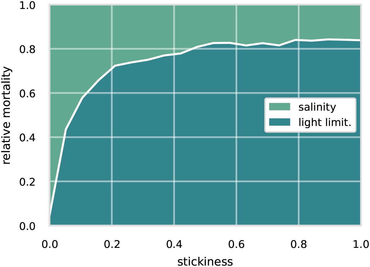
Relative cause of death for a range of stickiness parameterisations for an initial aggregate size of 50 µm.
Figure 6
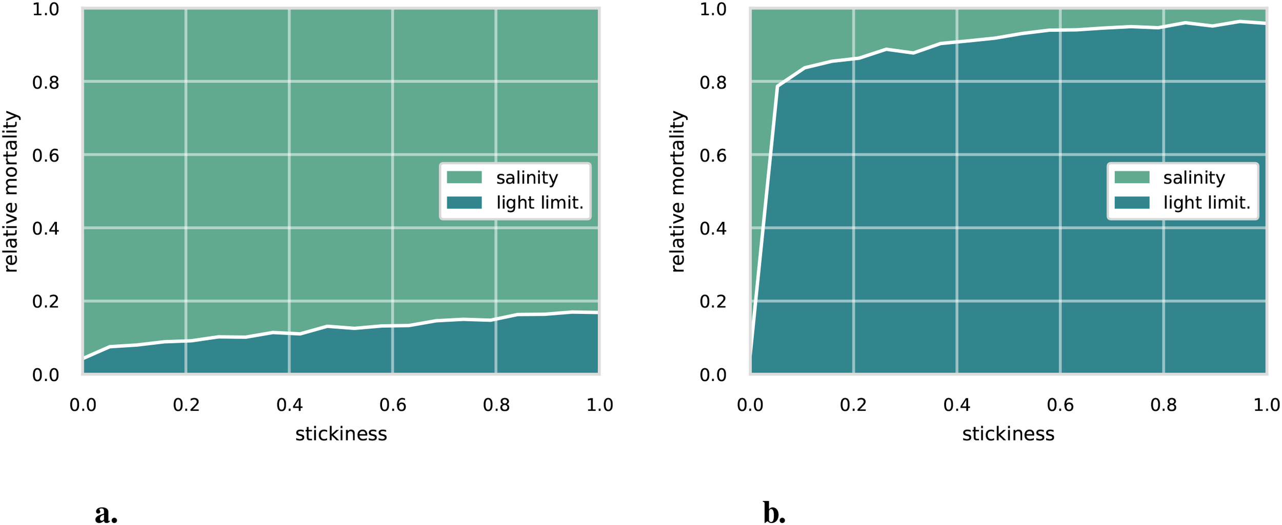
Relative cause of death for a range of stickiness parameterization for an initial aggregate size of (a) 10 µm and (b) 100 µm.
For the 50 µm non-aggregation case (see Figure 5), i.e. stickiness of zero, the main cause of death is salinity with losses due to light limitation around 4%. Implying that most particles are advected out of the estuary’s 20 PSU isohaline. With an increase in sticking probability, we see a shift in the cause of death toward light limitation. For a sticking probability of 0.2, light limitation increases to around 53% and finds its maximum around 80% at a sticking probability of 1. Starting at around 1% for the non-aggregating case, it increases to around 28% for a sticking probability of 0.2 and remains at that level for a sticking probability of 1.
Comparing the 50 µm case to the 10 µm and 100 µm cases (see Figure 6), we see a large sensitivity to the initial aggregate size. The importance of light limitation increases quickly with initial aggregate size. For the 10 µm case, light-limitation induced mortality is below 20% for all sticking probabilities with salinity induced mortality causing 95% of deaths. Also, note the slow increase in light-induced mortality with increasing sticking probability, compared to the 50 µm or 100 µm cases, rising from approximately 4% at a sticking rate of 0 to just over 17% at a sticking rate of 1. For the 100 µm case, light-limitation induced mortality rapidly increases with sticking probability, reaching over 80% of the total mortality at a sticking probability of 1.
3.2 Spatial analysis
We now analyze the horizontal distribution of aggregate deaths with a hexagonal heatmap. Figure 7 shows the location of death for the non-aggregating and aggregating cases during the summer months (April-September), for non-aggregating case (top) and aggregating case (bottom). Both presented cases assume an initial aggregate size of 50 µm and a stickiness of 1. The brightness of the color in each hexagon indicates the relative amount of phytoplankton aggregates dying at that location. Note the difference in scale between the two figures, with the non-aggregation case ranging up to 1% and the aggregating case up to 12%. Hexagons where no aggregate died within the summer months are not colored.
Figure 7
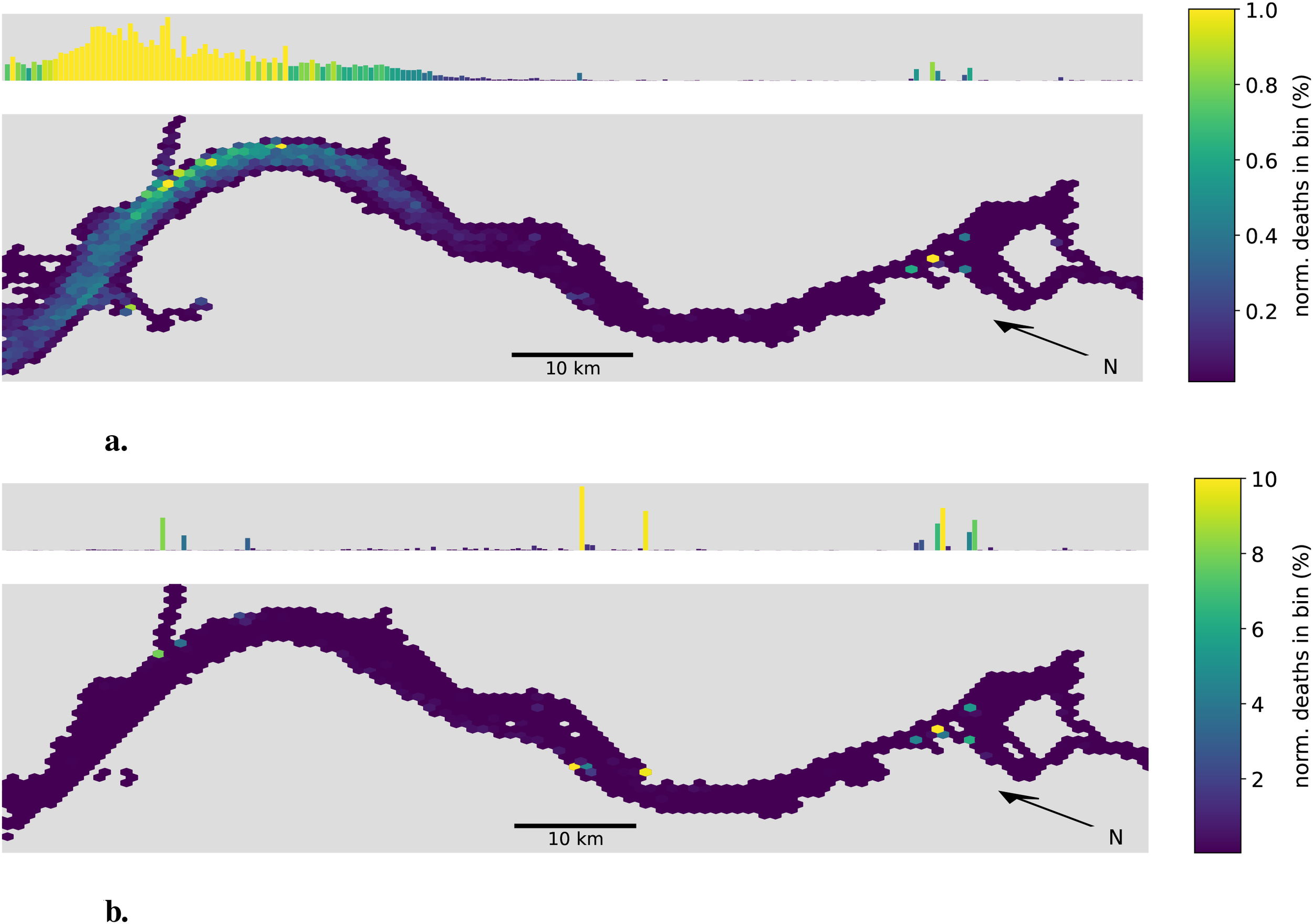
Hex-bin heatmap of the location of death for the summer months (April-September). (a) Non-aggregating case. (b) Aggregating case. The Hamburg port area is located on the right with the North Sea to the left. Both cases assume an initial aggregate size of 50 µm and a stickiness of one. The horizontal map uses colors to indicate the relative amount of phytoplankton aggregates dying within that location bin. Above each horizontal map, a histogram shows the projection on the along-channel axis. Note the different scales.
Comparing the two, we see a clear shift in the location of death. For the non-aggregating case, the main area of high mortality is located close to the mouth of the estuary with its peak close to Brunsbüttel. Note that this area coincides not only with a sharp increase in salinity but also in turbidity and is often referred to as the maximum turbidity zone. A second but significantly less pronounced area of high mortality is located shortly after the bathymetric jump in both the Norder and Süderelbe.
For the aggregating case, we see a shift in the location of death away from the maximum turbidity zone toward the bathymetric jump where the majority - approximately 25% - of all aggregates die. A second area of high mortality is located close to the city of Stade where two harbor bays seem to act as a sediment trap in our model. The previously observed area of high mortality around the turbidity maximum zone is now less pronounced. While it accounted for over 90% of the mortality in the non-aggregating case, it now accounts for less than 20% of the mortality in the aggregating case.
In Figure 8 we take a closer look at the high mortality regions in the Port of Hamburg. We see three distinct high-mortality locations. All three are located within harbor bays, namely from west to east Köhlfleet-, Waltershofer-, Hansa- and Sandau-, and Steinwerder-Hafen. Taking a look at the outer end of the estuary, we also see a difference in the locations where no phythoplankton died in our model (shown in gray). Notably, the tidal flats are largely empty in the aggregating case, with almost all deaths occurring within the deeper sections of the estuary.
Figure 8
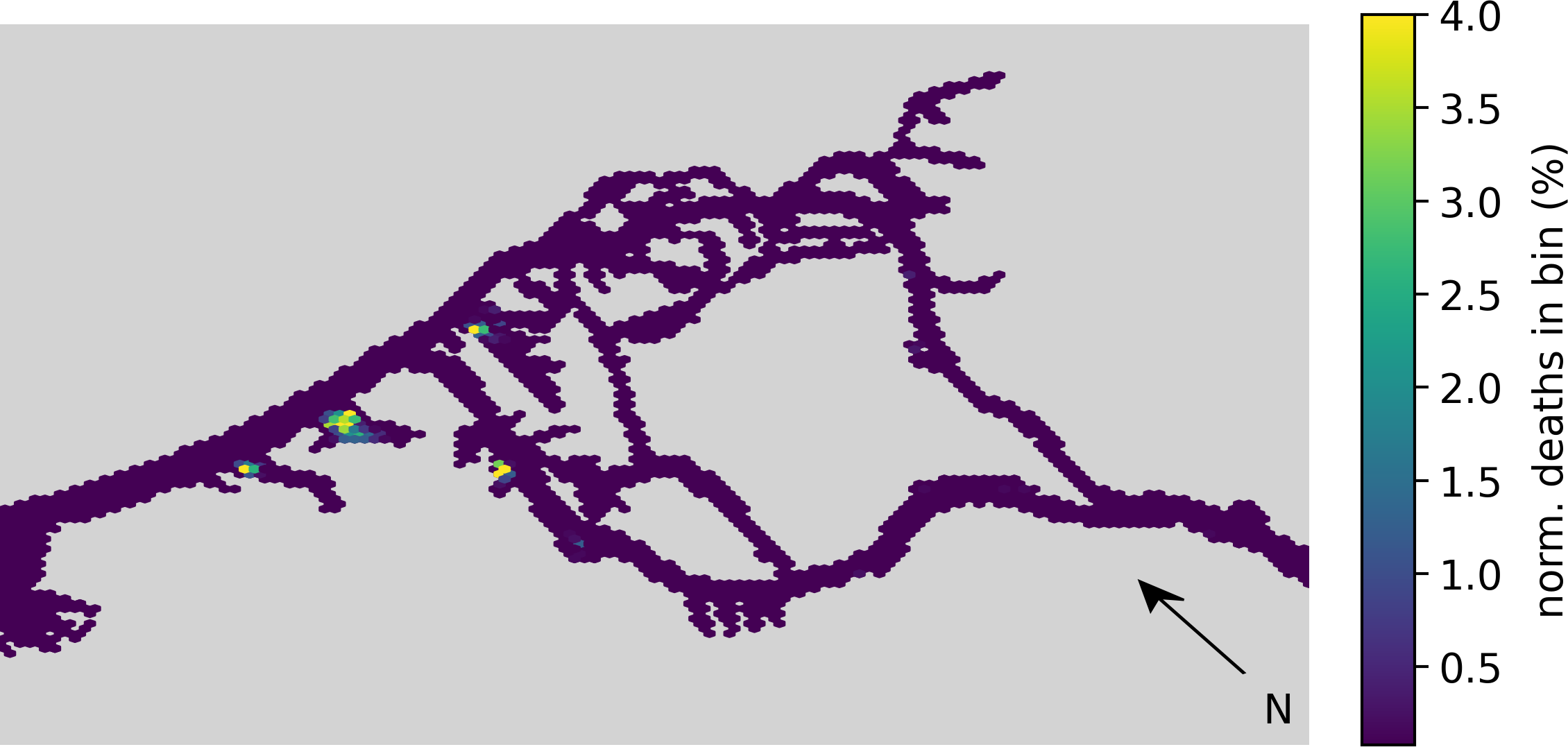
Hex-bin heatmap of the location of death for the summer months (April-September) showing the aggregation case at the Port of Hamburg (previously shown on the very right of Figure 7).The horizontal map uses colors to indicate the relative amount of phytoplankton aggregates dying within that location bin.
4 Discussion
4.1 Interpretation and contextualization of the results
In this study, we examined the effect of aggregation processes on phytoplankton mortality in the Elbe estuary. Primarily, we focused on buoyancy changes due to aggregation with inorganic suspended particulate matter, which are suspected to increase mortality rates due to light limitation. We found that aggregation processes can significantly increase light-limitation-induced mortality by over an order of magnitude (as shown in Figure 5). These results were consistent with observed changes in the location of death. The main location of death for phytoplankton aggregates, when accounting for buoyancy changes due to aggregation with suspended inorganic matter, was found to be shortly after the bathymetric jump. This finding is consistent with other studies examining the phytoplankton community (Pein et al., 2021; Schöl et al., 2014; Schroeder, 1997). The harbor bays in particular are known to be sediment traps. The BfG (Bundesanstalt für Gewässerkunde) and HPA (Hamburg Port Authority) reported that these areas require high dredging volumes to maintain their depth (Fiedler and Leuchs, 2014; Authority, 2015), while Pein et al. (2021) reported high concentrations of dissolved nitrogen within these bays, indicating high remineralization of organic matter. In addition, a recent study modeled sustainable adaptation scenarios in order to examine how fine sediments could be reduced in the port (Pein et al., 2025). The results are also consistent with a recent taxonomic study (Martens et al., 2024). It showed that the large centric diatoms, which make up the majority of the upstream phytoplankton biomass, exhibit a negative correlation with the downstream position in the estuary. After the bathymetric jump, the composition shifts toward flagellates with the potential for mixotrophy and picophytoplankton (phytoplankton < 3 µm in size), both of which are assumed to be underrepresented in microscopic studies. In the context of our study, the centric diatoms are typically closer to a 100 µm size class as shown in Figure 6b, while the small picophytoplankton are closer to the 10 µm size class represented shown in Figure 6a. Hence, we suggest that the observed shift in the phytoplankton community composition might partly be explained by the increased light-limitation-induced mortality of larger diatoms, the ability of mixotrophic flagellates to actively migrate within the water column, and their capacity to withstand darkness for longer periods due to their mixotrophic potential.
In our study, we tested a range of sticking probabilities ranging from zero to one, i.e., from non-aggregating to always aggregating upon collision. Models representing aggregation that do not distinguish the content of aggregates typically work with sticking probabilities between 0.1 and 0.5 (Burd, 2013; Karakaş et al., 2009; Kriest, 2002), while the models that distinguish between organic and inorganic content use a sticking probability of 1 (Jokulsdottir and Archer, 2016). Hence, we argue that for our case the sticking probability of 1 is the most realistic as well.
With the increase in depth, the volume for a cross-section segment increases significantly, which could lead one to conclude that the decrease in concentration is due to dilution. However, dilution requires mixing. In this case, it would require mixing the upstream high-chlorophyll freshwater with other low chlorophyll waters. Because there are no significant tributaries that could dilute the upstream water with other freshwater, the only water that could mix with the upstream water is from the North Sea. While the North Sea water shows a lower chlorophyll concentration than the riverine water, it is also highly saline, with a salinity above 30 PSU. Hence, any mixing is expected to be visible in the salinity concentrations. Because the collapse happens in a freshwater section of the estuary, with salinities below 0.1 PSU, we do not expect dilution with seawater to account for the observed decrease in chlorophyll. However, our model design is currently not able to confirm this hypothesis.
Initially, we were surprised to observe how little light limitation contributed to mortality in the non-aggregating case. By examining the vertical velocities and locations of the aggregates, we found that they were traveling up and down the water column frequently, regularly reaching the surface where they could recover from light limitation. This is consistent with the general understanding of the Elbe estuary as a mostly well-mixed system. While the time spent at the surface is typically short and does not allow for much primary production, it seems to be sufficient to prevent light-limitation-induced mortality in our model.
4.2 Limitations
A major limitation of our study is the lack of grazing representation in our model. We would have liked to include a grazing model to directly compare the suggested light-limitation losses to grazing losses. This could be achieved either by coupling our particle tracker to an established Eulerian ecosystem model or by explicitly representing zooplankton and their grazing within the particle tracker. The former approach would require a two-way, i.e. “online”, coupling between the particle tracker, hydrodynamics, and ecosystem model - a challenging task that was beyond the scope of this study. The latter approach, incorporating zooplankton directly into the Lagrangian framework, was not feasible due to the previously noted lack of zooplankton data. Moreover, no published studies to date have represented zooplankton grazing from a Lagrangian perspective from which default parameter values could be adopted. We hope that this study can motivate further work that includes an aggregation model into the existing Eulerian models to directly compare light limitation losses to grazing losses.
Another limitation of our study is the uncertainty in the sinking velocities of the phytoplankton aggregates. As we highlighted in the methods section, the sinking velocities are based on a model by Kriest (2002). However, there are many other potential models to represent the sinking velocities of aggregates, as presented in (Cael et al., 2021; Laurenceau-Cornec et al., 2020). These different models can vary by an order of magnitude in their sinking velocities, making this a major source of uncertainty in our model.
The choice of coagulation kernel, whether to use a rectilinear or curvilinear kernel, also has a large effect on the effective coagulation rates. (Burd, 2013) compared the effects of these kernels on coagulation rates and showed that they can differ by several orders of magnitude, with the difference becoming more pronounced for larger aggregate size differences (see supplements). We chose to use the curvilinear kernels as they are generally assumed to be more accurate and also represent a more conservative estimate of the coagulation rates.
In Figure 8 we report particle accumulation within the harbor bays and local depressions. Note, that our model does not represent bathymetric changes due to these accumulations. We assume that by including such changes to the bathymetry we would see a more spread out accumulation pattern as local depressions would fill up. Further note, that this accumulation pattern suggest that the denser phytoplankton aggregates spend most of their time either on or close near the bottom where they repeatedly settle and resuspend until they reach a quiescent area. In contrast, the lack of such an accumulation pattern suggest that the non-aggregating phytoplankton stay in suspension. This bedload transport observed in our model of the aggregating phytoplankton might be indicative of a potentially large sensitivity to the resuspension scheme and particularly to the critical friction velocity.
Another process that we neglect is the deaggregation of the phytoplankton aggregates. Shear and turbulence can cause the breakup of aggregates into smaller particles, which limits their size since they are more likely to deaggregate the larger they become. This would be an interesting process to examine in our model, especially because we represent sinking speeds based on aggregate size. However, deaggregation is even less understood than aggregation, with next to no applicable data available. While some marine snow aggregation models include deaggregation processes, they represent them as fixed deaggregation rates or fixed upper size limits in a zeroth-order approximation (Burd, 2013; Karakaş et al., 2009; Jokulsdottir and Archer, 2016). Without data available to tune these rates, we decided to ignore this process in our model. We believe this to be reasonable as our aggregates are quickly growth-limited by Equation 7 and rarely exceed 1 mm in size.
A potential concern is the mismatch between model years in our hydrodynamics and SPM data, which represent the year 2012 and 2016 respectively. This was necessary as the two models did not offer any overlapping years. While this represents an obvious inaccuracy we assume that this is acceptable as neither bathymetry nor the yearly average discharge (636 ± 373 and 426 ± 253 ms−1) are significantly different between these years. To mask the natural variability between these datasets we used the SPM concentrations as monthly running averages. Furthermore, we used depth averaged SPM concentrations as this was the only data available to us covering the full time span. We consider this acceptable because the short term 3D data that was available to us showed a much stronger gradient in the along-channel axis compared to the vertical axis.
In general, the Elbe estuary is a well-observed system with well-studied biogeochemical dynamics along its main channel axis. Nevertheless, relatively little is known about vertical and cross-channel (shore-to-shore) dynamics, as most studies focus on surface waters near the channel center. This also applies to most of the observational data discussed in our study. Consequently, the reliability of model results is likely reduced in the shallow side-channels. This is particularly unfortunate as many of the side-channels are considered important for the ecosystem dynamics (Goosen et al., 1999; Dähnke et al., 2008; Sanders et al., 2018).
4.3 Outlook
We would like this study to be read as a proof of principle. We showed that aggregation processes can significantly increase light-limitation-induced mortality in the Elbe estuary. However, we were not able to include grazing processes, which are currently assumed to be the major driver for phytoplankton community collapse. To achieve a better understanding of the relative importance of these processes, they would need to be integrated into a single model. This could be accomplished by either developing an interface between OceanTracker and SCHISM to enable online particle tracking, or by implementing aggregation processes and size- and density-dependent buoyancy into existing Eulerian models. While the first approach would enable many interesting studies, it would also be more difficult to implement. The latter approach seems to be the simpler and more feasible way forward.
Another approach to tackling this problem would be to gather zooplankton data. This would enable us to directly estimate filtration volumes and therefore grazing losses in the estuary, allowing us to evaluate the validity of the grazing hypothesis without a complex modeling study.
From an ecosystem management perspective, the abrupt collapse of the upstream freshwater phytoplankton community in the estuary is problematic because it leads to anoxic conditions. These in turn create an inhospitable environment for higher trophic levels, particularly fish. One approach to mitigating this problem is to enforce stricter regulations on fertilizer use in the upstream catchment, as high phytoplankton concentrations are largely due to eutrophication from agricultural fertilizer runoff (Holzwarth and Wirtz, 2018). Alternatively, reshaping the bathymetry of the estuary could ensure that community collapse occurs more gradually and further downstream, where larger surface-to-volume ratios and stronger vertical mixing can re-oxygenate the water more quickly.
We expect that issues related to turbidity will worsen in the future. Precipitation in Germany is predicted to decrease (Huang, 2012), leading to lower discharge rates. With reduced upstream discharge, turbidity in the upper parts of the estuary, such as the harbor area, is expected to increase (Weilbeer et al., 2021). In addition, the expected sea level rise in the North Sea will increase tidal energy dissipation within the estuary, which will further increase turbidity due to increased vertical mixing (Pein et al., 2023). This has implications not only for local biota but also for sediment management costs in and around the shipping channel.
5 Conclusion
This study demonstrates that aggregation processes between phytoplankton and suspended inorganic matter, can substantially increase phytoplankton mortality and may be an important driver of the community collapse in the Port of Hamburg. We show that aggregation-driven changes in buoyancy lead to enhanced sinking of phytoplankton, shifting their vertical distribution into darker waters and amplifying losses due to insufficient light. Our results indicate that aggregation can become a dominant mortality pathway, particularly for larger phytoplankton aggregates. The spatial patterns of mortality predicted by our model align with observed zones of phytoplankton collapse and organic matter remineralization. While grazing remains an important and currently unquantified loss process, our findings highlight the need to integrate aggregation and size-dependent sinking into future estuarine ecosystem models.
These results suggest that management strategies aimed at reducing turbidity might need to be considered as well to help mitigate the abrupt phytoplankton collapses. As climate change and anthropogenic pressures are likely to further increase turbidity in the future, understanding and modeling these aggregation processes will be essential for effective estuarine management.
Statements
Data availability statement
The datasets presented in this study can be found in online repositories. The names of the repository/repositories and accession number(s) can be found below: doi.org/10.25592/uhhfdm.16111.
Author contributions
LS: Conceptualization, Investigation, Validation, Writing – review & editing, Software, Methodology, Writing – original draft, Formal analysis, Data curation, Visualization. JP: Writing – original draft, Investigation, Supervision, Data curation, Writing – review & editing. AB: Writing – original draft, Writing – review & editing, Methodology. RV: Supervision, Methodology, Software, Investigation, Writing – review & editing, Writing – original draft.
Funding
The author(s) declare financial support was received for the research and/or publication of this article. LS acknowledges funding by the Deutsche Forschungsgemeinschaft (DFG, German Research Foundation) within the Research Training Group 2530: “Biota-mediated effects on Carbon cycling in Estuaries” (project number 407270017), contribution to Universität Hamburg and Leibniz-Institut für Gewässerökologie und Binnenfischerei (IGB) im Forschungsverbund Berlin e.V. JP acknowledges funding by the DFG under the project ‘CLICCS - Climate, Climatic Change, and Society’ - Project Number: 390683824 funded by the Deutsche Forschungsgemeinschaft (DFG, German Research Foundation) under Germany’s Excellence Strategy.
Acknowledgments
We thank the German Federal Waterways Engineering and Research Institute (Bundesanstalt für Wasserbau, BAW) for providing the crucial suspended particular matter data.
Conflict of interest
The authors declare that the research was conducted in the absence of any commercial or financial relationships that could be construed as a potential conflict of interest.
Generative AI statement
The author(s) declare that no Generative AI was used in the creation of this manuscript.
Any alternative text (alt text) provided alongside figures in this article has been generated by Frontiers with the support of artificial intelligence and reasonable efforts have been made to ensure accuracy, including review by the authors wherever possible. If you identify any issues, please contact us.
Publisher’s note
All claims expressed in this article are solely those of the authors and do not necessarily represent those of their affiliated organizations, or those of the publisher, the editors and the reviewers. Any product that may be evaluated in this article, or claim that may be made by its manufacturer, is not guaranteed or endorsed by the publisher.
Supplementary material
The Supplementary Material for this article can be found online at: https://www.frontiersin.org/articles/10.3389/fmars.2025.1624762/full#supplementary-material
References
1
Adams M. S. Kausch H. Gaumert T. Krüger K.-E. (1996). The effect of the reunification of Germany on the water chemistry and ecology of selected rivers. Environ. Conserv.23, 35–43. doi: 10.1017/S0376892900038236
2
Alldredge A. L. Passow U. Haddock H. (1998). The characteristics and transparent exopolymer particle (TEP) content of marine snow formed from thecate dinoflagellates. J. Plankton. Res.20, 393–406. doi: 10.1093/plankt/20.3.393
3
Anderson K. S. Hansen C. W. Holmgren W. F. Jensen A. R. Mikofski M. A. Driesse A. (2023). pvlib python: 2023 project update. J. Open Source Software.8, 5994. doi: 10.21105/joss.05994
4
Arevalo E. Cabral H. N. Villeneuve B. Possémé C. Lepage M. (2023). Fish larvae dynamics in temperate estuaries: A review on processes, patterns and factors that determine recruitment. Fish. Fish.24, 466–487. doi: 10.1111/faf.12740
5
Authority H. P. (2015). Umgang mit Baggergut aus dem Hamburger Hafen (Hamburg: Tech. rep., Hamburg Port Authority).
6
Baudry J. Dumont D. Schloss I. R. (2018). Turbulent mixing and phytoplankton life history: a Lagrangian versus Eulerian model comparison. Mar. Ecol. Prog. Ser.600, 55–70. doi: 10.3354/meps12634
7
Behzad M. Iversonl R. L. Landing W. M. Graham Lewis F. (2000). Control of phytoplankton production and biomass in a river-dominated estuary: Apalachicola Bay, Florida, USA, Oldendorf, Inter-Research Vol. 198. 19–31. doi: 10.3354/meps198019
8
Bernat N. Kopcke B. Yasseri S. Thiel R. Wolfstein K. (1994). Tidal variation in bacteria, phytoplankton, zooplankton, mysids, fish and suspended particulate matter in the turbidity zone of the elbe estuary; interrelationships and causes. Netherlands J. OF. Aquat. Ecol.28, 3–4. doi: 10.1007/BF02334218
9
Biederbick J. Möllmann C. Hauten E. Russnak V. Lahajnar N. Hansen T. et al . (2025). Spatial and temporal patterns of zooplankton trophic interactions and carbon sources in the eutrophic Elbe estuary (Germany). ICES. J. Mar. Sci.82, fsae189. doi: 10.1093/icesjms/fsae189
10
Bogucki D. J. Jones B. H. Carr M.-E. (2005). Remote measurements of horizontal eddy diffusivity. J. Atmospheric. Oceanic. Technol.22, 1373–1380. doi: 10.1175/JTECH1794.1. Publisher: American Meteorological Society Section: Journal of Atmospheric and Oceanic Technology.
11
Brown A. M. Bass A. M. Pickard A. E. (2022). Anthropogenic-estuarine interactions cause disproportionate greenhouse gas production: A review of the evidence base. Mar. pollut. Bull.174, 113240. doi: 10.1016/j.marpolbul.2021.113240
12
Burd A. B. (2013). Modeling particle aggregation using size class and size spectrum approaches. J. Geophys. Res.: Oceans.118, 3431–3443. doi: 10.1002/jgrc.20255
13
Burd A. B. Jackson G. A. (2009). Particle aggregation. Annu. Rev. Mar. Sci.1, 65–90. doi: 10.1146/annurev.marine.010908.163904
14
Cael B. B. Cavan E. L. Britten G. L. (2021). Reconciling the size-dependence of marine particle sinking speed. Geophys. Res. Lett.48. doi: 10.1029/2020GL091771
15
Carvajalino-Fern´andez M. A. Sævik P. N. Johnsen I. A. Albretsen J. Keeley N. B. (2020). Simulating particle organic matter dispersal beneath Atlantic salmon fish farms using different resuspension approaches. Mar. pollut. Bull.161, 111685. doi: 10.1016/j.marpolbul.2020.111685
16
Cheah Y. T. Chan D. J. C. (2022). A methodological review on the characterization of microalgal biofilm and its extracellular polymeric substances. J. Appl. Microbiol.132, 3490–3514. doi: 10.1111/jam.15455
17
Chen W. Guo F. Huang W. Wang J. Zhang M. Wu Q. (2023). Advances in phytoplankton population ecology in the Pearl river estuary. Front. Environ. Sci.11. doi: 10.3389/fenvs.2023.1084888
18
Chen T. Y. Skoog A. (2017). Aggregation of organic matter in coastal waters: A dilemma of using a couette flocculator. Continental. Shelf. Res.139, 62–70. doi: 10.1016/j.csr.2017.02.008
19
Cloern J. E. Foster S. Q. Kleckner A. E. (2014). Phytoplankton primary production in the world’s estuarine-coastal ecosystems. Biogeosciences11, 2477–2501. doi: 10.5194/bg-11-2477-2014
20
Cox T. J. Maris T. Engeland T. V. Soetaert K. Meire P. (2019). Critical transitions in suspended sediment dynamics in a temperate meso-tidal estuary. Sci. Rep.9, 1–10. doi: 10.1038/s41598-019-48978-5
21
Dähnke K. Bahlmann E. Emeis K. (2008). A nitrate sink in estuaries? An assessment by means of stable nitrate isotopes in the Elbe estuary. Limnol. Oceanogr.53, 1504–1511. doi: 10.4319/lo.2008.53.4.1504
22
Deng Z. He Q. Safar Z. Chassagne C. (2019). The role of algae in fine sediment flocculation: In-situ and laboratory measurements. Mar. Geol.413, 71–84. doi: 10.1016/j.margeo.2019.02.003
23
Engel A. (2000). The role of transparent exopolymer particles (TEP) in the increase in apparent particle stickiness during the decline of a diatom bloom. J. Plankton. Res.22, 485–497. doi: 10.1093/plankt/22.3.485
24
Fiedler M. Leuchs H. (2014). Sedimentmanagement Tideelbe. Strategien und Potenziale; Systemstudie II: Ökologische Auswirkungen der Unberbringung von Feinmaterial. Tech. rep (Bundesanstalt für Gewässerkunde, Koblenz). Medium: PDF Publication Title: BfG-1763. doi: 10.5675/BFG-1763
25
Geerts L. Cox T. J. Maris T. Wolfstein K. Meire P. Soetaert K. (2017). Substrate origin and morphology differentially determine oxygen dynamics in two major European estuaries, the Elbe and the Schelde. Estuarine. Coast. Shelf. Sci.191, 157–170. doi: 10.1016/j.ecss.2017.04.009
26
Goosen N. K. Kromkamp J. Peene J. Van Rijswijk P. Van Breugel P. (1999). Bacterial and phytoplankton production in the maximum turbidity zone of three European estuaries: The Elbe, Westerschelde and Gironde. J. Mar. Syst.22, 151–171. doi: 10.1016/S0924-7963(99)00038-X
27
Hagy J. D. Boynton W. R. Jasinski D. A. (2005). Modelling phytoplankton deposition to chesapeake bay sediments during winter-spring: Interannual variability in relation to river flow. Estuarine. Coast. Shelf. Sci.62, 25–40. doi: 10.1016/j.ecss.2004.08.004
28
Hein J. Thomsen J. (2023). Contested estuary ontologies: The conflict over the fairway adaptation of the elbe river, Germany. Environ. Plann. E.: Nat. Space.6, 153–177. doi: 10.1177/25148486221098825
29
Hein B. Viergutz C. Wyrwa J. Kirchesch V. Schöl A. (2014). Modelling the impact of Climate Change on Phytoplankton Dynamics and the Oxygen Budget of the Elbe River and Estuary (Germany). Tech. rep (Bundesanstalt für Wasserbau).
30
Hillebrand G. Hardenbicker P. Fischer H. Otto W. Vollmer S. (2018). Dynamics of total suspended matter and phytoplankton loads in the river elbe. J. Soils. Sediments.18, 3104–3113. doi: 10.1007/s11368-018-1943-1
31
Holzwarth I. Weilbeer H. Wirtz K. W. (2019). The effect of bathymetric modification on water age in the Elbe Estuary. In: Die Küste87. Karlsruhe: Bundesanstalt für Wasserbau. S. 261–282. doi: 10.18171/1.087109
32
Holzwarth I. Wirtz K. (2018). Anthropogenic impacts on estuarine oxygen dynamics: A model based evaluation. Estuarine. Coast. Shelf. Sci.211, 45–61. doi: 10.1016/j.ecss.2018.01.020
33
Horemans D. M. Dijkstra Y. M. Schuttelaars H. M. Sabbe K. Vyverman W. Meire P. et al . (2021). Seasonal variations in flocculation and erosion affecting the large-scale suspended sediment distribution in the scheldt estuary: The importance of biotic effects. J. Geophys. Res.: Oceans.126, 1–20. doi: 10.1029/2020JC016805
34
Huang S. (2012). Modelling of environmental change impacts on water resources and hydrological extremes in Germany (Universitätsbibliothek der Universität Potsdam).
35
Jackson G. A. Burd A. B. (2015). Simulating aggregate dynamics in ocean biogeochemical models. Prog. Oceanogr.133, 55–65. doi: 10.1016/j.pocean.2014.08.014
36
Jennerjahn T. C. Mitchell S. B. (2013). Pressures, stresses, shocks and trends in estuarine ecosystems - An introduction and synthesis. Estuarine. Coast. Shelf. Sci.130, 1–8. doi: 10.1016/j.ecss.2013.07.008
37
Jokulsdottir T. Archer D. (2016). A stochastic, lagrangian model of sinking biogenic aggregates in the ocean (slams 1.0): Model formulation, validation and sensitivity. Geosci. Model. Dev.9, 1455–1476. doi: 10.5194/gmd-9-1455-2016
38
Kappenberg J. Grabemann I. (2001). Variability of the mixing zones and estuarine turbidity maxima in the Elbe and Weser estuaries. Estuaries24, 699–706. doi: 10.2307/1352878
39
Karakaş G. Nowald N. Schäfer-Neth C. Iversen M. Barkmann W. Fischer G. et al . (2009). Impact of particle aggregation on vertical fluxes of organic matter. Prog. Oceanogr.83, 331–341. doi: 10.1016/j.pocean.2009.07.047
40
Kiørboe T. Hansen J. L. (1993). Phytoplankton aggregate formation: Observations of patterns and mechanisms of cell sticking and the significance of exopolymeric material. J. Plankton. Res.15, 993–1018. doi: 10.1093/plankt/15.9.993
41
Kriest I. (2002). Different parameterizations of marine snow in a 1d-model and their influence on representation of marine snow, nitrogen budget and sedimentation. Deep-Sea. Res. I.49, 2133–2162. doi: 10.1016/S0967-0637(02)00127-9
42
Lai H. Fang H. Huang L. He G. Reible D. (2018). A review on sediment bioflocculation: Dynamics, influencing factors and modeling. Sci. Total. Environ.642, 1184–1200. doi: 10.1016/j.scitotenv.2018.06.101
43
Lam S. K. Pitrou A. Seibert S. (2015). Numba: A LLVM-based python JIT compiler. doi: 10.1145/2833157.2833162
44
Laurenceau-Cornec E. C. Moigne F. A. L. Gallinari M. Moriceau B. Toullec J. Iversen M. H. et al . (2020). New guidelines for the application of stokes’ models to the sinking velocity of marine aggregates. Limnol. Oceanogr.65, 1264–1285. doi: 10.1002/lno.11388
45
Lynch D. R. Greenberg D. A. Bilgili A. McGillicuddy J. Dennis J. Manning J. P. et al . (2014). Particles in the coastal Ocean: Theory and Applications (Cambridge: Cambridge University Press). doi: 10.1017/CBO9781107449336
46
Malcherek A. Piechotta F. Knoch D. (2005). Mathematical Module SediMorph Validation Document-Version 1.1. Tech. rep (The Federal Waterways Engineering and Research Institute (BAW).
47
Martens N. Russnak V. Woodhouse J. Grossart H.-P. Schaum C.-E. (2024). Metabarcoding reveals potentially mixotrophic flagellates and picophytoplankton as key groups of phytoplankton in the elbe estuary. Environ. Res.252, 119126. doi: 10.1016/j.envres.2024.119126
48
Matthies M. Berlekamp J. Lautenbach S. Graf N. Reimer S. (2006). System analysis of water quality management for the elbe river basin. Environ. Model. Software.21, 1309–1318. doi: 10.1016/j.envsoft.2005.04.026
49
Neumann A. Hass H. C. Möbius J. Naderipour C. (2019). Ballasted flocs capture pelagic primary production and alter the local sediment characteristics in the coastal german bight (north sea). Geosci. (Switzerland).9. doi: 10.3390/geosciences9080344
50
O’Brien W. J. (1974). The dynamics of nutrient limitation of phytoplankton algae: A model reconsidered. Ecology55, 135–141. doi: 10.2307/1934626
51
O’Dea E. Furner R. Wakelin S. Siddorn J. While J. Sykes P. et al . (2017). The CO5 configuration of the 7 km Atlantic Margin Model: large-scale biases and sensitivity to forcing, physics options and vertical resolution. Geosci. Model. Dev.10, 2947–2969. doi: 10.5194/gmd-10-2947-2017
52
Passow U. Alldredge A. L. (1995). Aggregation of a diatom bloom in a mesocosm: The role of transparent exopolymer particles (TEP). Deep. Sea. Res. Part II.: Topical. Stud. Oceanogr.42, 99–109. doi: 10.1016/0967-0645(95)00006-C
53
Passow U. Alldredge A. L. Logant B. E. (1994). The role of particulate carbohydrate exudates in the flocculation of diatom blooms. Deep-Sea. Res.1, 335–357. doi: 10.1016/0967-0637(94)90007-8
54
Pein J. Eisele A. Sanders T. Daewel U. Stanev E. V. van Beusekom J. E. E. et al . (2021). Seasonal stratification and biogeochemical turnover in the freshwater reach of a partially mixed dredged estuary. Front. Mar. Sci.8. doi: 10.3389/fmars.2021.623714
55
Pein J. Staneva J. Biederbick J. Schrum C. (2025). Model-based assessment of sustainable adaptation options for an industrialised meso-tidal estuary. Ocean. Model.194, 102467. doi: 10.1016/j.ocemod.2024.102467
56
Pein J. Staneva J. Mayer B. Palmer M. D. Schrum C. (2023). A framework for estuarine future sea-level scenarios: Response of the industrialised elbe estuary to projected mean sea level rise and internal variability. Front. Mar. Sci.10. doi: 10.3389/fmars.2023.1102485
57
Sanders T. Schöl A. Dähnke K. (2018). Hot spots of nitrification in the elbe estuary and their impact on nitrate regeneration. Estuaries. Coasts.41, 128–138. doi: 10.1007/s12237-017-0264-8
58
Schartau M. Riethmüller R. Flöser G. van Beusekom J. E. Krasemann H. Hofmeister R. et al . (2019). On the separation between inorganic and organic fractions of suspended matter in a marine coastal environment. Prog. Oceanogr.171, 231–250. doi: 10.1016/j.pocean.2018.12.011
59
Schöl A. Hein B. Wyrwa J. Kirchesch V. (2014). Modelling water quality in the elbe and its estuary – large scale and long term applications with focus on the oxygen budget of the estuary. Hamburg, Bundesanstalt für Wasserbau81, 203–232.
60
Schroeder F. (1997). Water quality in the Elbe estuary: Significance of different processes for the oxygen deficit at Hamburg. Environ. Modeling. Assess.2, 73–82. doi: 10.1023/a:1019032504922
61
Spieckermann M. Gröngröft A. Karrasch M. Neumann A. Eschenbach A. (2022). Oxygen consumption of resuspended sediments of the upper elbe estuary: Process identification and prognosis. Aquat. Geochem.28. doi: 10.1007/s10498-021-09401-6
62
Stanev E. V. Jacob B. Pein J. (2019). German Bight estuaries: An inter-comparison on the basis of numerical modeling. Continental. Shelf. Res.174, 48–65. doi: 10.1016/j.csr.2019.01.001
63
Steidle L. Vennell R. (2024). Phytoplankton retention mechanisms in estuaries: A case study of the elbe estuary. Nonlinear. Proc. Geophys.31, 151–164. doi: 10.5194/npg-31-151-2024
64
Stemmann L. Boss E. (2012). Plankton and particle size and packaging: from determining optical properties to driving the biological pump. Annu. Rev. Mar. Sci.4, 263–290. doi: 10.1146/annurev-marine-120710-100853
65
Stemmann L. Jackson G. A. Ianson D. (2004). A vertical model of particle size distributions and fluxes in the midwater column that includes biological and physical processes - part i: Model formulation. Deep-Sea. Res. Part I.: Oceanogr. Res. Papers.51, 865–884. doi: 10.1016/j.dsr.2004.03.001
66
Sundermeyer M. A. Ledwell J. R. (2001). Lateral dispersion over the continental shelf: Analysis of dye release experiments. J. Geophys. Res.: Oceans.106, 9603–9621. doi: 10.1029/2000JC900138
67
Tobias-Hünefeldt S. P. van Beusekom J. E. E. Russnak V. Dähnke K. Streit W. R. Grossart H.-P. (2024). Seasonality, rather than estuarine gradient or particle suspension/sinking dynamics, determines estuarine carbon distributions. Sci. Total. Environ.926, 171962. doi: 10.1016/j.scitotenv.2024.171962
68
Vennell R. Scheel M. Weppe S. Knight B. Smeaton M. (2021). Fast lagrangian particle tracking in unstructured ocean model grids. Ocean. Dynamics.71, 423–437. doi: 10.1007/s10236-020-01436-7
69
Viikmäe B. Torsvik T. Soomere T. (2013). Impact of horizontal eddy diffusivity on Lagrangian statistics for coastal pollution from a major marine fairway. Ocean. Dynamics.63, 589–597. doi: 10.1007/s10236-013-0615-3
70
von Alvensleben N. Magnusson M. Heimann K. (2016). Salinity tolerance of four freshwater microalgal species and the effects of salinity and nutrient limitation on biochemical profiles. J. Appl. Phycol.28, 861–876. doi: 10.1007/s10811-015-0666-6
71
Walter B. Peters J. van Beusekom J. E. (2017). The effect of constant darkness and short light periods on the survival and physiological fitness of two phytoplankton species and their growth potential after re-illumination. Aquat. Ecol.51, 591–603. doi: 10.1007/s10452-017-9638-z
72
Weilbeer H. Winterscheid A. Strotmann T. Entelmann I. Shaikh S. Vaessen B. (2021). Analyse der hydrologischen und morphologischen entwicklung in der tideelbe fürden zeitraum von 2013 bis 2018. Die. Küste.89, 57–129.
73
Welford B. P. (1962). Note on a method for calculating corrected sums of squares and products. Technometrics4, 419–420. doi: 10.1080/00401706.1962.10490022
74
Wilson J. G. (2002). Productivity, fisheries and aquaculture in temperate estuaries. Estuarine. Coast. Shelf. Sci.55, 953–967. doi: 10.1006/ecss.2002.1038
75
Wolfstein K. Kies L. (1999). Composition of suspended participate matter in the Elbe estuary: Implications for biological and transportation processes. Deutsche. Hydrographische. Z. German. J. Hydrogr.51, 453–463. doi: 10.1007/bf02764166
76
Yamazaki H. Locke C. Umlauf L. Burchard H. Ishimaru T. Kamykowski D. (2014). A Lagrangian model for phototaxis-induced thin layer formation. Deep. Sea. Res. Part II.: Topical. Stud. Oceanogr.101, 193–206. doi: 10.1016/j.dsr2.2012.12.010
Summary
Keywords
phytoplankton, estuary, Lagrangian model, particle-tracking, modeling, aggregation, mortality, Elbe
Citation
Steidle L, Pein J, Burd A and Vennell R (2025) Effects of coagulation processes on phytoplankton mortality in the Elbe estuary from a Lagrangian perspective. Front. Mar. Sci. 12:1624762. doi: 10.3389/fmars.2025.1624762
Received
07 May 2025
Accepted
20 August 2025
Published
18 September 2025
Volume
12 - 2025
Edited by
Magda Catarina Sousa, University of Aveiro, Portugal
Reviewed by
Debin Sun, Chinese Academy of Sciences (CAS), China
Michael Bedington, Akvaplan niva AS, Norway
Updates
Copyright
© 2025 Steidle, Pein, Burd and Vennell.
This is an open-access article distributed under the terms of the Creative Commons Attribution License (CC BY). The use, distribution or reproduction in other forums is permitted, provided the original author(s) and the copyright owner(s) are credited and that the original publication in this journal is cited, in accordance with accepted academic practice. No use, distribution or reproduction is permitted which does not comply with these terms.
*Correspondence: Laurin Steidle, laurin.steidle@uni-hamburg.de
Disclaimer
All claims expressed in this article are solely those of the authors and do not necessarily represent those of their affiliated organizations, or those of the publisher, the editors and the reviewers. Any product that may be evaluated in this article or claim that may be made by its manufacturer is not guaranteed or endorsed by the publisher.