Abstract
Nature-based solutions may be applied to restore or enhance coastal ecosystem function but should be considered carefully within the context of sediment transport that drives morphological change. This study, for the first time, assesses rates of sediment transport and deposition at a managed dyke realignment site in the critical time period immediately following the dyke breach and before the establishment of salt marsh vegetation. Field observations of water levels and current velocities, suspended sediment concentrations and deposition amounts were collected over 6 tidal cycles at spring tide in areas outside and in the flooded area. A numerical model with a flexible mesh (Delft3D-FM) is applied to simulate the sediment dynamics in a tidal channel, through a dyke breach and into an agricultural site in a macrotidal, mud-dominated estuary using a high-resolution grid to capture the complex topography and bathymetry. The model results enable the intricate spatio-temporal patterns of tidally-driven flows through the breach and over the intertidal flooded area to be revealed, and the important roles in controlling transport and sediment deposition patterns to be identified. The ditches and channels influence flow directions across the intertidal land surface, leading to high current velocities during flood tide, followed by periods of low velocity and particle settling that varies across the marsh surface. The sedimentation rates are estimated to be the same order of magnitude and slightly higher than the relative sea-level rise rate in this area, suggesting this type of marsh will be sustainable. Overall, the numerical results, combined with field observations, provide detailed quantification of the sediment-laden flow through a dyke breach and across the land surface, which is expected to be conducive to salt marsh plant development.
Introduction
The Bay of Fundy (BOF) is located on the east coast of Canada (Figure 1), situated between the provinces of Nova Scotia and New Brunswick, and characterized as a ‘hypertidal’ environment where the tidal range can exceed 15m (Garrett, 1972). The hypertidal range results in expansive intertidal zones such as mud flats and salt marshes that provide protection to coastal communities and infrastructure from the effects of coastal storms and sea-level rise (Gedan et al., 2011; Shepard et al., 2011). European colonization of what is now Atlantic Canada left a legacy of coastal dykes, which were constructed to reclaim land for agricultural or development, and to prevent flooding; however, this has resulted in the loss of many natural salt marshes (Connor et al., 2001; Bleakney, 2004). In an effort to increase and restore natural habitats and biodiversity within the BOF, some of these regions are being converted from agricultural land back to salt marsh environments (Bowron et al., 2011; van Proosdij et al., 2023). One method of restoration is to breach a dyke and expose dry land to periodic seawater flooding, letting the land previously protected by the dyke flood and return to a more natural state and adapt to changing environmental conditions. This method of reclamation is termed “Managed Realignment” (MR), and in this paper MR specifically refers to the planned breaching of a coastal dyke, and the realignment of the dyke infrastructure. This is a solution commonly applied in coastal regions of Europe including the UK (Garbutt et al., 2006; Dixon et al., 2008), the Netherlands (Stronkhorst and Mulder, 2014) and Germany (Rupp-Armstrong and Nicholls, 2007; de la Vega-Leinert et al., 2018) and is gaining traction in Canada (van Proosdij et al., 2010; Wollenberg et al., 2018; Virgin et al., 2020). In some contexts, “Managed Realignment” is also used to describe “planned retreat,” the proactive relocation of infrastructure, homes, and other land uses from high-risk flood zones to areas with lower risk. However, in this study, MR refers exclusively to the realignment of coastal dyke systems, not the broader concept of planned retreat (Murphy et al., 2024).
Figure 1
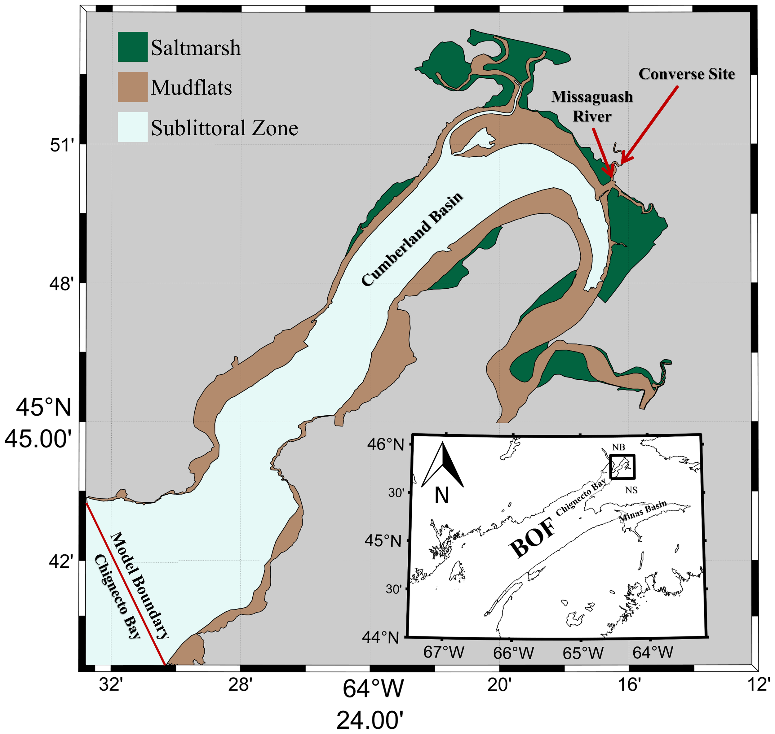
Map of the Cumberland Basin, part of Chignecto Bay in the upper Bay of Fundy (see inset), indicating the Delft3D-FM model water level boundary and the location of the Converse Managed Realignment site on the Missaguash River. Colors denote bottom type regions.
There are several stages of development after tidally driven seawater is allowed to flow into an area previously protected by a dyke (Virgin et al., 2020; Xu et al., 2022). In the ‘preparation stage’, terrestrial vegetation is exposed to salt water and high concentrations of suspended sediment that accumulates and drives high mortality of these plants. In accordance with Xu et al. (2022), the ‘encroachment stage’, is defined by colonization and spreading of salt marsh vegetation and is dependent on site conditions. The ‘adjustment stage’ has continuous vegetation cover across the area and sediment accretion enables the marsh platform to vertically adjust to changes in relative sea-level rise (SLR), provided adequate sediment supply is maintained. For MR to succeed and a salt marsh to re-establish, there must be interactions between sediments, tidal flow, and vegetation (Allen, 2000; Friedrichs and Perry, 2001). It has been found that the success of MR projects is driven by sediment availability (Ganju, 2019) and MRs are considered most effective in locations where there is abundant sediment supply (Liu et al., 2021). Further, van Proosdij et al. (2023) found that tidal wetland restoration at estuary heads can gain from the substantial ecological disturbance created by rapid sediment accretion, which generates a productive substrate with minimal competition from existing vegetation. The BOF is a very sediment-rich coastal environment with average suspended sediment concentrations (SSC) of up to 8 mg·L-1 in the lower bay (Swift et al., 1969) but increasing in the upper reaches up to 200 mg·L-1 in Minas Basin and up to extremely high levels of 3,000 mg·L-1 in Chignecto Bay (Amos and Tee, 1989). Suspended sediment concentrations in tidal rivers of the upper BOF may exceed 40,000 mg·L-1 with ephemeral fluid mud layers (van Proosdij et al., 2023).
Numerical models have previously been used to understand the sediment dynamics in coastal environments. Li et al. (2015) coupled wave and current models with observed grain size in a sediment transport model to predict the seabed shear stresses, sediment mobility, and sediment transport patterns for the entire BOF. Mulligan et al. (2019) used Delft3D coupled with SWAN to simulate the broad-scale tidal circulation, surface waves, and sediment transport to compare seasonal trends in SSC within Minas Basin. Also in Minas Basin, Ashall et al. (2016a) modelled the impacts of tidal energy extraction on the SSC using the Delft3D model and simulated a range of SSC from 2–200 mg·L-1. In recent years as MR has become more frequently adopted on coasts around the world, numerical models have been used to understand the hydrodynamic effects of MR on different coastal systems (Pontee, 2015; Bennett et al., 2020; Kiesel et al., 2020). Spearman (2011) developed a model to predict the evolution of a MR site under the action of tides and waves and sediment supply, building on the hybrid modelling approach that combines process-based and simplified (or empirical) predictive methods. Xu et al. (2022) used a coupled 3-dimensional vegetation-hydrodynamic-morphological modeling system to understand the idealized evolution of a reclaimed salt marsh establishment. There have been few studies that have applied numerical models to help understand the sediment dynamics and geomorphological processes at MR sites in hypertidal environments.
The objective of the present study is to apply a high-resolution numerical model to simulate the sediment transport rates and morphodynamics at a MR site that is in the preparation stage of adjustment. The model results are validated using field observations of water levels, currents, SSC and deposition in a tidal channel, in the dyke breach and over the intermittently flooded land surface behind the dyke. The model results provide insight to the drivers of sedimentary accretion and salt marsh development in the preparation stage of morphological change.
Study site and observations
Converse breach site
The MR site is the Converse breach which is located along the Missaguash River, shown in Figure 2, a tidal river situated in a complex system of bogs, rivers, lakes, and marshes on the north shore of the Cumberland Basin. The Cumberland Basin is part of the upper BOF and the Missaguash River forms the provincial border between Nova Scotia (NS) and New Brunswick (NB). The basin has an area of 121 km2 with a spring tidal prism of 0.90 km3 (Amos and Asprey, 1979) with an intertidal zone of approximately 83 km2 that is predominated by muddy sediments (Amos et al., 1991). Toward the ocean, the Cumberland Basin is connected to the larger Chignecto Bay as shown in Figure 1. van Proosdij et al. (1999) found that the SSC in a nearby salt marsh in the upper Cumberland Basin consisted of 95% coarse silt, with small fractions of clay (2.5%) and sand (1.5%). The salt marshes surrounding Chignecto Bay are a sink for approximately 4 × 10⁵ m3 of sediment annually (Grant, 1980). Amos and Tee (1989) found that the outer parts of the Cumberland Basin have a varying SSC of 50–170 mg·L-1 whereas in the inner parts of the basin the SSC varied between 210–3000 mg·L-1.
Figure 2
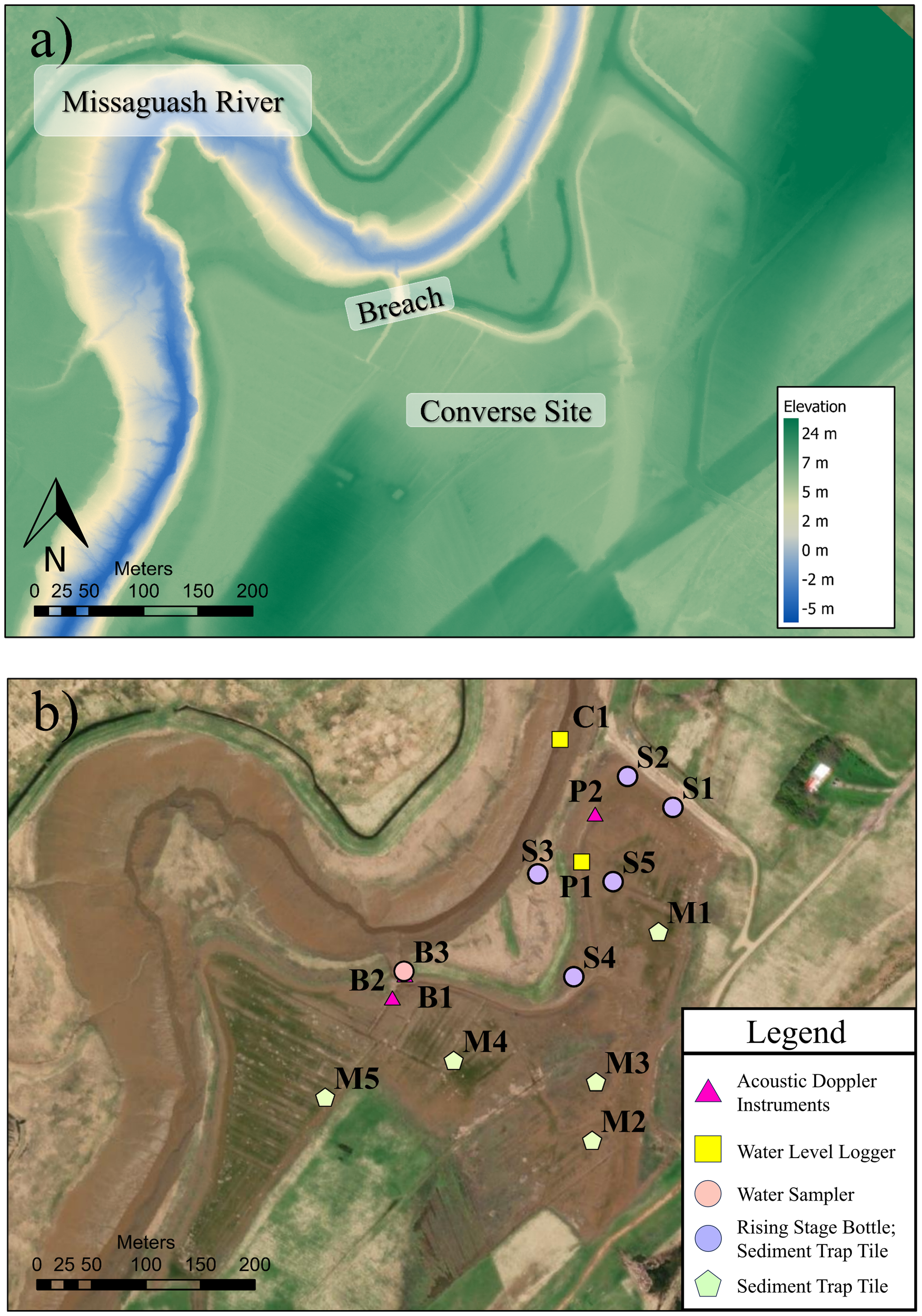
Maps of the Converse Managed Realignment site: (a) LiDAR observations of the topographic elevation relative to the CGVD2013 vertical datum; and (b) aerial image with locations of observation stations in August, 2020.
The Converse Marsh realignment and salt marsh restoration site has experienced increased loss of foreshore marsh, erosion of the dyke at the mouth of Missaguash River, and maintenance of the dyke in its existing location is not feasible. To inform future climate change adaptation and tidal wetland restoration, the dyke at Converse was breached and the aboiteau flood gate structure was removed in December 2018, allowing for 0.164 km2 of abandoned farmland to be exposed to periodic flooding by tidal saltwater (Bowron et al., 2020). Areas of the dyke were graded to the natural foreshore marsh surface elevation to allow marsh flooding during high spring tides. The topography within the breach site is strongly influenced by the historical landscape (Lewis, 2022): small agricultural ditches cover much of the area and a large borrow pit that was created to provide material for the construction of the new realigned dyke is situated within the site. The study period soon after breaching corresponds to the first ‘preparation’ phase, according to the classification defined by Xu et al. (2022), dominated by sediment accumulation in the absence of vegetation.
Field observations
In August 2020, a suite of instruments was deployed in the breach, channels and intertidal areas shown in Figure 2. In the breach at site B1, a 1 MHz Nortek Aquadopp Acoustic Doppler Current Profiler (ADCP) was deployed, sampling at a rate of 16Hz using 30 vertical bins at 0.2m spacing with a total range of 6.2m from the head of the sensor. In close proximity to the ADCP at B1 is an ISCO automated water sampler at site B3. This pumps 500ml water samples at 15-minute intervals with the nozzle located 0.10m from the bed, and observations from B1 and B3 are shown in Figure 3. Within the channels, two Nortek acoustic Doppler velocimeters (ADV) were deployed at sites B2 and P2 and these sampled at a rate of 16Hz, with 4800 samples per burst (5min) every 600 s (10min). Two HOBO water level loggers were installed at sites C1 and P1 to record the water levels every 5 minutes over the course of 4 months.
Figure 3
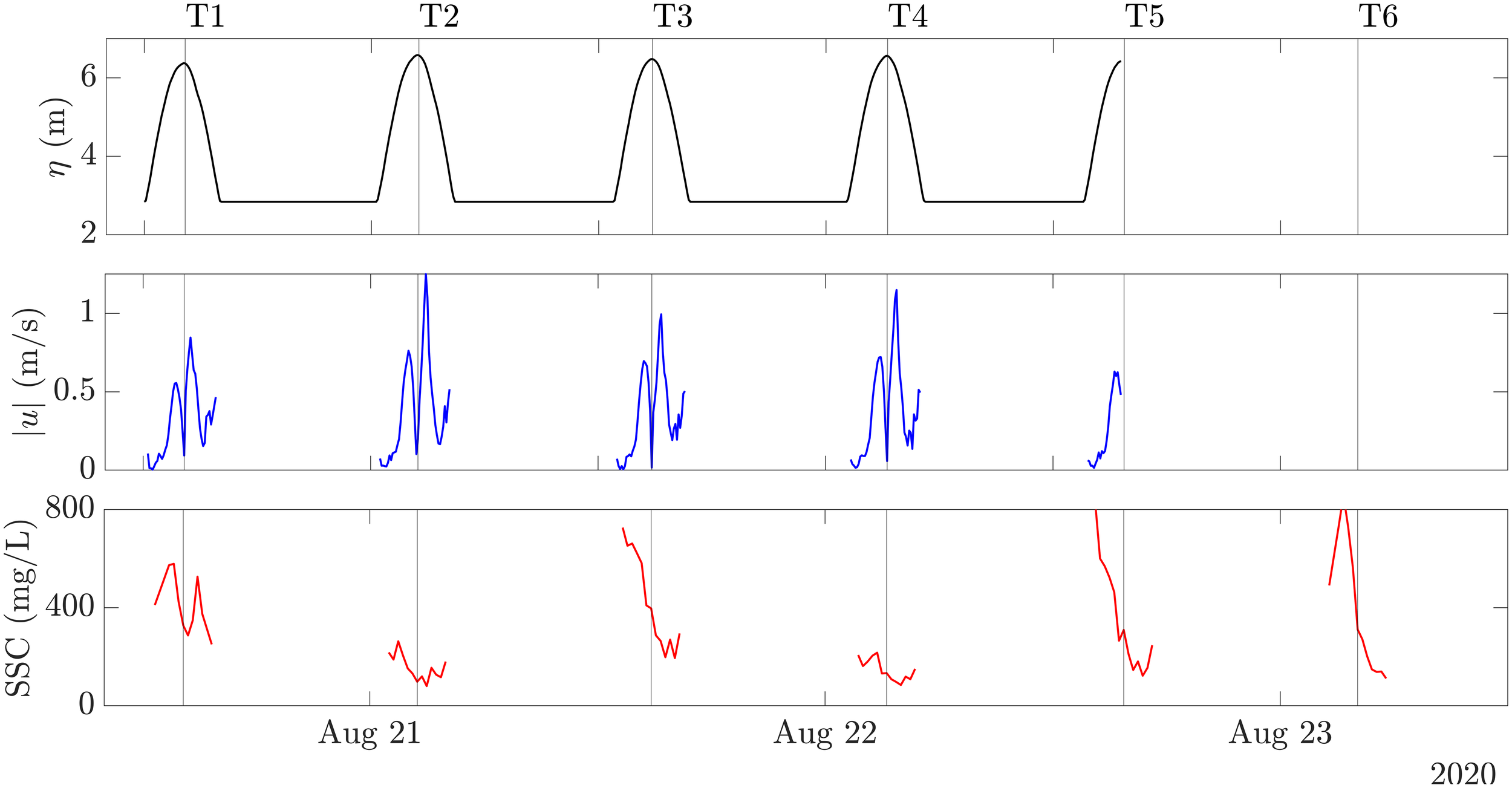
Observations of the water level at B1 (top), current speed at B1 (middle) and suspended sediment concentration (bottom) at B3 measured in the dyke breach channel over 6 tidal cycles in August, 2020. The horizontal lines indicate the high tide time as listed in Table 2.
Dispersed across the area at sites S1 to S5 were 5 Rising Stage Bottles (RSB) to measure SSC; these RSBs consist of a 500ml Nalgene bottle and a rubber bottle stopper with 2 tubes coming out of the top of the bottle to let water in and to let air out, thus, to only collect water entering the site on the rising tide (Graczyk et al., 2000). These bottles were placed directly on the ground, attached to a stake by a hose clamp, with the intake tubes 0.20m above the bed (Elliott, 2023). The water samples with sediments in suspension were collected with ISCO automated water samplers and RSB. The samples were processed using suction with a measured volume, filtered onto pre-weighed 0.8 μm Millipore filter papers, then dried and reweighed to 1 mg precision (Elliott, 2023). The net weight of the filtered sediment and the water sample volume was used to calculate the SSC of each sample to an accuracy of 1 mg·L-1.
Sediment traps were deployed at the same locations as the RSBs as well as at 5 other locations (sites M1–M5) across the marsh to measure the deposition over each of the tides. These stations had sediment trap tiles measuring 6 inches × 6 inches (approximately 0.15m × 0.15m) that were laid rough-side up to prevent sediment from sliding off the tiles and to better mimic the roughness of the adjacent marsh surface (Elliott, 2023), listed in Table 1. The beginning and end of the six tides from August 20-23, 2020, when the observations were made are listed in Table 2 and illustrated in Figure 3.
Table 1
| Observation station | Dates recorded (2020) | Instrument type(s) | Sampling interval | Observations |
|---|---|---|---|---|
| C1 | Jul 20 – Nov 5 | Water level logger (HOBO) | 300 s | Water level |
| B1 | Aug 20 – 22 (5 Tides) | ADCP (Nortek Aquadopp) | 16 Hz | Water level, Current velocity |
| B2 | Aug 20 – 22 (4 Tides) | ADV (Nortek Vector) | 16 Hz | Water level, Current velocity |
| B3 | Aug 20 – 23 (6 Tides) | ISCO Automated Water Sampler | 300 s | SSC |
| P1 | Jul 20 – Nov 5 | Water level logger (HOBO) | 300 s | Water level |
| P2 | Aug 20 – 22 (4 Tides) | ADV (Nortek Vector) | 16 Hz | Water level, Current velocity |
| S1 – S5 | Aug 20 – 22 (5 Tides) | Rising Stage Bottle (RSB), Sediment Trap Tile | 1 Tide | Initial Flood SSC, Deposition |
| M1 – M5 | Aug 20 – 22 (5 Tides) | Sediment Trap Tile | 1 Tide | Deposition |
Summary of observations.
Table 2
| Tide number | Flood start time (First water enters the channel) | Ebb end time (Last water exits the channel) |
|---|---|---|
| T1 | August 20, 13:30 | August 20, 15:00 |
| T2 | August 21, 01:40 | August 21, 03:20 |
| T3 | August 21, 14:05 | August 21, 16:00 |
| T4 | August 22, 02:30 | August 22, 04:20 |
| T5 | August 22, 14:55 | August 22, 16:45 |
| T6 | August 23, 03:25 | August 23, 05:20 |
Definitions of the time of each tide.
Numerical model
Model description
To simulate the hydrodynamics, sediment dynamics and morphology change within the site the Delft3D Flexible Mesh (FM) model (Version 2023.03) was used. Delft3D-FM is an unstructured-mesh hydrodynamic and morphodynamic model that solves the Reynolds-averaged Navier-Stokes equations for incompressible free-surface flow (Lesser et al., 2004). The Delft3D model has been successfully applied to simulate bed morphology change in intertidal zones (Hu et al., 2018) and wetland areas (Liu et al., 2018). It has also been applied to simulate hydrodynamics in back-barrier channels (Manchia et al., 2023) and sediment patterns in highly engineered estuaries such as San Francisco Bay (Van der Wegen et al., 2017; Achete et al., 2017; Allen et al., 2021).
Model set-up and parameter sensitivity
The model topography and bathymetry were defined by combining recent LiDAR data with multibeam bathymetric data (Shaw et al., 2014). The LiDAR data (Crowell, 2021) has a point density of 10 points per meter and covers the northern region of the Cumberland Basin, extending over all of the Converse site. For input to the numerical model, the bathymetric grid was created using LiDAR data acquired in 2021 after the dyke was breached. The bathymetry was interpolated onto a flexible mesh with characteristic horizontal edge lengths that range from 250m in the Cumberland Basin to 1.0m in the MR site, and the model grid the same as presented in Burns et al. (2025). The vertical datum reference used in the model is the Canadian Geodetic Vertical Datum of 2013 (CGVD2013).
The model was forced at the open boundary (Figure 1) using spatially uniform and temporally varying water level and velocity output during spring tides from a depth-averaged structured-grid Delft3D model of the larger Bay of Fundy (Swatridge et al., 2023). Fluid density of 1030 kg·m-3 for sea water, uniform horizontal eddy viscosity of 1 ×10⁻⁴ m2·s-1, and a drying threshold parameter of 0.1m are prescribed over the entire domain. Following sensitivity analysis for different bottom friction coefficients, a map of spatially varying friction coefficients was input to differentiate between three different bottom types (vegetated areas, intertidal mud, and intertidal sand) with Chézy roughness coefficients of 17.9, 65.0 and 57.0 m1/2·s-1 respectively as described in Burns et al. (2025). Vegetation is assumed to have negligible influence on the morphological development in the site, as the bed was sparsely vegetated during the period within the first initial years following the dyke breach. Delft3D-FM was run for a period of 8 days (August 16-23, 2020) to allow for run-up time before comparing to the field observations, using a time step of 0.5 s to maintain a stable courant condition.
For simulating sediment processes, the model was initialized with a zero concentration of cohesive sediment in the water column, and bed shear stress generated by tidal currents is the only mechanism driving suspension. Based on model parameters for fine-grained mud, the sediment parameters were initially set to default model values which include a settling velocity of ws=0.0001 m·s-1, a critical shear stress threshold for erosion of τcre=2.0 N·m-2, a critical shear stress threshold for deposition of τcrd=0.2 N·m-2, and an erosion rate parameter of e=1·10–4 kg·m-2·s-1. After model runs to test the sensitivity for a range of parameter values by comparing the model results with the field observations, we found that that the model results for SSC were sensitive to ws and τcrd. This result suggests that these fine sediments fall faster and out of suspension to settle on the bed at a higher shear stress compared to sediments with the model default parameter values and this can likely be attributed to flocculation. The optimal results were achieved using ws=0.001 m·s-1, and τcrd=0.5 N·m-2 and the results presented use these sediment parameter values.
Model validation
The modelled water level elevations at C1 and P1 are compared to the HOBO water level measurements in Figure 4. At both locations, good agreement between the model result and observations is quantified by correlation coefficients of R2 = 0.99 at C1 and R2 = 0.98 at P1. Based on the detailed analysis of hydrodynamics explained in Burns et al. (2025), the model is able to accurately predict the water level elevations and currents at many other observation sites in the tidal channel, through the breach, and across the flooded land surface behind the breached dyke.
Figure 4
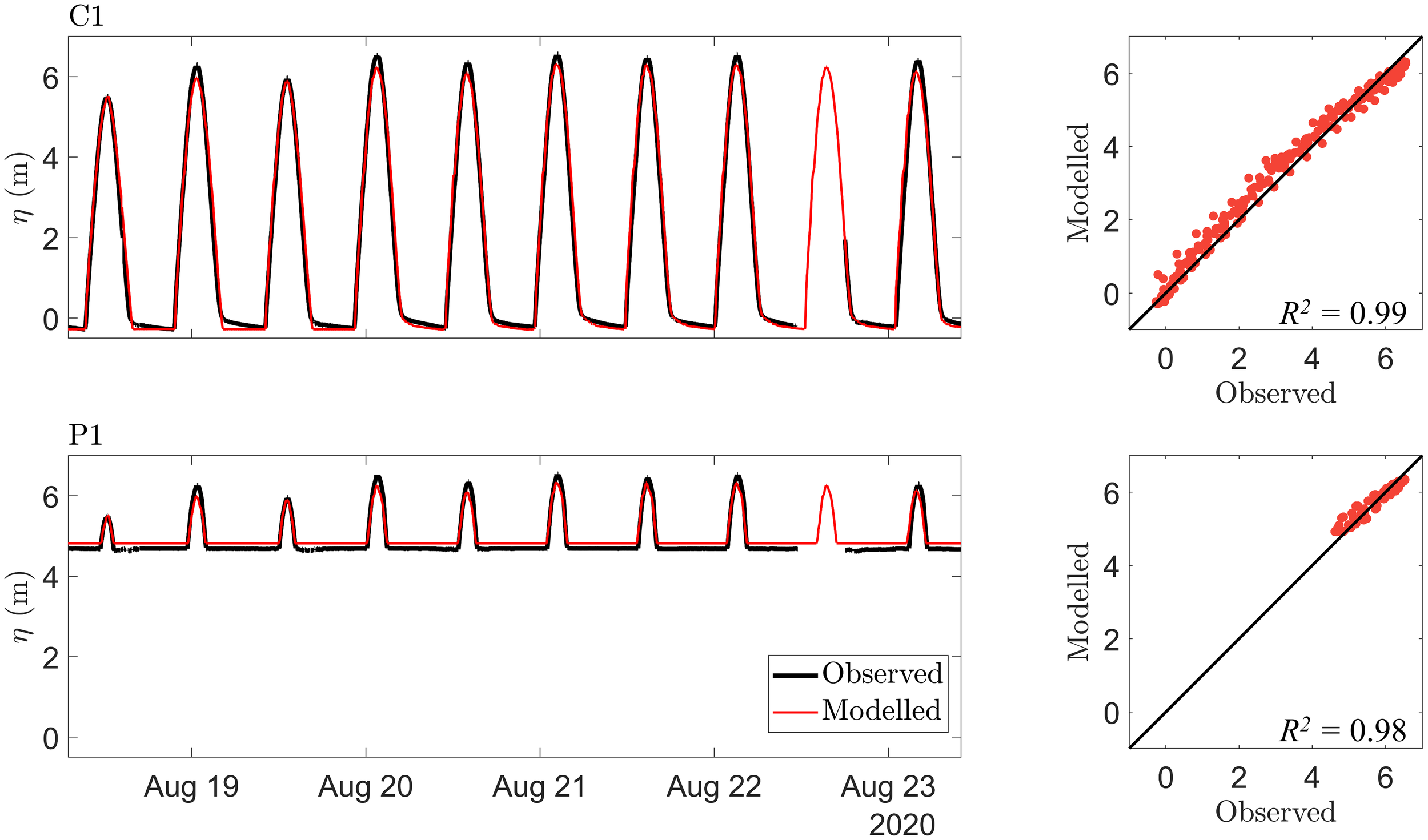
Time series and scatter plots comparing observed and simulated water levels over a selected period of 10 tidal cycles at two locations (C1 and P1), with correlation coefficients indicated in each scatter plot.
The model results for SSC are in general agreement with the temporal evolution of mean SSC indicated by the field observations, but the variability is underestimated in the model due to the depth-averaging. The difference observed within the data can be partially explained through the fact that the water sampler nozzle was located 10cm above the seabed, where the model is depth averaged and takes the SSC of the water closer to the surface into account, lowering the average. The SSC values at B3 are compared to the observations at 15-minute intervals from 90 minutes before and after high tide (negative values are the measurements leading up to high tide, positive values are the measurements past high tide). A total of 6 tidal cycles are summarized in a box and whisker plot in Figure 5. At B3 the ISCO water sampler collected a wider range of values across the 5 tides, and this variability is particularly evident in the inflowing water, where the range of observed values is significantly wider compared to the model predictions. Overall, however, the range of modelled values generally falls within the range of observed data. Additionally, three out of the four days measured had wind speeds around 8–10 m·s-1 from the west, the direction of longest fetch, with very small waves in the channel. Studies in other intertidal areas in the BOF have shown that even small waves over mudflats on rising tides can increase SSC (Mulligan et al., 2019). Since wind and wave effects are not included in the model for this simulation, this omission would likely contribute to lower SSC values in the model output. While the observations show a greater variation in SSC over the 6 tides compared to the modelled (depth averaged) SSC, the modelled SSC values of each time step until -60min relative to high tide (RHT) fall within the range that is observed. At -60 to -90min RHT the model results indicate a very low amount of sediment within the water, where the observations show a more constant SSC (100–400 mg·L-1) after HT (0 RHT). However, both model and observations show a trend of less SSC in water after high tide (water flowing out of the site) than in the water before high tide (water flowing into the site).
Figure 5
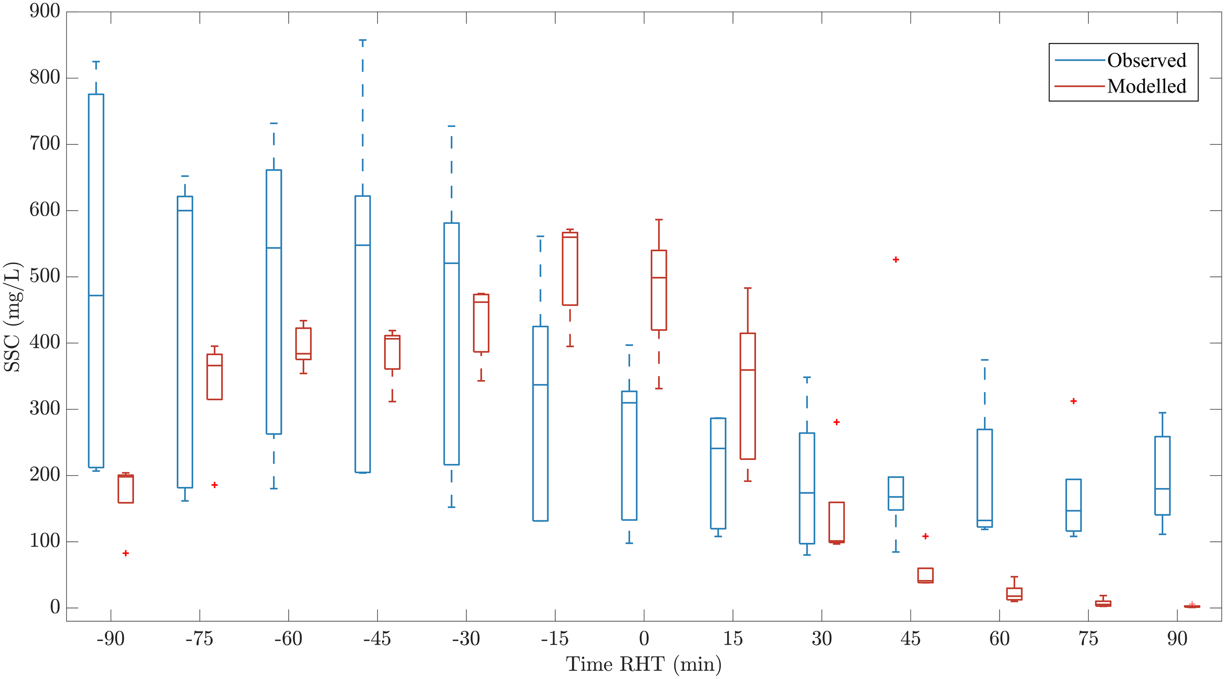
Box and whisker plots of the SSC (mg·L-1) distribution at B3 for observations from the ISCO Automated Water Sampler (blue) and model results (red) averaged over 5 tidal cycles relative to high tide (RHT). The box indicates the interquartile range with the inner line indicating the mean, and the upper and lower ranges indicating the upper (75th) and lower (25th) quartiles respectively; the whiskers denote the upper and lower extremes with + denoting outliers.
The SSC values of the RSB are compared (Figure 6a) to the cumulative SSC over the same duration in the model (Figure 6b), the results are summarized in a box and whisker plot in Figure 6c. The model captures the SSC best at S3 and S4 and the pattern across the site is similar as indicated by the two bar plots (Figures 6a, b). The large difference in measured and modelled SSC values at S4 and S5 could be due to the fact that the RSB only provide a value of the SSC on the incoming flood tide until water depths are about 0.5m above the marsh surface. The bottles were designed for field observations to compare the spatial variability of the availability of sediment. Although there is variability in the difference between model results and field measurements, the modelled SSCs further from the dyke breach (S1 – S3) are in closer agreement with the observations and the simulated cumulative SSC values are within the same order of magnitude as the observations. The observed deposition on the sediment traps across the site are compared to the deposition within the model in Figure 7. The modelled deposition values are also variable but all within the same order of magnitude as the ranges observed across the site (S4, M2, M4, M5) (Figure 7c). Compared to the simulated results, the observations show greater variability in the deposition at each site across the 4 tidal cycles.
Figure 6
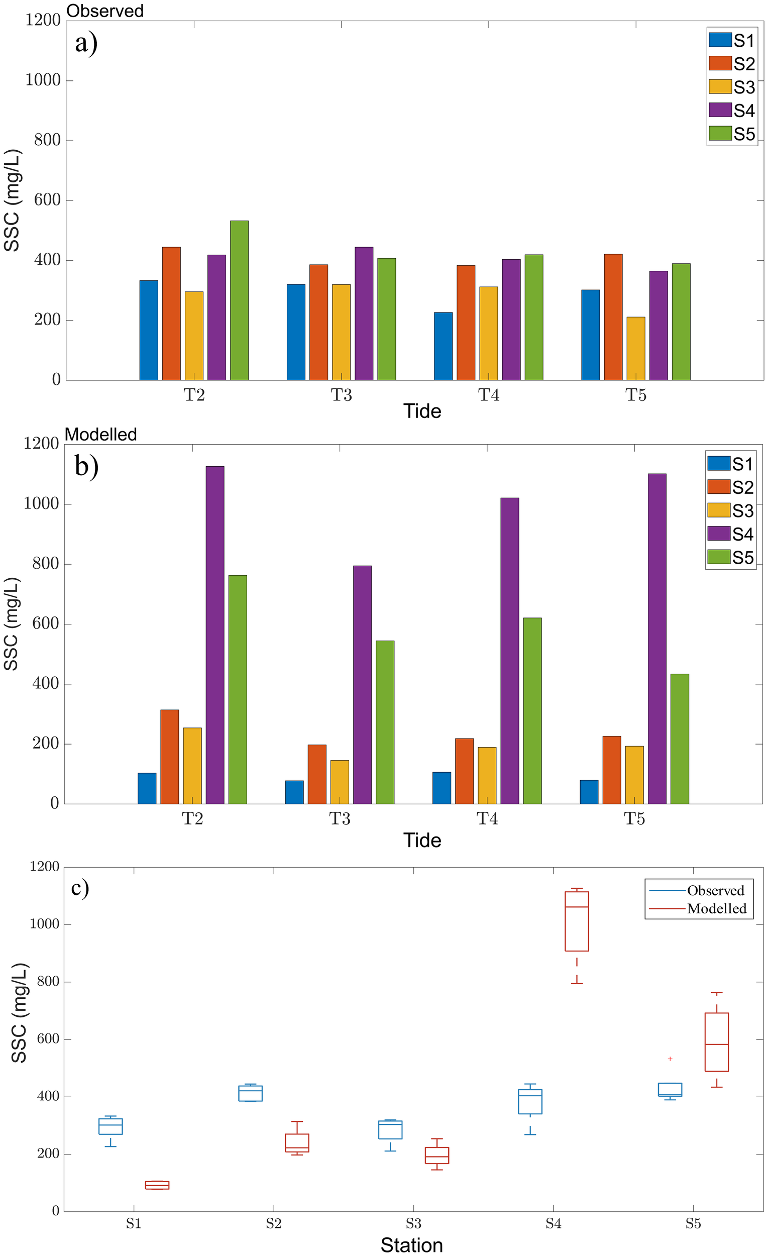
Observations and model results for cumulative SSC: (a) SSC measurements captured by the Rising Stage Bottles (RSB); (b) SSC results from the model; and (c) box and whisker plots of the SSC (mg·L-1) distribution over 5 tidal cycles with observations (blue) and model results (red) across all RSB stations.
Figure 7
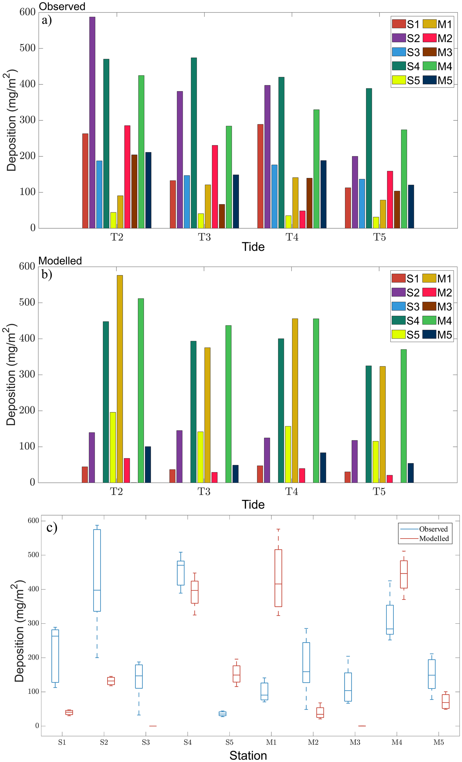
Sediment deposition at the instrument sites, with observed sediment trap measurements compared to the model results: (a) observed deposition; (b) simulated deposition; and (c) box and whisker plots (mg·m-2) indicating the range of deposition over 5 tidal cycles from sediment trap observations (blue) and model.
Results
Spatial distribution of the observed and modelled SSC and deposition shown in Figure 8, overlain on an aerial image. This indicates that the model results for SSC and deposition align most closely with observations near the site’s interior channels, with greater variability observed at points located further away on the marsh platform. The slight underprediction of water levels results in insufficient water coverage in areas farther from the channels, leading to an underestimation of SSC in the model. The evolution of current magnitude and SSC are shown in Figure 9 over one tidal cycle. The flow fields show that topography affects the inflow and outflow at low water as the channels determine the flow propagation and as such the sediment flow throughout the site. The SSC is highest in the tidal channel at around 600 mg·L-1 (at 02:00, Figure 9h) and this highly turbid water flows through the breach into the site, and rushes through the channels and ditches with velocities ranging from 0.5–1.0 m·s-1. As the water flows overtop of the channels and decreases to 0.25 m·s-1 approaching near zero further away from the channels, the sediment drops out of suspension and is deposited across the site. The water with SSC of around 5 mg·L-1 then flows back out to the tidal river.
Figure 8
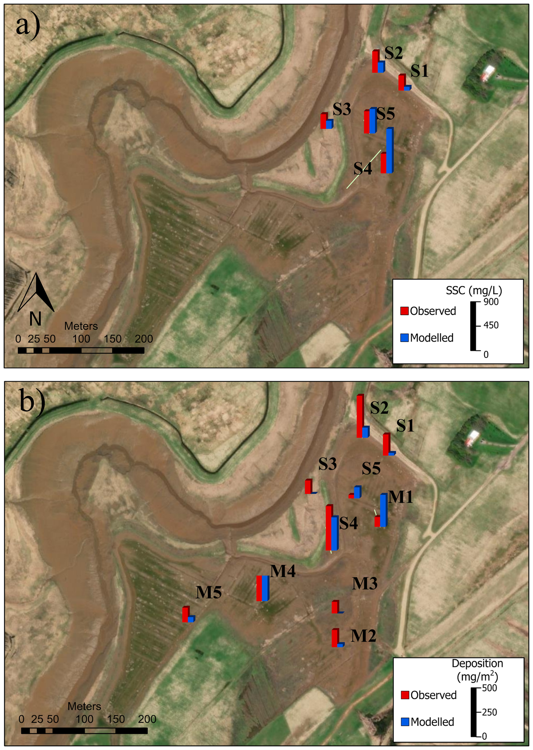
Comparison of observations and model results averaged over 4 tides at each observation station: (a) SSC (mg·L-1) at each RSB station; (b) deposition (mg·m-2) at each sediment trap tile station.
Figure 9
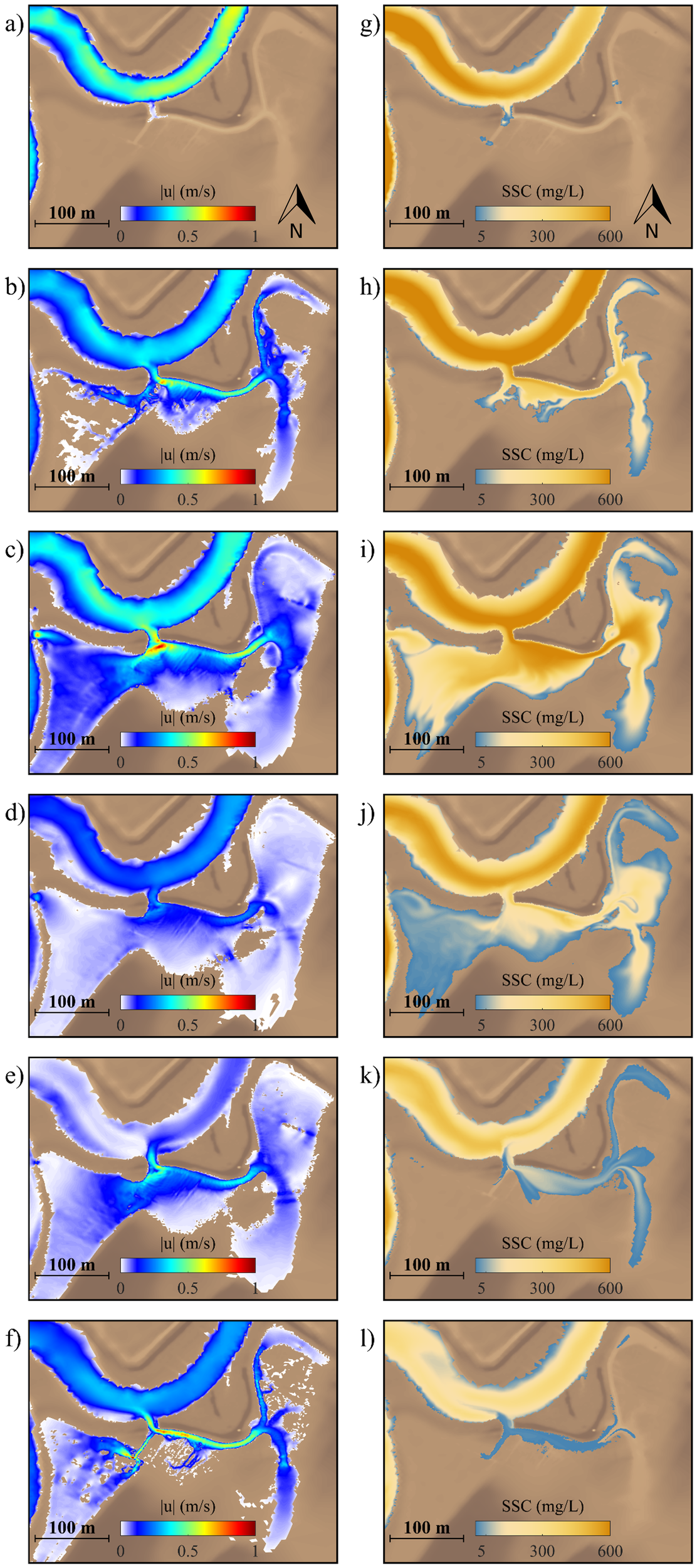
Model results of current magnitude (left) and SSC (right) over a 2.3 hour time period at the peak of one tidal cycle starting on August 21, 01:00 shown in (a) and (g). The maps shown in (b) and (h) are at 02:00 after the channels have filled with water and the following maps follow in 20 minute intervals at times: (c), (i) 02:20; (d), (j) 02:40; (e), (k) 03:00; and (f), (l) 03:20.
Time series of modelled water depth (h) and the depth-averaged current speeds (|u|) are shown in Figure 10 to visualize the velocity magnitudes relative to the SSC and bed level change (Δz) at selected locations. The tidal channel (C1) has the deepest water depth, as well as the fastest current speeds, however the breach (B3) exhibits the highest deposit of sediment. Within the site, the water floods both P2 and M2 with each tide, however, the water depths and duration of flooding at M2 during the first tidal cycle are small, which limits the quantity of suspended sediment reaching this location. Subsequent tides with higher water level elevations are high enough to transport and deposit sediment at M2.
Figure 10
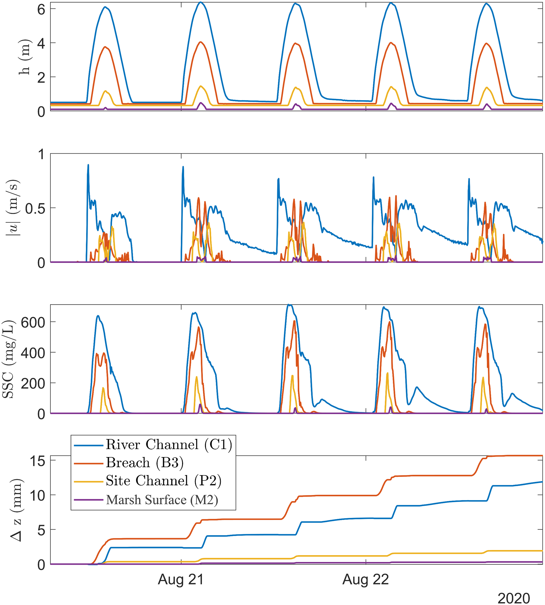
Time series of modelled water levels, depth-averaged current velocities, SSC and bed level change indicating deposition at selected key locations: the tidal river channel outside of the MR site (C1), the breach (B3), the site channel directly behind the dyke (P2) and the field (M2) refers to the new marsh surface. .
The average SSC that flows into the site is depicted in Figure 11a and the flood water carries a decreasing load of SSC as it floods, slows, and deposits sediment across the site. As the water reaches bankfull elevation and flows out across the site, these velocities drop significantly, and the sediment falls out of suspension and is deposited in agreement with other studies (e.g., Leonard et al., 1995; Davidson-Arnott et al., 2002; Poirier et al., 2017). The only region where significant erosion occurs is locally at the corners of the dyke breach channel, and this area has the highest current velocities (Figure 9c). A similar trend in suspended sediment concentration (SSC) is observed in Figure 11b, where sediment deposition is either lower or absent in areas with the highest SSC, and greater in locations where the average SSC ranges between approximately 100–250 mg·L-1. Additionally, areas of high deposition are observed in locations just prior to the point where the average SSC drops below 100 mg·L-1, corresponding with a decrease in current velocities and the attainment of the critical shear stress threshold for deposition. In confined topographic features such as channels and smaller ditches, where current velocities and bed shear stresses are elevated, sediment is transported with the flow. However, as the water moves into unconfined areas the velocity decreases significantly, causing the bed shear stress to fall below the critical threshold for deposition, leading to sediment settling out of suspension.
Figure 11
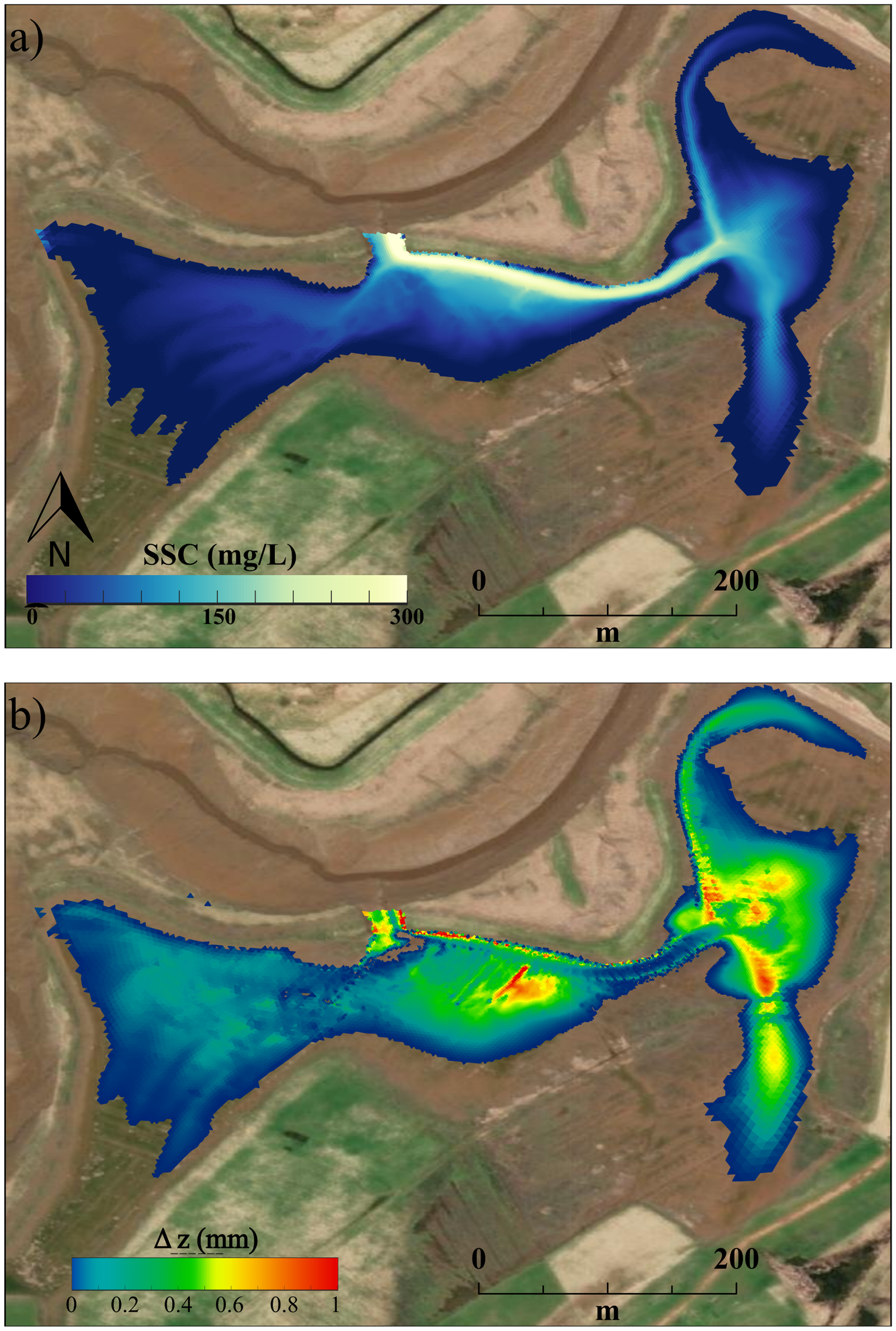
Model results for sediment characteristics averaged over 6 tidal cycles from August 20-23, 2020: (a) average SSC (mg·L-1), ranging from approximately 300 mgL-1 in the channels to around 50 mgL-1 with SSC decreasing the further from the breach; and (b) average deposition, with the spatial mean value of 0.5mm per tidal cycle.
Discussion
Over this tidally flooded platform, the tidal water level elevation is the governing process that drives flow over the surface and carries sediment that ultimately is deposited. A higher tidal elevation in the tidal river outside the breach creates larger velocities that carry higher SSC through the breach and into the ditches, in agreement with previous studies (e.g., Friess et al., 2014; Ashall et al., 2016b). Tidal elevation also increases the inundation time, yielding an important control on the volume of sediment available and increasing the accretion rate. Overall, areas with higher topographic elevation (shallower depth) experience lower accretion rates due to shorter inundation times, aligning with the exponential relationship between inundation time and deposition discussed by Temmerman et al. (2003). As the site of the present study is at relatively high elevation, the channels only begin to fill when the water level reaches approximately 4.7m (relative to the CGVD2013 datum). In contract, at locations further from the breach (e.g., M2), flooding does not begin until the water level reaches 6.0m, and therefore much of the area is not inundated with every single tidal cycle.
Over the entire site the average deposition with each tide is 0.5mm (0.05cm ± 0.04cm), which represents the initial change to the system. For an estimated 80 tides a year (the number of spring tides that exceed the breach elevation) the average deposition would be approximately 4.0 cm·yr-1 ± 3.2 cm·yr-1. This estimated annual accretion rate lies within the ranges of different sites across the upper BOF where accretion was measured. However, this extrapolated model result is likely conservative, and rod surface-elevation table measurements between marker horizons have reported annual accretion rates of 1.0 cm·yr-1 (Bowron et al., 2022) that include the net processes of deposition, erosion and compaction. In comparison to other sites in the upper Bay of Fundy region, similar sediment deposition rates have been estimated at nearby sites (van Proosdij et al., 2006) and rates up to 19 cm·yr-1 (Virgin et al., 2020) and 33 cm·yr-1 (van Proosdij et al., 2023) have been reported. At other MR sites with smaller tides, such as in the Western Scheldt (an estuary in the Netherlands), the accretion rate was measured to be between 1.0 cm·yr-1 (de Vet et al., 2017) and 4.0 cm·yr-1 (de Wilde, 2022). The present site differs from these areas as it is much smaller in area and situated along a comparatively narrow tidal channel. The deposition rate estimated in the present study does not include the effect of ice and ice-rafted sediment, which causes areas of high deposition and scouring along marsh services in the winter and can affect SSC across the Cumberland Basin (Ollerhead et al., 1999; FitzGerald et al., 2020). Using the Representative Concentration Pathway 8.5 high emissions scenario these predictions estimate a maximum of 1.1 cm·yr-1 of sea-level rise as projected by James et al. (2021), which the deposition of sediment would be able to match. Therefore, even if we expect rates of accretion at the marsh site to decrease after the initial build-up, this suggests that the marshes will be sustainable in the face of rising sea levels.
There is a higher discrepancy between the observations and model results in the deposition rate across the site compared to the SSC. One factor that could influence this difference is the flocculation of the cohesive materials, which causes particles to group together and settle much faster than individual particles. There is also a slight underprediction of the peak tidal elevations, as there is a direct link between the duration of flooding at a site and the SSC at a particular location. A slight underprediction in current velocity and water elevation during flooding would lead to reduced bed shear stress and lead to underprediction of SSC. The Delft3D-FM model considers flocculation only through the settling velocity, and in the present study only one sediment type (cohesive mud) is defined. The model does not allow for spatio-temporally varying settling velocities (e.g., resulting from flocculation at higher concentrations, or the effects of turbulence in breaking up flocs), and this is a model limitation. Observations from this site have shown that deposition is not a linear function from distance from channel or elevation gradient (Poirier et al., 2017), with material that flocculates and settles in the tidal channels before it reaches the marsh surface. According to Winterwerp (2001) there are large variations in settling velocities, with higher values around the slack water due to flocculation of sediment under high concentrations. Talke and de Swart (2006) also emphasize the importance of considering a temporally varying settling velocity to properly simulate the behavior of suspended sediment, particularly in high concentrations. Despite the limitations, the model results and field observations together have enabled a detailed picture of tidally-driven sediment transport and geomorphological change of a recently breached dyke and flooded land area to be developed.
Conclusions
Salt marsh restoration through managed realignment of dykes is a potential nature-based solution for enhancing coastal environments and mitigating coastal flood risks. In this study, a recently breached dyke is examined to increase understanding of the sediment processes within the MR site to support the sediment observations. For the first time, the rates of sediment transport and deposition are evaluated in the critical time period immediately following the dyke breach and before the establishment of salt marsh vegetation. The hydrodynamics and sediment transport in the hypertidal Cumberland Basin of the Bay of Fundy are investigated using Delft3D-FM, using the flexible mesh to focus on the MR site. Field observations from 6 tidal cycles in August 2020 are compared to the model results. The tidal water levels and the intertidal topography are found to govern the sediment deposition as the water is directed through the site channels and only floods a greater area of the site for higher water level elevations. High current velocities in the channels quickly decrease after exceeding the bankfull state, and the sediment drops out of suspension as the current velocities reduce. The model results highlight the complexity and difficulty in simulating cohesive sediment processes over small scales, especially at sites with large tidal ranges and high sediment loads. However, the model results clearly indicate that the water depth on the marsh platform and duration of flooding exert significant control on the quantities of sediment that are transported to, and deposited on, the marsh restoration site. Although the sediment dynamics are complex, the results show that the model captures the order-of-magnitude changes in sediment properties over time (within, and between tidal cycles) and trends in spatial variability (e.g., distance from the breach source). The interplay between hydrodynamics and sediment dynamics in the model demonstrate the importance of incorporating accurate topographic and bathymetric data.
We demonstrate that the average deposition rate is 4.0 cm·yr-1 ± 3.2 cm·yr-1 at this site, which falls within the same range as other sites in the upper Bay of Fundy and is higher than the rate of relative sea-level rise in this area. This substantial difference suggests promise for MR and marsh restoration as viable nature-based adaptation strategies for enhancing coastal resilience. The field site is in the preparation phase of marsh development and has minimal vegetation and the modelling approach, which does not incorporate parameterization of the vegetation other than spatially varying bottom roughness, yielded results with the same order of magnitude as the observations. As sediment accumulates and salt marsh plants grow in height and density, future work should be focused on investigating the deposition of sediment in later stages after the salt marsh vegetation has established, as well as examining the effects of long-term sea-level rise on deposition and marsh platform accretion. Combined with field observations the detailed model results of suspended sediment transport and morphology change over a short timescale provide a solid foundation to examine future scenarios related to salt marsh development and evolution over long timescales, relevant to the design of nature-based solution for coastal adaptation.
Statements
Data availability statement
The raw data supporting the conclusions of this article will be made available by the authors, without undue reservation.
Author contributions
RB: Formal analysis, Methodology, Software, Validation, Visualization, Writing – original draft. RM: Conceptualization, Data curation, Formal analysis, Funding acquisition, Investigation, Methodology, Project administration, Resources, Software, Supervision, Validation, Visualization, Writing – original draft, Writing – review & editing. ME: Investigation, Methodology, Writing – review & editing. Dv: Investigation, Methodology, Resources, Writing – review & editing. EM: Funding acquisition, Investigation, Project administration, Writing – review & editing.
Funding
The author(s) declare financial support was received for the research and/or publication of this article. This work was funded by the Canadian Safety and Security Program (CSSP) of Defence Research and Development Canada (DRDC) as part of the Nature-Based Infrastructure for Coastal Resilience and Risk Reduction project. Managed dyke realignment was funded by the Department of Fisheries and Oceans Coastal Restoration Fund to DP and T. Bowron (CA No.17-HMNAR-00533). The Nova Scotia Department of Agriculture is thanked for site access and lidar provided by AGRG, and CBWES Inc are thanked for provision of baseline and post restoration monitoring data. ME was funded by NSERC ResNET project to A. Bennett, McGill University. RM also acknowledges funding from Natural Sciences and Engineering Research Council of Canada (NSERC) Discovery Grant program (RGPIN-2024-04097) and the Department of National Defence (DND) Supplement (DGDND-2024-04097).
Acknowledgments
We would like to thank the Intertidal Sediment Transport Research Unit at Saint Mary’s University, particularly Emma Poirier for collection of field observations, and Laura Swatridge and Delaney Benoit at Queen’s for assistance with the numerical model.
Conflict of interest
The authors declare that the research was conducted in the absence of any commercial or financial relationships that could be construed as a potential conflict of interest.
Generative AI statement
The author(s) declare that no Generative AI was used in the creation of this manuscript.
Any alternative text (alt text) provided alongside figures in this article has been generated by Frontiers with the support of artificial intelligence and reasonable efforts have been made to ensure accuracy, including review by the authors wherever possible. If you identify any issues, please contact us.
Publisher’s note
All claims expressed in this article are solely those of the authors and do not necessarily represent those of their affiliated organizations, or those of the publisher, the editors and the reviewers. Any product that may be evaluated in this article, or claim that may be made by its manufacturer, is not guaranteed or endorsed by the publisher.
References
1
Achete F. van der Wegen M. Roelvink J. A. Jaffe B. (2017). How can climate change and engineered water conveyance affect sediment dynamics in the San Francisco Bay-Delta system? Climatic Change142, 375–389. doi: 10.1007/s10584-017-1954-8
2
Allen J. R. L. (2000). Morphodynamics of Holocene salt marshes: A review sketch from the Atlantic and Southern North Sea coasts of Europe. Quaternary Sci. Rev.19, 1155–1231. doi: 10.1016/S0277-3791(99)00034-7
3
Allen R. M. Lacy J. R. Stevens A. W. (2021). Cohesive sediment modeling in a shallow estuary: model and environmental implications of sediment parameter variation. J. Geophysical Research: Oceans126, e2021JC017219. doi: 10.1029/2021JC017219
4
Amos C. Asprey K. W. (1979). Geophysical and sedimentary studies in the Chignecto Bay system, Bay of Fundy – A Progress Report. Curr. Res. Part B Geological Survey Canada, 245–252. doi: 10.4095/105433
5
Amos C. L. Tee K. T. (1989). Suspended sediment transport processes in Cumberland Basin, Bay of Fundy. J. Geophysical Research: Oceans94, 14407–14417. doi: 10.1029/JC094iC10p14407
6
Amos C. Tee K. T. Zaitlin B. (1991). The post-glacial evolution of Chignecto Bay, Bay of Fundy, and its modern Environment of deposition. Mem. Can Soc Petrol. Geol.16, 59–89.
7
Ashall L. M. Mulligan R. P. Law B. A. (2016b). Variability in suspended sediment concentration in the Minas Basin, Bay of Fundy, and implications for changes due to tidal power extraction. Coast. Eng.107, 102–115. doi: 10.1016/j.coastaleng.2015.10.003
8
Ashall L. M. Mulligan R. P. van Proosdij D. Poirier E. (2016a). Application and validation of a three-dimensional hydrodynamic model of a macrotidal salt marsh. Coast. Eng.114, 35–46. doi: 10.1016/j.coastaleng.2016.04.005
9
Bennett W. G. van Veelen T. J. Fairchild T. P. Griffin J. N. Karunarathna H. (2020). Computational modelling of the impacts of saltmarsh management interventions on hydrodynamics of a small macro-tidal estuary. J. Mar. Sci. Eng.8, 373. doi: 10.3390/jmse8050373
10
Bowron T. M. Graham J. Ellis K. Kickbush J. McFadden C. Poirier E. et al . (2020). Post-restoration monitoring (Year 1) of the Converse Salt Marsh restoration (NS044) – 2019–20 summary Report (Halifax Nova Scotia: Prepared for Department of Fisheries and Oceans & Nova Scotia Department of Agriculture. Publication No. 59).
11
Bleakney J. S (2004). Sods, soil, and spades: The Acadians at Grand Pré and their dykeland legacy (McGill-Queen’s University Press).
12
Bowron T. M. Graham J. Ellis K. Poirier E. Lundholm J. Lewis S. et al . (2022). Post-Restoration Monitoring (Year 3) of the Converse Salt Marsh Restoration (NS044) – 2021–22 Technical Report (Halifax Nova Scotia: Prepared for Department of Fisheries and Oceans & Nova Scotia Department of Agriculture), 142p.
13
Bowron T. Neatt N. van Proosdij D. Lundholm J. Graham J. (2011). Macro-tidal salt marsh ecosystem response to culvert expansion. Restor. Ecol.19, 307–322. doi: 10.1111/j.1526-100X.2009.00602.x
14
Burns R. A. Mulligan R. P. Elliott M. van Proosdij D. Murphy E. (2025). Numerical modelling of the hydrodynamics driven by tidal flooding of the land surface after dyke breaching. Nature-Based Solutions7, 100218. doi: 10.1016/j.nbsj.2025.100218
15
Connor R. F. Chmura G. L. Beecher C. B. (2001). Carbon accumulation in Bay of Fundy salt marshes: Implications for restoration of reclaimed marshes. Global Biogeochemical Cycles15, 943–954. doi: 10.1029/2000GB001346
16
Crowell N. (2021). NSCC-AGRG technical report: 2021 Aulac LiDAR survey. Applied Geomatics Research Group, NSCC, Middleton, NS.
17
Davidson-Arnott R. G. D. Proosdij D. Ollerhead J. Schostak L. (2002). Hydrodynamics and sedimentation in salt marshes: examples from a macrotidal marsh, Bay of Fundy. Geomorphology48, 209–231. doi: 10.1016/S0169-555X(02)00182-4
18
de la Vega-Leinert A. Stoll-Kleemann S. Wegener E. (2018). Managed Realignment (MR) along the Eastern German Baltic Sea: A catalyst for conflict or for a coastal zone management consensus. J. Coast. Res.34, 586–601. doi: 10.2112/JCOASTRES-D-15-00217.1
19
de Vet P. L. M. van Prooijen B. C. Wang Z. B. (2017). The differences in morphological development between the intertidal flats of the Eastern and Western Scheldt. Geomorphology281, 31–42. doi: 10.1016/j.geomorph.2016.12.031
20
de Wilde T. (2022). Hydrodynamic and morphodynamic response of Perkpolder after a managed realignment. MA.Sc. Thesis. Delft, the Netherlands: Delft University of Technology.
21
Dixon M. Morris R. K. A. Scott C. R. Birchenough A. Colclough S. (2008). Managed realignment–lessons from Wallasea, UK. Proc. Institution Civil Engineers - Maritime Eng.161, 61–71. doi: 10.1680/maen.2008.161.2.61
22
Elliott M. (2023). The connections between spatial and temporal variations of hydrodynamic conditions and deposition across a marsh surface restored through managed realignment. M.Sc. Thesis, Halifax, NS: Saint Mary’s University.
23
FitzGerald D. M. Hughes Z. J. Georgiou I. Y. Black S. Novak A. (2020). Enhanced, climate-driven sedimentation on salt marshes. Geophysical Res. Lett.47, e2019GL086737. doi: 10.1029/2019GL086737
24
Friedrichs C. Perry J. (2001). Tidal salt marsh morphodynamics: A synthesis. J. Coast. Res.27, 7–37. Available online at: http://www.jstor.org/stable/25736162.
25
Friess D. A. Möller I. Spencer T. Smith G. M. Thomson A. G. Hill R. A. (2014). Coastal saltmarsh managed realignment drives rapid breach inlet and external creek evolution, Freiston Shore (UK). Geomorphology208, 22–33. doi: 10.1016/j.geomorph.2013.11.010
26
Ganju N. K. (2019). Marshes are the new beaches: integrating sediment transport into restoration planning. Estuaries Coasts42, 917–926. doi: 10.1007/s12237-019-00531-3
27
Garbutt R. A. Reading C. J. Wolters M. Gray A. J. Rothery P. (2006). Monitoring the development of intertidal habitats on former agricultural land after the managed realignment of coastal defences at Tollesbury, Essex, UK. Mar. pollut. Bull.53, 155–164. doi: 10.1016/j.marpolbul.2005.09.015
28
Garrett C. (1972). Tidal resonance in the Bay of Fundy and gulf of Maine. Nature238, 441–443. doi: 10.1038/238441a0
29
Gedan K. B. Kirwan M. L. Wolanski E. Barbier E. B. Silliman B. R. (2011). The present and future role of coastal wetland vegetation in protecting shorelines: Answering recent challenges to the paradigm. Climatic Change106, 7–29. doi: 10.1007/s10584-010-0003-7
30
Graczyk D. J. Robertson D. M. Rose W. J. Steur J. J. (2000). Comparison of water-quality samples collected by siphon samplers and automatic samplers in Wisconsin. USGS Fact Sheet 067-00, July, 0–3. doi: 10.3133/fs06700
31
Grant D. R. (1980). Quaternary sea-level changes in Atlantic Canada as an indication of crustal delevelling. Earth Rheology Isostasy Eustasy, 201–214.
32
Hu K. Chen Q. Wang H. Hartig E. K. Orton P. M. (2018). Numerical modeling of salt marsh morphological change induced by Hurricane Sandy. Coast. Eng.132, 63–81. doi: 10.1016/j.coastaleng.2017.11.001
33
James T. S. Robin C. Henton J. A. Craymer M. (2021). Relative sea-level projections for Canada based on the IPCC Fifth Assessment Report and the NAD83v70VG national crustal velocity model. Geological Survey Canada, 8764. doi: 10.4095/327878
34
Kiesel J. Schuerch M. Christie E. K. Möller I. Spencer T. Vafeidis A. T. (2020). Effective design of managed realignment schemes can reduce coastal flood risks. Estuarine Coast. Shelf Sci.242, 106844. doi: 10.1016/j.ecss.2020.106844
35
Leonard L. A. Hine A. C. Luther M. E. (1995). Surficial sediment transport and deposition processes in a Juncus roemerianus Marsh, west-central Florida. J. Coast. Res.11, 322–336. Available online at: https://journals.flvc.org/jcr/article/view/79546
36
Lesser G. R. Roelvink J. V. van Kester J. T. M. Stelling G. S. (2004). Development and validation of a three-dimensional morphological model. Coastal Engineering51(8–9), 883–915.
37
Lewis S. (2022). Characterizing the evolution of a restoring salt marsh landscape with low altitude aerial imagery and photogrammetric techniques. M.Sc. Thesis, Halifax, Canada: Saint Mary’s University.
38
Li M. Z. Hannah C. G. Perrie W. A. Tang C. C. Prescott R. H. Greenberg D. A. (2015). Modelling seabed shear stress, sediment mobility, and sediment transport in the Bay of Fundy. Can. J. Earth Sci.52, 757–775. doi: 10.1139/cjes-2014-0211
39
Liu K. Chen Q. Hu K. Xu K. Twilley R. R. (2018). Modeling hurricane-induced wetland-bay and bay-shelf sediment fluxes. Coast. Eng.135, 77–90. doi: 10.1016/j.coastaleng.2017.12.014
40
Liu Z. Fagherazzi S. Cui B. (2021). Success of coastal wetlands restoration is driven by sediment availability. Commun. Earth Environ.2, 44. doi: 10.1038/s43247-021-00117-7
41
Manchia C. M. Mulligan R. P. Mallinson D. J. Culver S. J. (2023). Coastal response to the landfall of a hurricane on a series of inlets and narrow back-barrier waterways. Estuaries Coasts46, pp.1690–1708. doi: 10.1007/s12237-023-01242-6
42
Mulligan R. P. Smith P. C. Tao J. Hill P. S. (2019). Wind-wave and tidally driven sediment resuspension in a macrotidal basin. Estuaries Coasts42, 641–654. doi: 10.1007/s12237-018-00511-z
43
Murphy E. Cornett A. van Proosdij D. Mulligan R. P. (Eds.) (2024). Nature-based infrastructure for coastal flood and erosion risk management – a Canadian design guide, Canada, Ottawa: National Research Council. doi: 10.4224/40003325
44
Ollerhead J. van Proosdij D. Davidson-Arnott R. G. D. (1999). “Ice as a mechanism for contributing sediments to the surface of a macro-tidal saltmarsh, Bay of Fundy,” in 1999 Canadian Coastal Conference, Canadian Coastal Science and Engineering Association. 345–358.
45
Poirier E. van Proosdij D. Milligan T. (2017). The effect of source suspended sediment concentration on the sediment dynamics of a macrotidal creek and salt marsh. Continental Shelf Res.148, 130–138. doi: 10.1016/j.csr.2017.08.017
46
Pontee N. I. (2015). Impact of managed realignment design on estuarine water levels. Proc. Institution Civil Engineers - Maritime Eng.168, 48–61. doi: 10.1680/jmaen.13.00016
47
Rupp-Armstrong S. Nicholls R. J. (2007). Coastal and estuarine retreat: A comparison of the application of managed realignment in England and Germany. J. Coast. Res.23, 1418–1430. doi: 10.2112/04-0426.1
48
Shaw J. Todd B. J. Li M. Z. (2014). Geologic insights from multibeam bathymetry and seascape maps of the Bay of Fundy, Canada. Continental Shelf Research83, 53–63.
49
Shepard C. C. Crain C. M. Beck M. W. (2011). The protective role of coastal marshes: a systematic review and meta-analysis. PLoS One6, e27374. doi: 10.1371/journal.pone.0027374
50
Spearman J. (2011). The development of a tool for examining the morphological evolution of managed realignment sites. Continental Shelf Res.31, S199–S210. doi: 10.1016/j.csr.2010.12.003
51
Stronkhorst J. Mulder J. (2014). “Considerations on managed realignment in the Netherlands,” in Managed Realignment: A Viable Long-Term Coastal Management Strategy?, 1st ed(Dordrecht: Springer Netherlands), 61–68.
52
Swatridge L. Mulligan R. P. Boegman L. Shilang S. (2023). “Development and performance of a real-time model of combined tide, surge and waves in the Bay of Fundy,” in Proceedings of the Coastal Sediments 2023, New Orleans LA, USA. 1310–1316.
53
Swift D. J. Pelletier B. R. Lyall A. K. Miller A. J. (1969). Sediments of the Bay of Fundy -a preliminary report. Atlantic Geology5, 95–100. doi: 10.4138/1801
54
Talke S. de Swart H. E. (2006). Hydrodynamics and Morphology in the Ems/Dollard Estuary: Review of Models, Measurements, Scientific Literature, and the Effects of Changing Conditions (IMAU Report R06-01) Civil and Environmental Engineering Faculty Publications and Presentations. 87. Available online at: https://pdxscholar.library.pdx.edu/cengin_fac/87.
55
Temmerman S. Govers G. Wartel S. Meire P. (2003). Spatial and temporal factors controlling short-term sedimentation in a salt and freshwater tidal marsh, scheldt estuary, Belgium, SW Netherlands. Earth Surface Processes Landforms28, 739–755. doi: 10.1002/esp.495
56
van der Wegen M. Jaffe B. Foxgrover A. Roelvink D. (2017). Mudflat morphodynamics and the impact of sea level rise in South San Francisco Bay. Estuaries Coasts40, 37–49. doi: 10.1007/s12237-016-0129-6
57
van Proosdij D. Davidson-Arnott R. G. Ollerhead J. (2006). Controls on spatial patterns of sediment deposition across a macro-tidal salt marsh surface over single tidal cycles. Estuarine Coast. Shelf Sci.69, 64–86. doi: 10.1016/j.ecss.2006.04.022
58
van Proosdij D. Graham J. Lemieux B. Bowron T. Poirier E. Kickbush J. et al . (2023). High sedimentation rates lead to rapid vegetation recovery in tidal brackish wetland restoration. Front. Ecol. Evol.11, 1112284. doi: 10.3389/fevo.2023.1112284
59
van Proosdij D. Lundholm J. Neatt N. Bowron T. Graham J. (2010). Ecological re-engineering of a freshwater impoundment for salt marsh restoration in a hypertidal system. Ecol. Eng.36, 1314–1332. doi: 10.1016/j.ecoleng.2010.06.008
60
van Proosdij D. Ollerhead J. Davidson-Arnott R. G. D. (1999). “Use of optical backscatterance sensors in estimating sediment deposition on a macro-tidal saltmarsh surface,” in Proceedings of the Canadian Coastal Conference, CCSEA. 359–371.
61
Virgin S. D. S. Beck A. D. Boone L. K. Dykstra A. K. Ollerhead J. Barbeau M. A. et al . (2020). A managed realignment in the upper Bay of Fundy: Community dynamics during salt marsh restoration over 8 years in a megatidal, ice-influenced environment. Ecol. Eng.149, 105713. doi: 10.1016/j.ecoleng.2020.105713
62
Winterwerp J. C. (2001). Stratification effects by cohesive and noncohesive sediment. J. Geophysical Research: Oceans106, 22559–22574. doi: 10.1029/2000JC000435
63
Wollenberg J. T. Ollerhead J. Chmura G. L. (2018). Rapid carbon accumulation following managed realignment on the Bay of Fundy. PLoS One13, e0193930. doi: 10.1371/journal.pone.0193930
64
Xu Y. Kalra T. S. Ganju N. K. Fagherazzi S. (2022). Modeling the dynamics of salt marsh development in coastal land reclamation. Geophysical Res. Lett.49, e2021GL095559. doi: 10.1029/2021GL095559
Summary
Keywords
estuaries, salt marshes, sediment transport, coastal morphology, nature-based solutions, Delft3D-FM
Citation
Burns RA, Mulligan RP, Elliott M, van Proosdij D and Murphy E (2025) Sediment dynamics in a dyke breach and across a tidally flooded land surface. Front. Mar. Sci. 12:1626491. doi: 10.3389/fmars.2025.1626491
Received
10 May 2025
Accepted
25 August 2025
Published
08 September 2025
Volume
12 - 2025
Edited by
Jose A. A. Antolínez, Delft University of Technology, Netherlands
Reviewed by
Henry Bokuniewicz, The State University of New York (SUNY), United States
Mireille Escudero, Universitat Politècnica de València, Spain
Updates
Copyright
© 2025 Burns, Mulligan, Elliott, van Proosdij and Murphy.
This is an open-access article distributed under the terms of the Creative Commons Attribution License (CC BY). The use, distribution or reproduction in other forums is permitted, provided the original author(s) and the copyright owner(s) are credited and that the original publication in this journal is cited, in accordance with accepted academic practice. No use, distribution or reproduction is permitted which does not comply with these terms.
*Correspondence: Ryan P. Mulligan, ryan.mulligan@queensu.ca
Disclaimer
All claims expressed in this article are solely those of the authors and do not necessarily represent those of their affiliated organizations, or those of the publisher, the editors and the reviewers. Any product that may be evaluated in this article or claim that may be made by its manufacturer is not guaranteed or endorsed by the publisher.