Abstract
Group discrimination is a critical prerequisite for studying fish population dynamics, implementing effective fisheries management, and evaluating the outcomes of stock enhancement programs. However, research on group differentiation of Oplegnathus fasciatus (Kroyer, 1845), an economically important species in the East China Sea, remains limited across different geographical regions. We conducted a comparative analysis of trace element concentrations, including iron (Fe), manganese (Mn), copper (Cu), zinc (Zn), chromium (Cr), cadmium (Cd), and mercury (Hg), as well as metalloid arsenic (As), in the muscle tissues of three distinct groups of O. fasciatus: the farmed group, the Yangtze River Estuary group, and the Zhongjieshan group. Trace elements were detected using inductively coupled plasma mass spectrometry. Group classification methods such as cluster analysis, stepwise discriminant analysis, and random forest were used to differentiate the groups based on these eight trace elements. Consequently, significant differences were observed in the concentrations of Fe, Cu, Zn, Cr, As, and Hg among the groups (p< 0.05), while differences in Mn and Cr were not statistically significant (p > 0.05). Discriminant analysis showed that cluster analysis effectively differentiated the farmed group from the Zhongjieshan group. Stepwise discriminant analysis achieved an overall accuracy of 85.1%, while the random forest model demonstrated an accuracy of 92.86%. These findings suggest that trace element concentrations could be applied to effectively distinguish among groups of O. fasciatus, with the random forest model outperforming traditional statistical methods to some extent. Our results are relevant to the activities of stock release and fisheries management.
1 Introduction
The economically important rocky warm-temperate fish species Oplegnathus fasciatus (Perciformes, Oplegnathidae, Oplegnathu), commonly known as Japanese parrotfish, mainly inhabits the waters along the coasts of the northwest Pacific, Hawaiian Islands, Mediterranean Sea, and Indian Ocean. It is also distributed in the Yellow and East China Seas in China. This species generally occurs at depths of 15 to 100 m around inshore rocky areas, and its diet consists of small shellfish, crustaceans, and invertebrates. Due to its short migration route, high-density grouping lifestyle, and high economic value, the Chinese government has released millions of cultured juveniles in seawater areas of Zhejiang Zhoushan annually since 2006, and this species has become the main artificial stock release objective species in Zhejiang coastal areas.
In our previous study, we distinguished between natural and cultured groups of O. fasciatus by comparing the otolithic shape and truss characteristics through traditional statistical analysis and neural network methods (Wang et al., 2024a). The neural network approach provided a higher correct identification rate. Meanwhile, we also detected obvious morphological characteristic differences between natural and cultured groups (Wang et al., 2024b). In contrast, Li et al. (2012) found no significant genetic diversity differences between hatchery-released and wild groups in Zhoushan inshore waters when they evaluated amplified fragment length polymorphisms. Additionally, their analysis of molecular variance showed that 96.82% of the genetic variation occurred among individuals within groups, with no significant genetic variation between the two groups (Li et al., 2012). Thus, it is necessary to develop a new method to verify the characteristics that differ between cultured and wild groups in order to assess the effectiveness of artificial stock release. On the other hand, it is also very important to identify the origin of the wild groups for reliable group assessment and fisheries management. Furthermore, it is crucial to develop a method to distinguish their differences among cultured and different wild groups.
The elements essential for living organisms can be classified into categories of trace elements, including copper (Cu), iron (Fe), and zinc (Zn), and ultra-trace elements, including arsenic (As), boron (B), fluorine (F), iodine (I), selenium (Se), cadmium (Cd), chromium (Cr), cobalt (Co), lead (Pb), manganese (Mn), molybdenum (Mo), nickel (Ni), tin (Sn), mercury (Hg), and vanadium (V). While Fe, Mn, Cu, Zn, and Cr play critical physiological roles in aquatic animals, As, Cd and Hg are generally regarded as toxic elements rather than essential elements (Lall and Kaushik, 2021). Trace elements are environmentally ubiquitous, readily dissolved in and transported by water, and readily taken up by aquatic organisms such as marine fishes. Marine fishes assimilate elements through ingestion of particulate material suspended in water, ingestion of food, ion exchange of dissolved elements across lipophilic membranes such as the gills, and adsorption on tissue and membrane surfaces. Excretion of elements occurs via feces, urine, and respiratory membranes. Element profiling has been used to study the provenance of cultured shrimp, clams, sea cucumbers, and fish (Liu et al., 2012; Iguchi et al., 2014; Li et al., 2014, 2015). These studies show that it is possible to use element profiling to identify significant differences in element concentrations in different fish samples and to determine the geographic origins of the fish.
We chose O. fasciatus as our experimental species for several reasons. First, there is a potential market need for this species. In our study area, the price difference between cultured and captured fish is large, so a new laboratory method to distinguish between them is urgently needed. For instance, the market price for wild-caught species such as large yellow croaker (Larimichthys crocea) and salmon (Salmo salar) is significantly higher than that of their farmed counterparts (Nygaard and Roll, 2024). Second, O. fasciatus has limited migration areas. Wang et al. (2022) reported that 85.4% of the total recapturing number was found in< 100 km. Thus, it is possible to compare the trace element concentrations among cultured and different wild groups in a limited spatial range to determine the origin of the fish based on information about limited dietary and environmental conditions.
In this study, we aim to measure the concentrations of Fe, Mn, Cu, Zn, Cr, Cd, As, and Hg in the dorsal muscle of O. fasciatus from three groups: artificial farmed group (AF), the Yangtze River Estuary group (YE), and the Zhongjieshan group (ZJS); analyze the differences in trace element contents using principal component analysis (PCA) and cluster analysis and classify the groups based on stepwise discriminant analysis (SDA) and the random forest model. Given that O. fasciatus is an ecologically and economically important species in Zhejiang coastal waters, this study specifically focuses on regional group differences within this marine area. While our findings are regionally specific, they provide valuable insights into the spatial variation of trace element accumulation in Zhejiang waters and serve as a reference for marine food security, fisheries stock management, and the development of group discrimination methods in similar coastal environments.
2 Materials and methods
2.1 Sample collection and source
In our study, we collected 87 O. fasciatus fish samples: 43 individuals from AF group, 17 individuals from YE group, and 27 individuals from ZJS group. All collected samples were euthanized by gradual cooling and then frozen at –20°C immediately after capture. All procedures were performed in accordance with the “Guidelines for Experimental Animals” of the Ministry of Science and Technology (Beijing, China) and approved by the Institutional Animal Care and Use Committee of Zhejiang Ocean University (ZJOU-AQU-2022-090).
Samples from the AF group were collected at the Xixuan Fisheries Science Island Experimental Aquaculture Station (Figure 1) and measured to an average body length of 103.23 ± 18.86 mm and an average body weight of 47.38 ± 23.64 g. The farming method was high-intensity aquaculture in concrete tanks measuring 5.0 m × 5.0 m × 1.5 m, with lighting provided by daylight lamps at an intensity of 116 lx. Water body exchange rates were maintained at 200–300% per day, with water temperatures and salinity levels kept at 20–22°C and 22–26‰, respectively. In contrast, samples in the YE group had an average body length of 130.41 ± 20.68 mm and an average body weight of 113.00 ± 68.65 g, and were captured using the gillnet fishing boat “Zhepuyu 32128” (44 m long hull, net mesh size of 40 mm) adjacent to the Yangtze River Estuary and coastal waters of northern Zhejiang (Figure 1). Samples from the ZJS group had an average body length of 128.07 ± 13.71 mm and an average body weight of 95.53 ± 37.24 g, and were captured by commercial hook-and-line fishing in the Zhongjieshan Islands sea area (Figure 1). The Zhongjieshan Islands, which are located in the eastern part of the Zhoushan Archipelago, were designated as a national marine protected area and a national marine ranching demonstration zone in 2006 (Liu et al., 2020). Due to the presence of numerous underwater artificial reefs, only commercial hook-and-line fishing is allowed in this area. Considering the potential influence of the reproductive period on trace element accumulation, all samples were collected during the autumn and winter seasons to avoid the spawning period (May–August). This approach aimed to minimize potential biases in the experimental results caused by reproductive activities.
Figure 1
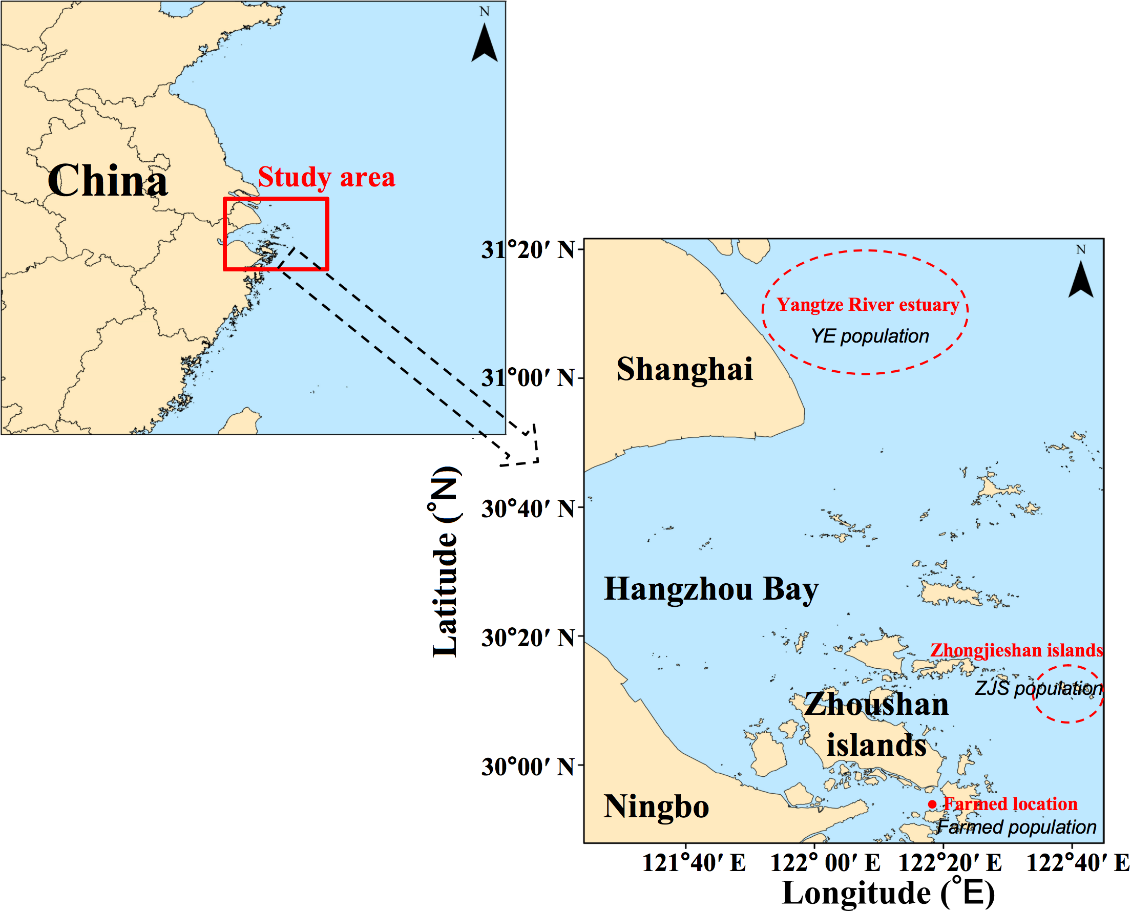
Map showing our study area adjacent to Yangtze River estuary of China. The individual samples were collected from the areas of Yangtze River estuary, Zhongjieshan islands, and a farmed location named as Xixuan Fisheries Science Island Experimental Aquaculture Station.
2.2 Elemental signal analysis
After the frozen samples were thawed, the skinless dorsal muscle was obtained from each sample and weighed to acquire the wet weight. These weight values were recorded for subsequent calculations. The samples were then placed in individual Petri dishes, dried for 48 h using a vacuum freeze dryer (model FD-1-50, Boyikang Instruments Co., Ltd., Beijing, China), and weighed again to obtain the dry weight. Once dried, the samples were ground into a fine powder. For each sample, a 0.03 g portion of the dried sample was used for Hg analysis with a mercury analyzer (DMA-80, Milestone, Sorisole, Italy). Meanwhile, to determine the concentrations of Fe, Mn, Cu, Zn, Cr, Cd, and As in the muscle samples, digestion was performed. Before digestion, all glassware used in the experiments was washed with tap water, purified water, and deionized water and then dried for later use. Deionized water was prepared using a Milli-Q Synergy ultrapure water system (Merck, Rahway, NJ, USA). Due to the complicated composition of fish muscle, the microwave digestion solution was prepared using the HNO3-H2O2-H2O system following the method described by Ni et al. (2020). For each sample, a 0.10 g portion of the dried muscle sample was placed into a polytetrafluoroethylene digestion tube, to which 4 mL of HNO3 (Trace Metal, Thermo Fisher Scientific, Waltham, MA, USA) were added, followed by the addition of 2 mL of H2O2 (superior purity, Sinopharm Chemical Reagent Co., Ltd., Shanghai, China). The mixture was shaken to prevent the sample from adhering to the bottom of the tube. Digestion was performed using an automated microwave digestion system (ETHOSUP, LabTech, Beijing, China), with the system programmed for microwave digestion. After digestion, the cooled digestate was transferred into a 50 mL centrifuge tube and diluted with deionized water to a final volume of 50 mL. The concentrations of elements in the tissue samples were measured using an inductively coupled plasma mass spectrometer (model 7900a, Agilent Technologies, Santa Clara, CA, USA). High-purity argon gas (Ar, 99.999%) was used as the plasma, auxiliary, and nebulizer gas, while high-purity helium gas (He, 99.999%) was used as the collision gas. Quality control of the detection method was performed by simultaneous analysis of the standard reference material for freeze-dried salmon muscle (GBW 10210), which was obtained from the National Research Center for Certified Reference Materials (NRCCRM), Beijing, China. The recovery rates for Hg, Cr, Mn, Fe, Cu, Zn, As, and Cd were 85.9%, 99.9%, 115%, 110.2%, 92.3%, 86.4%, 85%, and 86.6%, respectively, which met the quality control requirements. In our study, vacuum freeze-drying was used.
2.3 Data calculations and statistical analysis
The element concentrations measured in the samples using inductively coupled plasma-mass spectrometry were calculated based on the dry weight of the samples (mg kg–1 dw). To facilitate comparison with other studies, the values were converted to wet weight (mg kg–1 ww) using moisture content as the conversion factor following the methods described by Korkmaz et al. (2019) and LaBine et al. (2021). The calculation formula is as follows (Equations 1–3):
where M represents the moisture content of the muscle sample; W1 is the weight of the muscle sample before drying; W2 is the weight of the muscle sample after drying; R is the conversion factor from dry weight concentration to wet weight concentration; WW is the wet weight concentration of the sample, and DW is the dry weight concentration of the sample.
To evaluate the growth condition of the samples, Fulton’s condition factor (K) was calculated using the relationship between whole body weight (BW, g) and body length (BL, cm) according to previous studies (Milatou and Megalofonou, 2014; Piras et al., 2023) (Eqaution 4):
In addition, statistical analyses for the eight trace elements were conducted using a combination of parametric and multivariate methods. A one-way analysis of variance (ANOVA) was first performed to compare trace element concentrations among the three groups (O. fasciatus from AF, YE, and ZJS groups). When significant differences were detected, Tukey’s honestly significant difference test was applied for post hoc multiple comparisons. Statistical significance was set at p< 0.05 as statistically significant, p< 0.01 as highly significant, p< 0.001 as very highly significant, and p< 0.0001 as extremely significant.
To explore overall variation and clustering patterns in the element profiles, PCA and cluster analysis were performed on the measured element data, followed by SDA to differentiate among the three groups of O. fasciatus. Factors were selected for inclusion in the discriminant function based on the Wilks’ Lambda method, which evaluates each variable’s contribution to group differentiation. A discriminant equation was then established to predict group membership, with accuracy rates determined through cross-validation. All statistical analyses, including PCA, cluster analysis, and SDA, were conducted using SPSS 27.0 software (IBM, Armonk, NY, USA).
In addition to traditional SDA, a random forest-based classification method was employed to analyze the top six indicators identified through PCA. The data were randomly divided into a training set (70%) and a testing set (30%), and the model’s accuracy was evaluated by comparing the observed values with the predicted values. Considering the use of an imbalanced dataset, macro-averaged precision, macro-averaged recall, macro-averaged F1 score, and G-mean were used to assess the performance of the model. The random forest model was implemented using the scikit-learn package in Python 3.8 (https://www.python.org/).
3 Results
3.1 Analysis of trace element contents and their correlation with Fulton’s K index in O. fasciatus from different groups
High significant differences (P< 0.01) in the concentrations of Fe, Cu, Zn, Cd, As, and Hg in the muscle tissues of O. fasciatus samples were detected among the different groups (Figure 2). The ZJS group had significantly higher concentrations of Fe, Cd, and As compared to the other two groups, while the Hg concentration in the AF group was significantly higher than that of two wild groups (Figure 2).
Figure 2
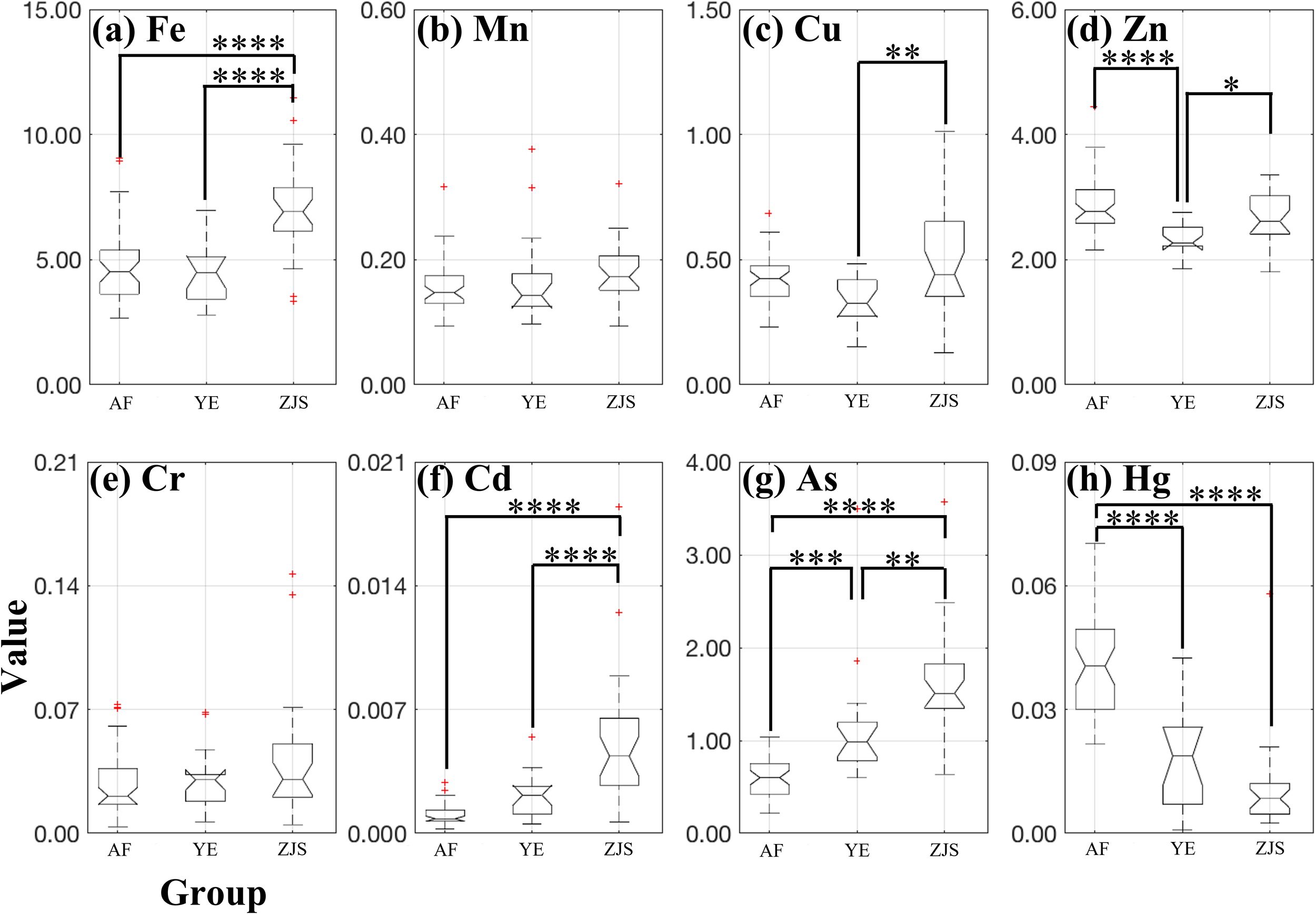
Box plots of trace element content including (a) iron Fe in a value range of 0–15 mg kg-1, (b) manganese Mn in a value range of 0-0.6 mg kg-1, (c) copper Cu in a value range of 0-1.5 mg kg-1, (d) zinc Zn in a value range of 0–6 mg kg-1, (e) chromium Cr in a value range of 0-0.21 mg kg-1, (f) cadmium Cd in a value range of 0-0.021 mg kg-1, (g) arsenic As in a value range of 0–4 mg kg-1, and (h) mercury Hg in a value range of 0-0.09 mg kg-1, in the muscle tissues of three distinct groups of Oplegnathus fasciatus: the farmed group (abbreviated as ‘AF’), the Yangtze River estuary (abbreviated as ‘YE’) group, and the Zhongjieshan (abbreviated as ‘ZJS’) group. The symbols ‘*’ indicates statistically significant (P< 0.05); ‘**’ indicates highly significant (P< 0.01); ‘***’ indicates very highly significant (P< 0.001); ‘****’ indicates extremely significant (P< 0.0001).
The Fulton’s condition index (K) ranged from 3.06 to 5.36 in the AF group, with a mean value of 3.94 ± 0.50. In the YE group, K ranged from 4.22 to 5.39, with a mean of 4.79 ± 0.33, while in the ZJS group, the range was 3.04 to 5.52, with a mean of 4.39 ± 0.49. To examine the relationship between somatic condition and trace element accumulation, Pearson correlation coefficients were calculated between Fulton’s K index and six trace elements (Fe, Cu, Zn, Cd, As, and Hg) that showed significant differences among the different groups (Table 1). The results revealed that Fulton’s K index was negatively correlated with Zn, Hg and Fe across all three groups. In the YE group, K showed a positive correlation with Cu, whereas in the AF and ZJS groups, these correlations were negative but relatively weak. A positive correlation between K and As was observed in the AF group, while negative correlations were noted in the YE and ZJS groups. Among these relationships, significant negative correlations between K and Hg were found in the AF (r = −0.46, p< 0.01) and YE (r = −0.54, p< 0.05) groups (Figure 3).
Table 1
| Component | Initial eigenvalue | Extraction sums of squared loadings | ||||
|---|---|---|---|---|---|---|
| Total | Variance percentage | Cumulative variance percentage | Total | Variance percentage | Cumulative variance percentage | |
| First | 2.45 | 41.64 | 41.64 | 2.50 | 41.64 | 41.64 |
| Second | 1.58 | 26.30 | 67.94 | 1.58 | 26.30 | 67.94 |
| Third | 0.69 | 11.41 | 79.35 | — | — | — |
| Fourth | 0.58 | 9.67 | 89.02 | — | — | — |
| Fifth | 0.36 | 5.94 | 94.96 | — | — | — |
| Sixth | 0.30 | 5.04 | 100.00 | — | — | — |
Total variance explained by principal component analysis, including initial eigenvalues, and extraction sums of the square of the load.
Figure 3
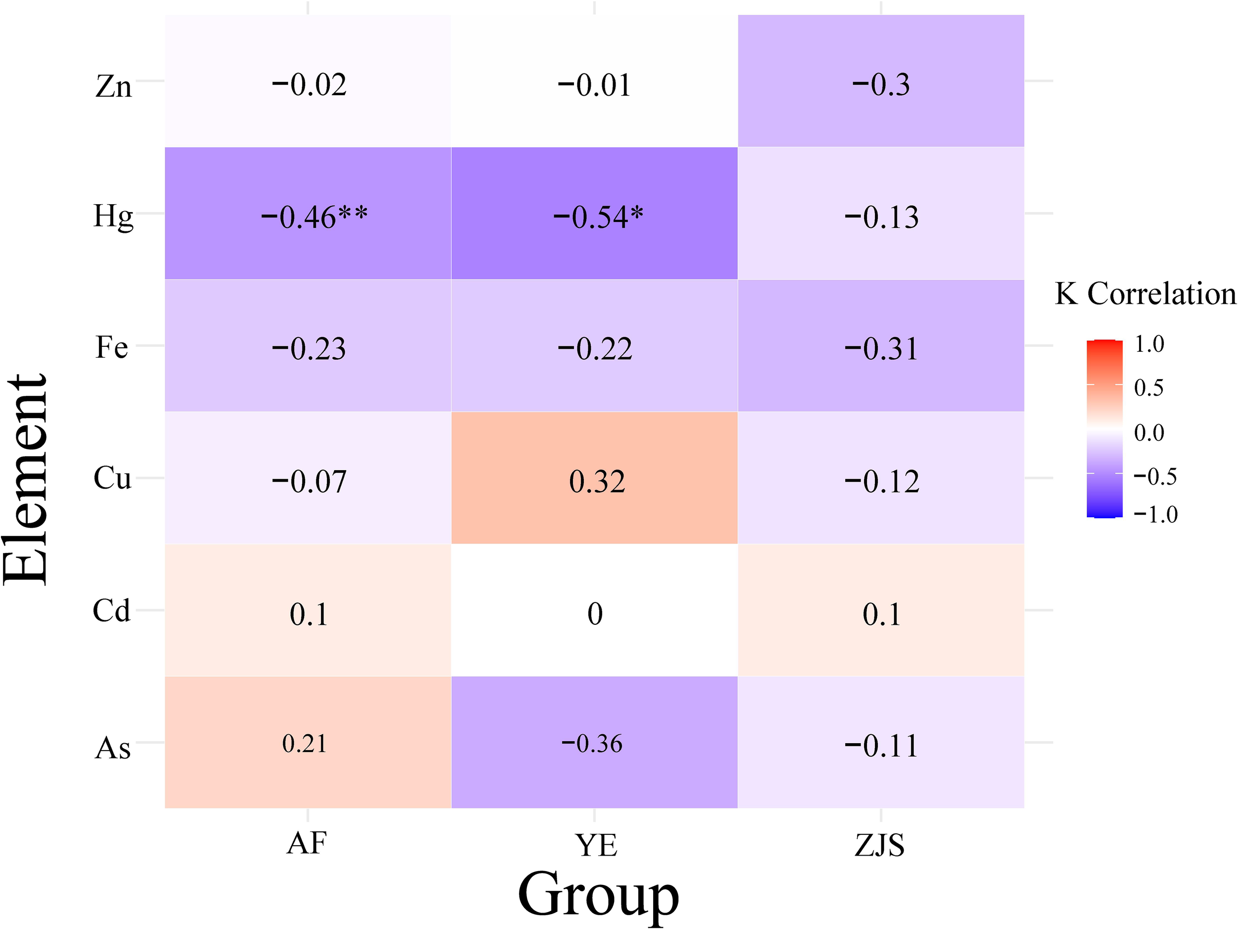
Results of Pearson correlation analysis between Fulton’s condition factor (K) and six trace elements (Fe, Cu, Zn, Cd, As, and Hg) in the muscle tissues of fish from three groups: AF, YE, and ZJS. The right bar shows the correlation closeness between 1.0 represented by red and −1.0 represented by blue. The symbols ‘*’ indicates statistically significant (P< 0.05); ‘**’ indicates highly significant (P< 0.01).
3.2 PCA and cluster analysis of trace element contents
PCA was performed on the six elements (Fe, Cu, Zn, Cd, As, Hg) that showed significant differences among the different groups (Table 1). The variance contribution of the first principal component (PC1) was 41.64%, while the second principal component (PC2) contributed 26.30% and the third principal component contributed 11.41% of the total variance. The cumulative variance contribution of the first three principal components reached 79.35%. Additionally, the eigenvalues of PC1 (2.50) and PC2 (1.58) were both > 1, meeting the standard criterion for selection as principal components. Therefore, PC1 and PC2 were chosen as the primary dimensions for subsequent analysis (Table 1), as they reduce data complexity while preserving the key features and major variability within the dataset.
The cumulative variance contribution of the first two principal components reached 67.94%, indicating that 67.94% of the information originally represented by the six variables can be acquired by these two components. Specifically, PC1 primarily integrated information about Fe, Cd, and As concentrations, and PC2 primarily integrated the information about Zn, Cu, and Hg concentrations (Table 2).
Table 2
| Indicators | Components | |
|---|---|---|
| First | Second | |
| Fe | 0.70 | 0.12 |
| Cu | 0.64 | 0.63 |
| Zn | 0.22 | 0.85 |
| Cd | 0.76 | −0.11 |
| As | 0.77 | −0.33 |
| Hg | −0.61 | 0.57 |
Variance contributions and eigenvector values of the first two principal components of the indicators including Fe, Cu, Zn, Cd, As, and Hg.
PC1 and PC2 were used as the horizontal and vertical axes, respectively, to create the PCA plot (Figure 4). The AF group, YE group, and ZJS group were mainly located in the upper left area, the lower left area, and the right area, respectively. The YE group showed considerable overlap with the other two groups (Figure 4).
Figure 4
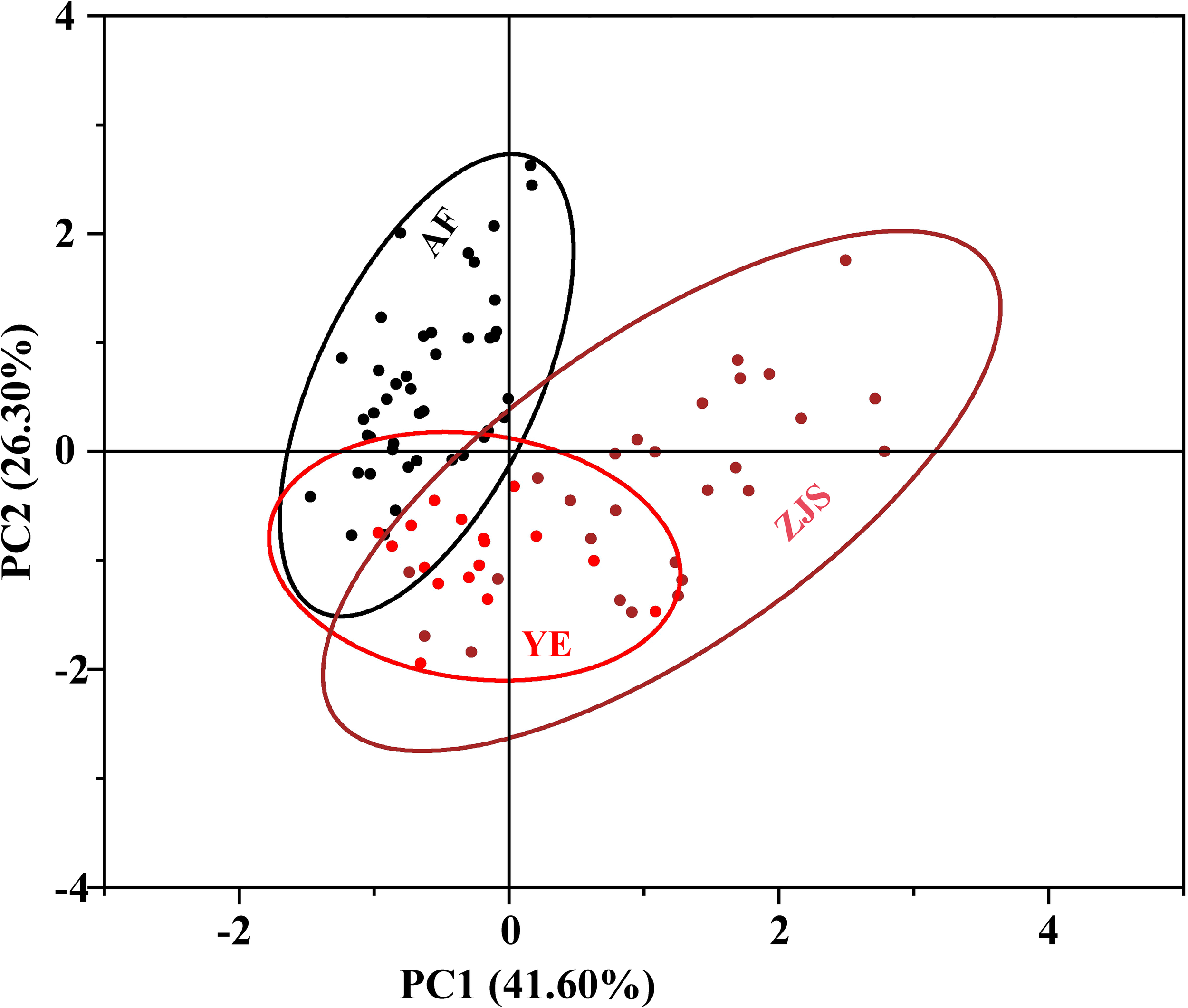
Standardized score plot of the first two principal components (PC1 41.60% against PC2 26.30%) of the fish species Oplegnathus fasciatus individuals number. The colors of black, red, and brown filled dots and solid lines represent the groups of artificial farmed (AF), Yangtze River estuary (YE), Zhongjieshan islands (ZJS), respectively.
To better assess the classification of groups based on trace element indicators, hierarchical cluster analysis was performed using the standardized scores of the first two principal components (Figure 5). Through cutting the dendrogram at a clustering distance of 2.25, the samples were divided into four categories: i) primarily AF samples plus 4 ZJS and 13 YE samples; ii) all AF samples; iii) mainly ZJS samples and 4 YE samples; and iv) 3 ZJS samples. These results suggest that trace element content had potential to distinguish the ZJS group from the other two groups, but it was less effective for the classification between the AF and YE groups.
Figure 5
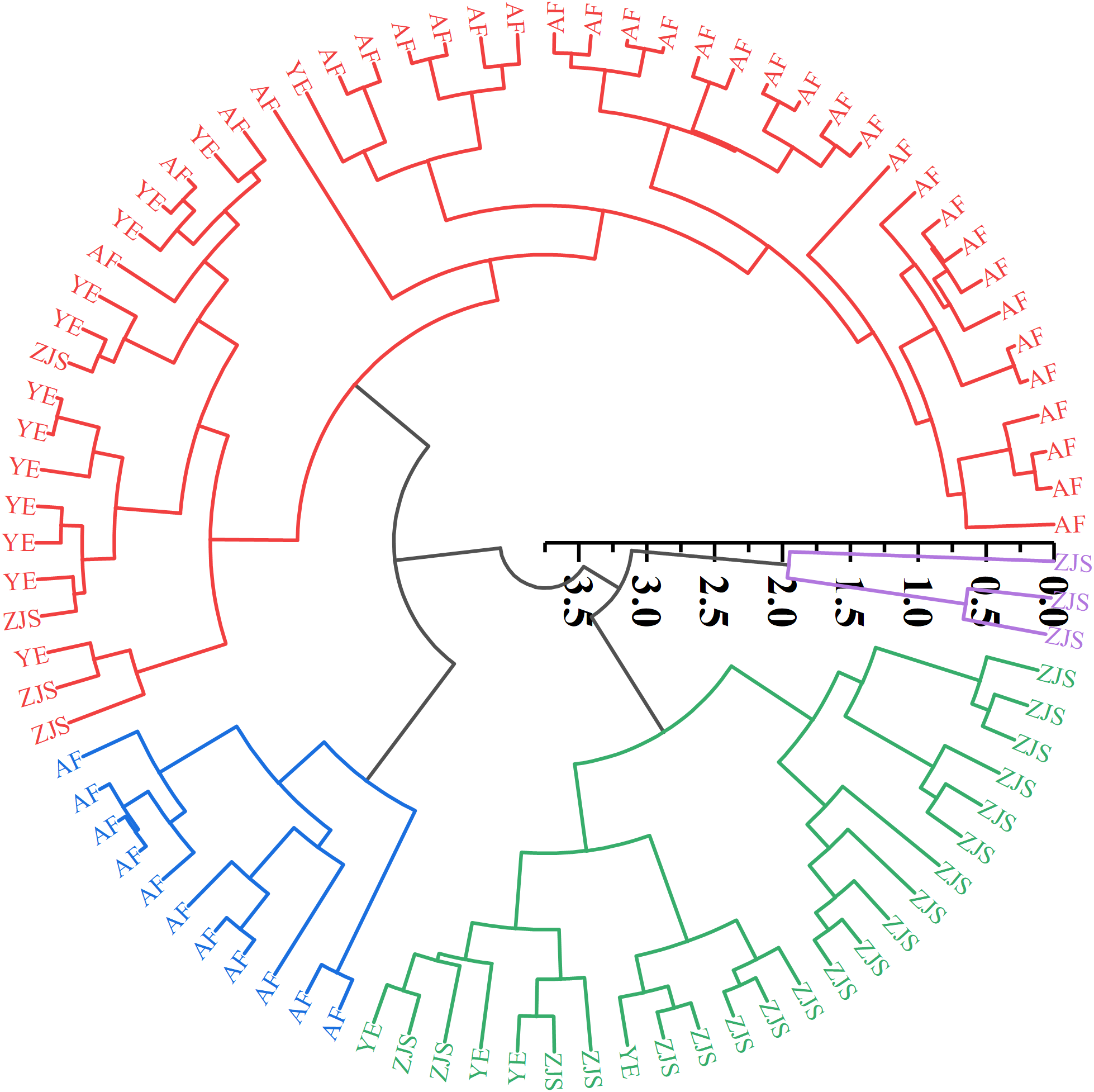
Hierarchical clustering dendrogram of fish species Oplegnathus fasciatus individual samples including the farmed group (abbreviated as ‘AF’), Yangtze River estuary group (abbreviated as ‘YE’), and Zhongjieshan group (abbreviated as ‘ZJS’) according to the first two principal components. The Arabic number indicates the distance among samples according to the calculations of the first two principal components. The colors represent different groups in a clustering distance of 2.25.
3.3 Group classification based the SDA and random forest methods
After performing SDA and using the Wilks’ Lambda method to screen the eight trace element indicators in the muscle of O. fasciatus, five variables were obtained as inputs for the discriminant function: X1 (Fe), X2 (Zn), X3 (Cd), X4 (As), and X5 (Hg) The discriminant functions were established as follows (Equations 5–7):
By substituting the selected five variables into the discriminant function, three function values (Y1, Y2, and Y3) were obtained. The group corresponding to the function with the highest value was considered to be the group to which the sample belonged. The discriminant results (Table 3) indicated that the initial classification accuracies for the AF, YE, and ZJS groups were 88.4%, 88.2%, and 81.5%, respectively, with an overall accuracy of 86.2%. After cross-validation, the classification accuracy for the AF group dropped slightly to 86.0%, while the rates for the other two groups remained unchanged, resulting in an overall accuracy of 85.1%. The classification accuracy for the AF and YE groups exceeded 85.0%, and it was above 80.0% for the ZJS group (Table 3). These results indicated that this linear model effectively differentiated the three groups.
Table 3
| SDA | Actual group | Predicted group | Total | Accuracy (%) | Total accuracy (%) | ||
|---|---|---|---|---|---|---|---|
| AF | YE | ZJS | |||||
| Original | AF | 38 | 5 | 0 | 43 | 88.4 | 86.2 |
| YE | 0 | 15 | 2 | 17 | 88.2 | ||
| ZJS | 1 | 4 | 22 | 27 | 81.5 | ||
| Cross-validation | AF | 37 | 6 | 0 | 43 | 86.0 | 85.1 |
| YE | 0 | 15 | 2 | 17 | 88.2 | ||
| ZJS | 1 | 4 | 22 | 27 | 81.5 | ||
Group classification of Oplegnathus fasciatus for the groups of artificial farmed (‘AF’), Yangtze River estuary (‘YE’), and Zhongjieshan (‘ZJS’) according to stepwise discriminant analysis (SDA).
The random forest model created using 70% of the samples as the training set achieved an overall training accuracy of 100.0%. The trained model was then tested on the remaining samples, and the error rate curve during model testing (Figure 6) showed that when fewer than 20 trees were used, error rates for each group were relatively high and fluctuated significantly. As the number of trees increased, the error rates for each group and the overall error rate gradually decreased. The error rate for the ZJS group stabilized at 25 trees, and the error rates for the AF and YE groups stabilized at 40 trees and 55 trees, respectively. The error rate for the AF group was generally lower than that for the YE and ZJS groups. The test results indicated that the precision values for the AF, YE, and ZJS groups were 1.00, 0.83, and 0.88, respectively; the sensitivity values were 1.00, 0.83, and 0.88, respectively; and the F1-scores were 1.00, 0.83, and 0.88, respectively. The overall accuracy of the model was 92.86%, indicating strong classification performance, particularly for the AF and ZJS groups. Furthermore, the macro-averaged precision, recall, and F1-score all reached 0.903, and the G-mean value of 0.904 further reflects the model’s balanced effectiveness across all three groups.
Figure 6
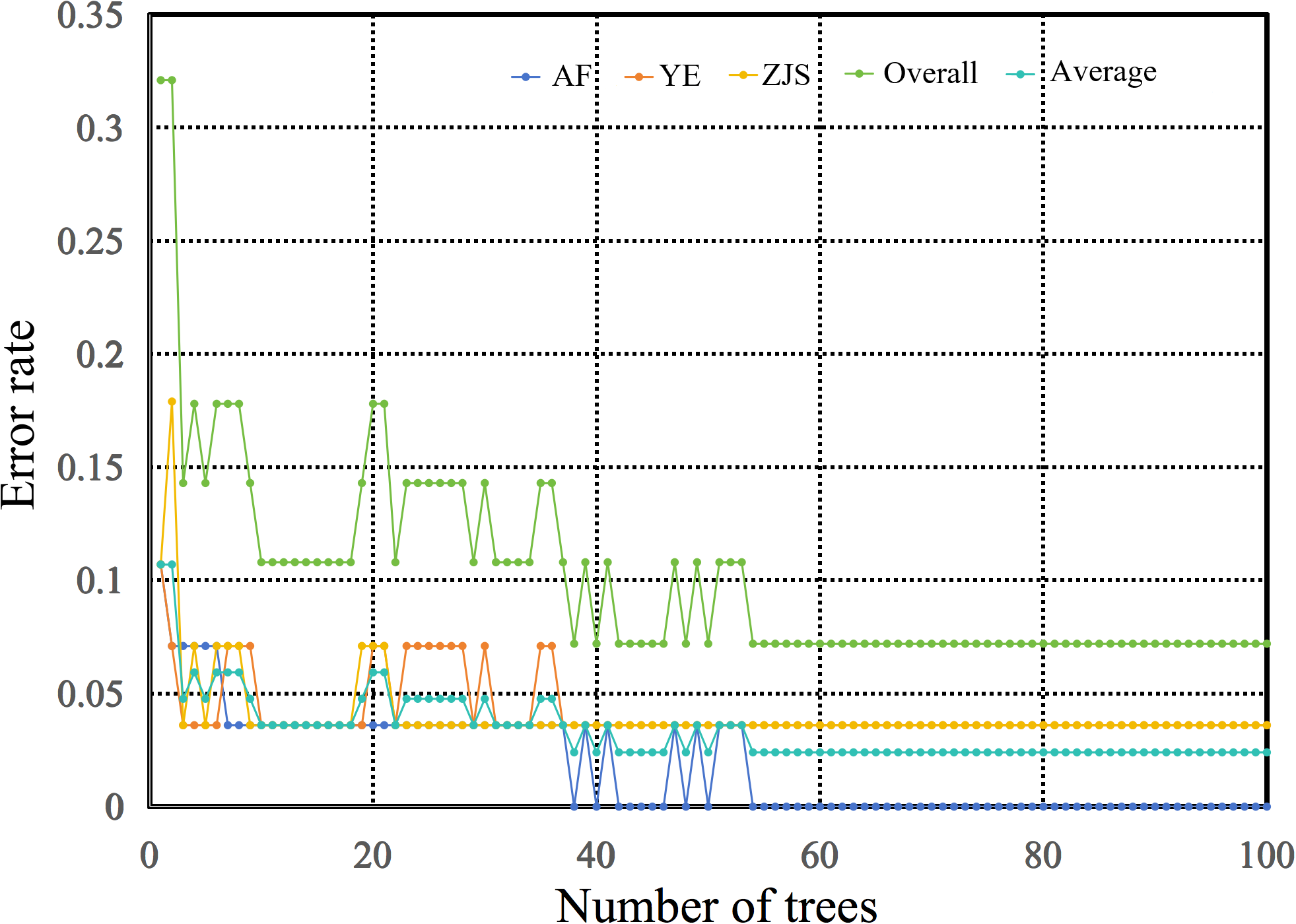
The plot of error rate in a range of 0 to 1 against number of trees to represent error rate curve of testing dataset of random forest algorithm. The dotted lines with the colors of deep blue, brown, yellow, green, and light blue represent farmed group (‘AF’), Yangtze River estuary group (‘YE’), Zhongjieshan group (‘ZJS’), the sum of three groups (‘Overall’), and the mean of three groups (‘Average’).
The receiving operator characteristic (ROC) curve (Figure 7) showed that the area under the curve (AUC) values for the AF, YE, and ZJS groups were 1.00, 0.95, and 0.99 in the test set, respectively. These results indicated that the model performed exceptionally well in classifying the three groups of O. fasciatus and demonstrated strong generalization ability, particularly for the AF group. Therefore, the random forest model was highly effective in distinguishing among the AF, YE, and ZJS groups.
Figure 7
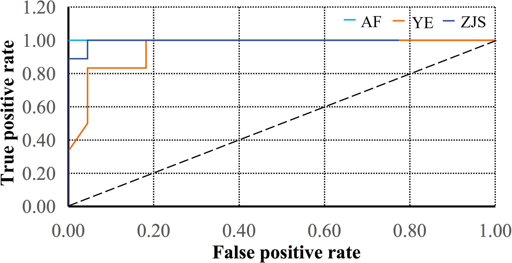
The ROC curves of testing dataset for the groups of farmed (AF), Yangtze River estuary (YE), and Zhongjieshan (ZJS) via random forest algorithms, with the colors of light blue, brown, and deep blue, corresponding to AUC values of 1.00, 0.95, and 0.99, respectively. The black dashed line indicates the performance baseline of random forest algorithm.
In the random forest model, feature importance was used to indicate the contribution of each variable to the model. Among the variables, Hg (0.276) and As (0.255) showed the highest importance, indicating that they contributed significantly to the overall prediction accuracy and node purity of the model. Cd (0.177) also showed relatively high importance, while Fe (0.108) and Cu (0.095) demonstrated moderate importance. Zn (0.088) was of lower importance, indicating that its contribution to the model was relatively small.
4 discussion
4.1 Analysis of trace element concentrations among groups
In previous studies, Marengo et al. (2018) assessed the concentrations of trace elements in Sparus aurata and reported that the average levels of Fe, Cu, Zn, Cd, and As in wild S. aurata were 2.171, 0.200, 3.551, 0.002, and 5.489 mg kg–1, respectively, while in farmed S. aurata, the concentrations of these elements were 2.475, 0.497, 4.345, 0.004, and 2.739 mg kg–1, respectively. They also evaluated the trace element concentrations in Dicentrarchus labrax and conducted a human health risk assessment (Marengo et al., 2018). Alam et al. (2002) measured the concentrations of 13 elements in the muscle, liver, intestine, kidney, and gonads of cultured and wild carp caught in Lake Kasumigaura, Japan, and they suggested that despite their dietary differences, the wild and cultured fish were accumulating and distributing elements in the same manner and that systematic aquaculture practices could effectively regulate most increasing element concentrations in the fish. However, other studies have demonstrated that aquaculture practices, particularly water quality management and feeding strategies, can significantly influence the accumulation of heavy metals in farmed fish (Emenike et al., 2022). Barszcz and Sidoruk (2024) reported that water management practices in aquaculture influenced the accumulation of heavy metals such as Cd and Hg in Oncorhynchus mykiss muscle, posing potential health risks to consumers. Cretì et al. (2010) also reported that Sparus aurat reared in three different aquaculture systems exhibited significant differences in cadmium and lead concentrations in their tissues.
In our study, we compared concentrations of eight trace elements in the muscle tissues of O. fasciatus from three different geographic groups and detected significant differences among the AF, YE, and ZJS groups. Among them, Fe, Cu, Zn, Cd, As, and Hg showed significant differences between two and among three groups, while no significant differences were detected for Mn and Cr. Fe is important in biochemical processes such as oxygen binding and transport as well as electron transfer reactions, and it is absorbed via the gastrointestinal tract. Cu is involved in key physiological and biochemical processes, including cellular energy production and the metabolism of various Cu-containing enzymes and Cu-requiring proteins, and it is absorbed through the gills and digestive tract of fishes (Taylor et al., 2003; Lall and Kaushik, 2021). Fe absorption from aquatic environments is usually relatively inefficient (Bury and Grosell, 2003), thus making differences in food sources a key factor impacting the variation of Fe concentrations among the groups. In addition to dietary differences, water environmental variations among habitats could explain the differences in Cu levels. In the other study, Cu sediment concentrations for the ZJS group ranged from 35 to 40 mg kg–1, which is significantly higher than that 23.9 mg kg–1 of the YE group (Xu et al., 2015).
In addition to Zn, Hg, Cd, and As, Zn and Hg levels were higher in the AF group compared to the two wild groups. Zn is very important to fish health and growth, and it is often added to improve growth performance, hormone regulation, and overall health in aquaculture (Kumar et al, 2018; Sallam et al., 2020; Ibrahim et al., 2022). The continuous diet for the AF group contributed to its higher Zn levels compared to those of the two wild groups. The higher Hg content in the AF group was consistent with the findings from other studies (Table 4), which reported higher Hg concentrations in farmed Acanthopagrus schlegelii (0.077 mg kg–1) and Sebastes schlegelii (0.064 mg kg–1) compared to their wild specimens (0.015 mg kg–1 and 0.057 mg kg–1, respectively) (Kim et al., 2012). However, a different trend was observed in species such as Larimichthys crocea and Pagrus major, in which the Hg concentrations of wild and farmed populations were similar, with both measured at 0.014 mg kg–1 in L. crocea and approximately 0.072 mg kg–1 in P. major (Kim et al., 2012; Zheng et al., 2024), suggesting that differences in diet composition and ecological niche may account for these differences.
Table 4
| Species | Sites | Element (mg kg-1 ww) | Reference | |||||
|---|---|---|---|---|---|---|---|---|
| Fe | Cu | Zn | Cd | As | Hg | |||
| Wild Oplegnathus fasciatus (YE) | Yangtze River Estuary | 4.357 | 0.334 | 2.340 | 0.002 | 1.153 | 0.017 | This study |
| Wild Oplegnathus fasciatus (ZJS) | Zhongjieshan Islands sea area | 7.041 | 0.488 | 2.720 | 0.005 | 1.663 | 0.011 | |
| Farmed Oplegnathus fasciatus (AF) | Zhoushan, China | 4.789 | 0.426 | 2.896 | 0.001 | 0.585 | 0.041 | |
| Wild Sparus aurata | Northwestern Mediterranean | 2.171 | 0.200 | 3.551 | 0.002 | 5.489 | — | Marengo et al. (2018) |
| Farmed Sparus aurata | Corsican coast, France | 2.475 | 0.497 | 4.345 | 0.004 | 2.739 | — | |
| Wild Dicentrarchus labrax | Northwestern Mediterranean | 3.115 | 0.330 | 4.221 | 0.001 | 1.030 | — | |
| Farmed Dicentrarchus labrax | Corsican coast, France | 2.468 | 0.440 | 3.819 | 0.002 | 1.955 | — | |
| Wild Cyprinus carpio | Lake Kasumigaura, Japan | 2.729 | 0.249 | 5.433 | 0.009 | 0.095 | — | Alam et al. (2002) |
| Farmed Cyprinus carpio | 4.125 | 0.332 | 5.449 | 0.007 | 0.179 | — | ||
| Wild Acanthopagrus schlegelii | southern Korean Peninsula | — | — | — | — | — | 0.015 | Kim et al. (2012) |
| Farmed Acanthopagrus schlegelii | — | — | — | — | — | 0.077 | ||
| Wild Sebastes schlegeli | — | — | — | — | — | 0.057 | ||
| Farmed Sebastes schlegeli | — | — | — | — | — | 0.079 | ||
| Wild Mugil cephalus | — | — | — | — | — | 0.006 | ||
| Farmed Mugil cephalus | — | — | — | — | — | 0.024 | ||
| Wild Pagrus major | — | — | — | — | — | 0.072 | ||
| Farmed Pagrus major | — | — | — | — | — | 0.072 | ||
| Wild Larimichthys crocea | Nanji islands, China | — | — | — | — | 0.323 | 0.014 | Zheng et al. (2024) |
| Farmed Larimichthys crocea | — | — | — | — | 0.155 | 0.014 | ||
Concentrations of trace elements in fish muscle of this study and the available literatures.
In contrast, Cd and As concentrations in the two wild groups were higher than those of the AF group, which might be due to the increasing industrial activities and maritime engineering projects adjacent to their natural habitats. Results of several studies have indicated that marine invertebrates absorb As that mimics natural substrates, such as betaine arsenic [(CH3)3As+CH2COO−], which structurally resembles glycine betaine [(CH3)3N+CH2COO−], a molecule exploited by marine invertebrates use to maintain osmotic balance (Amlund and Berntssen, 2004; Clowes and Francesconi, 2004). In contrast, wild O. fasciatus groups primarily feed on marine invertebrates (Zhao et al., 2016). Xu et al. (2015) studied heavy metal concentrations in the sediment around the west side of the Zhoushan fishing ground and reported a median As contamination level in the northern waters of Dongji Islands. However, there were no such reports for the areas of the Yangtze River Estuary (Xu et al., 2019). This may explain why the As concentration in the ZJS wild group was significantly higher than that of the YE group.
Correlation analysis between Fulton’s condition factor (K) and the concentrations of Fe, Cu, Zn, Cd, As and Hg shows that, in most cases, muscle levels of these elements are not significantly related to K, indicating that somatic condition is not a primary driver of their accumulation. Mercury is the clear exception: K exhibits a significant negative correlation with Hg. Similar results have been reported by Piras et al. (2023), who found a negative association between mercury concentration and K in the tissues of Thunnus thynnus. This relationship is commonly attributed to the lipid dilution effect, whereby individuals with higher K values typically exhibit greater lipid reserves, thereby reducing mercury concentrations in muscle tissue (Balshaw et al., 2008). Supporting this hypothesis, previous studies have demonstrated that tissues with higher lipid content consistently exhibit lower mercury levels compared to lean tissues (Ross and Edwards, 2015). Nevertheless, in studies involving interspecific comparisons or trophic-level analyses, large, well-conditioned individuals at higher trophic positions often accumulate greater absolute amounts of mercury (Hernández-Domínguez et al., 2025). In such cases, higher K values may positively correlate with total mercury burden, as these individuals are typically larger and occupy elevated positions within the food web, leading to increased bioaccumulation (Hernández-Domínguez et al., 2025). However, in the ZJS population, no significant correlations were observed between K and any of the measured elements, suggesting that differences in growth dilution associated with individual life history traits may have masked the potential effects of trace element concentrations on somatic condition (Jiang et al., 2022; Liao et al., 2023).
4.2 Group discrimination and model limit usage
Elemental analysis (or elemental fingerprinting, elemental profiling, multi-element analysis) involves analyzing samples from identified groups to quantify element contents to determine if differences in the element concentrations can be combined with chemometrics methods (including cluster analysis, SDA, and random forest model) to classify group membership. The elemental profiles of animal tissues are related to the true elemental profiles of the environments in which they live. In this study, we used cluster analysis, SDA, and the random forest model to distinguish three different groups of O. fasciatus and illustrated the potential of using trace element concentrations as a group discrimination method.
In contrast to SDA and the random forest model, cluster analysis is an unsupervised learning method that does not rely on pre-labeled category information, thus it cannot utilize class labels to optimize classification results (Liu et al., 2012). SDA and the random forest model are supervised and ensemble learning methods, respectively. The former improves classification by stepwise feature selection based on known class information, whereas the latter enhances accuracy through random decision tree construction and automatic feature importance evaluation (Breiman, 2001). The PCA results showed substantial overlap between the YE group and both the AF and ZJS groups, which may explain the poor performance of cluster analysis. In addition, it is worth noting that the classification accuracy of the random forest model exceeded that of traditional statistical analysis (Gopi et al., 2019). Our result further enhance the significant potential of using random forest models as they surpass traditional linear regression analysis for classification tasks (Fernández-Delgado et al., 2014). Through randomly sampling training data and selecting subsets of features, the random forest model significantly enhanced classification potential and noise resistance, effectively preventing overfitting (Dong and Huang, 2013). Compared to traditional statistical methods, the random forest model provided greater flexibility, as it could handle elements with nonlinear relationships and interactions, which are common in biological data (Guisan and Zimmermann, 2000). Although these methods differ due to their analytical principles and underlying logic, they may offer complementary perspectives in terms of variable selection and data structure analysis, thereby enhancing the comprehensiveness and reliability of the classification results.
The methods used in this study showed higher accuracy for the AF group compared to the two wild groups. Cui et al. (2021) reported that Cu achieved a 100% classification rate in identifying salmonids cultured in freshwater and seawater. Li et al. (2019) found that Cr, Mn, and Fe concentrations were higher in shrimp (Litopenaeus vannamei) cultured in freshwater than in those cultured in seawater, and As levels showed the reverse pattern. For discriminating wild and farmed European sea bass (Dicentrarchus labrax), element analysis achieved 100% accuracy (Varrà et al., 2019), further verifying the important role of trace elements in the discrimination of aquatic animal groups. Anderson et al. (2010) also reported that the accuracy of classifying farmed salmon groups was higher than that of wild groups. This result might be related to the controlled farming conditions and stable food supply in aquaculture, whereas groups that live in natural marine environments experience fluctuating environmental conditions and random, unstable food sources. Additionally, Souza et al. (2020) concluded that increasing sample size can effectively enhance model precision. The limitations of this study include the relatively small sample size and the limited number of sampling sites. Future research should expand the spatial coverage of sampling sites between the Yangtze River estuary and Zhongjieshan, increase the number of cultured sites, and enlarge the overall sample size to more comprehensively capture spatial variation in trace element accumulation and to enable a more systematic and rigorous evaluation of classification models. Moreover, the temporal variation in trace element composition following the release of cultured fish into the wild should be considered. Incorporating time-series sampling or additional biological markers in future studies may improve the long-term applicability and robustness of the discrimination approach.
Other studies have also demonstrated that elemental differences among wild groups can effectively reflect their geographic origins. For instance, Varrà et al. (2019) successfully achieved 100% classification of European sea bass from the central Mediterranean, western Mediterranean, and eastern Mediterranean through elemental analysis. Similarly, 100% classification accuracy was achieved for Apostichopus japonicus samples from the Bohai Sea, Yellow Sea, and East China Sea (Liu et al., 2012). Fu et al. (2021) further highlighted the accuracy of elemental analysis, showing that a linear discriminant model trained on ten elements (Fe, Zn, Al, Ni, As, Cr, V, Se, Ca, and Na) could achieve a classification rate of 98.8% for Salmo salar. Additionally, 92% of Cerastoderma edule samples were successfully classified based on their harvesting locations (Ricardo et al., 2015). Duarte et al. (2022) demonstrated that elemental analysis effectively distinguished Raja clavata from four different fishing areas in Portugal. By distinguishing between the wild YE and ZJS groups of O. fasciatus, our results further support the reliability of elemental analysis in geographic group classification. These findings emphasize the potential of elemental profiling as a robust tool for identifying group structure and geographic distribution in wild aquatic species. In the future, we plan to incorporate isotope measurements to further enhance the accuracy of group discrimination.
5 Conclusion
In this study, we performed a comparative analysis of trace element concentrations in the muscle tissues of the regional species O. fasciatus from the AF, YE, and ZJS groups and identified distinct differences among the three groups. Our findings suggest that Fe, Cu, Zn, Cd, As, and Hg play key roles in differentiating these geographic populations, while Mn and Cr contribute minimally to classification accuracy. We found a higher performance efficiency for the random forest model compared to other methods such as cluster analysis and SDA. In future research, we intend to expand the number of sampling sites and integrate additional supporting data, including trace element concentrations in local waters and feed sources, to enhance classification accuracy and strengthen the ecological relevance of our findings, ultimately contributing to the quality and safety of seafood products.
Statements
Data availability statement
The original contributions presented in the study are included in the article/supplementary material. Further inquiries can be directed to the corresponding author.
Ethics statement
The animal study was approved by Institutional Animal Care and Use Committee of Zhejiang Ocean University. The study was conducted in accordance with the local legislation and institutional requirements.
Author contributions
KX: Formal Analysis, Methodology, Project administration, Supervision, Visualization, Writing – original draft, Writing – review & editing. JW: Formal Analysis, Methodology, Writing – original draft. YZ: Resources, Writing – original draft. KZ: Resources, Writing – original draft. GF: Writing – review & editing, Software. HW: Resources, Writing – original draft. JZ: Resources, Writing – original draft.
Funding
The author(s) declare that financial support was received for the research and/or publication of this article. This study was supported by National Key R&D Program of China (2019YFD0901204), and the Zhejiang Provincial Key R&D Program (2019C02056).
Acknowledgments
The authors express their gratitude to the staff of the Zhejiang Marine Fisheries Research Institute.
Conflict of interest
The authors declare that the research was conducted in the absence of any commercial or financial relationships that could be construed as a potential conflict of interest.
Generative AI statement
The author(s) declare that no Generative AI was used in the creation of this manuscript.
Publisher’s note
All claims expressed in this article are solely those of the authors and do not necessarily represent those of their affiliated organizations, or those of the publisher, the editors and the reviewers. Any product that may be evaluated in this article, or claim that may be made by its manufacturer, is not guaranteed or endorsed by the publisher.
References
1
Alam M. G. M. Tanaka A. Allinson G. Laurenson L. J. B. Stagnitti F. Snow E. T. (2002). A comparison of trace element concentrations in cultured and wild carp (Cyprinus carpio) of Lake Kasumigaura, Japan. Ecotoxicology Environ. Saf.53, 348–354. doi: 10.1016/S0147-6513(02)00012-X
2
Amlund H. Berntssen M. H. G. (2004). Arsenobetaine in Atlantic salmon (Salmo salar L.): influence of seawater adaptation. Comp. Biochem. Physiol. Part C: Toxicol. Pharmacol.138, 507–514. doi: 10.1016/j.cca.2004.08.010
3
Anderson K. A. Hobbie K. A. Smith B. W. (2010). Chemical profiling with modeling differentiates wild and farm-raised salmon. J. Agric. Food Chem.58, 11768–11774. doi: 10.1021/jf102046b
4
Balshaw S. Edwards J. W. Ross K. E. Daughtry B. J. (2008). Mercury distribution in the muscular tissue of farmed southern bluefin tuna (Thunnus maccoyii) is inversely related to the lipid content of tissues. Food Chem.111, 616–621. doi: 10.1016/j.foodchem.2008.04.041
5
Barszcz A. A. Sidoruk M. (2024). Impacts of water management in aquaculture on heavy metal accumulation in rainbow trout muscles and associated health risks from consumption. Food Control164, 110617. doi: 10.1016/j.foodcont.2024.110617
6
Breiman L. (2001). Random forests. Mach. Learn.45, 5–32. doi: 10.1023/A:1010933404324
7
Bury N. Grosell M. (2003). Iron acquisition by teleost fish. Comp. Biochem. Physiol. Part C: Toxicol. Pharmacol.135, 97–105. doi: 10.1016/S1532-0456(03)00021-8
8
Clowes L. A. Francesconi K. A. (2004). Uptake and elimination of arsenobetaine by the mussel Mytilus edulis is related to salinity. Comp. Biochem. Physiol. Part C: Toxicol. Pharmacol.137, 35–42. doi: 10.1016/j.cca.2003.11.003
9
Cretì P. Trinchella F. Scudiero R. (2010). Heavy metal bioaccumulation and metallothionein content in tissues of the sea bream Sparus aurata from three different fish farming systems. Environ. Monit. Assess.165, 321–329. doi: 10.1007/s10661-009-0948-z
10
Cui H. Dong S. Li L. Gao Q. Zhou Y. (2021). Evaluation of elemental analysis assisted by chemometrics for authenticating production methods and geographical origins of salmonids. Aquaculture545, 737210. doi: 10.1016/j.aquaculture.2021.737210
11
Dong S. S. Huang Z. X. (2013). A brief theoretical overview of random forests. J. Integr. Technol.2, 1–7.
12
Duarte B. Duarte I. A. Caçador I. Reis-Santos P. Vasconcelos R. P. Gameiro C. et al . (2022). Elemental fingerprinting of thornback ray (Raja clavata) muscle tissue as a tracer for provenance and food safety assessment. Food Control133, 108592. doi: 10.1016/j.foodcont.2021.108592
13
Emenike E. C. Iwuozor K. O. Anidiobi S. U. (2022). Heavy metal pollution in aquaculture: Sources, impacts and mitigation techniques. Biol. Trace Element Res.200, 4476–4492. doi: 10.1007/s12011-021-03037-x
14
Fernández-Delgado M. Cernadas E. Barro S. Amorim D. (2014). Do we need hundreds of classifiers to solve real-world classification problems? J. Mach. Learn. Res.15, 3133–3181.
15
Fu X. Hong X. Liao J. Ji Q. Li C. Zhang M. et al . (2021). Fingerprint approaches coupled with chemometrics to discriminate geographic origin of imported salmon in China’s consumer market. Foods10, 2986. doi: 10.3390/foods10122986
16
Gopi K. Mazumder D. Sammut J. Saintilan N. Crawford J. Gadd P. (2019). Isotopic and elemental profiling to trace the geographic origins of farmed and wild-caught Asian seabass (Lates calcarifer). Aquaculture502, 56–62. doi: 10.1016/j.aquaculture.2018.12.012
17
Guisan A. Zimmermann N. E. (2000). Predictive habitat distribution models in ecology. Ecol. Model.135, 147–186. doi: 10.1016/S0304-3800(00)00354-9
18
Hernández-Domínguez C. Bjedov D. Buelvas-Soto J. Córdoba-Tovar L. Bernal-Alviz J. Marrugo-Negrete J. (2025). Factors affecting arsenic and mercury accumulation in fish from the Colombian Caribbean: A multifactorial approach using machine learning. Environ. Res.268, 120761. doi: 10.1016/j.envres.2025.120761
19
Ibrahim M. S. El-Gendi G. M. I. Ahmed A. I. El-Haroun E. R. Hassaan M. S. (2022). Nano zinc versus bulk zinc form as dietary supplied: effects on growth, intestinal enzymes and topography, and hemato-biochemical and oxidative stress biomarker in Nile tilapia (Oreochromis niloticus Linnaeus 1758). Biol. Trace Element Res.200, 1347–1360. doi: 10.1007/s12011-021-02724-z
20
Iguchi J. Isshiki M. Takashima Y. Yamashita Y. Yamashita M. (2014). Identifying the origin of Corbicula clams using trace element analysis. Fisheries Sci.80, 1089–1096. doi: 10.1007/s12562-014-0775-1
21
Jiang X. Wang J. Pan B. Li D. Wang Y. Liu X. (2022). Assessment of heavy metal accumulation in freshwater fish of Dongting Lake, China: Effects of feeding habits, habitat preferences and body size. J. Environ. Sci.112, 355–365. doi: 10.1016/j.jes.2021.05.004
22
Kim C. K. Lee T. W. Lee K. T. Lee J. H. Lee C. B. (2012). Nationwide monitoring of mercury in wild and farmed fish from fresh and coastal waters of Korea. Chemosphere89, 1360–1368. doi: 10.1016/j.chemosphere.2012.05.093
23
Korkmaz C. Ay Ö. Çolakfakıoğlu C. Erdem C. (2019). Heavy metal levels in some edible crustacean and mollusk species marketed in Mersin. Thalassas35, 65–71. doi: 10.1007/s41208-018-0086-x
24
Kumar N. Krishnani K. K. Singh N. P. (2018). Effect of dietary zinc-nanoparticles on growth performance, anti-oxidative and immunological status of fish reared under multiple stressors. Biol. Trace Element Res.186, 267–278. doi: 10.1007/s12011-018-1285-2
25
LaBine G. O. Molloy P. P. Christensen J. R. (2021). Determination of elemental composition in soft biological tissue using laser ablation inductively coupled plasma mass spectrometry: method validation. Appl. Spectrosc.75, 1262. doi: 10.1177/00037028211008535
26
Lall S. P. Kaushik S. J. (2021). Nutrition and metabolism of minerals in fish. Animals11, 2711. doi: 10.3390/ani11092711
27
Li L. Boyd C. E. Dong S. (2015). Chemical profiling with modeling differentiates Ictalurid catfish produced in fertilized and feeding ponds. Food Control50, 18–22. doi: 10.1016/j.foodcont.2014.08.014
28
Li L. Boyd C. E. Odom J. (2014). Identification of Pacific white shrimp (Litopenaeus vannamei) to rearing location using elemental profiling. Food Control45, 70–75. doi: 10.1016/j.foodcont.2014.03.013
29
Li L. Cui H. Dong S. Boyd C. E. (2019). Use of elemental profiling and isotopic signatures to differentiate Pacific white shrimp (Litopenaeus vannamei) from freshwater and seawater culture areas. Food Control95, 249–256. doi: 10.1016/j.foodcont.2018.08.015
30
Li S. L. Xu D. D. Lou B. Wang W. D. Xin J. Mao G. M. et al . (2012). The genetic diversity of wild and hatchery-released Oplegnathus fasciatus from inshore water of Zhoushan revealed by AFLP. Mar. Sci.36, 21–27.
31
Liao Z. Li Z. Wu M. Zeng K. Han H. Li C. et al . (2023). Trace metal exposure and risk assessment of local dominant fish species in the Beijiang River Basin of China: A 60 years’ follow-up study. Sci. Total Environ.904, 166322. doi: 10.1016/j.scitotenv.2023.166322
32
Liu M. H. Liang J. Xu H. X. (2020). Spatio-temporal niche of dominant shrimp species in the Zhongjieshan Islands Marine Protected Area, China. Chin. J. Appl. Ecol.31, 1746–1752. doi: 10.13287/j.1001-9332.202005.036
33
Liu X. Xue C. Wang Y. Li Z. Xue Y. Xu J. (2012). The classification of sea cucumber (Apostichopus japonicus) according to region of origin using multi-element analysis and pattern recognition techniques. Food Control23, 522–527. doi: 10.1016/j.foodcont.2011.08.025
34
Marengo M. Durieux E. D. H. Ternengo S. Lejeune P. Degrange E. Pasqualini V. et al . (2018). Comparison of elemental composition in two wild and cultured marine fish and potential risks to human health. Ecotoxicology Environ. Saf.158, 204–212. doi: 10.1016/j.ecoenv.2018.04.034
35
Milatou N. Megalofonou P. (2014). Age structure and growth of bluefin tuna (Thunnus thynnus, L.) in the capture-based aquaculture in the Mediterranean Sea. Aquaculture424–425, 35–44. doi: 10.1016/j.aquaculture.2013.12.037
36
Ni M. L. Qiu Z. C. Li Y. H. Huang Q. M. (2020). Determination of 12 elements in deep-sea fish muscles by ICP-MS after pretreatment of microwave digestion. Sci. Technol. Food Industry41, 244–249. doi: 10.13386/j.issn1002-0306.2020.09.039
37
Nygaard R. Roll K. H. (2024). Cross-hedging wild salmon prices. J. Commodity Markets33, 100390. doi: 10.1016/j.jcomm.2024.100390
38
Piras P. Macciotta N. P. P. Meloni D. Sanna A. Cossu M. Salis S. et al . (2023). Effects of age, Fulton’s condition index (K) and muscle fat on total mercury content in raw, pre-canning and canned samples of Atlantic bluefin tuna (Thunnus thynnus). Foods12, 2686. doi: 10.3390/foods12142686
39
Ricardo F. Génio L. Costa Leal M. Albuquerque R. Queiroga H. Rosa R. et al . (2015). Trace element fingerprinting of cockle (Cerastoderma edule) shells can reveal harvesting location in adjacent areas. Sci. Rep.5, 11932. doi: 10.1038/srep11932
40
Ross K. Edwards J. (2015). Spatial variation in the mercury concentration of muscle myomeres in steaks of farmed southern bluefin tuna. Foods4, 254–262. doi: 10.3390/foods4020254
41
Sallam A. E. Mansour A. T. Alsaqufi A. S. Salem M. E. S. (2020). Growth performance, anti-oxidative status, innate immunity, and ammonia stress resistance of Siganus rivulatus fed diet supplemented with zinc and zinc. Aquaculture Rep.18, 100410. doi: 10.1016/j.aqrep.2020.100410
42
Souza A. T. Soukalová K. Děd V. Šmejkal M. Moraes K. Říha M. et al . (2020). Otolith shape variations between artificially stocked and autochthonous pikeperch (Sander lucioperca). Fisheries Res.231, 105708. doi: 10.1016/j.fishres.2020.105708
43
Taylor L. N. Wood C. M. McDonald D. G. (2003). An evaluation of sodium loss and gill metal binding properties in rainbow trout and yellow perch to explain species differences in copper tolerance. J. Exp. Biol.22, 2159–2166. doi: 10.1897/02-256
44
Varrà M. O. Ghidini S. Zanardi E. Badiani A. Ianieri A. (2019). Authentication of European sea bass according to production method and geographical origin by light stable isotope ratio and rare earth elements analyses combined with chemometrics. Ital. J. Food Saf.8, 7872. doi: 10.4081/ijfs.2019.7872
45
Wang H. X. Xu K. D. Zhou Y. D. Chen L. Li P. F. Xu G. Q. et al . (2022). Investigation of a mark-recapture method of Oplegnathus fasciatus in the waters of northern Zhejiang. J. Zhejiang Ocean Univ. (Natural Sci. Edition)41, 455–458. doi: 10.3969/j.issn.1008-830X.2022.05.013
46
Wang J. H. Hu G. S. Wu Z. Zhu K. Xu K. D. Wang H. X. et al . (2024a). Analysis of morphological differences between natural and cultured populations of Oplegnathus fasciatus. J. Zhejiang Univ. (Agriculture Life Sciences)50, 817–826. doi: 10.3785/j.issn.1008-9209.2023.11.161
47
Wang J. H. Zhu K. Xu K. D. Wang H. X. Chen R. Y. Zeng J. Y. (2024b). Discrimination of natural and cultured Oplegnathus fasciatus populations in Zhoushan sea area based on otolith morphology. Chin. J. Appl. Ecol.35, 3165–3173. doi: 10.13287/j.1001-9332.202411.029
48
Xu G. Liu J. Pei S. F. Hu G. Kong H. H. (2015). Geochemical background and ecological risk of heavy metals in surface sediments from the west Zhoushan Fishing Ground of East China Sea. Environ. Sci. pollut. Res.22, 20283–20294. doi: 10.1007/s11356-015-5662-5
49
Xu C. Wang S. K. Zhao F. Yang G. Zhuang P. (2019). Trophic structure of food web and its variation on aquatic animals in the Yangtze Estuary. Acta Hydrobiologica Sin.43, 155–164. doi: 10.7541/2019.019
50
Zhao S. L. Xu H. X. Zhong J. S. Chen J. (2016). “(,” in Fauna of marine fishes in zhejiang, vol. 1. (Zhejiang Science and Technology Publishing House, Zhejiang, China), 726–727.
51
Zheng J. L. Chen Y. L. Wan F. G. Zhan Q. H. Chen T. H. Chen S. et al . (2024). Comparative study on the quality of wild and ecologically farmed large yellow croaker through on-site synchronous sampling from the Nanji Archipelago in the East China Sea. Aquaculture591, 741098. doi: 10.1016/j.aquaculture.2024.741098
Summary
Keywords
parrotfish, Northwest Pacific, aquatic animal, Zhoushan islands, trace elements, ROC, AUC
Citation
Xu K, Wang J, Zhou Y, Zhu K, Fang G, Wang H and Zeng J (2025) A group identification method based on trace element levels of muscle tissue: a case study for Oplegnathus fasciatus in the Northern Zhejiang Waters. Front. Mar. Sci. 12:1627012. doi: 10.3389/fmars.2025.1627012
Received
12 May 2025
Accepted
04 July 2025
Published
21 July 2025
Volume
12 - 2025
Edited by
Peter Goethals, Ghent University, Belgium
Reviewed by
Yuan Li, State Oceanic Administration, China
Qihua Pang, South China Normal University, China
Updates
Copyright
© 2025 Xu, Wang, Zhou, Zhu, Fang, Wang and Zeng.
This is an open-access article distributed under the terms of the Creative Commons Attribution License (CC BY). The use, distribution or reproduction in other forums is permitted, provided the original author(s) and the copyright owner(s) are credited and that the original publication in this journal is cited, in accordance with accepted academic practice. No use, distribution or reproduction is permitted which does not comply with these terms.
*Correspondence: Kaida Xu, xkd1981@zjou.edu.cn
†These authors have contributed equally to this work
Disclaimer
All claims expressed in this article are solely those of the authors and do not necessarily represent those of their affiliated organizations, or those of the publisher, the editors and the reviewers. Any product that may be evaluated in this article or claim that may be made by its manufacturer is not guaranteed or endorsed by the publisher.