Analysis of infragravity waves characteristics and energy evaluation based on field observations

The characteristics and energies of infragravity waves (IGWs) are investigated based on field observations. IGWs are closely related to short waves, and the wave spectrum integration method was adopted to separate sea and swell waves. By comparing the performance of the separation frequency in the spectral shape and the correlation between the IGWs and short waves, it was found that the dynamic separation frequency was more reasonable than the commonly used fixed separation frequencies (0.125 and 0.14 Hz). Infragravity waves exhibited a stronger correlation with swell than with wind waves, with a correlation coefficient exceeding 0.8. Therefore, swell wave heights were used instead of short-wave heights for the energy evaluation of the IGWs. The spectral domain method was adopted to separate the incident and reflected IGWs, and, combined with the bound infragravity waves (BIG), was used to obtain the wave height of each IGW component. The wave heights of the BIG and swell exhibited a significant quadratic relationship. The correlation between the free infragravity waves (FIG) and swell was weaker than that of the BIG. An empirical expression between the wave heights of total incident IGWs and the swell waves was obtained, and the exponent α related to swell wave heights was approximately 1.0.

1 Introduction

In the ocean, the typical wave frequency range is from 0.04 to 1.0 Hz, and these waves are called gravity waves (Bertin et al., 2018; Holthuijsen, 2007). Infragravity waves (hereafter IGWs) refer to waves with frequencies lower than the common short waves in the ocean, with a frequency range of 0.004 to 0.04 Hz (Bertin et al., 2018). Under identical wave height and water depth conditions, the wavelengths of IGWs are much larger. IGWs are also called low-frequency long waves (Dong et al., 2020; Gao et al., 2019).

There are three main generation mechanisms for IGWs: the release of bound infragravity waves, movement of the breaking point, and bore merging in the surf zone (Bertin et al., 2018). In general, the intensity of IGWs is much lower than that of sea and swell waves in the ocean. However, the energy of IGWs cannot be ignored under the following conditions. First, as the waves travel inshore, short-wave energy dissipates in the surf zone through wave breaking processes. In contrast, the energy of released bound IGWs increases with increasing wave nonlinearity, resulting in the relative wave energy of the IGWs being larger than that of short waves near the shore (Matsuba et al., 2021; Roeber and Bricker, 2015; Zheng et al., 2021). Secondly, under extreme ocean conditions during typhoons, swells triggered by typhoons can excite considerable levels of IGWs. Matsuba et al. (2020) observed that the wave height of IGWs could reach 2.0 m near the coast of Seisho during a typhoon. Studies have demonstrated that IGWs play a significant role in nearshore hydrodynamics, such as wave run-up, nearshore sediment movement, beach and dune erosion, and harbor oscillations (Bertin et al., 2018; Dong et al., 2020; Holman and Bowen, 1982; Smith and Mocke, 2002). There is a close relationship between IGWs and nearshore sediment movement, especially under extreme ocean conditions such as storms. Smith and Mocke (2002) found that the frequencies of incipient motion and oscillation of nearshore sediments are equal to the frequencies of the IGW band and not those of the incident short-wave group band. Mendes et al. (2020) observed that sediment transport and shoreline changes were mainly caused by strong IGWs generated by the breaking of short waves with large wave heights during Storm Leslie. The wavelength of IGWs was close to the characteristic scale of the harbor (0.5–5 km), and the period was close to the intrinsic period of moored ships (Dong et al., 2020). Therefore, IGWs cause harbor oscillation (Gao et al., 2024, 2021, 2020, 2023), which lead to violent movements of moored ship and seriously affect loading and unloading efficiency. For example, in Sendai New Harbor, Japan, moored ships continuously sway under the influence of IGWs, which made them unable to operate normally (Nagai et al., 1994). Consequently, it is crucial to study the wave characteristics of IGWs and evaluate its energy.

Based on study of the correlation between IGWs and short waves, the quantitative relationship between the wave characteristic parameters of the short-wave group and the wave height of IGWs has been proposed. The energy of the IGWs can be deduced from short-wave characteristic parameters which are easy to measure. Numerous studies based on field observations have proposed empirical formula for the relationship between the wave height of IGWs and the characteristic parameters of short waves (Dong et al., 2024; Herbers et al., 1994; Medina, 1990; Nelson et al., 1988; Okihiro et al., 1992; Vis et al., 1985). These empirical formulas were mostly used to predict the wave height of IGWs by combining wave height, wave period, and water depth. Nevertheless, the empirical constants in these formulas vary depending on the proximity of the measurements to the port (Lara et al., 2002). Bowers (1992) proposed a simplified empirical formula based on observations at finite water depths in which the effect of water depth was omitted. Based on considerable in-situ measurements, researchers have found that the correlation between IGWs and swell waves is stronger than that with sea waves (Elgar et al., 1992; Ruessink, 1998a). Mahmoudof and Siadatmousavi (2020) presented the correlation between IGWs and sea and swell waves in different wave conditions based on field observations. For non-breaking condition, the correlations of IGWs with swell and sea waves were considerable. For breaking waves, a negligible correlation was observed between bound IGWs and wind waves. Lara et al. (2002) investigated the relationship between four swell wave spectral parameters and the energy of IGWs based on wave data observed by pressure sensors and proposed a method to predict the energy of IGWs from measured pressure data. Given a wave spectrum, the wave height and spectral peak period of the corresponding IGWs can be obtained. However, the correlation between the predicted spectral peak period and the measured values is weak. Ardhuin et al. (2014) proposed that the wave height of IGWs in deep water is strongly correlated with the short-wave height and mean period, and found that the maximum wave height of IGWs corresponds to the maximum short-wave mean period. Dong et al. (2024) found that IGWs are primarily excited by incident swell waves and that an accurate prediction of the IGWs wave height can be achieved using the parameter H_s²T_m-1,0.

The above studies on the quantitative relationship between IGWs and short-wave parameters have limitations, mainly because of the complexity of the wave components. Although several studies have considered the correlations between wind and swell waves with IGWs, a fixed segmentation frequency (0.125 or 0.14 Hz) was typically used to distinguish sea and swell waves (Mahmoudof, 2018). However, it is evident that this separation method cannot satisfy all sea conditions. Based on field observation data, researchers have proposed a variety of sea and swell waves separation methods based on one-dimensional wave spectrum, such as PM method (Earle, 1984), the wave steepness function method (Wang and Hwang, 2001), and wave spectrum integration method (Hwang et al., 2012). The components of IGWs are equally complex, including incident-bound IGWs generated by the nonlinear interaction of short-wave group, onshore incident free IGWs, and offshore reflected free IGWs (Baldock et al., 2000). Separation of these components is an important prerequisite for evaluating the energy of IGWs correctly; whether to separate these components and the separation effect will directly affect the evaluation result of the IGWs energy. Several methods have been developed to separate IGWs (Bertin et al., 2018). In general, they can be divided into time-domain method (Guza et al., 1984), spectral-domain methods (Sheremet et al., 2002; Van Dongeren et al., 2007), and the recently revisited Radon transform methods (Almar et al., 2014). Suitable separation methods can be selected according to the type of observation data. Matsuba et al. (2022) presented the conventional reconstruction method of directional spectra relying on linear wave theory is applicable only in shallow water and proposed a novel method to estimate directional distributions of IGWs.

Previous studies have not concurrently separated short-wave components (wind and swell waves) and IGWs components. In addition, a fixed segmentation frequency (0.125 or 0.14 Hz) was adopted to separate the sea and swell waves, which limits the accuracy of the energy evaluations. The limitations of the previous IGWs characteristics analysis and energy evaluation were studied in this paper. Instead of a fixed frequency, the wave spectrum integration method (Hwang et al., 2012) was adopted to separate sea and swell waves, and the results were compared with those of two fixed frequencies. The second-order nonlinear theory (Hasselmann, 1962) and the spectral-domain separation method (Sheremet et al., 2002) were adopted to separate the components of the IGWs, and the wave height of the bound IGWs and incident and reflected free IGWs were obtained. Subsequently, the energy of each IGWs component was evaluated using the characteristic parameters of the swell waves.

The remainder of this paper is organized as follows. The setup for field measurements, analysis methods, and basic descriptions of the observed wave conditions are presented in Section 2. The results and discussion are presented in Sections 3 through 5. Finally, the conclusions are presented in Section 6.

2 Field observation setup and analysis methods

IGWs have a long period and small amplitude, and their propagation and evolution mechanisms are complicated. Significant IGWs can be excited after strong nonlinear interactions or even the breaking of short waves. Physical modeling and numerical simulation methods have their limitations. The limited size of the water tank in laboratory tests hampers the elimination of reflected long waves' effects, and numerical models overestimate the energy and period parameters of IGWs, which may lead to inaccurate results (De Bakker et al., 2014; Mahmoudof and Takami, 2022). Thus, in-situ observations are the most direct and accurate methods to investigate the characteristics of IGWs. The amplitudes of IGWs are much smaller than those of sea and swell waves and require accurate observation on a stable platform (Dolenc et al., 2008, 2005; Godin et al., 2013; Sugioka et al., 2010).

2.1 Field observation location and setup

The wave data used in this study were measured at Chancay Bay, Peru, on the Pacific coast. An Acoustic Doppler Current Profiler (ADCP) is a type of ocean observation equipment widely used in ocean engineering, environmental science, and resource technology. High quality information on the wave surface, wave direction and ocean current can be obtained, using Acoustic Surface Tracking (AST). The Acoustic Wave and Current (AWAC) is a representative instrument combining ADCP technology with wave measurement capabilities and is widely used to observe IGWs. It was deployed on the seabed for IGWs observations to avoid the influence and damage caused by storms and ship navigation. The locations of measurement station were shown in Figure 1. Under the influence of the Roaring Forties, long-period swell and IGWs occur throughout the year in this sea area (Prevosto et al., 2013), the tidal range was insignificant and the profile changes were negligible. Given the wave characteristics and the limitations due to high observation costs, the field measurements lasted for six months, from July 7 to December 7, 2018. During the measurement process, the position of the measurement point has changed once. The positions of the measurement points and the observation information are listed in Table 1. The sensor was set to collect 4,096 s of wave surface data every 2 hours with a sampling frequency of 4 Hz. After filtering and removing abnormal data, the final dataset consisted of 1,757 samples.

Figure 1

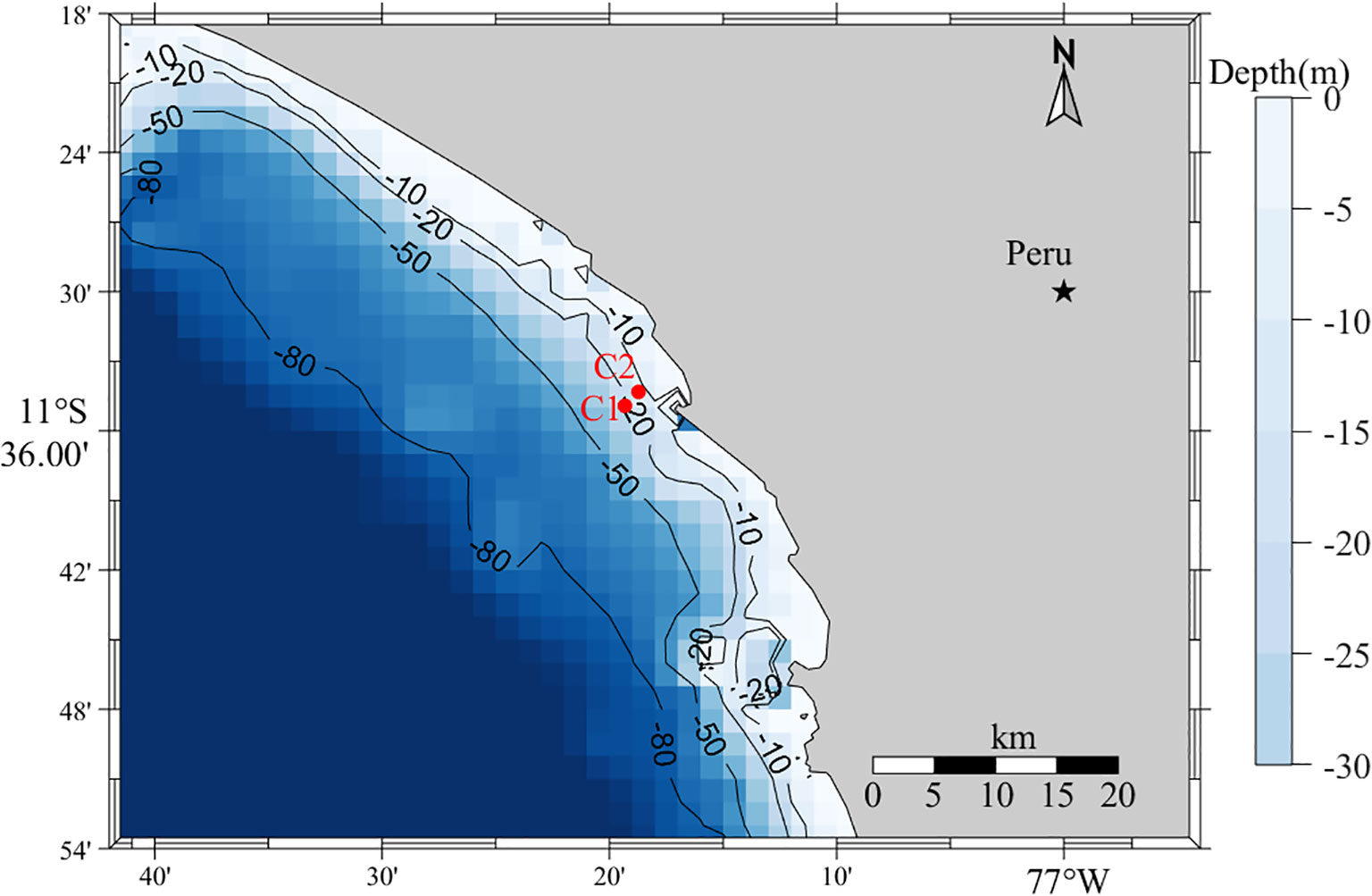
Figure 1. Location of measurement station in Chancay Bay.

Table 1

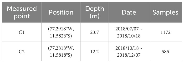
Table 1. Setup and information of the field measurements in Chancay Bay.

2.2 Analysis methods

2.2.1 Separation methods of sea and swell waves

It is imperative to determine the separation frequency between sea and swell waves when researching the correlation between IGWs and sea and swell, so that the wave components can be classified and the energy of each component can be evaluated (Mahmoudof, 2018). Wang and Hwang (2001) proposed a method that required only a one-dimensional (1D) wave spectrum to obtain the separation frequency and defined the wave steepness function to identify sea and swell waves. Hwang et al. (2012) argued that the wave steepness function ignores the growth state of waves, leading to inaccurate separation results. In their method, $S(f)$ in the wave-steepness function was replaced by $S(f)/f^b$, eliminating the influence of the high-frequency part of the spectra on the separation results. The physical meaning corresponding to the improved relation is no longer the average wave steepness but the wave spectrum integration; thus, it is called wave spectrum integration method, which is defined as follows:

$\begin{array}{ll}{I}_b(f_{*})=\frac{{\displaystyle {\int }_{f_{*}}^{f_u}{f}^2[S(f)/f^b]df}}{\sqrt{{\displaystyle {\int }_{f_{*}}^{f_u}[S(f)/f^b]df}}}& (1)\end{array}$

where f is the frequency, $I_b(f_{*})$ is the wave-spectrum integration of frequency $f_{*}$, $f_u$ is the upper integral frequency, and the $S(f)$ is the spectral energy density. By analyzing the spectral characteristics, it is convenient to separate the sea and swell waves when the constant b equal to 1.0, the original Equation 1 is transformed into Equation 2:

$\begin{array}{ll}{I}_1(f_{*})=\frac{{\displaystyle {\int }_{f_{*}}^{f_u}fS(f)df}}{\sqrt{{\displaystyle {\int }_{f_{*}}^{f_u}{f}^{-1}S(f)df}}}& (2)\end{array}$

The frequency corresponding to the maximum value of $I_1(f_{*})$ is the peak frequency $f_m$. Based on the field observation data, the empirical formula between the separation frequency $f_s$ and peak frequency $f_m$ is as follows (see Equation 3):

$\begin{array}{ll}{f}_{\text{s}}=24.2084f_{\text{m}}^3-9.2021f_{\text{m}}^2+1.8906f_{\text{m}}-0.04286& (3)\end{array}$

After obtaining the separation frequency using the above method, the significant wave heights for each wave band were calculated as follows (see Equations 4–6):

$\begin{array}{ll}{H}_{\text{IGWs}}=4.0\sqrt{{\displaystyle {\int }_{0.004}^{0.04}S(f)\text{d}f}}& (4)\end{array}$

$\begin{array}{ll}{H}_{\text{swell}}=4.0\sqrt{{\displaystyle {\int }_{0.04}^{f_{\text{s}}}S(f)\text{d}f}}& (5)\end{array}$

$\begin{array}{ll}{H}_{\text{sea}}=4.0\sqrt{{\displaystyle {\int }_{f_{\text{s}}}^{0.33}S(f)\text{d}f}}& (6)\end{array}$

where H_IGWs, H_swell and H_sea represent the significant wave heights of IGWs, swell waves, and sea waves, respectively.

2.2.2 Surface elevation of bound infragravity waves

Hasselmann (1962) proposed that bound IGWs are the result of the nonlinear interaction of two wave components with similar frequencies in the short-wave group, and derived an analytical expression of the bound IGWs based on weakly second-order nonlinear theory. The subharmonic component forced by two free-wave components at frequencies f_i and f_j is (Li et al., 2020):

$\begin{array}{ll}{\eta }_{ij}=D_{ij}{a}_i{a}_j\cos ({\phi }_i-{\phi }_j)& (7)\end{array}$

where a_i and a_j are the amplitudes of the forcing components, and φ_i and φ_j are the phases. The interaction coefficient D_ij is expressed as follows:

$\begin{array}{ll}{D}_{ij}=-\frac{g{k}_i{k}_j}{2{\omega }_i{\omega }_j}+\frac{{\omega }_i^2-{\omega }_i{\omega }_j+{\omega }_j^2}{2g}-C\frac{g({\omega }_i-{\omega }_j)}{{\omega }_i{\omega }_j[g{k}_{ij}\tanh (k_{ij}h)-{({\omega }_i-{\omega }_j)}^2]}& (8)\end{array}$

where ω = 2πf is the angular frequency, k_ij = | k_i−k_j| is the wave number of the subharmonic component, and h is the water depth. The coefficient C is given by:

$\begin{array}{ll}C=({\omega }_i-{\omega }_j)\left(\frac{{\omega }_i^2{\omega }_j^2}{g^2}+k_i{k}_j\right)-\frac{1}{2}\left[\frac{{\omega }_i{k}_j^2}{{\cosh }^2(k_{j}h)}-\frac{{\omega }_j{k}_i^2}{{\cosh }^2(k_{i}h)}\right]& (9)\end{array}$

The wave amplitude of each frequency component was obtained by Fast Fourier Transform (FFT), and the components with $0.5f_{\text{p}}\le f\le 1.5f_{\text{p}}$ frequencies were selected as the primary components to force subharmonics. By adding the subharmonics generated by all the pairs of components, the total surface elevation of the BIG can be obtained as follows:

$\begin{array}{ll}{\eta }_{\text{BIG}}={\displaystyle \sum _{f_i=0.5f_{\text{p}}}^{1.5f_{\text{p}}}{\displaystyle \sum _{f_j=f_{i+1}}^{1.5f_{\text{p}}}{\eta }_{ij}}}& (10)\end{array}$

FFT was applied to the BIG wave surface, and then the wave height of BIG are calculated as follows:

$\begin{array}{ll}{H}_{\text{BIG}}=4.0\sqrt{{\displaystyle {\int }_{0.004}^{0.04}{S}_{\text{BIG}}(f)\text{d}f}}& (11)\end{array}$

The wave height of FIG was calculated using the difference between Equations 4, 11, as follows:

$\begin{array}{ll}{H}_{\text{FIG}}=\sqrt{H_{{}_{\text{IGWs}}}^2-H_{{}_{\text{BIG}}}^2}& (12)\end{array}$

2.2.3 Separation methods of infragravity waves

Guza et al. (1984) developed a time-domain approach to construct the incident and reflected surface elevations of IGWs based on co-located wave gauges and velocity meters (see Equation 13):

$\begin{array}{ll}{\eta }^{\pm }=\frac{\eta \pm {(h/g)}^{1/2}u}{2}& (13)\end{array}$

where g is the gravitational acceleration, u is the velocity of water particles caused by waves, $\eta$ is the surface elevation of the short-wave group, and ${\eta }^{\pm }$ is the incoming and outgoing IGWs surface elevations. Sheremet et al. (2002) proposed a spectral-domain separation method based on the above expression. Under the assumption of a positive incidence, the energy distribution expression $N^{\pm }(f)$ of the incoming and outgoing IGWs is as follows:

$\begin{array}{ll}{N}^{\pm }(f)=\frac{1}{4}\left[C_{\eta \eta }(f)+\frac{h}{g}{C}_{uu}(f)\pm \left(2\sqrt{\frac{h}{g}}\right)C_{\eta u}(f)\right],& (14)\end{array}$

where $C_{\eta u}$ is the η-u co-spectrum, and $C_{\eta \eta }$ and $C_{uu}$ are η and u auto-spectra, respectively.

Each time series of data was separated into eight segments with 50% overlap in order to diminish the variance. Tapering each ensemble with a Hanning window and averaging the spectra over 16 frequencies resulted in a frequency resolution of 0.0156 Hz and 120 degrees of freedom. The energy fluxes of the incoming and outgoing IGWs were calculated by integrating in the IGWs band, and the reflection coefficient $R_{\text{IGWs}}$ was defined as follows:

$\begin{array}{ll}{F}^{\pm }={\displaystyle {\int }_{0.004}^{0.04}{N}^{\pm }}(f)\sqrt{gh}\text{ d}f& (15)\end{array}$

$\begin{array}{ll}{R}_{\text{IGWs}}=\sqrt{F^{-}/F^{+}}& (16)\end{array}$

2.3 Overview of the wave conditions

During the observation period, there were no typhoons or other abnormal weather. The wave surface of the BIG can be obtained by using Equations 7–10. The wave height of the BIG and FIG can be calculated based on Equations 11, 12, and the significant wave heights of the short waves and various components IGWs were shown in Figure 2. A strong correlation was found between the wave height of the IGWs and that of the short waves.

Figure 2

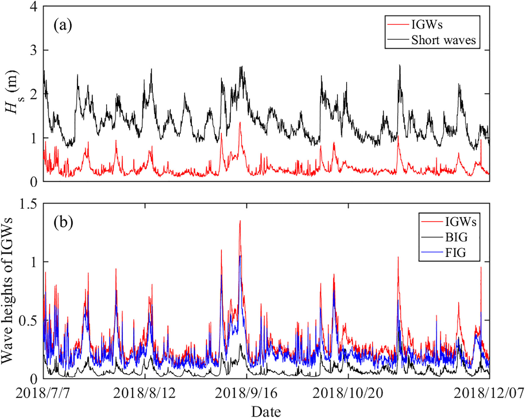
Figure 2. Significant wave height H_s of the short waves (a) and various components IGWs (b).

According to the wave rose diagram (Figure 3), this area was primarily affected by southwest waves, and both the normal and strong wave directions were southwest. The shoreline is approximately northeast (Figure 1), thus, the waves can be regarded as normally incident. The wave spectra consist of more than one component, including local sea wave systems and offshore swell systems.

Figure 3

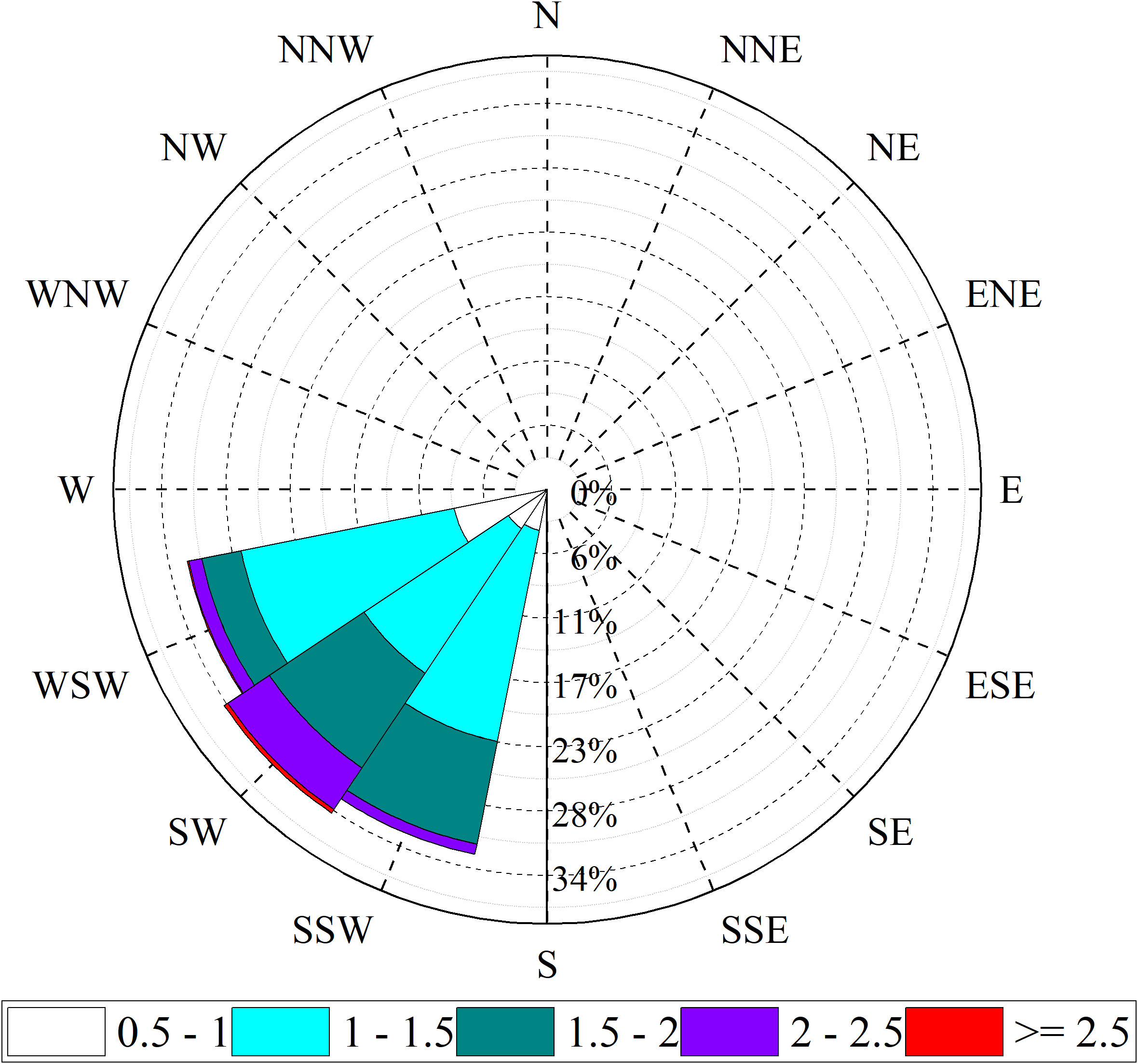
Figure 3. Wave rose diagram relating to significant wave height H_s.

3 Correlation between infragravity waves with sea and swell waves

The wave spectrum integration method (Hwang et al., 2012) was adopted to separate the short-wave components and obtain the dynamic separation frequencies of sea and swell. As shown in Figure 4, the separation frequency obtained using the wave spectrum integration method was relatively stable and lower than the fixed separation frequencies, with an average value of 0.102 Hz.

Figure 4

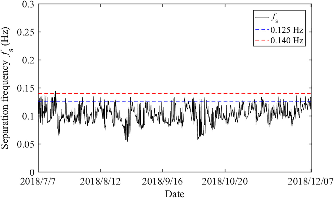
Figure 4. Separation frequency based on wave spectrum integration function.

The separation frequencies obtained using the wave spectrum integration method were compared with two fixed separation frequencies (0.125 and 0.14 Hz), and their effect on the correlation between IGWs and sea and swell waves was analyzed. The wave spectra at representative moments were selected, and the separation effects obtained using the fixed and dynamic separation frequencies are shown in Figure 5. It can be observed that, from the perspective of wave spectral shape, the separation frequencies obtained by the wave spectrum integration method more accurately identify the boundary between the two wave systems.

Figure 5

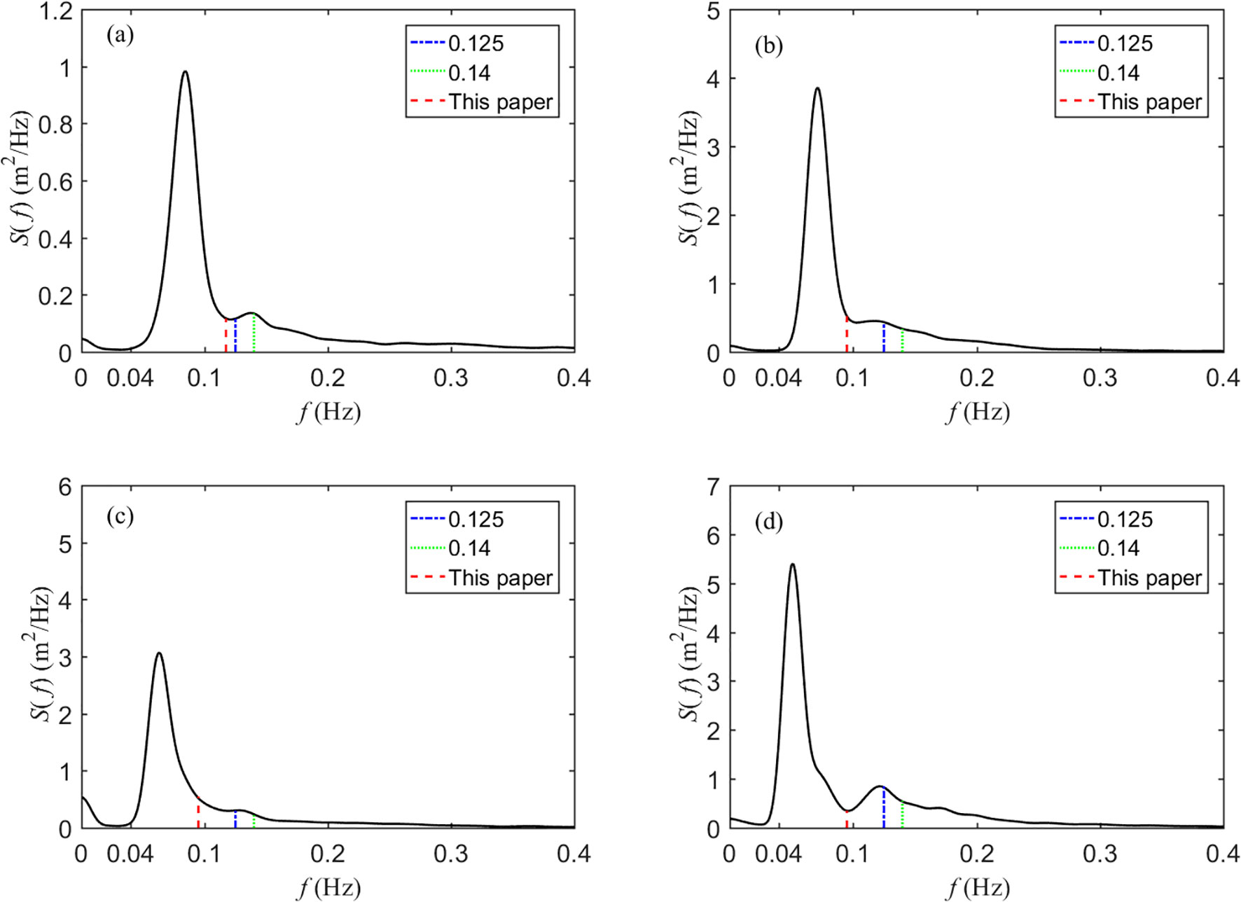
Figure 5. Separation frequencies obtained by different methods (a) 4:00 on July 17, 2018; (b) 9:00 on July 17, 2018; (c) 6:00 on September 20, 2018; and (d) 12:00 on October 18, 2018.

Equation 17 was used to fit the relationship between the IGWs and sea and swell waves, where the coefficient m represented the degree of dependency of IGWs energy on sea and swell energy:

$\begin{array}{ll}{E}_{\text{IGWs}}\propto E_{\text{sea}/\text{swell}}^m& (17)\end{array}$

The energy relationship between the IGWs and sea and swell waves obtained at various separation frequencies is shown in Figure 6. It can be observed that the correlation between IGWs and swell waves was significantly stronger than that with sea waves.

Figure 6

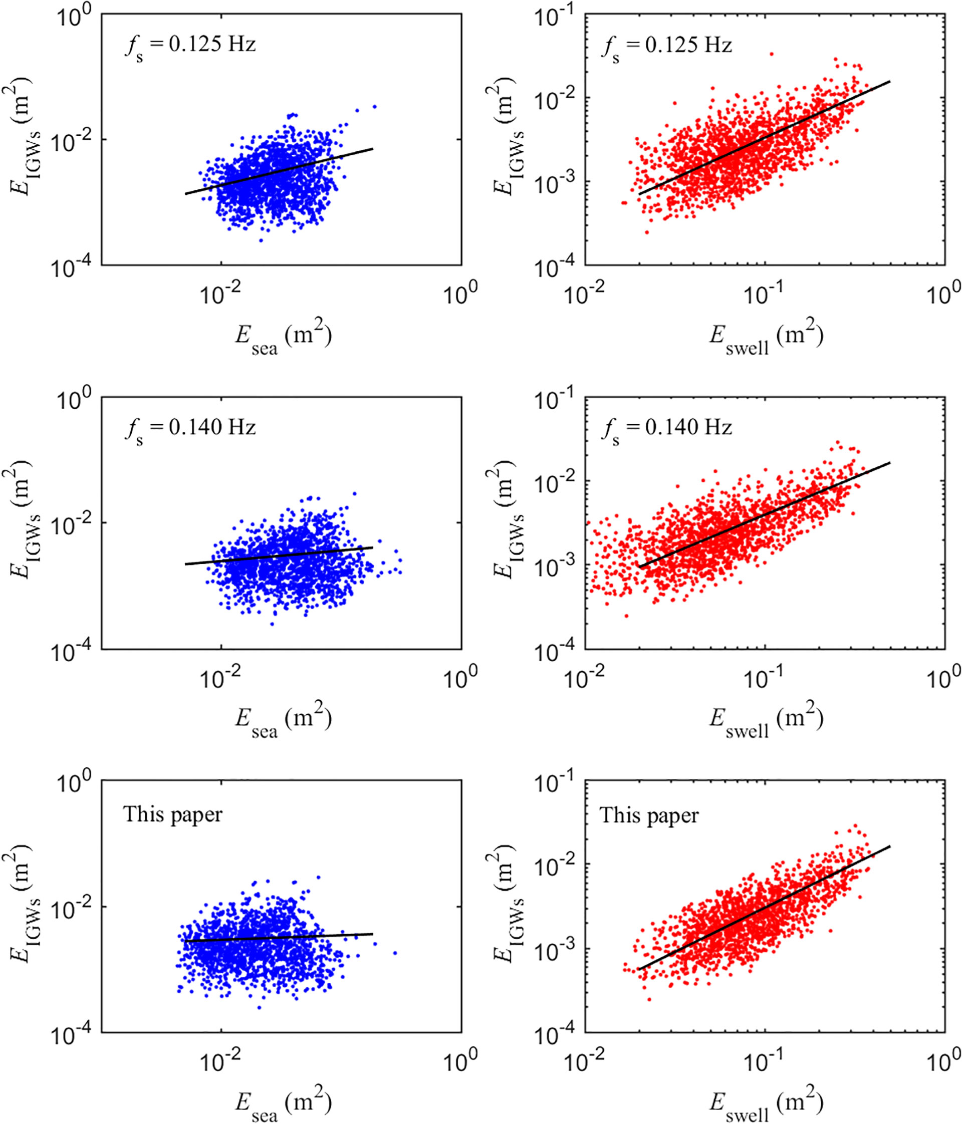
Figure 6. Correlation of IGWs with sea and swell for separation frequencies of 0.125, 0.14 Hz, and based on the wave spectrum integration method.

The correlation coefficient P and the fitting curve coefficient m between the energy of the IGWs and the swell and sea waves were listed in Table 2. The correlation coefficient for swell using the separation frequency calculated by the wave spectrum integration method was the largest, reaching 0.823. Given the performance of the wave spectral shape (Figure 5), the separation frequency obtained by the wave spectrum integration method can be considered more reasonable. This method was adopted to separate sea and swell waves in the subsequent analysis. The coefficient m of the fitting curve was approximately 1.0, indicating a linear correlation between the energy of the IGWs and swell waves.

Table 2

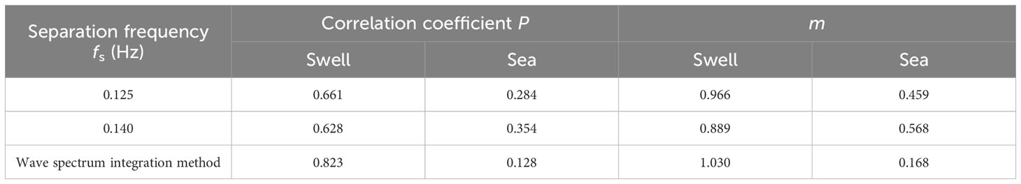
Table 2. The IGWs dependency on swell and sea based on different separation frequencies.

4 Component separation of infragravity waves

According to the research presented in the previous section, the total energy of the IGWs was closely related to the swell waves. Nevertheless, the energy of the observed IGWs was not limited to incident IGWs, but also included free IGWs that were reflected from the shoreline. A sizable amount of energy was accounted for by this portion (Sheremet et al., 2002). As the waves propagated toward the shore, the water depth gradually became shallower, and the energy proportion of the BIG gradually increased. When the short-wave group broke, the BIG was released, and the ratio of BIG energy decreased. Based on field observation data, Ruessink (1998b) found that the ratio of BIG to total IGWs was at a maximum at the breakpoint, where the ratio of short-wave group wave height H_s to the water depth h reached 0.33, and then decreased with larger values of the relative wave height (H_s / h). The ratio of short-wave group wave height H_s to the water depth h at the observation points was shown in Figure 7 and ranged between 0 and 0.2. This indicated that the observation locations were outside the breaking wave zone. Therefore, the FIG was relatively simple in composition, consisting entirely of incident FIG from the open sea, excluding the shoreward FIG caused by short-wave breaking in the breaking wave zone (Baldock et al., 2000). The total IGWs consisted of three parts: incident BIG, incident free infragravity waves (IFIG) and reflected free infragravity waves (RFIG), which facilitated subsequent analysis and energy evaluation of IGWs.

Figure 7

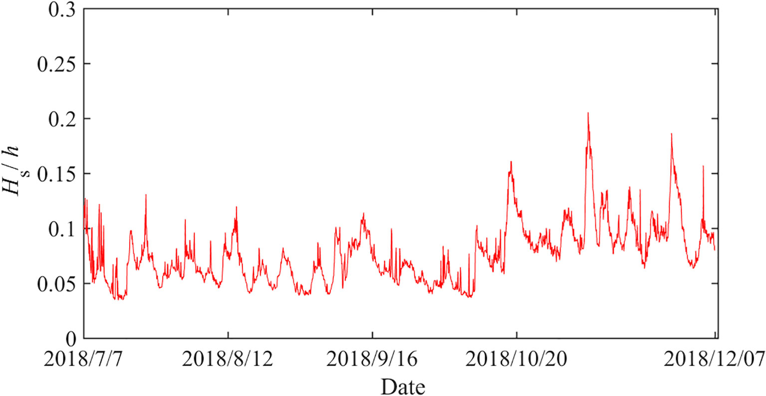
Figure 7. Ratio of short-wave heights to water depth at the observation position.

The cross-correlation spectrum of the wave surface and velocity can be obtained from the Fourier transform of the cross-correlation function. Based on Equations 14, 15, 16, the reflection coefficients of the IGWs at the observation position can be obtained, as shown in Figure 8. The reflection coefficients were mainly distributed between 0.2 and 1.0, which is consistent with the main distribution interval of the reflection coefficients of IGWs in the cross-shore direction obtained in previous research (Sheremet et al., 2002).

Figure 8

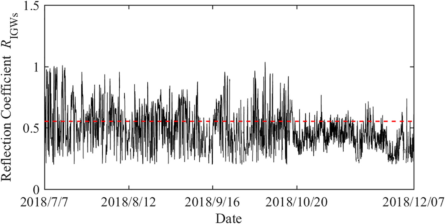
Figure 8. Reflection coefficients RIGWs of infragravity waves.

In the process of wave propagation toward shore, there was strong nonlinear coupling between the BIG and the short-wave group in the shallow region before breaking, resulting in an increase in the IGWs energy flux; that is, the BIG reached its maximum at the breaking point. In the breaking zone, the IGWs flux was reduced owing to the weakened nonlinear coupling and higher dissipation. In the offshore direction, the IGWs were reflected at the coastline and propagated seaward, and the coupling between the reflected IGWs and the short-wave group was weak. The energy of the seaward IGWs decreased with increasing distance from the coastline owing to a combination of deepening effects and dissipation within the breaking zone. However, the spatial variation of the energy flux of the IGWs was smaller in the offshore direction than in the onshore direction, so the reflection coefficient of IGWs even exceeded 1.0 (Sheremet et al., 2002). Under the comprehensive influence of these factors, the reflection coefficient of the IGWs was smallest at the breaking point and increased with the distance from the breaking zone.

It can be seen from the above that the observation location was outside the breaking zone, and the total infragravity waves consisted of incident bound infragravuty wave (BIG), incident free infragravity wave (IFIG) and reflected free infragravity wave (RFIG). Therefore, the total infragravity wave height and reflection coefficient can be expressed as Equations 18, 19:

$\begin{array}{ll}{H}_{\text{IGWs}}=\sqrt{H_{\text{BIG}}^2+H_{\text{FIG}}^2}& (18)\end{array}$

$\begin{array}{ll}{R}_{\text{IGWs}}=\frac{H_{\text{RFIG}}}{\sqrt{H^2{}_{\text{BIG}}+H^2{}_{\text{IFIG}}}}& (19)\end{array}$

Using the above expressions, the wave heights of the BIG, IFIG, and RFIG can be obtained, as shown in Figure 9. It is evident that the wave height of the three IGWs components are comparable in the observed sea. Typically, IFIG is small and can be ignored. However, recent studies have found that a significant number of swells radiate during strong storms, leading to the generation of a non-negligible IFIG. Its magnitude is comparable to or even larger than that of the BIG at medium water depths (Matsuba et al., 2022; Rijnsdorp et al., 2021). No storms occurred during the observation period in this sea area; however, under the influence of the Roaring Forties, long-period swells and IGWs occur throughout the year in this sea area, resulting in a non-negligible IFIG.

Figure 9

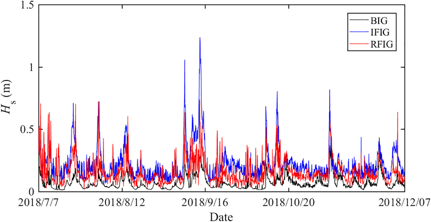
Figure 9. Wave heights of each IGWs component.

5 Energy evaluation of infragravity waves

IGWs have a wide range of applications in nearshore hydrodynamics. However, their long periods and small amplitudes make them difficult to observe and analyze. Based on the correlation between IGWs and short waves, researchers have proposed quantitative relationships between the wave characteristics of IGWs and those of short-wave groups to estimate the energy of IGWs using more easily observable short-wave characteristic parameters. In previous studies, the IGW components were not separated, and a general relationship between the total wave height of the IGWs and the characteristic parameters of the short-wave group was obtained (Bowers, 1992; Herbers et al., 1994; Nelson et al., 1988; Okihiro et al., 1992):

$\begin{array}{ll}{H}_{\text{IGWs}}=K·H_{\text{s}}^{\alpha }{T}_{\text{p}}^{\beta }& (20)\end{array}$

where H_s and T_p are the significant wave height and spectral peak period of short waves; K, α, and β are empirical constants.

The empirical constant varied widely, as shown in Table 3. No unified and clear conclusion has been reached. It is believed that the complex components of the short-wave group and IGWs were not separated during the analysis process, which led to significant differences in the empirical constants.

Table 3

Table 3. Results for empirical constants K, α and β in various literatures.

Based on the above correlation study and wave component separation results, it can be concluded that the correlation between IGWs and swells is stronger than that between IGWs and sea waves, and that the observed IGW components are complex, with each component occupying a significant proportion. Therefore, the wave height of the swell was used to evaluate the energy of the IGWs, and the energies of each IGW component were evaluated separately. The BIG is a second-order wave generated by the nonlinear interaction of the short-wave group, which propagates with the same phase velocity as the short-wave group. There is a strong correlation between the wave height of BIG and the short-wave group. To simplify the expression, only the relationship between the BIG and the swell wave height was considered, leading to the simplified expression Equation 21:

$\begin{array}{ll}{H}_{\text{BIG}}=K·H_{\text{swell}}^{\alpha }& (21)\end{array}$

This expression was adopted to fit the relationship between the wave heights of the BIG and the swell, and the coefficient of determination R² (see Equation 22) was used to evaluate the fitting effect. The fitting results are shown in Figure 10. It was found that the water depth had a significant effect on the wave height of the BIG, which increased significantly due to the shallowing effect. The coefficient of determination R² of the fitting curve exceeded 0.8, indicating that the fitting curve could describe the changes on the measured data effectively. The fitting coefficients are listed in Table 4. The coefficient α related to the wave height was approximately 2.0, indicating an obvious quadratic relationship between the BIG wave height and the swell wave. Additionally, the ratio of the coefficient K at the two observation locations was approximately 0.548, which is approximately inversely proportional to the water depth. This supports the conclusion proposed by Liao et al. (2021) that the growth rate of BIG on slope topography is proportional to h^-1.

Figure 10

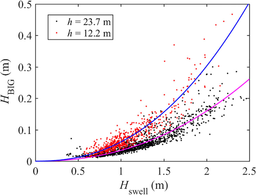
Figure 10. Fitted curves for the variation of BIG wave heights with swell wave heights.

Table 4

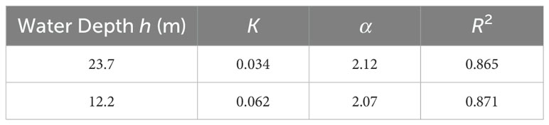
Table 4. Fitting results for the empirical constants K and α in the expression of the BIG wave heights.

$\begin{array}{ll}{R}^2=\frac{{\displaystyle \sum _{i=1}^N{(f(x_i)-\overline{y_i})}^2}}{{\displaystyle \sum _{i=1}^N{(y_i-\overline{y_i})}^2}}& (22)\end{array}$

The FIG, includes both incident free infragravity waves (IFIG) and reflected free infragravity waves (RFIG). Equation 20 was used to fit the measured FIG wave heights, using swell wave heights. A comparison of the measured and fitted IFIG and RFIG values is shown in Figure 11. For the IFIG, the fitting results follow the overall trend of wave height variation, and the coefficient of determination R² of the fitting curve exceeded 0.8, the fitting results represent the measured wave heights well. For the RFIG, the coefficient of determination coefficient R² was relatively small especially in conditions of high wave heights. It indicated that there was no significant correlation between the RFIG and the swell wave heights. In summary, the correlation between the FIG and swell waves was weaker than that between of the BIG and swell waves.

Figure 11

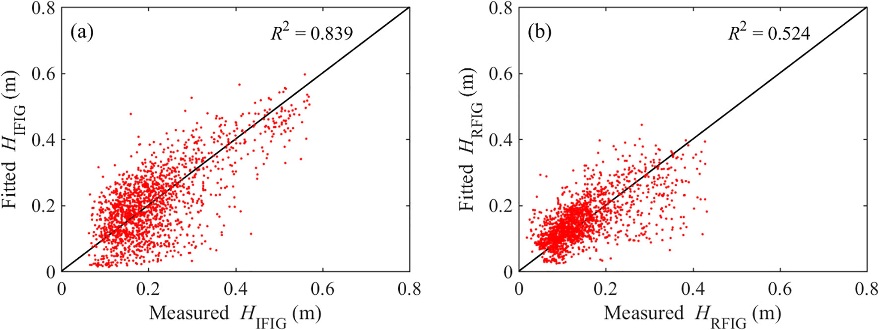
Figure 11. Comparisons of fitted and measured FIG wave heights (a) IFIG, and (b) RFIG.

In practical ocean engineering, more attention has been paid to the correlation between the total incident IGWs and the short-wave group. It is expected that the wave height of the incident IGWs can be calculated using the wave characteristic parameters of the short-wave group. The wave height of the total incident IGWs (IIG) is calculated as Equation 23:

$\begin{array}{ll}{H}_{\text{IIG}}=\sqrt{H^2{}_{\text{BIG}}+H^2{}_{\text{IFIG}}}& (23)\end{array}$

Equation 20 was used to fit the IIG wave heights, and the results are shown in Figure 12. The coefficient of determination R² of the fitting curve exceeded 0.8, and the fitting effect was significantly improved compared to that of the FIG. Under the influence of the IFIG and the introduction of the spectral peak period T_p, the coefficient α related to the wave height was approximately 1.0.

Figure 12

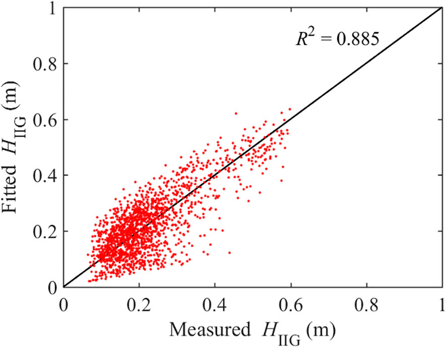
Figure 12. Comparisons of fitted and measured IIG wave heights.

6 Conclusions

The characteristics of IGWs were studied based on field observations. The correlation between IGWs and short waves was analyzed, and the energy of the IGWs was evaluated. The following conclusions were drawn:

The effects of different sea and swell wave separation methods were also studied. The separation frequency obtained using the wave spectrum integration method was relatively stable and lower than the fixed separation frequencies (0.125 and 0.14 Hz). By comparing the performance of the separation frequency in terms of the wave spectral shape and the correlation between the IGWs and short waves, it was concluded that the separation frequency obtained using the spectral integral method was more reasonable. The correlation between IGWs and swell waves was significantly stronger than that with sea waves.

The wave height of the BIG was obtained based on second-order nonlinear theory, and the spectral domain separation method was used to separate the incident and reflected IGWs. The separation of the various components of the IGWs was achieved using the above methods. Under the influence of the Roaring Forties, the wave height proportions of the three IGW components (BIG, IFIG, and RFIG) were comparable in the observed sea, and IFIG was non-negligible.

Based on the separation results for short waves and IGWs, the characteristic parameters of swell were adopted to evaluate the energy of the IGWs. For the BIG, there was a significant quadratic relationship between the wave heights of the BIG and the swell waves. The correlation between the FIG and swell waves was weaker than that between the BIG and swell waves. For the total incident IGWs, the empirical expression between the wave height of the IIG and the characteristic parameters of swell was obtained, and the coefficient α related to wave height was approximately 1.0.

The wave spectrum integration method was adopted for sea and swell wave separation, and the quantitative relationship between IGWs and short-wave characteristic parameters was obtained. The limitation of this separation method was that it lacked a certain physical foundation, further collections of field measurements were required for verification or correction in the future.

Data availability statement

The original contributions presented in the study are included in the article/supplementary material. Further inquiries can be directed to the corresponding author.

Author contributions

XG: Data curation, Formal analysis, Resources, Writing – original draft, Writing – review & editing. ZH: Investigation, Methodology, Writing – review & editing. JJ: Funding acquisition, Project administration, Writing – review & editing. YJ: Resources, Supervision, Writing – review & editing.

Funding

The author(s) declare that financial support was received for the research and/or publication of this article. This study was financially supported by the Postdoctoral Science Foundation (Grant No. P66525) and a self-supporting research project (Grant No. P48521) of Power China Chengdu Engineering Corporation Limited.

Conflict of interest

Authors XG, ZH, JJ and YJ were employed by the company PowerChina Chengdu Engineering Corporation Limited.

The authors declare that this study received funding from PowerChina Chengdu Engineering Corporation Limited. The funder had the following involvement in the study: the study design and preparation of the manuscript.

Generative AI statement

The author(s) declare that no Generative AI was used in the creation of this manuscript.

Publisher’s note

All claims expressed in this article are solely those of the authors and do not necessarily represent those of their affiliated organizations, or those of the publisher, the editors and the reviewers. Any product that may be evaluated in this article, or claim that may be made by its manufacturer, is not guaranteed or endorsed by the publisher.

References

Almar R., Michallet H., Cienfuegos R., Bonneton P., Tissier M., and Ruessink G. (2014). On the use of the Radon Transform in studying nearshore wave dynamics. Coast. Eng. 92, 24–30. doi: 10.1016/j.coastaleng.2014.06.008

Crossref Full Text | Google Scholar

Ardhuin F., Rawat A., and Aucan J. (2014). A numerical model for free infragravity waves: Definition and validation at regional and global scales. Ocean Model. 77, 20–32. doi: 10.1016/j.ocemod.2014.02.006

Crossref Full Text | Google Scholar

Baldock T. E., Huntley D. A., Bird P. A. D., O’Hare T., and Bullock G. N. (2000). Breakpoint generated surf beat induced by bichromatic wave groups. Coast. Eng. 39, 213–242. doi: 10.1016/S0378-3839(99)00061-7

Crossref Full Text | Google Scholar

Bertin X., de Bakker A., van Dongeren A., Coco G., André G., and Ardhuin F. (2018). Infragravity waves: From driving mechanisms to impacts. Earth-Science Rev. 177, 774–799. doi: 10.1016/j.earscirev.2018.01.002

Crossref Full Text | Google Scholar

Bowers E. C. (1992). Low frequency waves in intermediate water depths. 23rd Int. Conf. Coast. Eng. 832–845. 10.1061/9780872629332.062

Google Scholar

De Bakker A. T. M., Tissier M. F. S., and Ruessink B. G. (2014). Shoreline dissipation of infragravity waves. Continental Shelf Res. 72, 73–82. doi: 10.1016/j.csr.2013.11.013

Crossref Full Text | Google Scholar

Dolenc D., Romanowicz B., McGill P., and Wilcock W. (2008). Observations of infragravity waves at the ocean-bottom broadband seismic stations Endeavour (KEBB) and Explorer (KXBB). Geochemistry Geophysics Geosystems 9, 1–18. doi: 10.1029/2008gc001942

Crossref Full Text | Google Scholar

Dolenc D., Romanowicz B., Stakes D., McGill P., and Neuhauser D. (2005). Observations of infragravity waves at the Monterey ocean bottom broadband station (MOBB). Geochemistry Geophysics Geosystems 6, 1–13. doi: 10.1029/2005gc000988

Crossref Full Text | Google Scholar

Dong G., Guo L., Zheng Z., and Ma X. (2024). Observations of coastal infragravity wave characteristics under swell-dominated conditions. Appl. Ocean Res. 148, 1–17. doi: 10.1016/j.apor.2024.104032

Crossref Full Text | Google Scholar

Dong G., Zheng Z., Ma X., and Huang X. (2020). Characteristics of low-frequency oscillations in the Hambantota Port during the southwest monsoon. Ocean Eng. 208, 1–10. doi: 10.1016/j.oceaneng.2020.107408

Crossref Full Text | Google Scholar

Earle M. D. (1984). Development of algorithms for separation of sea and swell [R]. National Data Buoy Center Tech Rep MEC-87-1, NDBC, 53, 1–15.

Google Scholar

Elgar S., Herbers T. H. C., Okihiro M., Oltman-Shay J., and Guza R. T. (1992). Observations of infragravity waves. J. Geophysical Res. 97, 573–577. doi: 10.1029/92jc01316

Crossref Full Text | Google Scholar

Gao J., Hou L., Liu Y., and Shi H. (2024). Influences of bragg reflection on harbor resonance triggered by irregular wave groups. Ocean Eng. 305, 1–22. doi: 10.1016/j.oceaneng.2024.117941

Crossref Full Text | Google Scholar

Gao J., Ma X., Dong G., Chen H., Liu Q., and Zang J. (2021). Investigation on the effects of Bragg reflection on harbor oscillations. Coast. Eng. 170, 1–17. doi: 10.1016/j.coastaleng.2021.103977

Crossref Full Text | Google Scholar

Gao J., Ma X., Zang J., Dong G., Ma X., Zhu Y., et al. (2020). Numerical investigation of harbor oscillations induced by focused transient wave groups. Coast. Eng. 158, 1–17. doi: 10.1016/j.coastaleng.2020.103670

Crossref Full Text | Google Scholar

Gao J., Shi H., Zang J., and Liu Y. (2023). Mechanism analysis on the mitigation of harbor resonance by periodic undulating topography. Ocean Eng. 281, 1–19. doi: 10.1016/j.oceaneng.2023.114923

Crossref Full Text | Google Scholar

Gao J., Zhou X., Zhou L., Zang J., and Chen H. (2019). Numerical investigation on effects of fringing reefs on low-frequency oscillations within a harbor. Ocean Eng. 172, 86–95. doi: 10.1016/j.oceaneng.2018.11.048

Crossref Full Text | Google Scholar

Godin O. A., Zabotin N. A., Sheehan A. F., Yang Z., and Collins J. A. (2013). Power spectra of infragravity waves in a deep ocean. Geophysical Res. Lett. 40, 2159–2165. doi: 10.1002/grl.50418

Crossref Full Text | Google Scholar

Guza R. T., Thornton E. B., and Holman R. A. (1984). Swash on steep and shallow beaches. 19th Int. Conf. Coast. Eng., 708–723. doi: 10.1061/9780872624382.049

Crossref Full Text | Google Scholar

Hasselmann K. (1962). On the non-linear energy transfer in a gravity wave spectrum part 1. General theory. J. Fluid Mechanics 12, 481–500. doi: 10.1017/S0022112062000373

Crossref Full Text | Google Scholar

Herbers T. H. C., Elgar S., and Guza R. T. (1994). Infragravity-frequency (0.005–0.05 hz) motions on the shelf. Part I:Forced waves. J. Phys. Oceanography 24, 917–927. doi: 10.1175/1520-0485(1994)024<0917:IFHMOT>2.0.CO;2

Crossref Full Text | Google Scholar

Holman R. A. and Bowen A. J. (1982). Bars, bumps, and holes: Models for the generation of complex beach topography. J. Geophysical Res. 87, 457–468. doi: 10.1029/JC087iC01p00457

Crossref Full Text | Google Scholar

Holthuijsen L. H. (2007). Waves in Oceanic and Coastal Waters (New York: Cambridge University Press).

Google Scholar

Hwang P. A., Ocampo-Torres F. J., and García-Nava H. (2012). Wind sea and swell separation of 1D wave spectrum by a spectrum integration method. J. Atmospheric Oceanic Technol. 29, 116–128. doi: 10.1175/jtech-d-11-00075.1

Crossref Full Text | Google Scholar

Lara J. L., Martin F. L., and Losada I. J. (2002). Experimental analysis of long waves at the mouth of Gijon harbor. Water Eng. 9, 437–451. doi: 10.1142/9789812701916_0104

Crossref Full Text | Google Scholar

Li S., Liao Z., Liu Y., and Zou Q. (2020). Evolution of infragravity waves over a shoal under nonbreaking conditions. J. Geophysical Research: Oceans 125, 1–15. doi: 10.1029/2019jc015864

Crossref Full Text | Google Scholar

Liao Z., Li S., Liu Y., and Zou Q. (2021). An Analytical Spectral Model for Infragravity Waves over Topography in Intermediate and Shallow Water under Nonbreaking Conditions. J. Phys. Oceanography 51, 2749–2765. doi: 10.1175/jpo-d-20-0164.1

Crossref Full Text | Google Scholar

Mahmoudof S. M. (2018). Investigation of infragravity waves dependency on wind waves for breaking and nonbreaking conditions in the sandy beaches of Southern Caspian Sea (Nowshahr Port). Int. J. Coast. offshore Eng. 1, 13–20. doi: 10.29252/ijcoe.1.4.13

Crossref Full Text | Google Scholar

Mahmoudof S. M. and Siadatmousavi S. M. (2020). Bound infragravity wave observations at the Nowshahr beaches, southern Caspian Sea. Appl. Ocean Res. 98, 1–13. doi: 10.1016/j.apor.2020.102122

Crossref Full Text | Google Scholar

Mahmoudof S. M. and Takami M. L. (2022). Numerical study of coastal wave profiles at the sandy beaches of Nowshahr (Southern Caspian Sea). Oceanologia 64, 457–472. doi: 10.1016/j.oceano.2022.03.001

Crossref Full Text | Google Scholar

Matsuba Y., Roelvink D., Reniers A. J. H. M., Rijnsdorp D. P., and Shimozono T. (2022). Reconstruction of directional spectra of infragravity waves. J. Geophysical Research: Oceans 127, 1–20. doi: 10.1029/2021jc018273

Crossref Full Text | Google Scholar

Matsuba Y., Shimozono T., and Sato S. (2020). Infragravity wave dynamics on Seisho Coast during Typhoon Lan in 2017. Coast. Eng. J. 62, 299–316. doi: 10.1080/21664250.2020.1753901

Crossref Full Text | Google Scholar

Matsuba Y., Shimozono T., and Tajima Y. (2021). Extreme wave runup at the Seisho Coast during Typhoons Faxai and Hagibis in 2019. Coast. Eng. 168, 1–14. doi: 10.1016/j.coastaleng.2021.103899

Crossref Full Text | Google Scholar

Medina J. R. (1990). The dependency of inshore long waves on the characteristics of offshore short waves. Coast. Eng. 14, 185–190. doi: 10.1016/0378-3839(90)90017-Q

Crossref Full Text | Google Scholar

Mendes D., Fortunato A. B., Bertin X., Martins K., Lavaud L., Nobre Silva A., et al. (2020). Importance of infragravity waves in a wave-dominated inlet under storm conditions. Continental Shelf Res. 192, 1–15. doi: 10.1016/j.csr.2019.104026

Crossref Full Text | Google Scholar

Nagai T., Hashimoto N., Asai T., Tobiki I., lto K., Toue T., et al. (1994). “Relationship of a moored vessel in a habor and a long wave caused by wave groups,” Paper presented at the Proceedings of 24th International Conference on Coastal Engineering, 847–860. doi: 10.1061/9780784400890.063

Crossref Full Text | Google Scholar

Nelson R. C., Treloar P. D., and Lawson N. V. (1988). The dependency of inshore long waves on the characteristics of offshore short waves. CoastalEngineering 12, 213–231. doi: 10.1016/0378-3839(88)90006-3

Crossref Full Text | Google Scholar

Okihiro M., Guza R. T., and Seymour R. J. (1992). Bound infragravity waves. J. Geophysical Research: Oceans 97, 11453–11469. doi: 10.1029/92jc00270

Crossref Full Text | Google Scholar

Prevosto M., Ewans K., Forristall G. Z., and Olagnon M. (2013). “Swell genesis, modelling and measurements in West Africa,” in Proceedings of the ASME 2013 32nd International Conference on Ocean, Offshore and Arctic Engineering (OMAE2013), 1–12. doi: 10.1115/OMAE2013-11201

Crossref Full Text | Google Scholar

Rijnsdorp D. P., Reniers A. J. H. M., and Zijlema M. (2021). Free infragravity waves in the North Sea. J. Geophysical Research: Oceans 126, 1–14. doi: 10.1029/2021jc017368

Crossref Full Text | Google Scholar

Roeber V. and Bricker J. D. (2015). Destructive tsunami-like wave generated by surf beat over a coral reef during Typhoon Haiyan. Nat. Commun. 6, 1–10. doi: 10.1038/ncomms8854

PubMed Abstract | Crossref Full Text | Google Scholar

Ruessink B. G. (1998a). Bound and free infragravity waves in the nearshore zone under breaking and nonbreaking conditions. J. Geophysical Research: Oceans 103, 12795–12805. doi: 10.1029/98jc00893

Crossref Full Text | Google Scholar

Ruessink B. G. (1998b). The temporal and spatial variability of infragravity energy in a barred nearshore zone. Continental Shelf Res. 18, 585–605. doi: 10.1016/S0278-4343(97)00055-1

Crossref Full Text | Google Scholar

Sheremet A., Guza R. T., Elgar S., and Herbers T. H. C. (2002). Observations of nearshore infragravity waves: Seaward and shoreward propagating components. J. Geophysical Res. 107, 1–10. doi: 10.1029/2001jc000970

Crossref Full Text | Google Scholar

Smith G. G. and Mocke G. P. (2002). Interaction between breaking broken waves and infragravity-scale phenomena to control sediment suspension transport in the surf zone. Mar. Geology 187, 329–345. doi: 10.1016/S0025-3227(02)00385-7

Crossref Full Text | Google Scholar

Sugioka H., Fukao Y., and Kanazawa T. (2010). Evidence for infragravity wave-tide resonance in deep oceans. Nat. Commun. 1, 1–7. doi: 10.1038/ncomms1083

PubMed Abstract | Crossref Full Text | Google Scholar

Van Dongeren A., Battjes J., Janssen T., van Noorloos J., Steenhauer K., Steenbergen G., et al. (2007). Shoaling and shoreline dissipation of low-frequency waves. J. Geophysical Res. 112, 1–15. doi: 10.1029/2006jc003701

Crossref Full Text | Google Scholar

Vis F. C. A., Mol M. M., and Rita C. D. (1985). “Long waves and harbor design,” in Paper presented at the Int. Conf. on Num. & Hyd. Modelling of ports and harbors (Key West, Florida, USA: IAHR and BHRA).

Google Scholar

Wang D. W. and Hwang P. A. (2001). An operational method for separating wind sea and swell from ocean wave spectra. J. Atmospheric Oceanic Technol. 18, 2052–2062. doi: 10.1175/1520-0426(2001)018<2052:Aomfsw>2.0.Co;2

Crossref Full Text | Google Scholar

Zheng Z., Ma X., Ma Y., Huang X., and Dong G. (2021). Modeling of coastal infragravity waves using the spectral model WAVEWATCH III. Coast. Eng. 170, 1–14. doi: 10.1016/j.coastaleng.2021.104016

Crossref Full Text | Google Scholar