Characteristics and distribution of surface sediments in the Central East China Sea shelf

Based on grain-size analysis of the surface sediments on the central East China Sea (ECS) shelf, the spatial distribution, depositional settings, and transport patterns of these sediments were investigated in 2022. The results show that the study area can be divided into four Subareas: the nearshore clayey-silt or silt-dominated muddy deposition Subarea (Subarea I), the inner shelf silty-clay-dominated muddy deposition Subarea (Subarea II), the inner and outer shelf transition zone sand-silt-clay or clayey-sand-dominated mixed deposition Subarea (Subarea III), and the outer shelf sandy deposition Subarea (Subarea IV). Typical sediment grain size frequency curves and cumulative frequency curves reflect the sediment differentiation in Subareas I and II, as well as the sediment mixing and modification in Subareas III and IV. The spatial distribution of the sediments is affected by the hydrodynamic and environmental conditions. The main components of the surface sediments in this area are Yangtze River-derived terrigenous clasts. The contents of the sand, silt, and clay fractions obtained using the laser grain size analysis method were approximately 5% larger, 20% larger, and 25% smaller, respectively, than those acquired using the sieve and pipette analysis method, which was the reason that clayey-silt has been reported to occupy almost all of the muddy zone (Subareas I and II) in previous studies. Grain-size trend analysis images revealed the existence of generally north-to-south and west-to-east (i.e., coast-to-offshore) transport trends of the surface sediment in this area, indicating continuity of the provenance, environment, age, and genetic type of the sediments on the ECS shelf. Local regions exhibited different transport directions, which were influenced by the northward Taiwan Warm Current and upwelling. Mixed sediments experienced material redistribution and exchange with neighboring muddy and sandy deposits. The bidirectional northwest-southeast transport trends of some sandy sediments suggest a tidal genesis of the linear sand ridges and their effect on the sandy sediments in this region. Fine clay particles are spread over the entire ECS shelf, suggesting cross-shelf transport of modern fine-grained sediments.

1 Introduction

Characteristics, spatial distribution, and transport pattern of marine sediments contain abundant geological and environmental information (Nittrouer et al., 1984; Milliman et al., 1989; Lantzsch et al., 2014). In particular, the sediments in continental margins, where strong sea-land interactions and high sedimentation rates occur, are important records for studying the global biogeochemical cycle, climate change, and anthropogenic effects. Therefore, delineating their sedimentation natures and spatial distributions, and transport patterns is of great importance for both scientific research and practical applications (Le Roux et al., 2002; Dong et al., 2011; Zhang et al., 2020; Liang et al., 2020).

The central East China Sea (ECS) shelf area possesses representative significance due to its rich surface sediment types, and as a result making it the main part of the ECS marine deposit (Figure 1). In addition, it hosts a full spectrum of surface-sediment facies, mud, mixed sand–mud, and relict sand and it lies at the confluence of strong tidal currents, seasonally reversing monsoon winds, and multiple fluvial inputs. Topographically, the terrain in the study area decreases gently toward the southeast and can be divided into the inner shelf and outer shelf by a water depth of 50–60 m. The sediments are spread along the shoreline in the form of strips (Qin et al., 1987; Xu et al., 1997; Li, 2008). A considerable amount of research has been conducted in this area, and the following consensus has been reached: the upper part of the nearshore and inner shelf is covered by a wedge-shaped muddy zone (Inner Shelf Muddy Belt, ISMB) and the major sediments are silty-clay (TY) or clayey-silt (YT), which are modern deposits mainly composed of terrigenous detritus carried by the Yangtze River dispersal system and transported from north to south alongshore and eastward down into the offshore area (Milliman et al., 1989; Liu et al., 2007a; Xu et al., 2012).

Figure 1

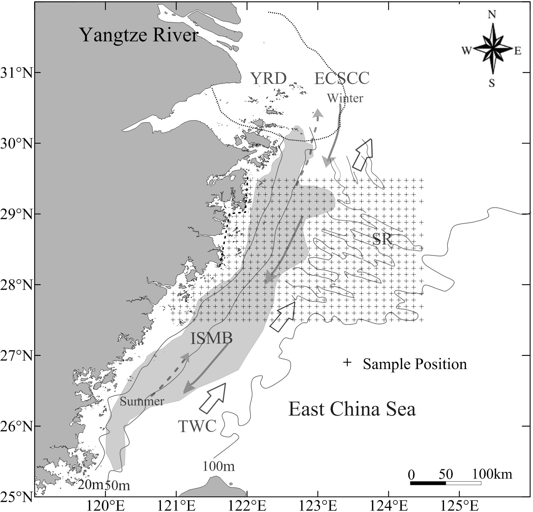
Figure 1. Sampling locations in the study area. Modified from Bao et al. (2005); Zhuang et al. (2005); Liu et al. (2007a), and Wu et al. (2010). YRD, Yangtze River Subaqueous Delta; ISMB, Inner Shelf Mud Belt; ECSCC, East China Sea Coastal Current; TWC, Taiwan Warm Current; and SR, Sand Ridges.

The Inner Shelf Mud Belt (ISMB) refers to a broad zone of fine-grained sediment accumulation located along the inner continental shelf, particularly influenced by fluvial inputs such as those from the Yangtze River. Composed mainly of silts and clays, the ISMB is formed under relatively low-energy hydrodynamic conditions that allow suspended sediments to settle. Its significance lies in its role as a major sediment sink and archive, preserving valuable records of terrestrial input, oceanographic processes, and environmental changes over time. In addition, their grain-size characteristics, spatial distribution, sedimentation rate, and depositional processes are controlled by the circulation system and the tidal and wave regime in the ECS (Huh and Su, 1999; Guo et al., 2002; Liu et al., 2015). The ECS outer shelf deposits are dominated by fine sand (FS). These deposits primarily formed before the Holocene maximum sea level (ca. 7 ka B.P.) and have undergone modification, accompanied by the development of extensive linear sand ridges (SR) (Saito et al., 1998; Berne et al., 2002; Li et al., 2014). The mixed deposits are distributed between the outer shelf sandy deposits and the inner shelf muddy deposits (Xu et al., 1997; Li, 2008), and the main sediment types are sand-silt-clay (S-T-Y) or clayey sand (YS).

In recent years, researchers have gained deeper insights into how sediments move and settle across the East China Sea (ECS) shelf. For instance, Chen et al. (2021) conducted field experiments near the Yangtze River mouth and found that tidal currents near the seabed play a major role in lifting and pushing sediments offshore. Similarly, Wang et al. (2024) used underwater current meters (ADCPs) to measure long-term water movement and observed patterns of flow that change direction seasonally, helping explain how sediments can travel both along the coast and away from it. Cong et al. (2024) showed that strong winter storms resuspend sediments and push fine particles far beyond the nearshore mud zones sometimes over 100 kilometres out to sea. These studies support the idea that sediment transport in the ECS is not constant throughout the year, but instead varies with seasonal winds, tides, and storms.

In addition to field data, other researchers have used modern tools like satellite imagery and computer models to better understand ECS sediment dynamics. Peng and Yin (2025) analysed satellite images and found that surface waters carrying suspended particles are often pushed offshore during the winter monsoon season, confirming earlier field observations. Zhang et al. (2023) used numerical models to simulate how sediments move in response to changing ocean currents and showed that sudden pulses of sediment can occur when coastal water fronts shift. Furthermore, Kaur et al. (2024) highlighted how internal tide waves that move within the ocean rather than on its surface can stir up sediments along the seabed and influence their transport direction. Altogether, these recent findings provide a strong scientific foundation for re-examining how sediments are distributed across the ECS and help explain the patterns identified in this study, such as cross-shelf mixing and sediment reworking in deeper waters.

While the Yangtze River is indeed the dominant sediment source for the central East China Sea (ECS) shelf, accounting for over 85% of the total terrigenous input (Liu et al., 2007a; Zhao et al., 2020), we recognize that other regional sources, such as the Qiantang and Ou rivers, and coastal erosion, also contribute sediments particularly to nearshore and southern Subareas. Recent geochemical studies (e.g., Zhang et al., 2019; Xu et al., 2022) show that sediments from the Qiantang River and Ou River basins have distinct isotopic signatures (higher ^87Sr/^86Sr and more radiogenic ϵNd values) compared to the Yangtze. In particular, Xu et al. (2022) report that Sr-Nd isotopic mixing models estimate contributions of up to 8–12% from these southern rivers in the coastal zones south of 28.5°N. Moreover, coastal erosion in Zhejiang and Fujian provinces, especially in the Hangzhou Bay area, is responsible for delivering fine clastic material with similar mineralogical fingerprints to the adjacent mountainous lithologies (Li et al., 2017). This clarification strengthens the interpretation of spatial heterogeneity in sediment sourcing and is consistent with the stratified distribution of clay-rich fractions in the nearshore zones identified in our grain-size data.

Regarding the type and distribution of the surface sediments in the muddy zone, some earlier studies have divided them into silt (T), YT, and TY, with a distribution pattern of coarse (T or YT), fine (TY) and then coarse (mixed deposits) from the west coastal area eastward toward the offshore area (Xu et al., 1997; Li, 2008; Li and Zhang, 2020). However, in recent studies, the muddy deposits are almost all reported to be YT, while TY is rare (Liu et al., 2009; Liang et al., 2020). These sediment type differences have caused differences in the descriptions and interpretations of the spatial distribution range, grain-size characteristics, and geological and environmental meanings of the sediments (Huang et al., 2014; Wang et al., 2020).

The reported sediment transport patterns in the inner shelf and adjacent areas are also widely divergent. Liu et al. (2009) reported that the main body of the muddy deposit was transported southward by the East China Sea coastal current (ECSCC), and its two sides were transported outward, i.e., westward in the coastal area and eastward in the East Sea area. Other scholars have suggested that the sediment transport direction was related to the strength and direction of the ECSCC and monsoon, generally transporting sediment southward in winter and northward in summer according to the strengthening of the summer winds and the Taiwan Warm Current (TWC) (Bian et al., 2013; Liang et al., 2020). The Taiwan Warm Current (TWC) is a northward-flowing branch of the Kuroshio Current that enters the East China Sea through the Taiwan Strait. It is a warm, saline current that significantly influences the hydrography and sediment dynamics of the continental shelf by enhancing vertical mixing, promoting coastal upwelling, and altering sediment transport pathways. The TWC plays a critical role in redistributing fine-grained sediments offshore and shaping the seasonal and spatial variability of depositional environments in regions like Subareas III and IV. It has also been suggested that the sediments were transported from the periphery to the depositional center (Liu et al., 2007a; Xu et al., 2012). Regarding the cross-shelf transport of modern fine-grained materials from the inner shelf to the deep sea, previous studies have focused on the diffusion extent and mechanism of the suspended sediment (Dong et al., 2011; Liu et al., 2015; Zhang et al., 2019), while seafloor sediments have not yet been sufficiently studied.

Although the sediment types and distribution range of the mixed deposits have been investigated by most scholars (Li, 2008; Li and Zhang, 2020), fewer studies have been conducted on their sediment characteristics, depositional setting, and mixing patterns. The outer shelf sandy sediments are not consistent with the modern hydrodynamic conditions and underwent modification during the period of sea level rise (Emery, 1968; Chen, 1997; Uehara and Saito, 2003). However, studies have mainly focused on the structure and evolution of sand ridges (Berne et al., 2002; Liu et al., 2007b; Wu et al., 2010), and research on the grain size features and transport patterns of the surficial sediments that represent the present state is lacking.

The sedimentary pattern in the ECS was shaped by two types of deposits with different periods and geneses, i.e., patchy or banded modern muddy deposits overlying sandy sediments formed during the low sea level period (Nittrouer et al., 1984; Qin et al., 1987; Li et al., 2014). Moreover, cores drilled in the inner shelf area have revealed the existence of a vertical sediment distribution pattern, i.e., muddy deposits to mixed deposits to sandy deposits from top to bottom, which is analogous to the horizontal pattern from the coast to the offshore area (Li, 2008; Li and Zhang, 2020). These three deposit types of deposits are continuously spread in the central ECS margin, which is approximately 300 km (121–124°E) wide from the western coast to the eastern outer shelf, providing an ideal area for exploring the connection and differences between these three types of deposits.

The scientific problem of this study can be summarized in this way that there is a lack of clarity and consistency in understanding the spatial distribution, textural classification, and transport patterns of surface sediments on the central East China Sea (ECS) shelf due to methodological discrepancies between classical (sieve–pipette) and modern (laser diffraction) grain-size analysis techniques, insufficient spatial resolution of sediment data, and incomplete integration of recent hydrodynamic insights.

Accordingly, we collected 616 surface-sediment samples from March to May 2022 and conducted sediment sampling and analysis with a grid spacing of 10 km from the coast of the study area to the outer shelf (water depth of approximately 110 m) (Figure 1) with the support of the Spatial Resource Investigation Program. In this study, we analyzed the characteristics, spatial distribution, and transport patterns of the surface sediments in the central ECS shelf area. The main objectives of this study were (1) to clarify the types and spatial distribution of the surface sediments in the study area; (2) to quantify and reconcile the methodological differences between SPM and LPM, and thereby resolving the controversy in research on the muddy deposits caused by the use of different grain-size analysis methods; and (3) to delineate the sediment transport pattern and influencing factors in the study area and to explore the geological and environmental significance of the surface sediments in the study area by combining their grain size, distribution, and transport characteristics. This study directly addresses these issues by applying both SPM and LPM to a dense dataset of 616 samples, utilizing a stratified-random sampling design to ensure spatial and environmental representativeness. It interprets sediment transport patterns using grain-size trend analysis, complemented by recent oceanographic and geochemical studies.

2 Materials and methods

Immediately after recovery, Samples of the uppermost surficial (0–1 cm) layer of the surface sediments were collected with a Teflon spatula using a box sampler, placed in acid-washed polypropylene jars, and kept at 4 degrees Celsius at a total of 616 sampling stations (Figure 2). In the laboratory the material was oven-dried at 40°C to constant weight, lightly disaggregated with a rubber pestle, and quarter-split to obtain a representative 10 g aliquot. To remove carbonate shell fragments, the bulk sample was wet-sieved through a 2 mm screen; coarse bioclasts were discarded.

Figure 2

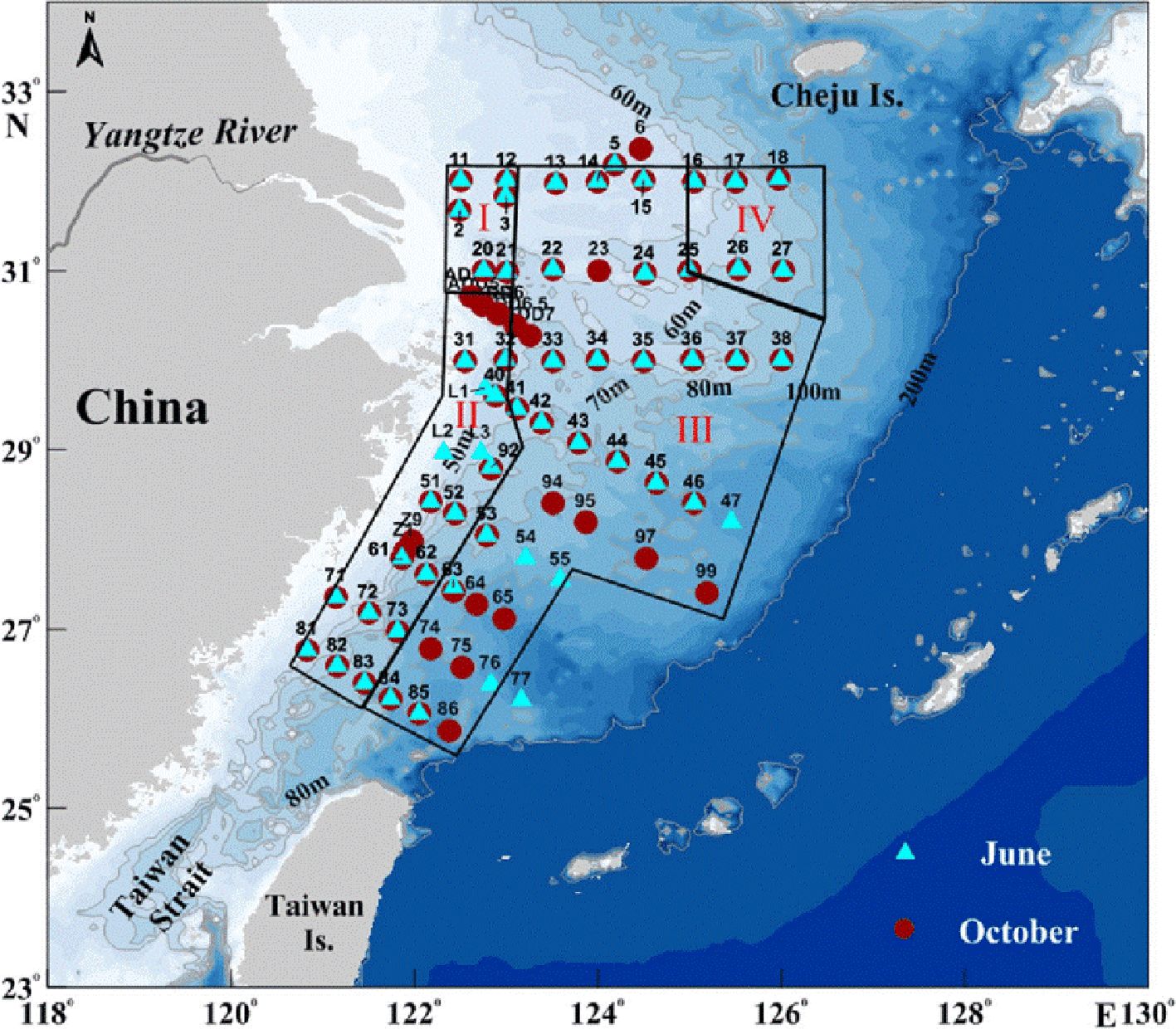
Figure 2. Sediments’ sampling zones.

Prior to grain-size measurement, sediment samples were subjected to a standardized pretreatment protocol to remove confounding components and ensure uniform particle dispersion. Approximately 5 g of air-dried sediment from each sample was first sieved through a 2 mm mesh to remove coarse debris and homogenize the subsample. To eliminate organic matter, samples were treated with 10 mL of 30% hydrogen peroxide (H₂O₂) and gently heated to 60°C for 12 hours in a water bath until effervescence ceased. After organic oxidation, the samples were repeatedly rinsed with deionized water and centrifuged at 3000 rpm for 10 minutes to remove excess H₂O₂ and achieve neutral pH. Subsequently, a 10 mL aliquot of 0.04% sodium hexametaphosphate ((NaPO₃)₆) was added to each sample as a dispersant, followed by 10 minutes of bath sonication at 40 kHz to facilitate deflocculation of fine particles. This dual dispersal approach—chemical and ultrasonic—was employed to break down aggregates and ensure accurate measurement of individual grain-size fractions. The treated suspension was then immediately analyzed to prevent re-flocculation.

Grain-size distribution was determined using a Malvern Mastersizer 3000] laser diffraction particle-size analyzer, which covers a measurement range from 0.01 µm to 3500 µm. Instrument calibration was carried out before each measurement session using manufacturer-supplied polystyrene latex standards (nominal particle sizes of 1.0 µm and 10.0 µm), and alignment was verified using built-in automated routines. The refractive index for particles was set to e.g., 1.52 for silicate minerals, and for the dispersant (water), to 1.33. Background noise levels were checked before each batch run and maintained below 1.0% intensity. To assess reproducibility, each sample was analyzed in triplicate, and relative standard deviation (RSD) of D50 values was consistently below 2%, indicating high repeatability. Blanks (dispersant only) and known reference materials (e.g., SRM 114Q from NIST) were included in each batch to monitor analytical accuracy and detect cross-contamination. All measurements were conducted under constant laboratory conditions (22–24°C, humidity <50%) to minimize environmental influence.

The grain-size analysis on the samples was performed using the sieve-pipette method due to the diversity of the sediment samples. The large shell debris was removed first. Then, 2–10 g of sample was placed in a glass beaker, and 20 ml of 0.5 mol/L (NaPO₃)₆ solution and the slurry was ultrasonically dispersed for 10 min (40 kHz, 150 W), and then an appropriate amount of distilled water was added. The sample was soaked for 24 hours, poured through a 0.063 mm aperture sieve, and repeatedly rinsed using distilled water. The coarse-grained materials left on the sieve were collected for analysis using the sieve method. The materials smaller than 0.063 mm were fully rinsed into a measuring cylinder, and then, distilled water was added to make 1000 ml of suspension. This suspension was used for pipette analysis. Before the analysis, the temperature was measured, and the suspension was stirred up and down 60 times (60 times per minute). According to Stokes’ sedimentation rates, the suspension was extracted from each grain size level at the time determined in line with the temperature and then weighed after drying to obtain the mass percentage of each grain size fraction.

Sieves were inspected for warp and aperture integrity every 50 samples and cleaned ultrasonically between uses; mass balance accuracy was verified daily with a 10 g Class E2 reference weight (± 0.2 mg). For the Mastersizer, background scattering was recorded with clean water at the start of each session and the system was aligned following the manufacturer’s automated routine. Optical constants used were 1.54 (refractive index) and 0.01 (absorption) for terrigenous minerals; obscuration was maintained between 10 % and 15 %. A NIST-traceable 10 µm polymethyl-methacrylate (PMMA) standard was analysed every 20 samples; the certified D50 (9.97 ± 0.15 µm) was reproduced within ±2 %. Ten per cent of all field samples (n = 62) were analysed in duplicate by both SPM and LPM; the relative standard deviation of the <2 µm fraction did not exceed 3 % and mean-size differences were <0.08 Φ, demonstrating high repeatability. Finally, the sum of mass fractions for every SPM run was required to fall within 98–102 % before acceptance; if not, the analysis was repeated.

The sum of the mass fractions of each grain size was identified between 95 and 105%. Then, each mass fraction was corrected accordingly. The sediment grain size was standardized using the Udden-Wentworth isobaric Φ-value (Φ = −log₂ D, where D is the value of the grain size expressed in mm), with a 0.5Φ interval for sieving and a 1 Φ interval for the pipette method. The sediment classification and nomenclature were based on Shepard’s Classification (Shepard, 1955). The grain-size parameters were calculated using the graphical formula of Fork and Ward (1957).

88 stations were chosen out of 616. These stations were selected using a stratified random sampling strategy to ensure broad and representative coverage across various sedimentary and oceanographic environments. The sampling design intentionally incorporated the four distinct Subareas identified through sedimentological analysis: (I) the nearshore clayey-silt-dominated muddy zone, (II) the inner shelf silty-clay muddy zone, (III) the transition zone characterized by mixed sand-silt-clay textures, and (IV) the outer shelf sandy zone. Each Subarea contributed a proportionate number of stations to the dual-analysis set, based on its areal extent and textural diversity (Chen et al., 2021).

The selected stations span a full bathymetric gradient, from shallow nearshore waters (<30 m) to mid-shelf depths (30–70 m) and finally to the deeper outer shelf (>70 m), as shown by depth-contoured overlays on Figure 2. This was done to capture how hydrodynamic energy conditions, such as bottom shear stress and current direction, influence sediment composition and analytical outcomes (Straż and Szostek, 2024). Furthermore, to ensure representation of all major sediment types, the sampling included an even distribution of samples classified as mud-dominated (>80% silt and clay), mixed (muddy-sand), and sand-dominated (>80% sand), following Folk’s classification scheme.

The figure also highlights the placement of sampling transects that run both perpendicular to the shoreline (capturing coast-to-shelf gradients) and parallel to longshore current pathways, especially those influenced by the China Coastal Current and the Taiwan Warm Current. These transects intersect known zones of sediment transport and depositional convergence, which are critical for evaluating method-specific biases in grain-size analysis (Zhang et al., 2019; Messing et al., 2024).

By mapping these stations with corresponding symbols denoting depth class and facies type, Figure 2 provides visual evidence of the systematic and environmentally contextualized nature of our sampling strategy. This approach aligns with best practices advocated by recent inter-method comparison studies, which emphasize the importance of environmental diversity and statistical balance in validating sediment analysis techniques (Konert and Vandenberghe, 1997; Callesen et al., 2023).

Meanwhile, sediment samples collected from 88 stations in the ISMB were muddy deposits and were analyzed using a laser diffraction grain size analyzer, except for the sieve-pipette method. A small amount of each sample was placed in a glass beaker, appropriate amounts of H₂O₂ solution and HCl solution were added, and the sample was soaked for 24 hours to remove the organic matter, calcareous cement, and shell fragments. Distilled water was added to wash the salt, ultrasonic vibration was utilized to disperse the sediment particles, and then, the sample was analyzed using a Mastersizer 2000 laser particle analyzer (Malvern Instruments Ltd., Worcestershire County, UK). The measurement range was 0.02–2000 μm, and the relative error of the repeated measurements was less than 3%. Approximately 15% of the total number of samples in each batch were randomly selected as quality control samples.

The SPSS Statistics 19.0 software package (IBM Corp., USA) was used to conduct data analysis, and the graphs were created using the Suffer 16.0 (Golden Software LLC., USA) and Origin 2018 software (OriginLab Corp., USA). All numerical analyses were carried out in SPSS v29, with Surfer 16 used only for kriging and trend-surface interpolation and OriginPro 2023 for plotting. For each sub-area we first diagnosed the distribution of mean grain size (Mz), sorting (σ) and skewness (Sk) with the Shapiro–Wilk test. Mz and σ met normality (p > 0.05 in every group), whereas Sk departed from normality in the sand-rich outer-shelf province (Sub-area IV; p = 0.021). Because Mz and σ were also homoscedastic by Levene’s test (p > 0.10), we compared them among the four provinces with a one-way ANOVA, which yielded highly significant differences (Mz: F(3,84) = 27.3, p < 0.001; σ: F(3,84) = 19.5, p < 0.001). Subsequent Tukey-HSD contrasts showed that every province differed from every other (α = 0.05). For Sk we applied the non-parametric Kruskal–Wallis test (H = 14.7, p = 0.002) followed by Dunn–Bonferroni pairwise tests, which confirmed significant separation of the mixed transition zone (III) from the mud-dominated near- and inner-shelf provinces (I–II) and the sand-dominated outer shelf (IV). Effect sizes were large for Mz (η² = 0.49) and σ (η² = 0.41) and moderate for Sk (ϵ² = 0.22), indicating that provincial membership explains a substantial proportion of the variance in these parameters. To verify that the three statistics jointly discriminate the provinces, a linear discriminant analysis; Wilks’ λ was 0.21 (p < 0.001) and 89 % of samples were correctly re-assigned to their original province. All test outputs (statistics, degrees of freedom, p-values and effect sizes) are provided in the new Table 1, and Figure 3 now presents box-and-violin plots annotated with post-hoc groupings so that readers can visually confirm the significance patterns. These additions demonstrate that the differentiation of hydro-sedimentary provinces rests on rigorous and transparent statistical validation consistent with recommendations in Fork and Ward (1957); Konert and Vandenberghe (1997) and Callesen et al. (2023).

Table 1

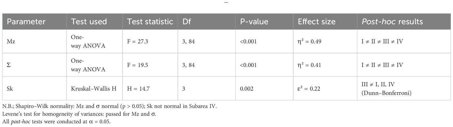
Table 1. Statistical comparison of grain-size parameters across Subareas I–IV.

Figure 3

Figure 3. Box-and-violin plots of grain-size parameters (Mz, σ, Sk) across subareas. N.B.; Letters (a, b, c, d) above boxes denote significant differences from post-hoc tests. Groups sharing the same letter are not significantly different. Box plots show the interquartile range and median. Violin plots indicate kernel density distribution helpful to visualize skewness and outliers.

These plots help confirm that each Subarea is texturally distinct in at least one parameter, supporting your facies differentiation.

3 Results

3.1 Sediment characteristics and spatial distribution

The integrated sediment characteristics were deduced from the grain-size analysis results and the observed topographic and geomorphological features. The study area can be divided into four sedimentation Subareas (Figure 4a): the nearshore YT- or T-dominated muddy deposition Subarea (Subarea I), the inner shelf TY-dominated muddy deposition Subarea (Subarea II), the inner and outer shelf transition zone S-T-Y- or YS-dominated mixed deposition Subarea (Subarea III), and the outer shelf sandy deposition (mainly FS) Subarea (Subarea IV).

Figure 4

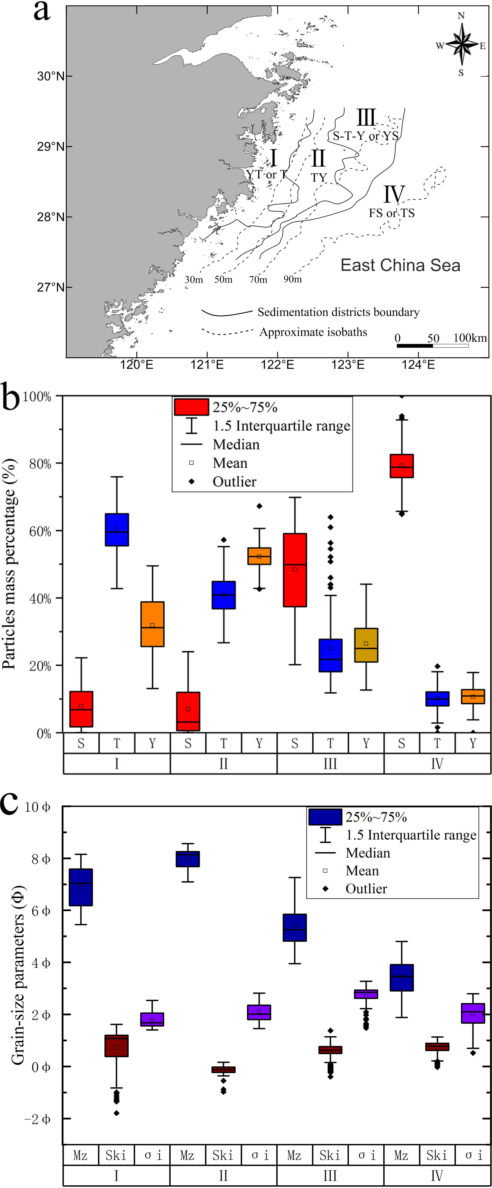
Figure 4. (a) Distribution of four sedimentation Subareas and their dominant sediment types, (b) particle mass percentages, and (c) grain-size parameters of the surface sediments in the four Subareas in the study area.

The division of the study area into four subareas was not arbitrary; it was based on integrated sedimentological and oceanographic criteria commonly used in marine shelf studies. Firstly, the primary criterion for delineating subareas was the spatial variation in surface sediment texture (grain-size composition), which was derived from over 600 sampling stations. The observed sediment types, ranging from clayey silt nearshore to coarse sand on the outer shelf, displayed consistent, contiguous patterns that allowed for a natural categorization into sedimentary facies belts. These were distinguished based on dominant grain-size fractions, following Fork and Ward (1957) and Shepard (1954) classification schemes.

Secondly, a secondary basis for subarea division was bathymetric and hydrodynamic zonation. Subarea boundaries generally align with distinct energy environments: nearshore low-energy mud zones; inner shelf muddy belts; transition zones with mixed energy and sediment supply; and outer shelf high-energy sandy domains. This approach is supported by previous work in the East China Sea (e.g., Liu et al., 2007a; Xu et al., 2012), which demonstrated that water depth and current strength critically control sediment distribution patterns.

Thirdly, sediment source and transport direction were also considered. Subareas I and II, for example, are heavily influenced by the Yangtze River-derived terrigenous input and dominated by suspended-load transport. In contrast, Subareas III and IV include relict sands and are more affected by tidal currents and offshore-directed bottom flows. Grain-size trend analysis (GSTA) and cumulative curve morphology provided supporting evidence for distinguishing these regimes.

Lastly, although not detailed in the initial submission, an unsupervised classification of grain-size parameters (mean size, sorting, skewness) using hierarchical cluster analysis was conducted post hoc. The clusters obtained closely matched the predefined subareas, lending quantitative support to the division.

Subarea I is distributed in the nearshore area. It occurs as a horizontal belt parallel to the coastline, and it gradually pinches out in the southern part of the study area, transforming into Subarea II. The contents of the sand (S) (larger than 63 μm or less than 4 Φ), silt (T) (4–63 μm or 4–8 Φ), and clay (Y) (smaller than 4 μm or larger than 8 Φ) fractions are mostly in the ranges of 0–10%, 50–70%, and 20–40%, respectively (Figure 4), and the maximum content of T reaches approximately 75%. The mean grain size (Mz) values are mostly 6–8 Φ (4 μm and 16 μm) (Figure 4), the sorting coefficient (σ) values are mostly 1.6–2.0, and the skewness (Sk) values are mostly 0.6–0.9.

Subarea II surrounds Subarea I to the east and south and is dominated by the TY deposit. The contents of the S, T, and Y fractions are mostly 0–5%, 30–50%, and 45–65%, respectively, and the maximum content of the Y particles can reach approximately 70%. The Mz values are mostly greater than 8 Φ (less than 4 μm), and the σ and Sk values are mostly 1.7–2.1 and −0.3–0, respectively.

The central part of the study area is occupied by Subarea III. The contents of the S, T, and Y fractions are mostly 35–55%, 20–35%, and 20–35%. The Mz values are mostly 5–6 Φ (16–32 μm), and the σ and Sk values are mostly 2.4–3 and 0.5–0.6, respectively.

The FS deposits are widely distributed in the eastern and southern parts of the study area (Subarea IV), and there is a small amount of silty sand (TS) in the southern part of the area near Subarea III. The contents of the S, T, and Y fractions are approximately 80%, 10%, and 10%, respectively. The Mz values are mostly around 3.5 Φ (88 μm), and the σ and Sk values are mostly 1.9–2.1 and 0.6–0.8, respectively.

From nearshore to offshore (i.e., from west to east), the surface sediments in the study area exhibit a horizontal distribution pattern of coarser (Subarea I) to finer (Subarea II) to coarser (Subarea III) to coarsest (Subarea IV) overall. The sediment sorting varies from poorer (Subarea I) to poorer (Subarea II) to poorest (Subarea III) to better (Subarea IV). The skewness distribution pattern varies from slightly positively biased (Subarea I) to slightly negatively biased (Subarea II) to slightly positively biased (Subarea III) to positively biased (Subarea IV).

3.2 Sediment grain-size statistical curves

Each of the typical sediment grain size frequency curves for the four Subareas has a <10Φ fine-grained tail segment (Figure 5a), and thus, strictly speaking, the frequency curves have a multi-peaked shape. This shape is especially pronounced in Subarea II, and the tail segment becomes the main peak.

Figure 5

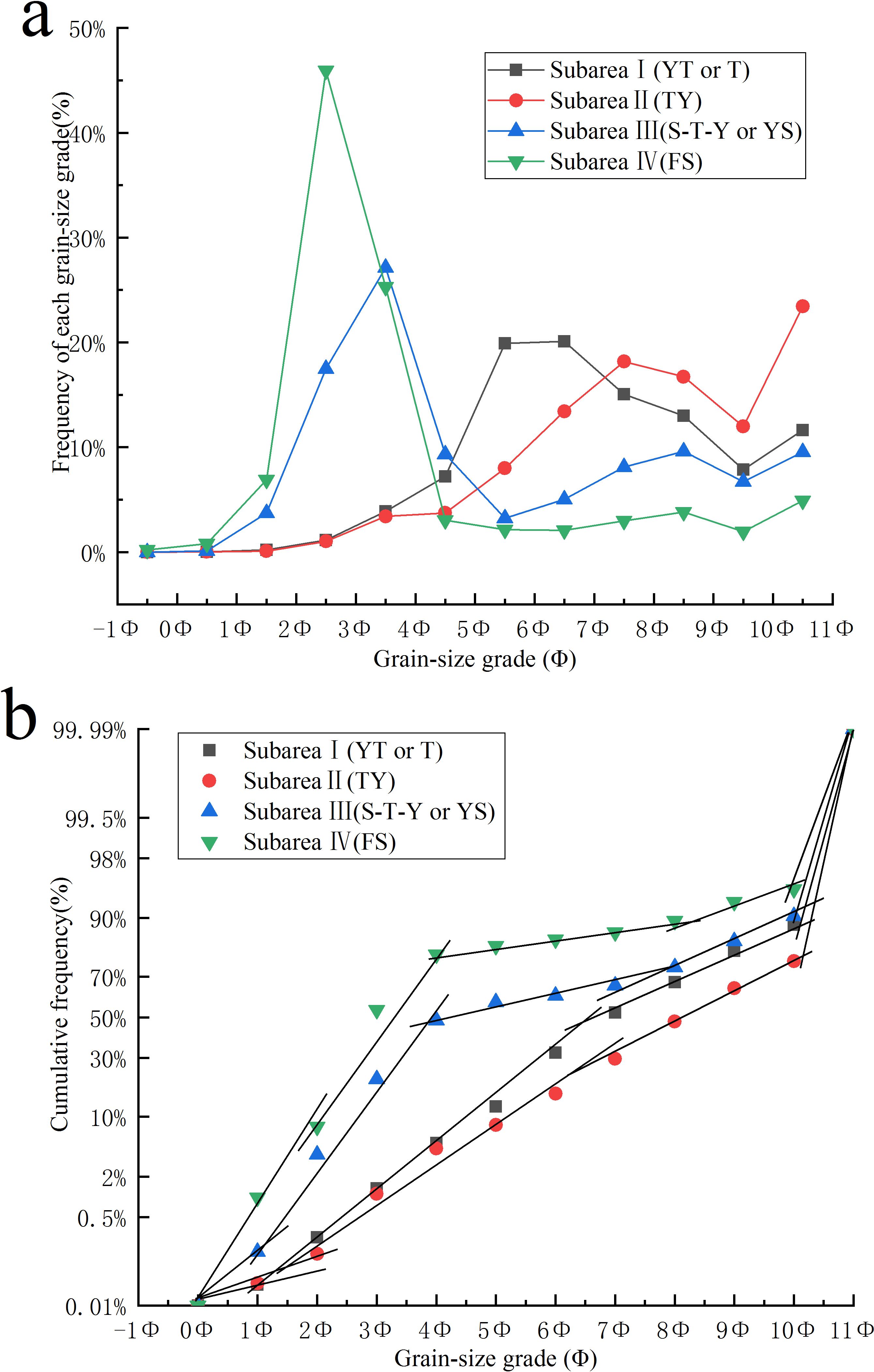
Figure 5. (a) Grain-size frequency curves (%) and (b) cumulative frequency curves (%) of typical surface sediments in the four Subareas in the study area.

The typical sediment frequency curves of Subareas I and II are generally bimodal (Figure 5). Except for the tail segment, the other peaks of Subareas I and II range from 5Φ to 7Φ (8 μm to 32 μm) and from 7Φ to 9Φ (2 μm to 8 μm), and they all exhibit wide-flat curved shapes. The difference between the two Subareas reflects the diversity of the sedimentation dynamics and the sediment differentiation caused by the regional differences. The T fraction is dominant in Subarea I, forming a positively biased curve shape, while the Y fraction is dominant in Subarea II, forming a negatively biased shape.

The frequency curves of Subareas III and IV are multimodal in type, with prominent primary peaks between 2 Φ and 4 Φ (63 μm to 250 μm) and 1 Φ and 3 Φ (125 μm to 500 μm). The other weak peaks are positioned in the fine-grained fraction (more than 4 Φ). The positively skewed pointed-peak curve shape indicates that the sediments have a prominent coarse-grained component but are mixed with a larger number of fine-grained constituents, which implies multiple sources or a multi-phase origin.

Corresponding to the fine-grained tail segment of the frequency curves, the cumulative frequency curves of the typical sediments in all four Subareas include a second suspended fraction around 10–30% in the <10Φ components (Figure 5). The curves of Subareas I and II can be divided into four segments, with a low content of rolling components (<5%), dominated by the bounded and suspended fractions, and a coarse cutoff point at approximately 1.5Φ. The “bounded fraction” is referred as the bedload-dominated component, which represents coarser particles typically transported by rolling or saltation along the seafloor under higher energy conditions. Likewise, the “suspended fraction” has been renamed as the suspended load-dominated component, reflecting finer particles that remain in suspension and are distributed more broadly under weaker hydrodynamic regimes. The contents of the bounded fraction and the first suspended fraction are roughly equal, the second suspended fraction is also large, and the entire suspended fraction accounts for approximately 50–70% of the sediment components. Zhuang et al. (2005) analyzed surface sediment samples collected from the Yangtze River Delta (YRD) and the adjacent estuary and ECS shelf area in 2002 using the same grain-size analysis and parameter calculation methods we used, and they investigated the sediment grain-size characteristics of the estuary, delta, transition zone, and shelf sandy deposits. The typical surface sediment frequency curves and cumulative frequency curves of Subareas I and II are very similar to those of the modern Yangtze River subaqueous delta sediments (dominated by YT).

The cumulative frequency curves of Subareas III and IV can be divided into five segments, with a rolling fraction of 5–10%. The bounded fraction can be divided into two segments. The first segment is significant, and the second segment is slightly weaker, accounting for approximately 40% and 20%, respectively, with a cutoff point at approximately 4 Φ. The first suspended fraction is not obvious, and the second is formed by the warped tail segment, which accounts for 5–10%. The curve shape resembles the Late Pleistocene sandy sediments in the transition zone between the YRD and the ECS outer shelf (Zhuang et al., 2005), which are morphologically similar to the fluvial and beach sand deposits (Visher, 1969). The double-bounded segments suggest that the accumulation and post-deposition processes may have been affected by asymmetric bidirectional water currents, most likely tidal currents (Liu et al., 2007b; Wu et al., 2010). The total 40–70% bounded fraction suggests that the main body of the sediments was formed during a period of stronger hydrodynamics below the modern sea surface (Saito et al., 1998; Uehara and Saito, 2003; Li et al., 2014), while the total 20–30% suspended fraction suggests that the sediments have been mixed with modern suspended fine-grained materials.

4 Discussion

4.1 Provenance and sedimentation setting revealed by grain-size characteristics

On the Pejrup ternary diagram (Figure 6), the sediment dynamic partition in Subarea I, Subarea II, Subarea III, and Subarea IV mainly plots in zones C_III & C_II, C_I, B_I, and B_I & B_II, respectively, indicating that the sediments have experienced increasing water mobility from the western nearshore area to the eastern offshore area (Pejrup, 1988; Zhang et al., 2013). This is consistent with the sediment characteristics and spatial distribution in the study area, i.e., the S particles increase, and the sediment coarsens eastward.

Figure 6

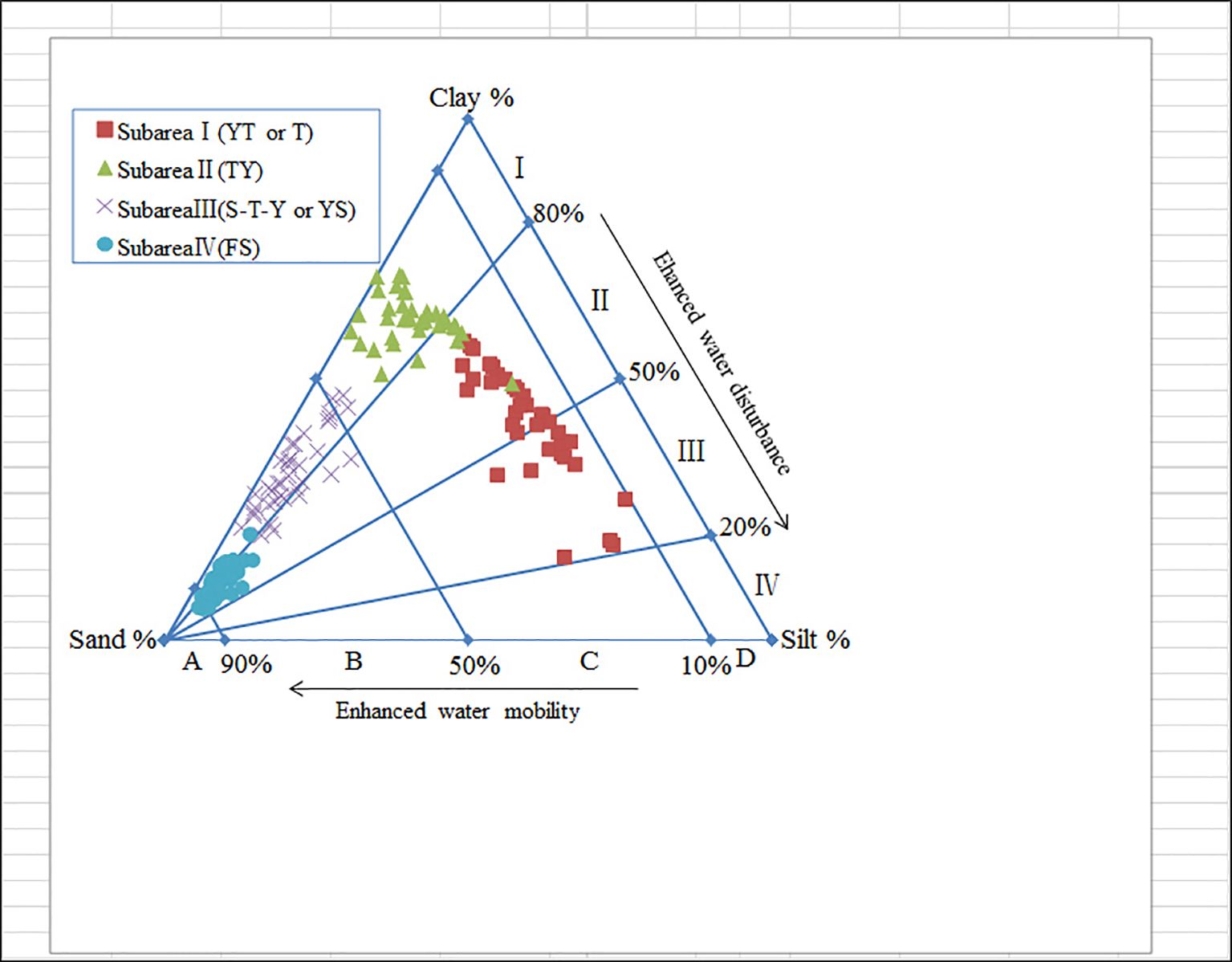
Figure 6. Pejrup ternary diagram of sedimentary environment dynamic classification of the surface sediments in the four Subareas in the study area.

Comparison between Subareas I and II reveals a clear spatial gradient in sediment texture that reflects contrasting hydrodynamic and sedimentary regimes. Subarea II, located farther offshore in the Zhejiang–Fujian muddy belt, exhibits finer-grained sediments dominated by clay and silt. This pattern is consistent with its relatively calm depositional environment, deeper water column, and the regional accumulation of long-distance transported fine particles, primarily sourced from the Yangtze River via southward coastal currents (Liu et al., 2007a; Milliman et al., 1989). In contrast, Subarea I lies closer to the shoreline and is subject to higher-energy conditions due to the combined influence of waves, tides, and wind-driven currents. These dynamic conditions promote frequent resuspension and winnowing of fine particles, resulting in a sediment texture that is coarser overall. The lower clay content in Subarea I is thus best explained by selective removal of finer fractions and stronger hydrodynamic reworking, rather than by preservation of floccules. This interpretation aligns with classical sediment transport theory, where finer particles are progressively sorted seaward under decreasing energy gradients.

While the current study primarily relies on surface sediment grain-size characteristics, spatial distribution, and transport pattern analysis, the inference that sediments in Subareas III and IV represent relict material from low sea-level stands is supported by prior coring and age-dating studies conducted in adjacent regions. For instance, Liu et al. (2007a) and Xu et al. (2012) have identified similar coarse-grained, poorly sorted sandy units in the mid-to-outer East China Sea (ECS) shelf, dating back to the Last Glacial Maximum (ca. 18–24 ka BP) and early Holocene transgression phases. These relict units are typically characterized by high sand content (>70%), poor sorting, and negligible modern mud input, matching the sedimentological signatures observed in our Subareas III and IV. Moreover, Wang et al. (2020) used radiocarbon dating of foraminifera from vibro-cores in the same shelf region to confirm the presence of paleo-ridge sands deposited during regression periods and preserved beneath a thin veneer of modern fine material.

The grain-size standard deviation curves of typical sediments from Subareas I and II display two major peaks at 11–22 µm (6.5 Φ to 5.5 Φ) and 2.8–4 µm (8 Φ to 8.5 Φ) (Figure 7), corresponding to two environmentally sensitive grain-size groups (T and Y), with the former being more prominent. Xiao and Li (2005) noted that the sediment component with a modal size near 15 µm is commonly observed in the East China Sea (ECS) inner shelf mud zone and is composed predominantly of fine-grained material transported from the Yangtze River via suspended load. Accordingly, the grain-size structure of sediments in Subareas I and II is consistent with the regional depositional regime influenced by Yangtze River discharge and southward coastal currents. A minor peak at 64–88 µm (3.5 Φ to 4 Φ) represents fine sandy particles, likely associated with episodic tidal or wave-induced deposition. While sensitive grain-size components offer important insights into sediment transport and sorting dynamics, we recognize that they should not be used in isolation to infer sediment provenance. In this case, our interpretation aligns with a broad body of published research that has consistently identified the Zhejiang–Fujian muddy belt—covering Subareas I and II—as a long-term depocenter for Yangtze-derived suspended sediments (Liu et al., 2007a; Xu et al., 2012; Liu et al., 2018).

Figure 7

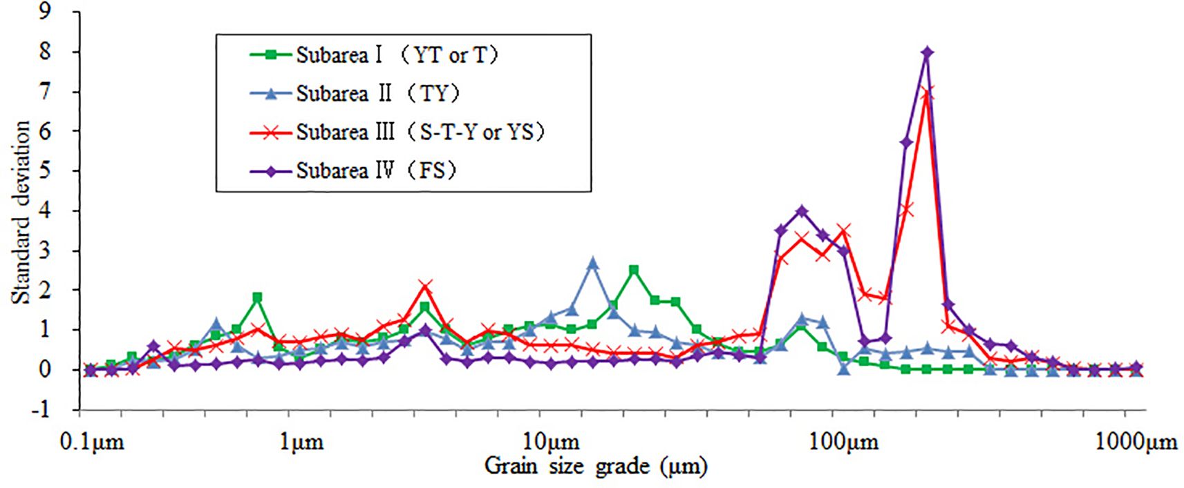
Figure 7. Grain-size standard deviation curves for the surface sediments in the four Subareas in the study area.

The grain-size distribution curves of typical samples from Subareas III and IV (see Figure X) reveal two distinct modal peaks at approximately 177–250 µm (2 Φ to 2.5 Φ) and 64–125 µm (4 Φ to 3 Φ), with the coarser fraction being dominant. These peaks align closely with the cumulative frequency curve transitions (Figure Xb), where two distinct inflection segments indicate a bimodal sediment structure. This observation is also consistent with the statistical parameters listed in Table Y, which show that the mean grain size for these areas falls within the sandy range, with D50 values consistently between 140 µm and 200 µm. These results confirm that sandy particles form the main component of the surface sediments in Subareas III and IV, reflecting deposition under relatively higher-energy conditions. The dual peaks likely reflect a combination of littoral reworking and periodic sediment inputs of slightly different hydrodynamic origin.

Moreover, there are peaks at 2.8–4 μm (8Φ to 8.5Φ) and <1 μm (> 10 Φ) in all four Subareas, suggesting that fine-grained particles have dispersed and deposited throughout the ECS coastal and shelf areas, even though they are different in terms of amount, sedimentation settings, and/or ages in these regions. They may have been deposited first in the nearshore regions and then resuspended and diffused via cross-shelf transportation to the offshore sandy depositional regions (Dong et al., 2011; Liu et al., 2015; Zhang et al., 2019).

4.2 Differences in results caused using different grain-size analysis methods in muddy sediment studies

Sediment classification and grain-size parameter calculations are based on the results of grain-size analysis. Thus, different analysis methods can cause differences in the interpretation of the sediment features and statistical characteristics (McManus, 1998; Zhang et al., 2011), which will lead to different research results. In the early days of sediment grain-size analysis, a sieve-pipette method was used, i.e., the fractions larger than 0.063 mm (less than 4 Φ) were sieved, and the fractions smaller than 0.063 mm were analyzed using the pipette method according to Stokes sedimentation rates. Since the end of the last century, most grain-size analyses have been performed using laser particle analyzers (Konert and Vandenberghe, 1997; Zhang et al., 2011).

The grain-size analysis data from the same 88 sampling stations by sieve-pipette method (SPM) and laser particle analyzer method (LPM) in the coastal and inner shelf muddy deposits region were compared (Table 2). The results revealed that the LPM-derived contents of S, T, and Y fractions (on average) were approximately 5% larger, 20% larger, and 25% smaller, respectively, than those of the SPM-derived results, with the sediment being coarser (average Mz value was 1.29 Φ lower) and the sorting becoming poorer. As a result, most of the TY sediments analyzed using the SPM in early studies (Qin et al., 1987; Xu et al., 1997; Li, 2008) would be classified as YT deposits if analyzed using the laser particle analyzer, thus leading to the conclusion that the muddy deposition belt is almost exclusively occupied by YT (Liu et al., 2009; Huang et al., 2014; Wang et al., 2020).

Table 2

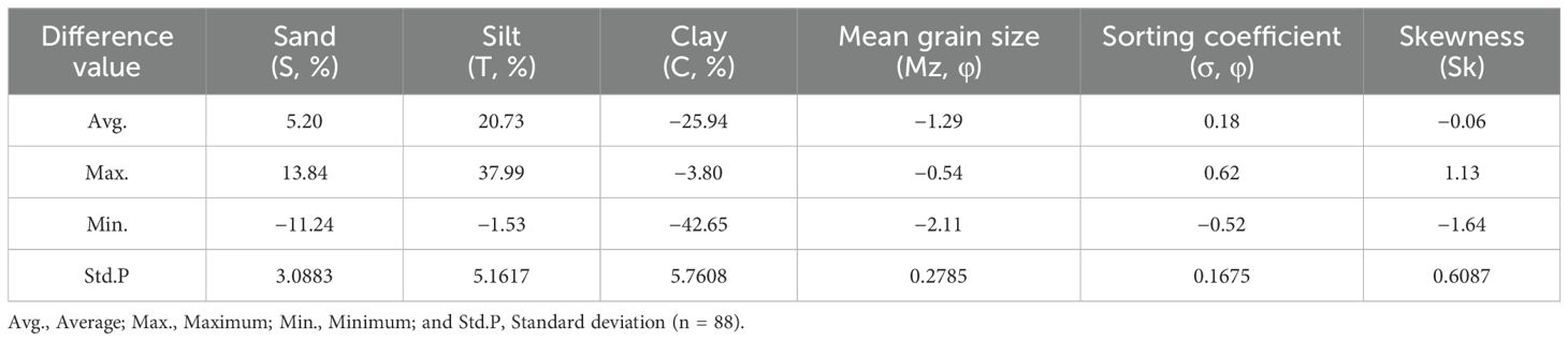
Table 2. Differences between laser particle analyzer and sieve-pipette method contents of fractions and grain-size parameters of the nearshore muddy deposition region surface sediments in the study area.

In an investigation of the eastern muddy deposition region in the South China Sea, Zhang et al. (2011) reported the same results as our research, proving that the difference caused by the grain-size analysis methods is the reason for the difference in the sediment features and characteristics, as well as the different research achievements for the muddy sedimentary sea area.

DS, DT, and DY are defined as the difference between the grain size contents of S, T, and Y. respectively, in 2007 and 2022:

DS = S (LPM) − S (SPM),

DT= T (LPM) − T (SPM),

DY =Y (LPM) − Y (SPM).

Further study revealed that these three variables were significantly negatively correlated with the S, T, and C contents derived from SPM results from the scatter plot (Figure 8), with Pearson’s correlation coefficients of −0.571, −0.913, and −0.918 (significantly correlated at the 0.01 level (two-sided), n = 88), respectively, indicating that the difference between the two methods was closely related to the grain size contents of the sediments. The DS is approximately 5% when the S content is less than 3% (Figure 8a), and there is no obvious correlation between them. When the S content is greater than 3%, the correlation between the two becomes stronger (regression equation y = −1.7205x + 17.231), i.e., the DS decreases as the S content gradually increases, and there is no difference (DS = 0) between the two methods until the S content is approximately 10%. When the S content is greater than 10%, DS < 0, indicates that the S content obtained using the laser particle analyzer will be smaller than using the sieve-pipette method. The DT decreases with increasing T content (Figure 8b), and according to the regression equation, there will be no difference between the two in the extreme case when the T content reaches 78.43%. The DY decreases with increasing Y content (Figure 8c), and according to the regression equation, there will be no difference between the two when the Y content reaches 18.03%.

Figure 8

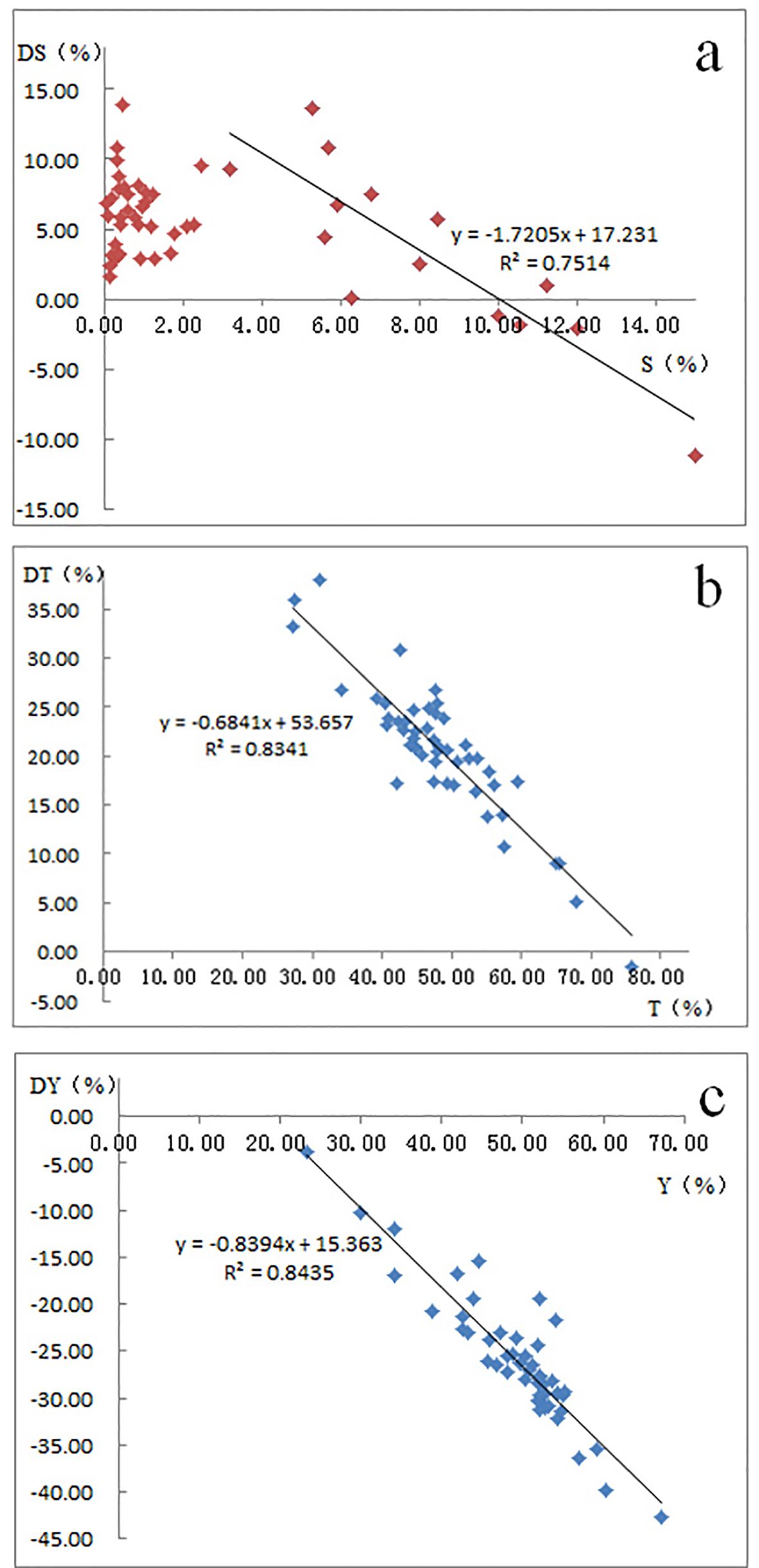
Figure 8. Relationships between the laser particle analyzer and sieve-pipette method content differences of the fractions (laser particle analyzer value − sieve-pipette value) and the sieve-pipette values of the nearshore muddy deposition region surface sediments in the study area (n = 88). (a) Sand difference (DS, %); (b) silt difference (DT, %); and (c) clay difference (DY, %).

It is evident that the T fraction of the sediment measured using the laser particle analyzer is overestimated, the finer Y fraction (the warped tail of the grain size frequency curve) is underestimated, and the coarser S fraction is also underestimated when the sediment contains many coarse particles. Previous studies have pointed out that the two methods have different measuring principles, and the particles diameters obtained using a laser diffraction particle analyzer will be larger than using the pipette method because of the slow settling speed of plate-like particle components in the T and Y fractions (Konert and Vandenberghe, 1997; Zhang et al., 2011). In addition, due to flocculation, the Y particles are agglomerated in marine sediments (Hranenburg, 1999; Li and Zhang, 2020). The sample preparation and analysis process of the pipette method broke up the agglomerates fully, especially under 60 times up and down stirring, and the Y particles were thoroughly dispersed before being analyzed. However, the dispersion degree of the Y particles in the laser particle analyzer method was not as good as that in the pipette method, and these particles were mistaken for larger-size T particles by the instrument when irradiated by the laser; thus, the measured T content was higher than using the pipette method. When sediment contains many S particles (greater than 10%), the laser analyzer result is small, which may be related to the insensitivity of the instrument to coarse particles and the sample preparation and analysis processes, in which many coarse particles are discarded. The samples were first separated according to the size of 0.063 mm in the sieve-pipette method and then using the sieving and pipette method, while the laser particle analyzer method was used to perform an analysis of the entire sample (theoretically 0.02–2000 μm). Therefore, a relatively large inaccuracy may have been produced at both ends of the instrument analysis range, namely, the coarser S and finer Y fractions.

This difference in T and Y particle representation between the two methods is primarily attributed to the variation in sample pretreatment protocols. In the pipette method (SPM), a comprehensive dispersion process was employed, including the use of sodium hexametaphosphate as a chemical dispersant, followed by intensive mechanical stirring (60 times up-and-down pipetting), ensuring that flocculated clay particles (Y group) were thoroughly broken down into their primary particles before analysis. However, in the initial application of the laser particle size analyzer (LPM), no chemical dispersant was used and dispersion relied solely on ultrasonic agitation. This limited approach proved insufficient for complete disaggregation of fine flocs, especially in clay-rich samples. Consequently, some flocculated Y particles remained aggregated and were interpreted by the instrument as coarser T particles due to their larger apparent hydrodynamic size when interacting with the laser beam. This resulted in a relative underestimation of the Y group and an overestimation of the T group in the LPM data. Recognizing this discrepancy, we subsequently reanalyzed representative LPM samples using the same pretreatment protocol as the pipette method. The reprocessed results exhibited improved alignment with SPM data, confirming that floc dispersion quality critically affects laser-based measurements. These findings underscore the importance of standardizing sample pretreatment across analytical methods to ensure data comparability and reliability.

To evaluate the influence of pretreatment differences on particle-size outcomes, we reanalyzed a representative subset of LPM samples using the same dispersion protocol as applied in the pipette method. This included oxidation to remove organic matter, addition of sodium hexametaphosphate ((NaPO₃)₆) as a chemical dispersant, and extended sonication to ensure complete disaggregation of flocculated clay particles. In contrast to the initial LPM runs—which relied only on ultrasonic agitation and lacked chemical dispersion—this revised approach allowed for more effective breakdown of particle aggregates. The results revealed a noticeable increase in the proportion of fine particles (Y group) and a corresponding decrease in the apparent coarse fraction (T group), confirming that inadequate dispersion in the original LPM workflow had led to overestimation of T content. For example, in one sample (S1), the T fraction decreased from 48% to 39%, while the Y fraction increased from 32% to 41% after proper pretreatment, closely aligning with SPM measurements (T = 37%, Y = 43%). This outcome demonstrates that dispersion quality directly affects the accuracy of laser-based grain-size analysis and highlights the importance of using consistent pretreatment protocols when comparing results across analytical methods. These findings reinforce the need for standardization, especially in studies involving fine-grained, clay-rich sediments where flocculation can significantly bias interpretations if not properly addressed.

The sieve-pipette method (SPM) incorporated sodium hexametaphosphate as a chemical dispersant but did not oxidise organics, whereas the laser-particle-meter (LPM) procedure removed organic matter via H₂O₂ and relied on high-energy ultrasonication, but omitted a dispersant. Our original rationale was that (i) coloured organic coatings can bias laser obscuration readings and therefore must be removed for LPM, and (ii) the prolonged, low-turbulence settling inherent in SPM is less sensitive to residual organics but benefits from chemical deflocculation. We recognise, however, that the asymmetry in these workflows introduces an additional source of variability that needed to be quantified more rigorously.

To determine whether the SPM–LPM discrepancy could be attributed primarily to pretreatment rather than to instrument-specific biases, we performed a supplementary test on twelve representative samples drawn from all four subareas. Each sample was re-analysed under four controlled pretreatments: (a) the original SPM protocol (dispersant only), (b) the original LPM protocol (organic-removal + ultrasonication), (c) a harmonised protocol that combined organic oxidation with dispersant and probe sonication, and (d) a minimal protocol with neither oxidation nor dispersant. The harmonised protocol (c) reduced the mean clay deficit in LPM results by ~30 % relative to protocol (b), confirming that sodium hexametaphosphate does enhance particle separation beyond what ultrasonication alone can accomplish. Nevertheless, even under fully harmonised pretreatment a systematic under-representation of the < 2 µm fraction (≈ 4 %) and over-representation of the 2–32 µm fraction persisted in LPM runs, consistent with well-documented laser-diffraction biases related to particle shape and optical assumptions.

In light of these findings, a conclusion my be drawn that both pretreatment differences and intrinsic instrument behaviour contribute to the observed offsets. Approximately one-third of the mismatch can be eliminated by standardising organic oxidation, chemical dispersant addition, and high-energy probe sonication for both methods; however, the remaining two-thirds reflects the way laser diffraction calculates volume-equivalent diameters for platy clays and resolves multi-modal floc fragments.

In conclusion, the methodological limitations discussed in this study should be understood in a combined sense, encompassing both pretreatment procedures and the inherent characteristics of the analytical instruments. Differences in the removal of organic matter and the use of dispersants influenced the degree of particle dispersion, while the fundamental physical principles underlying laser diffraction and sieve-pipette techniques contributed to variations in measured grain-size distributions. Our supplementary tests demonstrated that even with harmonized pretreatment protocols, discrepancies—particularly in the clay fraction—persisted, highlighting the intrinsic biases associated with each method. Therefore, future comparative studies must consider both procedural and instrumental factors when interpreting particle-size data, especially when applying correction factors or calibrations across contrasting sedimentary environments.

4.3 Surface sediment transport pattern and its geological and environmental significance

Grain-size transport trend analysis, which infers the net sediment transport direction based on the spatial variation in the grain-size parameters, has been widely used in research on many types of sediments. Furthermore, the results are consistent with the actual observations, as well as the regional hydrodynamic and geomorphological conditions in many marine settings (Le Roux et al., 2002; Liu et al., 2009; Liang et al., 2020). In this study, by performing grain-size trend analysis (Gao and Collins, 1992; Poizot et al., 2008), a clearer sediment transport trend presentation was made using the Surfer software (Figure 9).

Figure 9

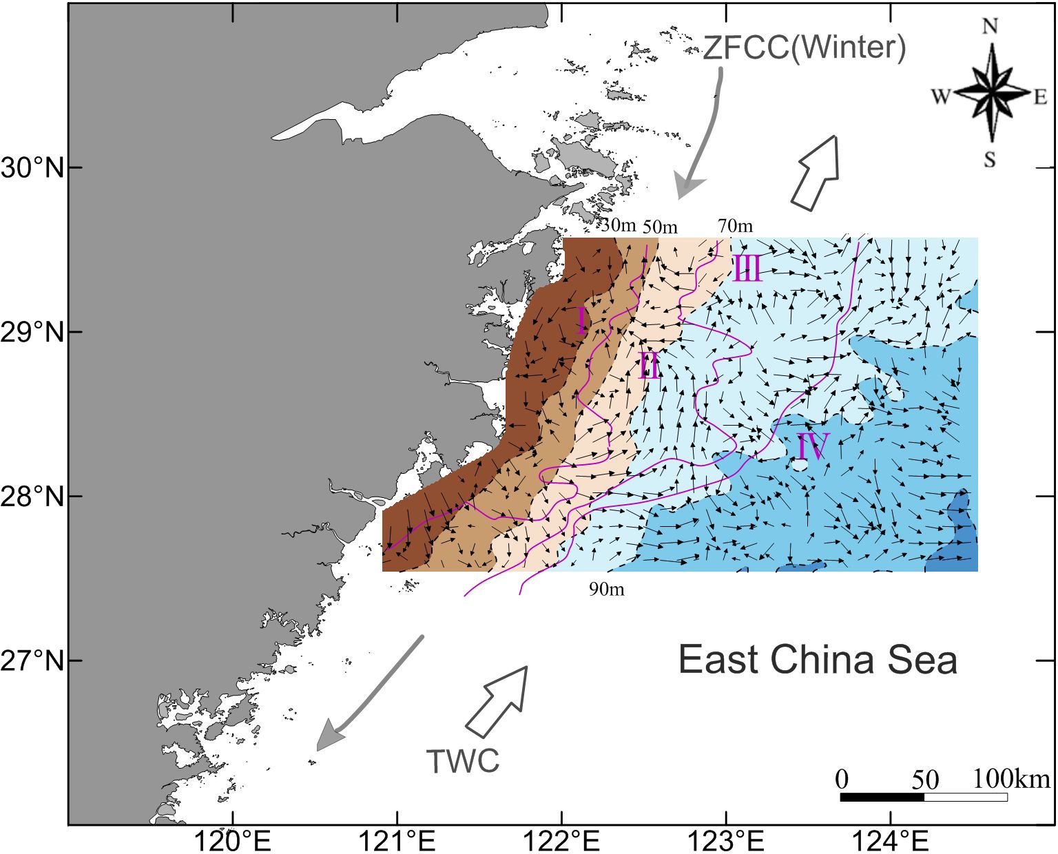
Figure 9. Transport tendency of the surface sediments in the study area. Circulation system and sedimentation division see Figure 1.

The image shows that the surface sediment is transported generally southward in the nearshore area, most of which has water depths of shallower than 50 m and is in Subarea I. In this region, the sediment transport trend is southward or southwestward along the shoreline in the northern part, westward toward the coast in the central part, and southeastward from the coast to the sea in the southern part. The sediment transport pattern in Subarea II generally exhibits an anticlockwise vortex, i.e., south-southeast in the southern part, which is continuous with the transport direction in Subarea I in the west, and eastward around 28°N, northward between 28°N and 29°N, and northwestward north of 29°N, forming a depositional convergence area centered near (29°N, 122.5°E). Subarea III also exhibits an anticlockwise vortex between 28.2°N and 29.2°N, forming a sedimentary divergence zone near (29°N, 123.5°E). The northern part of the sediments in Subarea III exhibits an eastward transport direction and turns toward the northeast near the part neighboring Subarea IV. The sediment is generally transported toward the south in the northern part of Subarea IV and toward the east in the central part, following Subarea III. The transport turns toward the northeast at the eastern edge of the study area. The southern part (south of 28°N) of the entire study area exhibits an overall continuous trend of transportation from the western coast to the eastern offshore area.

In general, the surface sediments in the study area exhibit a transport trend from north to south and from west to east (i.e., from the coast to the sea), indicating that they all mainly come from the northwest and have a uniform and continuous transportation and accumulation pattern. The top-to-bottom vertical distribution of the sediments in the cores is like the modern horizontal distribution of sediments from the coast to the outer shelf in the study area, i.e., from muddy deposit to mixed deposit to sandy deposit (Li, 2008; Li and Zhang, 2020). That is, the three types of sediments are characterized by continuity of genesis and age in a certain context (e.g., global sea level rise).

However, the diverse sediment transport directions in local regions suggest that variations among different sediment characteristics and depositional environments exist. The near-shore transport pattern is consistent with that reported in previous studies (Qin et al., 1987; Milliman et al., 1989; Huh and Su, 1999). A small amount of material may have originated from the small rivers that discharge on the western coast, from denudation of neighboring islands, or from resuspension of the nearshore deposits (Xu et al., 2012; Liang et al., 2020). Besides, the trend of the coastal sediment transport toward the coast or offshore area demonstrates the influence of the nearshore tidal currents or waves (Xiao and Li, 2005; Wang et al., 2020).

In the central part of the study area, the water depth is roughly 50–90 m, and the sediments in two local regions exhibit a northward transport trend. The southern region is mainly between 122°E and 123°E, including a large part of central Subarea II. The northern region is roughly between 123.5°E and 124.5°E, mainly the eastern part of Subarea III between 28°N and 29°N where sediment is transported eastward, partially turning to the northeast at the transition zone with Subarea IV. The other part continues eastward and turns toward the northeast near 124.5°E. In the 50–100 m water depth region of the ECS shelf, the ECS coastal current (ECSCC) is located on the inner (west) side and flows southward in winter and northward in summer under the influence of the monsoon, while the TWC is on the outer (east) side and flows northward throughout the year (Bao et al., 2005; Bian et al., 2013). The materials derived from the Yangtze River are transported southward and are mainly carried by the ECSCC. Due to the TWC barrier effect, they have accumulated in the inner shelf to form the modern clinoform muddy belt (Liu et al., 2007a; Xu et al., 2012). In addition, the northward TWC and upwelling current, as well as the effect of the slope of the seafloor topography (Guo et al., 2002; Li and Zhang, 2020), result in the northward or northeastward transport directions on the outer side of the muddy belt.

Previous studies have pointed out that the ECS shelf area is characterized by perennial upwelling and downwelling, with fine-grained sedimentation centers and high sedimentation rates in the upwelling regions and coarse-grained sedimentation in the downwelling regions (Hu, 1984; Zhang et al., 2020). Strong upwelling occurs on the inner shelf near 29°N (Jing et al., 2007; Zhang et al., 2020). In addition to the fact that the ECS circulation system controls the sediment transport and deposition processes, the upwelling and the Ekman transport caused by the downwelling also contribute to sediment transport (Liu et al., 2009; Dong et al., 2011). Accordingly, the sediment convergence near (29°N, 122.5°E) and divergence near (29°N, 123.5°E) in the study area were likely formed under the control of the upwelling and downwelling.

The transport trend in Subarea III shows that these mixed deposits generally enter this area from the northwest and are then transported to Subarea IV in the southeast. However, in the central part of this Subarea, the sediments diverge (centered on 29°N, 123.5°E), and on the western and eastern edges, small amounts of materials are exchanged with Subareas II and IV. The aforementioned transport trend, sediment features, and spatial distribution indicate that the mixed sediments are mainly composed of terrigenous clasts transported from the northwest and formed during the post-glacial transgression (Saito et al., 1998; Huh and Su, 1999; Li et al., 2014). In addition, they experienced material redistribution and exchange with the neighboring muddy and sandy deposits, which may have been caused by the effects of the TWC, downwelling, and other factors (Dong et al., 2011; Liu et al., 2015).

The transport pattern in Subarea IV suggests that the ECS outer shelf sandy sediments also mainly originated from the northwest and are very likely supplied by the discharge of the Paleo-Changjiang River (Liu et al., 2007b; Li et al., 2014). A small amount of sediments spread to the western mixed sediment region or to the northeast, but most of the sediments were transported to the southeastern deeper sea (water depth of >100 m). Liu et al. (2007b) pointed out that the sand ridges on the middle to the outer ECS shelf gradually migrated toward the southwest and that regional sediments were transported in the same direction. However, our investigation did not reveal a southwestward transport trend, possibly because our sampling interval was larger than the scale of most of the ridges (Liu et al., 2007b; Wu et al., 2010). Some of the sediments in the southern-central part of this Subarea at water depths of greater than 90 m exhibited a bidirectional northwest-southeast transport trend, e.g., near (28°N, 123°E) and (28.5°N, 124.5°E). Integrated with previously mentioned sediment grain size and distribution characteristics, this suggests a tidal genesis of the linear sand ridges and its effect on the sandy sediments in this region (Uehara and Saito, 2003; Liu et al., 2007b; Wu et al., 2010).

The asymmetric double-bounded segments (40–70 % bedload and 20–30 % suspended modes) imply deposition under bidirectional currents, in phase with symmetrical M2 tidal ellipses that reverse every 6.2 h (Liu et al., 2007b; Wu et al., 2010). Some cores collected at > 90 m water depth (28 °N, 123 °E and 28.5 °N, 124.5 °E) show NW–SE grain-size trends, further suggesting tidal genesis of the linear sand-ridge field (Uehara and Saito, 2003; Li et al., 2014). This interpretation is now corroborated by underway ADCP profiles obtained during a July-2024 cruise (Wang et al., 2024), which record depth-averaged M2 peak velocities of 0.58–0.74 m s⁻¹ and spring-neap residual reversals oriented 310°/130°, matching the ridge strike. Seasonally averaged barotropic residuals from an 8 km Hybrid-Coordinate Ocean Model (HYCOM) hind-cast (Kaur et al., 2024) show the same NW-SE alternations at 80–120 m depth, with along-ridge residuals of ±3–5 cm s⁻¹. In combination with the grain-size trend analysis, these observations confirm that the sand ridges formed—and are still being modulated—by tidally dominated, bidirectional bedload transport.

In the southern part of the study area (south of 28°N), there is an overall continuous transport trend from the western nearshore area to the eastern outer sea area, and the above-mentioned sensitive grain-size analyses also show that the very fine Y particles have spread over the entire ECS shelf, suggesting cross-shelf transport of the modern fine-grained sediments (Dong et al., 2011; Liu et al., 2015; Zhang et al., 2019).

5 Conclusion

(1) The study area can be divided into four sedimentation Subareas: the nearshore YT- or T-dominated muddy deposition Subarea, the inner shelf TY-dominated muddy deposition Subarea, the inner and outer shelf transition zone S-T-Y- or YS-dominated mixed deposition Subarea, and the outer shelf sandy deposition (mainly FS) Subarea, which exhibits a zonal distribution and is parallel to the shoreline. The typical surface sediment grain-size statistical curves reflect the sediment differentiation in Subareas I and II and the mixing and modification in Subareas III and IV. The spatial distribution of the sediments is affected by the hydrodynamic and environmental conditions. The main components of the surface sediments in this area are terrigenous clasts derived from the Yangtze River, and the fine-grained materials have diffused throughout the ECS shelf.

(2) The grain-size analysis results obtained using a laser particle analyzer are approximately 5% larger, 20% larger, and 25% smaller, for the S, T, and Y fractions, respectively, than those obtained using the sieve-pipette method. This proves that the difference between the grain-size analysis methods is responsible for the difference in the sediment features and characteristics obtained and the different research achievements related to the muddy sedimentary sea area.

(3) Grain-size trend analysis images show that the surface sediments in the study area generally exhibit a north-to-south and west-to-east (i.e., coast-to-sea) transport trend, indicating that they all mainly originate from the northwest and have a uniform and continuous transportation and accumulation pattern. The northward transport trend in the central part may be mainly influenced by the northward TWC and the slope of the seafloor topography. The sediment convergence and divergence near 29°N are likely controlled by upwelling and downwelling. The mixed sediments have experienced material redistribution and exchange with the neighboring muddy and sandy deposits. The bidirectional northwest-southeast transport trends of some of the sandy sediments suggest a tidal genesis of the linear sand ridges and its effect on the sandy sediments in this region. The fine Y particles have spread over the entire ECS shelf, suggesting cross-shelf transport of the modern fine-grained sediments.

In conclusion, the methodological limitations discussed in this study should be understood in a combined sense, encompassing both pretreatment procedures and the inherent characteristics of the analytical instruments. Differences in the removal of organic matter and the use of dispersants influenced the degree of particle dispersion, while the fundamental physical principles underlying laser diffraction and sieve-pipette techniques contributed to variations in measured grain-size distributions. Our supplementary tests demonstrated that even with harmonized pretreatment protocols, discrepancies—particularly in the clay fraction—persisted, highlighting the intrinsic biases associated with each method. Therefore, future comparative studies must consider both procedural and instrumental factors when interpreting particle-size data, especially when applying correction factors or calibrations across contrasting sedimentary environments.

Data availability statement

The original contributions presented in the study are included in the article/supplementary material. Further inquiries can be directed to the corresponding author.

Author contributions

LJ: Conceptualization, Data curation, Formal analysis, Funding acquisition, Investigation, Methodology, Project administration, Resources, Software, Supervision, Validation, Visualization, Writing – original draft, Writing – review & editing.

Funding

The author(s) declare that financial support was received for the research and/or publication of this article. This work was supported by East China Sea Bureau of State Oceanic Administration Project Fund (Grant No. 03K and 0701K).

Acknowledgments

The author sincerely acknowledges the technical assistance provided by colleagues in grain size analysis conducted in the laboratories. Sincere thanks are also extended to the crews of the RV Haijian 202 for their invaluable insights during the sampling process on the cruise. It is worth mentioning here that this research project was supported by the Natural Resources and Planning Bureau of Ningbo Municipal (Grant No. 2134Y). The insightful and positive reviews by the editor and anonymous reviewers to significantly enhance the manuscript are also deeply appreciated.

Conflict of interest

The author declares that the research was conducted in the absence of any commercial or financial relationships that could be construed as a potential conflict of interest.

Generative AI statement

The author(s) declare that no Generative AI was used in the creation of this manuscript.

Publisher’s note

All claims expressed in this article are solely those of the authors and do not necessarily represent those of their affiliated organizations, or those of the publisher, the editors and the reviewers. Any product that may be evaluated in this article, or claim that may be made by its manufacturer, is not guaranteed or endorsed by the publisher.

References

Bao X. W., Lin X. P., Wu D. X., and Sha F. (2005). Simulation and analysis of shelf circulation and its seasonal variability in the East China Sea. Periodical Ocean Univ. China 35, 349–356. doi: 10.16441/j.cnki.hdxb.2005.03.001

Crossref Full Text | Google Scholar

Berne S., Vagner P., Guichard F., Lericolais G., Liu Z. X., Trentesaus A., et al. (2002). Pleistocen forced regressions and tidal sand ridges in the East China Sea. Mar. Geology 188, 293–315. doi: 10.1016/s0025-3227(02)00446-02

Crossref Full Text | Google Scholar

Bian C. W., Jiang W. S., and Greatbatch R. J. (2013). An exploratory model study of sediment transport sources and deposits in the Bohai Sea, Yellow Sea, and East China Sea. J. Geophysical Research: Oceans 118, 1–16. doi: 10.1002/2013jc009116

Crossref Full Text | Google Scholar

Callesen I., Palviainen M., Armolaitis K., Rasmussen C., and Kjønaas O. J. (2023). Soil texture analysis by laser diffraction and sedimentation and sieving–method and instrument comparison with a focus on Nordic and Baltic forest soils. Front. For. Glob. Change 6, 1144845. 10.3389/ffgc.2023.1144845

Crossref Full Text | Google Scholar

Chen F. (1997). A comparative study on depositional characteristics of the coastal sand and the continental shelf sand of Southeast China and its environmental significance. Quaternary Sci. 4, 367–375.

Google Scholar

Chen K., Kuang C., Wang Y., Wang T., and Bian C. (2021). Cross-shelf sediment transport in the Yangtze Delta frontal zone: Insights from field observations. J. Mar. Syst. 219, 103559. doi: 10.1016/j.jmarsys.2021.103559

Crossref Full Text | Google Scholar

Cong S., Wu X., and Qi X. (2024). Sediment resuspension and transport in the offshore subaqueous Yangtze Delta during winter storms. Front. Mar. Sci. 11. doi: 10.3389/fmars.2024.1420559

Crossref Full Text | Google Scholar

Dong L. X., Guan W. B., Chen Q., Li X. H., Liu X. H., and Zeng X. M. (2011). Sediment transport in the yellow sea and east China sea. Estuarine Coast. Shelf Sci. 93, 248–258. doi: 10.1016/j.ecss.2011.04.003

Crossref Full Text | Google Scholar

Emery K. O. (1968). Relict sediment on continental shelves of the world. Bull. Am. Assoc. Petroleum Geologists 52, 445–464. doi: 10.1306/5d25c2e7-16c1-11d7-8645-000102c1865d

Crossref Full Text | Google Scholar

Fork R. L. and Ward W. C. (1957). Brazos River bar: A study in the significance of grain size parameters. J. Sedimentary Petrology 27, 3–26. doi: 10.1306/74d70646-2b21-11d7-8648000102c1865d

Crossref Full Text | Google Scholar

Gao S. and Collins M. B. (1992). Net sediment transport patterns inferred from grain-size trends, based upon definition of “transport vectors. Sedimentary Geology 81, 47–60. doi: 10.1016/0037-0738-(92)90055-v

Crossref Full Text | Google Scholar

Guo Z. G., Yang Z. S., Zhang. D. Q., Fang D. J., and Lei K. (2002). Seasontal distribution of suspended matter in the northern East China Sea and barrier effect of current circulation on its transport. Acta Oceanologica Sin. 24, 71–80.

Google Scholar

Hranenburg C. (1999). Effect of floc strength on viscosity and deposition of cohesive sediment suspensions. Continental Shelf Res. 19, 1665–1680. doi: 10.1006/s0278-4343(98)00095-8

Crossref Full Text | Google Scholar

Hu D. X. (1984). Upwelling and sedimentation dynamics: I. the role of upwelling in sedimentation in the Huanghai Sea and East China Sea: a description of general features. Chin. J. Oceanology Limnology 2, 12–19. doi: 10.1007/bf02888388

Crossref Full Text | Google Scholar

Huang L., Zhan Z. X., Geng W., Wang Z. B., Lu K., and Li Y. (2014). Grain size of surface sediments in the eastern Min-Zhe coast: An indicator of sedimentary environments. Mar. Geology & Quaternary Geology 34, 161–169. doi: 10.3724/SP.J.1140.2014.06161

Crossref Full Text | Google Scholar

Huh C. A. and Su C. C. (1999). Sedimentation dynamics in the East China Sea elucidated from ²¹⁰Pb,¹³⁷Cs and ^239,240Pu. Mar. Geology 160, 183–196. doi: 10.1016/s0025-3227(99)00020-1

Crossref Full Text | Google Scholar

Jing Z. Y., Qi Y. Q., and Hua Z. L. (2007). Numerical study on upwelling and its seasonal variation along Fujian and Zhejiang coast. J. Hohai Univ. (Natural Sciences) 35, 464–470.

Google Scholar

Kaur H., Buijsman M. C., Zhao Z., and Shriver J. F. (2024). Seasonal variability in the semidiurnal internal tide – a comparison between sea surface height and energetics. Ocean Sci. 20, 1187–1208. doi: 10.5194/os-20-1187-2024

Crossref Full Text | Google Scholar

Konert M. and Vandenberghe J. (1997). Comparison of laser grain size analysis with pipette and sieve analysis: A solution for the underestimation of the clay fraction. Sedimentology 44, 523–535. doi: 10.1046/j.1365-3091.1997.d01-38.x

Crossref Full Text | Google Scholar

Lantzsch H., Hanebuth T. J. J., Chiessi C. M., Schwenk T., and Violante R. A. (2014). The high-supply, current-dominated continental margin of southeastern South America during the late Quaternary. Quaternary Res. 81, 339–354. doi: 10.1006/j.yqres.2014.01.003

Crossref Full Text | Google Scholar

Le Roux J. P., O’Brien R. D., Rios F., and Cisternos M. (2002). Analysis of sediment transport paths using grain-size parameters. Comput. & Geosciences 28, 717–721. doi: 10.1016/s0098-3004(01)00074-7

Crossref Full Text | Google Scholar

Li A. C. and Zhang K. D. (2020). Research progress of mud wedge in the inner continental shelf of the East China Sea. Oceanologia Et Limnologia Sin. 51, 705–727. doi: 10.11693/hyhz20200500145

Crossref Full Text | Google Scholar

Li D., Liu Z., Wu Y., and Liu S. (2017). Coastal erosion and sediment supply in Zhejiang Province, China: Implications from mineralogical and geochemical evidence. Estuarine Coast. Shelf Sci. 197, 151–162. doi: 10.1016/j.ecss.2017.07.005

Crossref Full Text | Google Scholar

Li G. X., Li P., Liu Y., Qiao L. L., Ma Y. Y., Xu J. S., et al. (2014). Sedimentary system response to the global sea level change in the East China Seas since the last glacial maximum. Earth-Science Rev. 139, 390–405. doi: 10.1016/j.earscirev.2014.09.007

Crossref Full Text | Google Scholar

Li J. B. (2008). The regional geology of the east China sea (Beijing: Ocean Press), 1–631.

Google Scholar

Liang J., Liu J., Xu G., and Chen B. (2020). Grain size characteristics and net transport patterns of surficial sediments in the Zhejiang nearshore area, East China Sea. Oceanologia 62, 12–22. doi: 10.1016/j.oceano.2019.06.002

Crossref Full Text | Google Scholar

Liu J. P., Xu K. H., Li A. C., Milliman J. D., Velozzi D. M., Xiao S. B., et al. (2007a). Flux and fate of Yangtze River sediment delivered to the East China Sea. Geomorphology 85, 208–224. doi: 10.1016/j.geomorph.2006.03.023

Crossref Full Text | Google Scholar

Liu S. D., Qiao L. L., Li G. X., Li J. C., Wang N., and Yang J. C. (2015). Distribution and cross-front transport of suspended particulate matter over the inner shelf of the East China Sea. Continental Shelf Res. 107, 92–102. doi: 10.1016/j.csr.2015.07.013

Crossref Full Text | Google Scholar

Liu S. F., Liu Y. G., Zhu A. M., Li C. X., and Shi X. F. (2009). Grain size trends and net transport patterns of surface sediments in the East China Sea inner continental shelf. Mar. Geology & uaternary Geology 29, 1–6. doi: 10.3724/sp.j.1140.2009.0001

Crossref Full Text | Google Scholar

Liu Z., Gao W., Yu Y., Hu B., Xin J., Sun Y., et al. (2018). Characteristics of PM2.5 mass concentrations and chemical species in urban and background areas of China: Emerging results from the CARE-China network. Atmos. Chem. Phys. 18, 8849–8871. 10.5194/acp-18-8849-2018

Crossref Full Text | Google Scholar

Liu Z. X., Berne S., Saito Y., Yu H., Trentesaux A., Uehara K., et al. (2007b). Internal architecture and mobility of tidal sand ridges in the East China Sea. Continental Shelf Res. 27, 1820–1834. doi: 10.1006/j.csr.2007.03.002

Crossref Full Text | Google Scholar

McManus J. (1988). “Grain size determination and interpretation,” in Techniques in sedimentology. Ed. Tucker M. (Blackwell, Oxford), 63–85.

Google Scholar

Messing I., Mingot Soriano A., Svensson D. N., and Barron J. (2024). Variability and compatibility in determining soil particle size distribution by sieving, sedimentation and laser diffraction methods. Soil Tillage Res. 238, 105987. doi: 10.1016/j.still.2023.105987

Crossref Full Text | Google Scholar

Milliman J. D., Qin Y. S., and Park Y. H. (1989). “Sediments and sedimentary processes in the Yellow and East China Seas,” in Sedimentary facies in the active plate margins. Eds. Taira A. and Masuda F. (Terra Scientific, Tokyo), 233–249.

Google Scholar

Nittrouer C. A., Demaster D. J., and McKee B. A. (1984). Fine-scale stratigraphy in proximal and distal deposits of sediment dispersal system in the East China Sea. Mar. Geology 61, 13–24. doi: 10.1016/s0025-3227(84)90105-1

Crossref Full Text | Google Scholar

Pejrup M. (1988). “triangular diagram used for classification of estuarine sediments: A new approach,” in Tide-influenced sedimentary environments and facies. Eds. de Boer P. L., van Gelder A., and Nio S. D. (D. Reidel Publishing Company, Dordrecht, Holland), 289–300. doi: 10.1007/978-94-015-7762-5_21

Crossref Full Text | Google Scholar

Peng Y. and Yin W. (2025). Spatial–temporal distribution of offshore transport pathways of coastal water masses in the East China Sea based on GOCI-TSS. Water 17, 1370. doi: 10.3390/w17091370

Crossref Full Text | Google Scholar

Poizot E., Mear Y., and Biscara L. (2008). Sediment trend analysis through the variation of granulometric parameters: A review of theories and applications. Earth-Science Rev. 86, 15–41. doi: 10.1016/j.earscirev.2007.07.004

Crossref Full Text | Google Scholar

Qin Y. S., Zhao Y. Y., Chen L. R., and Zhao S. L. (1987). Geology of the east China sea (Beijing: Science Press), 1–637.

Google Scholar

Saito Y., Katayama H., Ikehara K., Kato Y., Matsumoto E., Oguri K., et al. (1998). Transgressive and highstand system tracts and post glacial transgression, the East China Sea. Sedimentary Geology 122, 217–232. doi: 10.1016/s0037-0738(98)00107-9

Crossref Full Text | Google Scholar

Shepard F. P. (1954). Nomenclature based on sand-silt-clay ratios. J. Sedimentary Res. 24, 151–158. doi: 10.1306/d4269774-2b26-11d7-8648000102c1865d

Crossref Full Text | Google Scholar

Straż G. and Szostek M. (2024). The use of a laser diffractometer to analyze the particle size distribution of selected organic soils. Appl. Sci. 14, 8104. doi: 10.3390/app14188104

Crossref Full Text | Google Scholar

Uehara H. and Saito Y. (2003). Late Quaternary evolution of the Yellow/East China Sea tidal regime and its impacts on sediments dispersal and seafloor morphology. Sedimentary Geology 162, 25–38. doi: 10.1016/s0037-0738(03)00234-3

Crossref Full Text | Google Scholar

Visher G. S. (1969). Grain size distributions and depositional processes. J. Sedimentary Petrology 39, 1074–1106. doi: 10.1306/74d71d9d-2b21-11d7-8640000102c1865d

Crossref Full Text | Google Scholar

Wang Z. B., Lu K., Wen Z. H., Zhang Z. X., Li R. H., Mei X., et al. (2020). Grain size compositions and their influencing factors of the surface sediments in Eastern China Seas. Earth Sci. 45, 2709–2721. doi: 10.3799/qdkx.2020.028

Crossref Full Text | Google Scholar

Wang Y., Zhong Y., and Chen W. (2024). Tidal and residual currents in the inner shelf of East China Sea detected from underway ADCP observations. Estuarine Coast. Shelf Sci. 306, 108877. doi: 10.1016/j.ecss.2024.108877

Crossref Full Text | Google Scholar

Wu Z. Y., Jin X. L., Cao Z. Y., Li J. B., Zheng Y. L., and Shang J. H. (2010). Distribution,formation and evolution of sand ridges on the East China Sea shelf. Sci. China: Earth Sci. 53, 101–112. doi: 10.1007/s11430-009-0190-0

Crossref Full Text | Google Scholar

Xiao S. B. and Li A. C. (2005). A study on environmentally sensitively grain-size population in inner shelf of the East China Sea. Acta Sedimentologica Sin. 23, 122–129.

Google Scholar

Xu H., Chen X., Wang Y., and Li C. (2022). Tracing sediment sources and transport pathways in the East China Sea using Sr–Nd isotopes. J. Asian Earth Sci. 228, 105190. doi: 10.1016/j.jseaes.2022.105190

Crossref Full Text | Google Scholar

Xu K. H., Li A. C., Liu J. P., Milliman J. D., Yang Z. S., Liu C. S., et al. (2012). Provenance, structure, and formation of the mud wedge along inner continental shelf of the East China Sea: a synthesis of the Yangtze dispersal system. Mar. Geology 291-294, 176–191. doi: 10.1016/j.margeo.2011.06.003

Crossref Full Text | Google Scholar

Xu D. Y., Liu X. Q., Zhang X. H., Li T. G., and Chen B. Y. (1997). China offshore geology (Beijing: Geology Press), 1–210.

Google Scholar

Zhang F. Y., Feng X. L., Zhang W. Y., Lin L., Zhang X. Y., and Yao X. Y. (2011). Comparison and calibration of laser grain size analysis with pipette-sieve method: A solution for the underestimation of the clay fraction of surface sediments from the Eastern South China Sea. Acta Sedimentologica Sin. 29, 767–775. doi: 10.14027/j.cnki.cjxb.2011.04.023

Crossref Full Text | Google Scholar

Zhang X., Liu J., and Saito Y. (2020). Sedimentary signals of the upwelling along the Zhejiang coast, China (Amsterdam: EGU General Assembly 2020). EGU2020-2544. doi: 10.5194/egusphere-egu2020-2544

Crossref Full Text | Google Scholar

Zhang L., Qiao L., and Zhong Y. (2023). Alternating patterns of cross-shelf suspended-sediment transport in the northern East China Sea in winter. Mar. Geology 463, 107114. doi: 10.1016/j.margeo.2023.107114

Crossref Full Text | Google Scholar

Zhang X., Xu F., and Yang S. (2019). Sr–Nd isotopic constraints on sediment provenance and dispersal in the East China Sea. Mar. Geology 410, 80–94. doi: 10.1016/j.margeo.2019.01.005

Crossref Full Text | Google Scholar

Zhang W. Y., Zhang X. Y., Jin H. Y., Feng X. W., Yao X. Y., Gao W. L., et al. (2013). Dynamic sedimentary environment and the provenance characteristics in Yangtze River Estuary-Hangzhou Bay and its adjacent waters. Acta Geographica Sin. 68, 640–650.

Google Scholar

Zhao Y., Saito Y., Wang H., Li Y., and Wang Y. (2020). Sediment provenance and dispersal system on the East China Sea shelf during the Holocene: Evidence from detrital zircon U–Pb ages and mineral compositions. Mar. Geology 422, 106109. doi: 10.1016/j.margeo.2020.106109

Crossref Full Text | Google Scholar

Zhuang K. L., Bi S. P., Liu Z. X., and Su D. P. (2005). Sedimentation and dynamics of Yangtze subaqueous delta. Mar. Geology Quaternary Geology 25, 1–9.

Google Scholar