Multifrequency backscatter classification of seabed sediments using MBES: an integrated approach with ground-truth validation

Accurate seabed sediment classification is essential for mapping marine geological features, assessing benthic habitat, and planning coastal infrastructure. This study investigated the utility of multifrequency multibeam echosounder (MBES) backscatter data for improving seabed sediment classification compared to traditional single-frequency approaches. MBES data were acquired at three frequencies (170, 300, and 450 kHz), and post-processed to produce frequency-specific backscatter mosaics and a composite red–green–blue image. Classification was performed using unsupervised clustering methods, including K-means and isodata clustering, with input vectors composed of normalized backscatter intensities from the three frequencies. The integrated multifrequency approach successfully identified three distinct sediment classes, which were validated using grab samples analyzed for grain size, water content, total organic carbon, and slope. These classes exhibited strong correspondence with underlying geomorphological features and local hydrodynamic regimes, confirming the influence of topography and tidal currents on sediment distribution. Lower-frequency data (170 kHz) were more sensitive to subsurface variability, while higher-frequency data (450 kHz) captured surface texture differences more effectively. The combined use of all three frequencies improved classification performance, particularly in transitional sediment zones where single-frequency methods proved ambiguous. The methodology proved robust across varying water depths, sediment types, and complex seabed terrains, aligning with recent advances in MBES-based sediment mapping and supporting its general applicability for other dynamic coastal systems. These results demonstrate that the use of multifrequency MBES backscatter data enhances the resolution and reliability of sediment classification results, providing a robust framework for high-resolution seabed mapping in dynamic coastal environments.

1 Introduction

Seabed sediments have physical and geochemical properties that influence the acoustic response of the seafloor and reflect critical processes related to sediment transport, deposition, and benthic habitat formation. Accurate classification of sediment types, typically categorized as gravel, sand, silt, and clay, is essential for marine geological mapping, environmental monitoring, and geotechnical planning. Seabed sediment information is needed for various marine applications, including resource exploration, habitat assessment, naval operations, and coastal infrastructure development (Goff et al., 2000; Wildish et al., 2004; Simons and Snellen, 2009; Malik, 2019).

For example, Gaida et al. (2018) applied multifrequency MBES and Bayesian classification in the Bedford Basin, Canada, revealing the utility of low frequencies for identifying deeper, coarser layers and high frequencies for resolving fine surface boundaries. Runya et al. (2021) demonstrated that combining low (30 kHz) and high (95–300 kHz) frequencies in the North Sea enhanced sediment and habitat discrimination over single-frequency approaches. Most recently, Misiuk et al. (2024) showed that multifrequency backscatter is a key variable for predicting sediment variability in the high-energy Bay of Fundy, and that such mapping directly benefits channel management, engineering, and ecosystem conservation. Other recent works (Menandro et al., 2022; Bai et al., 2023) confirm that multifrequency acoustic techniques can reliably distinguish between fine- and coarse-grained environments and provide essential information for marine spatial planning and infrastructure design.

Multibeam echosounder (MBES) systems provide two critical types of acoustic data: high-resolution bathymetric measurements and acoustic backscatter intensity. While bathymetric data describe seafloor morphology, backscatter intensity captures information related to sediment composition, grain size, compaction, and surface roughness (Gavrilov et al., 2005; Lurton et al., 2015). Due to their stability and simplicity, traditional single-frequency MBES systems are widely used for long-term monitoring and regional comparisons. However, their limited spectral resolution can hinder the accurate classification of heterogeneous or transitional seabed environments (Malik, 2019).

To overcome these limitations, recent studies have explored the use of multifrequency or multispectral backscatter data. By simultaneously acquiring data at multiple acoustic frequencies, MBES systems capture both deep-penetrating, low-frequency returns and high-resolution surface responses. Lower frequencies (e.g., 170 kHz) are more sensitive to subsurface layers and volumetric scattering, whereas higher frequencies (e.g., 450 kHz) emphasize surface texture, sediment microstructure, and roughness (Gaida et al., 2018; Khomsin et al., 2021; Schulze et al., 2022). Integrating information across frequencies enhances sediment classification capability and facilitates the detection of subtle seafloor variation that could be missed by single-frequency methods.

Despite these advantages, the application of multifrequency MBES involves increased complexity in terms of system calibration, frequency synchronization, and signal correction. Moreover, differences in scattering mechanisms between frequencies necessitate careful interpretation to avoid classification errors (Gaida et al., 2018; Fezzani et al., 2021). Therefore, the systematic evaluation of frequency-specific responses is required to ensure robust reproducible sediment classification.

This study assessed the effectiveness of multifrequency MBES backscatter data for characterizing seabed sediment types within a dynamic tidal flat environment. Using three acoustic frequencies (170, 300, and 450 kHz), we compared classification results based on individual frequency bands with those obtained using an integrated multifrequency approach. Unsupervised clustering algorithms were applied to normalized backscatter data to delineate sediment classes, which were validated using ground-truth samples and sedimentological analyses.

By quantifying the advantages of spectral integration and highlighting its role in capturing both surface and subsurface sediment variability, this study offers new insights into the application of multifrequency MBES to seabed mapping. Our findings support the development of improved sediment classification frameworks to enhance marine spatial planning, environmental impact assessment, and benthic habitat monitoring.

2 Materials and methods

2.1 Study area

The study area was Asan Bay, a semi-enclosed bay located on the western coast of the Korean Peninsula, between Chungcheongnam and Gyeonggi Provinces (Figure 1A). The bay is approximately 40 km long and 2.2 km wide, and is characterized by strong tidal forces, complex current patterns, and a diverse marine topography, including extensive tidal flats. These characteristics make the bay important for marine environmental research and coastal management (Korea Hydrographic and Oceanographic Agency (KHOA), 2009; Chang and Nam, 2011).

Figure 1

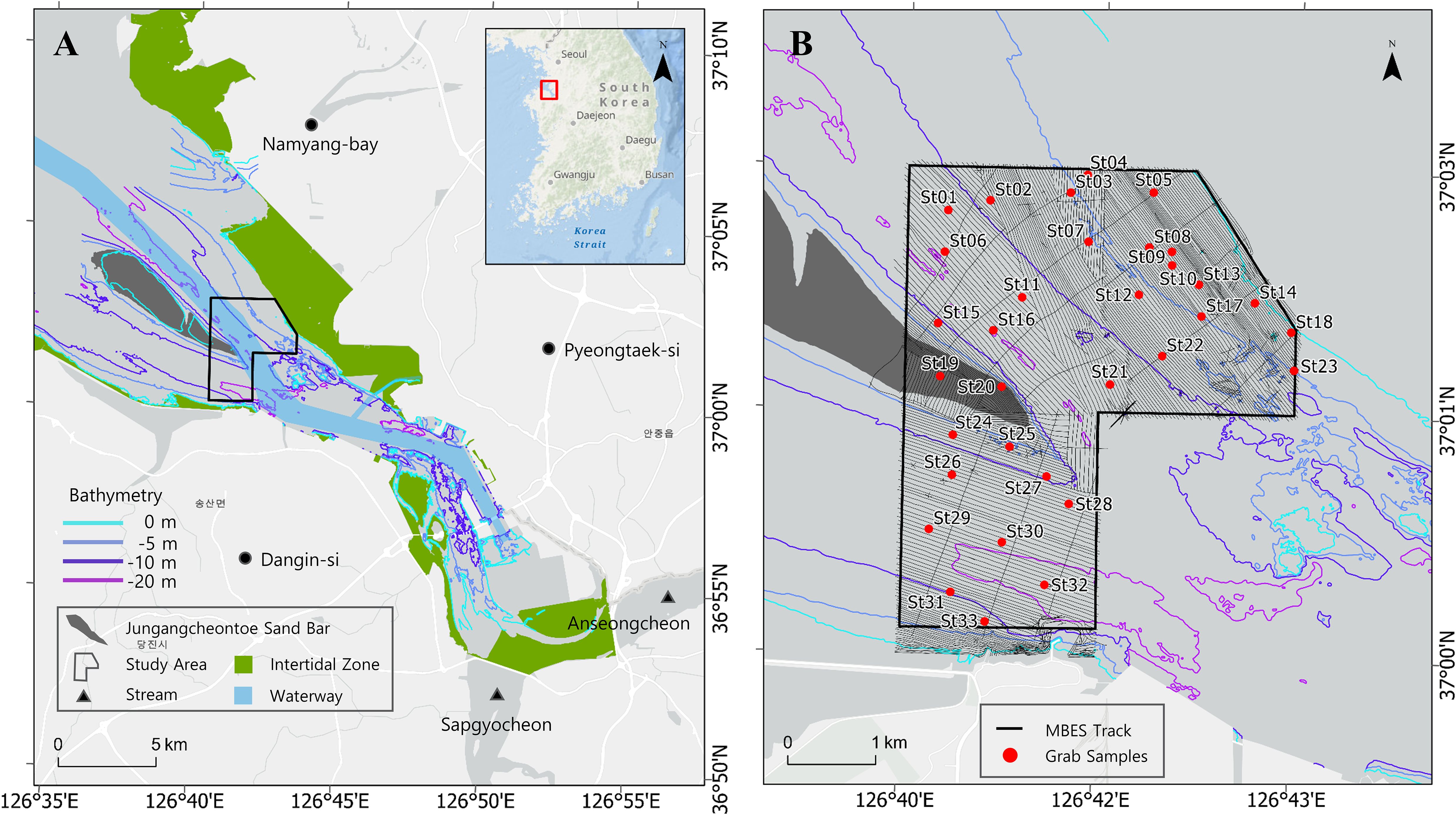
Figure 1. (A) Location of the study area in Asan Bay; the inset map shows its position on the Korean Peninsula. Bathymetric contours at 0, –5, –10, and –20 m are overlaid for reference. (B) Detailed bathymetric map of the survey area with 5-m color contour intervals. Multibeam echosounder (MBES) survey lines and grab sampling stations (red circles) are indicated.

Continuous seabed morphological changes in Asan Bay occur primarily due to sediment influx from the Geum River estuary and Yellow Sea, combined with strong tidal influences. These processes influence the marine ecosystem dynamics of the bay. Seasonally, it is influenced by the northwestern monsoon in winter and the temperate monsoon in summer, with over 55% of the annual precipitation concentrated during the flood season between June and August (Jeong et al., 2016).

Asan Bay has a mixed semidiurnal tidal regime characterized by a large tidal amplitude, with average tidal ranges exceeding 5 m (Jeong et al., 2016). These pronounced tidal fluctuations facilitate strong tidal currents throughout the bay. The central sand ridge (Joongangcheon-tui), located centrally in the outer tidal channel of Asan Bay, is predominantly sandy, partially exposed during low tide, and entirely submerged at high tide. Its foundation is confined by bedrock and adjacent islands.

Freshwater input into the bay is minimal, as major rivers in the vicinity are obstructed by dams: the Namyang seawall to the north, Asan seawall to the west, and Sapgyo seawall to the southeast. Consequently, sediment supply from riverine sources is limited. Thus, the area consists of a sandy depositional body within a macro-tidal outer bay tidal channel environment, characterized by low wave heights generally less than 1 m (Korea Hydrographic and Oceanographic Agency (KHOA), 2008, 2009; Chang and Nam, 2011). Freshwater discharge primarily occurs during summer via drainage sluices integrated into the seawalls, with recorded annual discharge volumes of 891, 940, 151, and 241 × 10⁶ m³/year. The discharges from the Sapgyo and Asan seawalls are substantial compared to other sources (Bang et al., 2013).

Water depths in the study area range between 5 and 22 m, with 16–20-m-deep tidal channels flanking the central sand ridge. Areas adjacent to the shoreline outside these tidal channels are shallower, ranging between 4 and 6 m, and often feature flat terrain, some of which is exposed at low tide (Figure 1).

2.2 MBES system description and frequency specifications

Bathymetric and backscatter data were acquired from the study area in August 2021 using an MBES system. The primary goal of the survey was to characterize the seafloor topography and sediment properties. High-resolution bathymetric and backscatter data were collected to support detailed analysis of seabed topography and sediment properties.

The survey was conducted using Marine 101, a 19-m-long survey vessel equipped with an R2Sonic 2024 MBES system, hull-mounted at the center of the vessel to ensure optimal stability and precision during data collection (R2Sonic, 2017). Integrated with the MBES transducer were a Valeport sound velocity probe and POS MV WaveMaster inertial navigation system (INS). The sound velocity probe enabled real-time corrections for acoustic velocity changes in the water column, while the INS system compensated for vessel movements such as pitch, roll, and yaw, enhancing data precision and accuracy.

The vessel also had a centrally mounted Trimble Global Positioning System antenna, providing high-precision positioning data to minimize positional uncertainty during data acquisition. This setup was essential to ensure accurate post-processing and interpretation of bathymetric and sediment data. All onboard measurement systems were integrated and operated using HYSWEEP software on a dedicated data acquisition computer installed in the wheelhouse. This configuration allowed real-time monitoring and recording of bathymetric and acoustic backscatter data, facilitating immediate quality assurance and control during the survey.

To ensure the accuracy of the acoustic measurements, a standard patch test was conducted prior to the main survey to calibrate the roll, pitch, yaw, and latency offsets of the MBES system. The MBES system used in this study was operated at frequencies of 170, 300, and 450 kHz. Frequency-dependent absorption and geometric spreading coefficients were calculated for each frequency based on the in situ water temperature (23.4°C) and salinity (32 PSU) (Table 1). The optimal system settings, including a power setting of 201 dB, a gain of 11 dB, and a pulse length of 95 μs, were determined based on the results of the patch test and simultaneous sonar-parameter trials, minimizing variation in backscatter intensity and improving the consistency of the acoustic mosaics.

Table 1

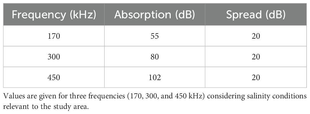
Table 1. Frequency-dependent absorption and geometric spreading coefficients for acoustic signals in seawater.

During the MBES survey, the sound velocity profile was measured along with conductivity, temperature, and depth (CTD). These additional measurements were crucial for identifying spatial variation in the underwater sound velocity, to address acoustic refraction issues that might distort depth measurements. The acquired sound velocity profile data were incorporated during MBES data processing, significantly reducing bathymetric distortion and enhancing the reliability of the resulting depth and backscatter datasets (Lurton et al., 2015).

Backscatter intensity data collected during surveys are sensitive to variables such as the source level, gain, and seawater physical properties (e.g., temperature, salinity, and density). Variation in these parameters during data acquisition, influenced by the time of measurement, water temperature, and survey location, can result in inconsistencies in backscatter mosaic images (Schimel et al., 2018). To mitigate this potential variation and ensure consistent data quality, preliminary trial surveys were conducted to establish the optimal MBES operational parameters, which were then applied consistently during the main survey.

To characterize sediment properties in the survey area, sediment samples were collected at 33 stations using a grab sampler deployed from the survey vessel. The locations of these sampling stations are shown in Figure 1B. Photographic documentation of each sediment sample enabled detailed records of sediment physical characteristics and distribution, supporting systematic analyses of seabed sedimentary environments.

2.3 Data processing and post-processing

Raw bathymetric data were corrected using real-time KHOA tidal observations. Accurate tidal data are crucial for enhancing the precision of bathymetric measurements during data collection and processing.

The bathymetric data were post-processed using Caris HIPS and SIPS v10.4. This process involved several steps. First, erroneous data were identified and removed to enhance data quality; then, sound velocity corrections were applied to reduce uncertainties associated with variations in the speed of sound within the water column; finally, tidal corrections were made to account for temporal changes in sea surface elevation, resulting in accurate final depth measurements.

Acoustic backscatter energy rapidly decreases with distance from the source due to spherical spreading, absorption, and scattering losses (Augustin et al., 1996). To compensate for this loss, time-varying gain, absorption correction, and transmission loss adjustments were applied. Since the recorded backscatter levels include artificial compensation, it is essential to remove these corrections to compute the actual bottom strength (BS) values. QPS FMGT software performed radiometric corrections including georeferencing, TVG removal, source level and beam pattern adjustments, transmission loss compensation, and ensonified area correction, thereby standardizing the backscatter data.

To further account for the influence of environmental factors such as tides, currents, and water column variability, all required parameters, including sound speed profiles, temperature, and salinity, were measured in situ and incorporated into the data processing workflow. Frequency-dependent sound attenuation and absorption coefficients were calculated using in situ CTD data, and these coefficients were integrated into the post-processing workflow to enhance the reliability of frequency-specific backscatter data.

QPS FMGT allows signal separation by frequency from multibeam acoustic datagrams and generates individual backscatter mosaics for each frequency band (170, 300, and 450 kHz). This software was used to analyze backscatter characteristics across different frequencies. The only frequency-specific radiometric correction applied by FMGT was the frequency separation itself, with additional corrections, such as beam-width adjustments, automatically implemented by the software.

The data were normalized using a moving average method based on datasets comprising 300 pings to generate angle-response curves. The reference value for normalization was derived by averaging backscatter intensity values within an incidence angle range of 30°–60° (centered at 45°), subsequently used for data normalization.

The final bathymetric data were exported as ASCII files containing x, y, and z coordinates at 0.5-m intervals. Similarly, the backscatter intensity data were exported as ASCII files (x, y, and backscatter intensity) at the same spatial resolution. These datasets were then analyzed using geographic information system (GIS) software and validated by comparison with ground-truth data.

Sediment grain size was analyzed to characterize sediment texture in the study area. Approximately 100 g of each sediment sample was analyzed to determine the grain size composition following the methods of Ingram (1971) and Galehouse (1971), with parameterization based on the moment method (McManus, 1988) and classifications according to Folk (1974).

2.4 Sediment classification methodology

Digital terrain models were generated at 1-m resolution by integrating bathymetric depth data with acoustic backscatter intensity data. From these high-resolution terrain models, slope gradients were calculated at 1-m grid resolution. These gradients were derived from elevation differences among adjacent cells, and were used to help characterize seabed geomorphological structures and sediment distribution patterns. When combined with acoustic backscatter data, slope gradients contribute to identifying geomorphic patterns associated with sediment type variation (Kågesten and Bengt, 2008).

For sediment classification, the multifrequency backscatter data were processed separately for each frequency and then integrated into a composite red–green–blue (RGB) image, with the 170, 300, and 450 kHz frequencies were assigned to the red, green, and blue channels, respectively. Unsupervised classification of the composite RGB backscatter image was achieved through K-means clustering and isodata clustering using the ISO Cluster tool in ArcGIS.

The ArcGIS ISO Cluster tool uses the iterative self-organizing data analysis technique algorithm (ISODATA), a widely used unsupervised classification technique. This algorithm iteratively assigns pixels to clusters based on spectral or attribute similarities across multiple bands, dynamically adjusting cluster numbers through splitting and merging processes. Its flexibility is effective for analyses of extensive regions with limited prior information, facilitating its broad application in geological studies, such as land cover classification, seabed sediment grain size distribution, and geological unit differentiation based on surface reflectance properties (Ball and Hall, 1965).

K-means clustering, a widely used unsupervised learning algorithm, partitions data into k clusters by minimizing the within-cluster sum of squared distances between each data point and the nearest cluster centroid (Eleftherakis et al., 2012; Zhou et al., 2023). The algorithm initializes k centroids, assigns each data point to the nearest centroid based on Euclidean distance, and then iteratively updates the centroid positions until the assignments converge and the objective function is minimized. The optimal number of clusters (k) was determined using the elbow method, where k = 3 was selected based on the point at which further increases in cluster number resulted in minimal reduction in the sum of squared errors (SSE).

3 Results

3.1 Bathymetric and backscatter characteristics

The bathymetric and backscatter surveys produced detailed spatial datasets describing the seafloor morphology and acoustic response characteristics of the study area. The bathymetric map shows water depths ranging from approximately 2.4 m in nearshore flats to 24.6 m in the main tidal channels (Figure 2A). The slope map indicates maximum gradients of up to 50.3°, particularly along the margins of incised tidal channels (Figure 2B). Coastal flats and the central shoal area showed minimal slope variation, forming broad, low-relief surfaces. Several shallow zones were intermittently exposed during low tide.

Figure 2

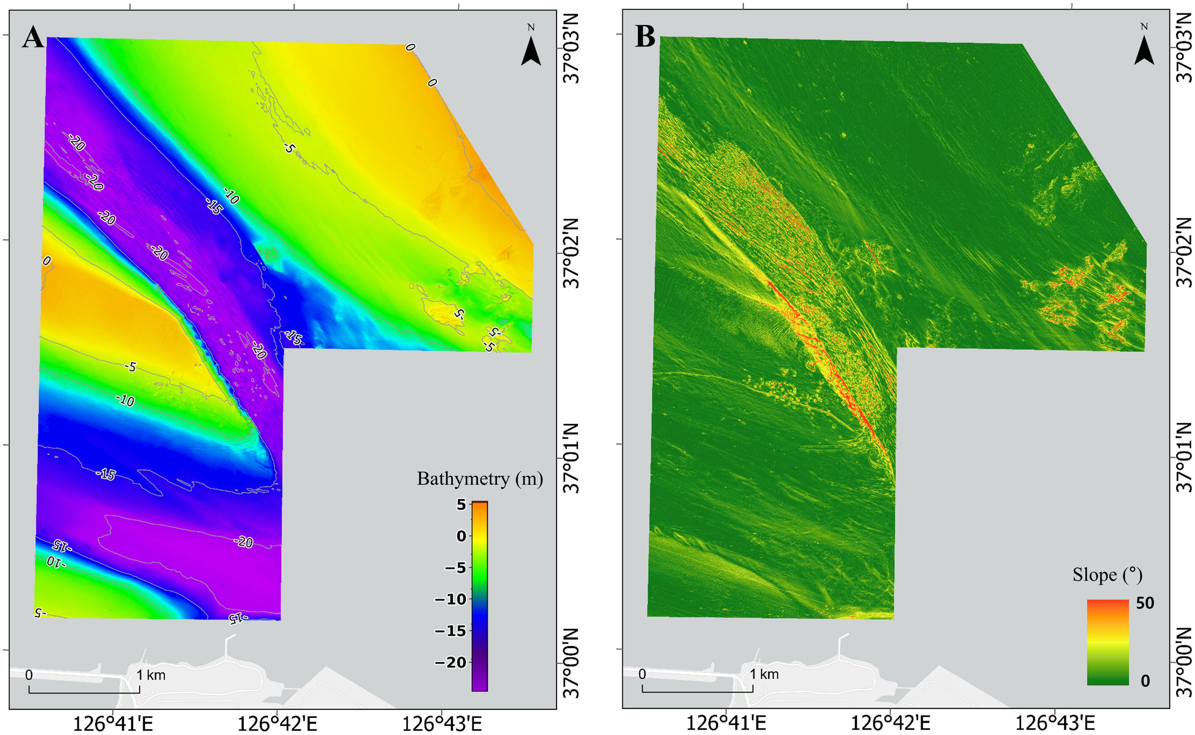
Figure 2. (A) Bathymetric digital elevation model (DEM) of the study area derived from multibeam echo sounder data. The raster is presented at a spatial resolution of 1 m × 1 m. Color shading follows a perceptually uniform colormap, where lighter tones indicate shallower areas and darker tones represent deeper regions. (B) Seafloor slope distribution calculated from the bathymetric surface, expressed in degrees. Steeper slopes are observed along tidal channel margins, while gentler slopes dominate the central shoal and intertidal flats.

Multispectral backscatter mosaics at 170, 300, and 450 kHz show distinct differences in acoustic intensity across frequencies (Figures 3A–C). Regions of low backscatter intensity were consistently identified at all frequencies, while higher-intensity zones agreed spatially with topographic features identified in the bathymetric data. The backscatter intensity range widened with decreasing frequency, with the maximum contrast observed between the 170 and 450 kHz datasets. Quantitative analysis showed a maximum difference of 18.29 dB in the average backscatter intensity between 170 and 450 kHz in selected high-contrast zones.

Figure 3

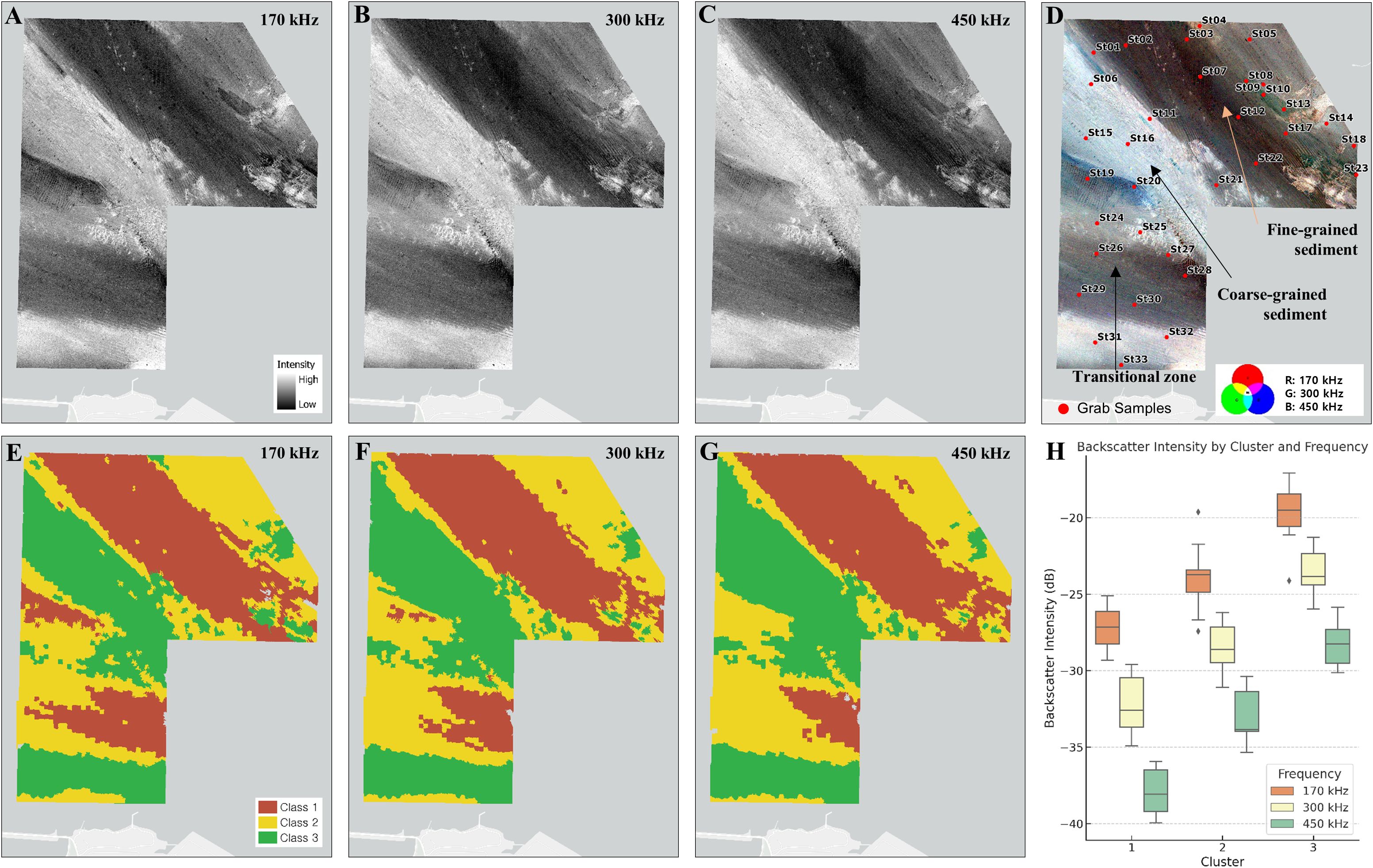
Figure 3. Backscatter intensity mosaics acquired at (A) 170, (B) 300, and (C) 450 kHz. Grayscale shading represents the relative acoustic backscatter strength, where brighter tones indicate higher intensities and darker tones indicate weaker returns. (D) Red–green–blue (RGB) composite image of the three frequency backscatter mosaics (red = 170 kHz, green = 300 kHz, and blue = 450 kHz). Markings indicate key sediment zones, coarse-grained (blue), fine-grained (gray/red), and transitional (mixed), to clarify the relationship between color patterns and sediment types. K-means clustering results based on the backscatter intensity at (E) 170, (F) 300, and (G) 450 kHz. Cluster colors are assigned independently per frequency for visualization purposes. (H) Box plots showing the statistical distributions of backscatter intensity by class and frequency.

An RGB composite image constructed from the three frequency-specific backscatter mosaics (red = 170 kHz, green = 300 kHz, and blue = 450 kHz) highlighted spatial variation in the multispectral acoustic response (Figure 3D). In the RGB composite, zones with stronger returns (450 kHz) showed predominantly blue to purple hues, whereas higher-intensity areas (170 kHz) were more reddish. These results qualitatively reflect spatial variation in the frequency-dependent acoustic response.

3.2 Multifrequency backscatter intensity and sediment classification of the seabed

The K-means clustering results, applied separately to each frequency, identified three dominant acoustic classes per frequency (Figures 3E–G). The spatial distribution of these classes varied among frequencies, reflecting differences in the seabed acoustic response characteristics. These classifications corresponded to the observed bathymetric patterns, including steep channel slopes, flat shoals, and nearshore platforms. Statistical analysis showed a clear trend, with backscatter intensity decreasing with increasing frequency. Differences in backscatter intensity between classes exhibited distinct patterns depending on the applied frequency (Figure 3H).

At 170 kHz, class 1 had the lowest mean backscatter intensity at –27.26 dB (standard deviation [SD] = 1.43 dB), while classes 2 and 3 had progressively higher values of –23.95 dB (SD = 2.09 dB) and –19.67 dB (SD = 2.12 dB), respectively. Notably, class 3 had the strongest acoustic reflection, with a maximum intensity of –17.09 dB. The relatively high variability within class 3 suggests a diverse composition of sediment types.

At 300 kHz, a general reduction in backscatter intensity was observed. Class 1 had the weakest reflection (–32.35 dB, SD = 1.88 dB), followed by class 2 (–28.58 dB, SD = 1.62 dB), and class 3, which had the highest response (–23.48 dB, SD = 1.54 dB), with a maximum intensity of –21.27 dB. The difference in mean intensity between classes 1 and 3 was approximately 8.87 dB, reinforcing the distinct acoustic signatures of sediment types at this frequency.

More pronounced attenuation in backscatter intensity was observed at a frequency of 450 kHz. Class 1 had the lowest mean value at –37.96 dB (SD = 1.50 dB), while classes 2 and 3 measured –33.11 dB (SD = 1.59 dB) and –28.25 dB (SD = 1.39 dB), respectively. Again, class 3 had the strongest maximum intensity at –25.87 dB. Class 2 had the highest SD, indicating greater sediment heterogeneity.

Class 3 consistently had the highest backscatter intensity across all frequencies, indicating coarse-grained sediments or high-density substrates. Conversely, class 1 consistently had the weakest backscatter intensity, reflecting fine, organic-rich sediment. The consistent decrease in backscatter intensity with increasing frequency aligns with the expected trend of frequency-dependent acoustic response behavior.

3.3 Characterization of sediment classes using ground-truth data

Thirty-three grab samples were used to validate the acoustically defined sediment classification derived from the multifrequency backscatter and bathymetric data. Clustering separated the seabed into three acoustic classes, which were systematically compared to ground-truth sediment properties, such as grain size distribution, total organic carbon (TOC), water content, backscatter strength (BS), slope, and sediment facies (Table 2; Figure 4).

Table 2

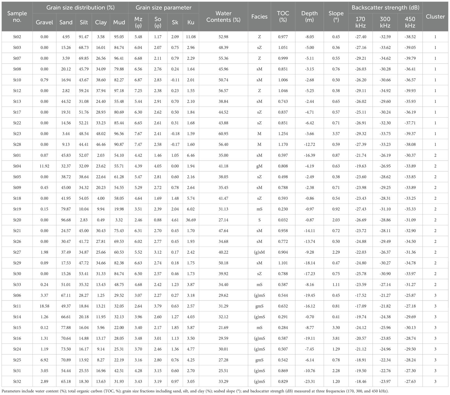
Table 2. Summary statistics of sediment properties for three acoustic sediment classes, validated using 33 ground-truth grab samples.

Figure 4

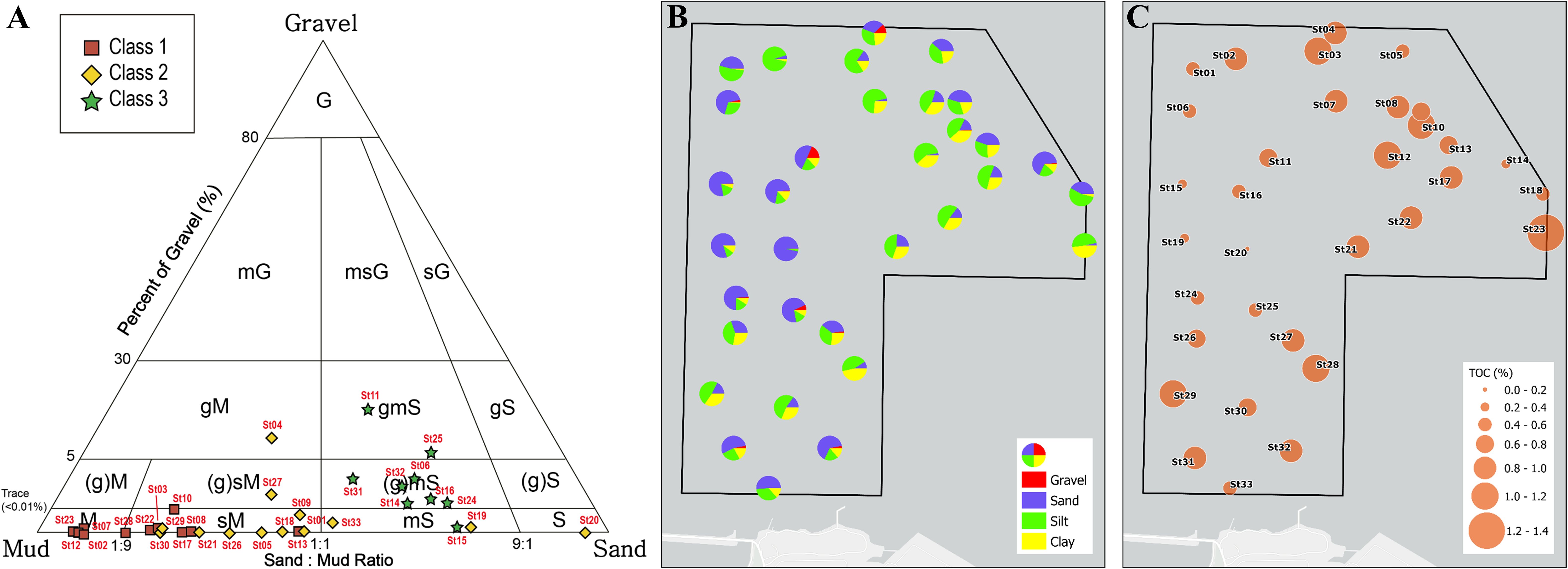
Figure 4. (A) Ternary diagram of grain size distribution (gravel, sand, and mud) for grab samples, with each data point color-coded according to its acoustic class as defined by clustering analysis of multifrequency backscatter data. Class 1 samples are clustered near the mud-dominated apex, class 3 samples are near the sand-rich corner, and class 2 samples occupy intermediate positions, indicating compositional transitions. (B) Station-specific pie charts showing the measured proportions of gravel, sand, silt, and clay at each grab sampling location. These charts present only the actual grain size composition at each station and are independent of the acoustic class assignment. (C) Spatial distribution of total organic carbon (TOC) interpolated across the study area. Higher TOC values are concentrated in class 1 regions, whereas lower values corresponded to sandier class 3 zones, consistent with the sediment classification framework.

Class 1 was characterized by fine-grained sediments with high water and organic contents. The mud content (silt + clay) averaged 85.87%, and individual samples often exceeded 90%, while the sand content remained low (mean = 14.06%). This class had the highest water content among all groups, with an average of 50.42% and maximum of 60.95%. TOC values followed a similar trend, with a mean of 0.98% and a maximum of 1.25%. The low-energy, fine-grained nature of class 1 was further reflected in the acoustic and slope data; the average backscatter strength ranged from –25.11 dB (170 kHz) to –37.96 dB (450 kHz), and the slopes were the lowest overall, averaging 0.83° (SD = 0.92°). Sediment facies observed within this class were dominated by Z (silt), sZ (sandy silt), sM (sandy mud), and M (mud) types.

Class 2 had greater sediment heterogeneity. The mud content ranged from 3.32% to 84.74% (mean = 56.03%), while the sand content ranged from 15.26% to 96.68% (mean = 42.83%), indicating transitional textures. The water content averaged 38.19%, while TOC concentrations were lower than in class 1 (mean = 0.67%), but showed considerable variability (0.03–1.10%). Class 2 had an intermediate acoustic response, with backscatter intensities averaging –23.95 dB (170 kHz), –28.58 dB (300 kHz), and –33.11 dB (450 kHz). The mean slope was 0.92°, slightly higher than in class 1, but markedly lower than in class 3. The observed facies types included sZ, sM, slightly gravelly sandy mud [(g)sM], gravelly mud (gM), muddy sand (mS), and sand (S), reflecting a mixture of depositional energies.

Class 3 contained the coarsest, most acoustically reflective sediments. The average sand content was 66.18%, with several samples exceeding 75%, and gravel was present at multiple stations. The mud content was markedly lower (mean = 29.52%), and the water content also declined, with an average of 28.93% and minimum of 21.69%. TOC values were the lowest overall, averaging 0.57% and dropping to 0.28% in the coarsest samples. The backscatter strength in class 3 was consistently high across all frequencies (–19.67 dB at 170 kHz, –23.48 dB at 300 kHz, and –28.25 dB at 450 kHz), and the slope was the steepest among all classes (mean = 1.59°, maximum = 3.81°, SD = 1.25°). The sediment facies predominantly consisted of mS, gravelly muddy sand (gmS), and (g)mS, aligning with the coarser grain sizes.

The distribution of sediment classes was supported by ternary grain size diagrams (Figure 4A), the station-specific grain composition (Figure 4B), and spatial TOC variation (Figure 4C). Class 1 stations clustered within the mud-dominant apex of the ternary plot, whereas class 3 occupied the sand-rich domain, with class 2 distributed between these endmembers. While there is a strong correspondence between acoustic classes and sediment texture, the acoustic classes are based on similarities in acoustic response and do not correspond directly to the traditional grain size categories.

4 Discussion

4.1 Advantages of multifrequency backscatter in sediment classification

This study demonstrated that multifrequency acoustic backscatter analysis improves seabed sediment differentiation, complementing limitations of traditional single-frequency methods (Feldens et al., 2018; Brown et al., 2019; Runya et al., 2021). Conventional single-frequency surveys rely primarily on acoustic intensity variation at a single wavelength, which is often insufficient for resolving complex sedimentary environments where multiple factors such as grain size, surface roughness, sediment density, and organic matter content influence the acoustic scattering simultaneously (Goff et al., 2000; Moore et al., 2013; Brown et al., 2019). By combining multiple frequencies in this study (170, 300, and 450 kHz), we leveraged their distinct acoustic responses, thereby significantly enhancing sediment classification accuracy.

Each frequency contributes differently to the characterization of sediment properties (Figures 3A–C). Lower frequencies such as 170 kHz effectively capture signals from below the immediate seabed surface, making them useful for detecting sediment layering, buried structures, or variation in sediment composition beneath the surface. Intermediate frequencies (e.g., 300 kHz) offer balanced insights into both surface properties and shallow subsurface sediment features, and offer versatility for general sediment classification purposes. Higher frequencies (e.g., 450 kHz), are highly sensitive to surface roughness, sediment compaction, and grain-scale textural differences, making them ideal for detecting coarse-grained sediments, gravelly substrates, or areas with marked surface irregularities (Gaida et al., 2019).

In this study, the maximum observed difference in acoustic intensity between 170 and 450 kHz was 18.29 dB, reflecting substantial variability in sediment surface properties and scattering mechanisms (Figures 3A, C). This 18.29-dB difference indicates a clear distinction in the acoustic responses of sediments at different penetration depths and surface roughness scales. For example, sediments with lower intensities at 450 kHz relative to 170 kHz suggest smoother, fine-grained surfaces or increased acoustic absorption at the seabed–water interface. Conversely, sediments with higher intensities at 450 kHz than at 170 kHz indicate the presence of coarser-grained substrates, pronounced surface roughness, or densely compacted sediment layers with limited acoustic penetration. Thus, a large decibel difference across these frequencies provides useful diagnostic cues for distinguishing sediment types, particularly in transitional or heterogeneous seabed areas.

Integrating these frequencies into RGB composite images (170 kHz as red, 300 kHz as green, and 450 kHz as blue) enabled intuitive visual differentiation of sedimentary environments (Figure 3D). High-frequency returns (450 kHz), prominently displayed in blue, effectively highlighted areas of coarse-grained or rough-surface sediments (Figure 3C). By contrast, dominant low-frequency (170 kHz) reflections, depicted in reddish tones, emphasized sediment features influenced by buried layers or subsurface compositional differences (Figure 3A). Consequently, transitional sediment zones or mixed sediment environments, which are often ambiguous in single-frequency backscatter images, were delineated effectively (Figure 3D).

Applying multifrequency backscatter data in clustering algorithms such as the K-means algorithm substantially improved the classification accuracy. Simultaneous consideration of frequency-specific responses allowed sediment classes defined by distinct grain sizes, surface textures, and densities to be separated accurately. This multifrequency approach significantly enhanced the mapping and interpretation of complex seabed environments, improving confidence in sedimentological assessments (Frederick et al., 2020; Menandro et al., 2022, 2025).

4.2 Interpretation of sediment class characteristics

The interpretation presented in this section is based on a unified sediment classification scheme derived from clustering analysis that simultaneously incorporates backscatter intensity data from three frequencies: 170, 300, and 450 kHz. Rather than treating each frequency independently, the classification process used a multi-dimensional input vector for each station (i.e., [BS170, BS300, and BS450]) as multi-dimensional input for the K-means clustering algorithm. This approach yielded a single set of three sediment classes, whose physical and geochemical characteristics were validated using ground-truth sample analyses (Table 2) and interpreted in relation to spatial patterns (Figures 2-4).

Note that the classification maps shown in Figures 3E–G represent frequency-specific clustering results derived from 170, 300, and 450 kHz backscatter data, respectively. These maps illustrate the spectral variability across frequencies. However, the sediment classification interpreted in this section is based on a unified clustering model that simultaneously incorporated all three frequencies. The resulting integrated classification is presented in Table 3 and subsequent sedimentological interpretations.

Table 3

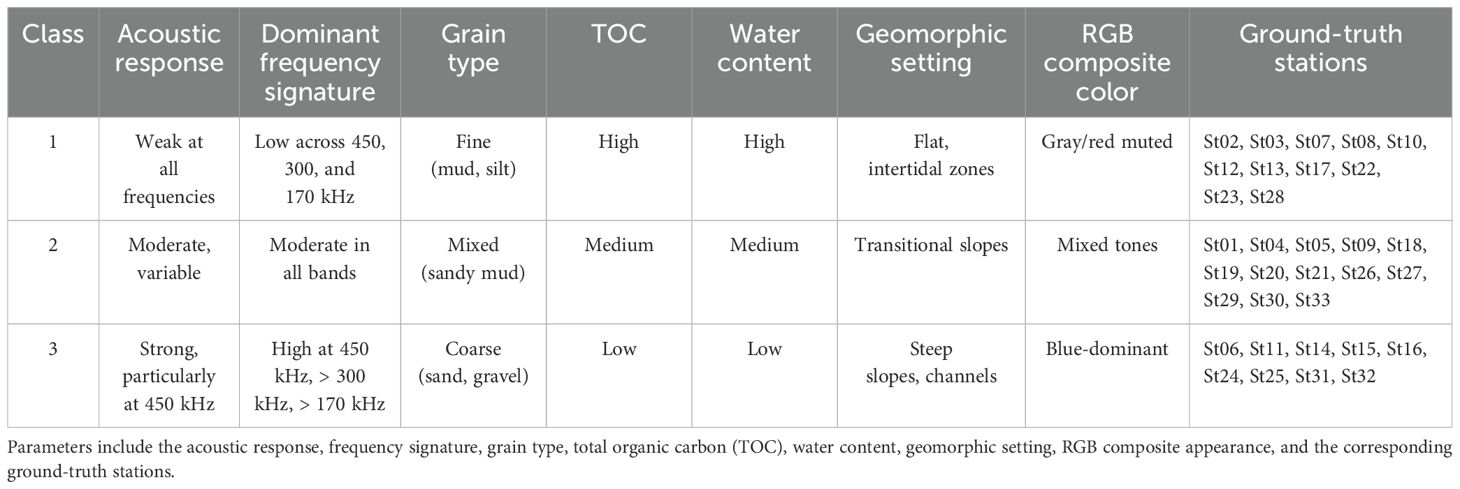
Table 3. Key sediment characteristics for classes 1–3 derived from integrated multi-frequency backscatter classification.

Class 1 was associated with acoustically weak returns across all frequencies and matched ground-truth samples with fine-grained textures, high water content, and elevated TOC. These properties are characteristic of low-energy depositional environments, such as intertidal flats or protected shoal zones. The facies types in this class were dominated by mud-rich categories (e.g., Z, sZ, sM, and M), reflecting stable, organic-rich sediments. In the RGB composites, these areas showed as muted or blended color tones, consistent with uniformly low acoustic intensity (Figure 3D).

By contrast, class 3 showed strong acoustic returns, particularly at higher frequencies, and corresponded to sediments with coarse textures, low organic content, and minimal moisture. This class was frequently located along steeper slopes and channel flanks (Figure 2B), suggesting the influence of hydrodynamic processes. The facies types observed in class 3 (e.g., mS, gmS, and (g)mS) supported the interpretation of energetic depositional conditions. In the RGB image, these areas were visually distinct with blue-dominated tones due to enhanced reflectivity at 450 kHz.

Class 2 was intermediate between classes 1 and 3, both acoustically and sedimentologically. It showed moderate backscatter values and a wide range of grain size compositions. Spatially, class 2 was often observed at transitional boundaries between muddy flats and coarser channel margins, likely reflecting reworked or mixed sediment conditions. Its facies diversity, including mS, gmS, and (g)mS, confirmed its heterogeneity.

The correspondence between the multifrequency acoustic response and ground-truth sediment properties illustrates the strength of the integrated classification approach. This method effectively distinguished textural endmembers and transitional sediment regimes, which are commonly ambiguous in single-frequency analyses (Feldens et al., 2018; Schulze et al., 2022). The spatial consistency of the acoustic classes with underlying geomorphological (Figure 2) and sedimentological attributes (Figures 3, 4) reinforces the reliability of this classification for interpreting complex seabed conditions.

The observed spatial distribution of sediment classes closely reflects the geomorphological and hydrodynamic setting of Asan Bay (Figure 1). The central sand ridge and adjacent tidal channels, characterized by greater depths (16–20 m), persistent submergence, and stronger tidal currents, are dominated by coarse-grained sediments (class 3), as confirmed by ground-truth samples and the blue-dominated zones in the acoustic composites (Figure 3D). The high-energy tidal flows in these areas promote winnowing, resuspension, and the persistence of sand-rich substrates. In contrast, the shallower intertidal flats (4–6 m) along the bay’s margin, which experience weaker currents and periodic exposure at low tide, are dominated by fine-grained, mud-rich sediments (class 1), as indicated by low acoustic intensity and the prevalence of Z, sZ, sM, and M facies. Class 2, often occurring at the transitional boundaries between the sand ridge and tidal flats, reflects mixed or reworked conditions shaped by fluctuating current strengths and sediment supply. The overall sediment distribution thus emerges from the interplay of local bathymetry, tidal energy gradients, and restricted fluvial input due to dammed rivers and seawalls. These findings underscore the strong coupling between geomorphological structure, hydrodynamic regime, and the resulting sedimentary facies patterns in Asan Bay.

4.3 Limitations and future perspectives

Despite the clear advantages of multifrequency acoustic backscatter methods, several practical limitations require careful consideration. One challenge is the ambiguity arising from overlapping acoustic responses driven by multiple sedimentary factors, i.e., grain size, sediment density, porosity, organic content, and surface roughness, which simultaneously influence the acoustic scattering. While the multifrequency statistical analyses presented in this study demonstrate frequency-dependent acoustic variability associated with sediment properties (see Sections 4.1 and 4.2; Table 2, Figure 3), precisely quantifying the contribution of each property remains difficult. For example, high backscatter intensities observed consistently for class 3 across frequencies suggest coarse sediment composition and higher density or compactness, yet within-class variation indicates the presence of mixed sediment types or heterogeneity in subsurface structures. At lower frequencies (170 kHz), substantial variability (class 3, SD = 3.26 dB) implies complexity due to internal sedimentary layering or exposed consolidated substrates.

Another limitation involves subjectivity, which is evident when visually interpreting RGB composite images (Figure 3D) or making manual clustering decisions. Although this study employed the K-means algorithm, which offers a reproducible and statistically objective framework for clustering, its outcomes can be affected by factors such as the choice of initial centroids, the preset number of clusters (k), and the assumption of spherical cluster boundaries. Moreover, K-means may be limited in detecting non-linear or complex relationships present in heterogeneous sedimentary environments. To further enhance objectivity and classification performance, advanced machine learning techniques, such as random forests, support vector machines, or convolutional neural networks, could be applied in future research. These approaches have the potential to integrate multivariate acoustic and environmental data, recognize subtle sedimentary patterns, and reduce human bias through more flexible, data-driven modeling. However, their effective implementation requires extensive, well-labeled datasets and robust model validation, which were beyond the scope of the present study. Nevertheless, the combination of objective clustering and independent ground-truthing adopted here provides a robust basis for acoustic sediment classification in this setting.

Sediment surface characteristics, such as biofilms, bioturbation, and macrofaunal activity, can also alter acoustic scattering, particularly at higher frequencies sensitive to surface texture. Such temporal biological dynamics can modify surface roughness or biofilm layers, potentially masking sedimentary signals and introducing variability in backscatter measurements over time. Incorporating repeated seasonal sampling, sediment cores, and in situ optical imaging may help to account for these transient features and refine interpretations.

The frequencies used in this study (170, 300, and 450 kHz) offered a useful balance between resolution and penetration depth. However, the inclusion of additional frequency bands below 100 kHz or above 500 kHz could improve vertical sediment discrimination or surface texture resolution, respectively (Gaida et al., 2018; Runya et al., 2021; Menandro et al., 2022; Bai et al., 2023). Combining multifrequency backscatter data with sub-bottom profiling tools (e.g., chirp sonar) could enable more effective delineation of buried sediment layers and detection of sediment accumulation sequences. Furthermore, coupling multifrequency acoustic datasets with geochemical and geotechnical sediment analyses could enhance the interpretation and provide a more comprehensive view of sedimentary dynamics.

Importantly, the multifrequency acoustic classification method used in this study is based on well-established physical principles and standard corrections for water depth, transmission loss, incidence angle, and environmental factors such as temperature and salinity. Previous studies have shown that, after such corrections, backscattering strength is generally high for coarse-grained sediments and low for fine-grained sediments, regardless of water depth or seabed morphology (Gaida et al., 2018; Lamarche and Lurton, 2018; Bai et al., 2023). As summarized in Table 3, our results conform to these widely recognized patterns: class 3 is dominated by coarse-grained sediments with high backscatter strength, while class 1 is characterized by fine-grained sediments and lower backscatter values. These findings support the applicability and generalizability of our approach across different water depths, sediment grain sizes, and complex seabed terrains.

The observed acoustic variability and classification uncertainties highlight the need for future research to address the multidimensional variability of acoustic responses, optimize frequency selection for site-specific applications, and expand classification approaches by integrating physically informed acoustic scattering models and supervised machine learning frameworks that incorporate not only backscatter data but also morphological and sediment core information.

5 Conclusions

This study demonstrated that integrating multifrequency multibeam backscatter data enhances the classification and interpretation of seabed sediment characteristics in complex coastal environments. The method was shown to be robust across varying water depths, sediment grain-size compositions, and heterogeneous seabed terrains, supporting its general applicability to a range of dynamic marine settings. By analyzing acoustic responses at 170, 300, and 450 kHz, distinct frequency-dependent backscatter patterns were observed, allowing improved discrimination of sediment textures and structures that are often ambiguous in single-frequency surveys. Notably, RGB composite imagery and spectral clustering approaches effectively visualized and differentiated transitional sediment zones. These results are in line with recent advances in multifrequency MBES research, further validating the reliability of the approach.

A unified classification framework incorporating backscatter intensities from all three frequencies successfully identified three sediment classes: class 1 (fine-grained, organic-rich), class 2 (mixed textures), and class 3 (coarse-grained, compacted). Ground-truth validation using grab samples confirmed that these classes consistently corresponded with grain size distribution, water content, TOC, slope, and sediment facies. The spatial distribution of sediment classes was strongly linked to underlying geomorphological features and local hydrodynamic conditions, demonstrating the influence of topography and tidal currents on sedimentary processes. This alignment underscores the reliability of the multifrequency classification in reflecting physical and geochemical seabed properties.

While the present approach offers considerable improvements in resolution and accuracy, challenges remain in decoupling the acoustic influences of overlapping sediment parameters and addressing potential subjectivity in RGB interpretation. Future research should explore expanded frequency ranges, machine learning-based classification models, and integration with sub-bottom and geochemical data to advance sediment mapping capabilities.

Our results provide a robust foundation for high-resolution seabed characterization and support applications in benthic habitat assessment, sediment transport analysis, and coastal resource management.

Data availability statement

The original contributions presented in the study are included in the article/supplementary material. Further inquiries can be directed to the corresponding author.

Author contributions

ML: Writing – review & editing, Writing – original draft, Project administration. JKA: Writing – review & editing, Project administration, Writing – original draft. SH: Software, Writing – review & editing. EJ: Methodology, Writing – review & editing. B-CK: Resources, Writing – review & editing. JKU: Investigation, Methodology, Resources, Writing – review & editing.

Funding

The author(s) declare that financial support was received for the research and/or publication of this article. This research was supported by the Korea Institute of Marine Science & Technology Promotion (KIMST), funded by the Ministry of Oceans and Fisheries (RS-2022-KS221578), and by the Korea Institute of Ocean Science & Technology (PEA0333).

Acknowledgments

The acquisition of seafloor topography and backscattered sound pressure data was made possible through the assistance of the KHOA.

Conflict of interest

The authors declare that the research was conducted in the absence of any commercial or financial relationships that could be construed as a potential conflict of interest.

Generative AI statement

The author(s) declare that no Generative AI was used in the creation of this manuscript.

Publisher’s note

All claims expressed in this article are solely those of the authors and do not necessarily represent those of their affiliated organizations, or those of the publisher, the editors and the reviewers. Any product that may be evaluated in this article, or claim that may be made by its manufacturer, is not guaranteed or endorsed by the publisher.

References

Augustin J. M., Le Suave R., Lurton X., Voisset M., Dugelay S., and Satra C. (1996). Contributions of the multibeam acoustic imagery to the exploration of the seabottom. Mar. Geophys. Res. 18, 459–486. doi: 10.1007/BF00286090

Crossref Full Text | Google Scholar

Bai Q., Mestdagh S., Snellen M., and Amiri-Simkooei A. (2023). “Characterizing seabed sediments using multi-spectral backscatter data in the North Sea,” in OCEANS 2023-Limerick (Ireland: IEEE), 1–7.

Google Scholar

Ball G. H. and Hall D. J. (1965). ISODATA: a novel method of data analysis and pattern classification (Menlo Park, CA: Stanford Research Institute International).

Google Scholar

Bang K. Y., Park S. J., Kim S. O., Cho C. W., Kim T. I., Song Y. S., et al. (2013). Numerical hydrodynamic modeling incorporating the flow through permeable Sea-wall. J. Korean Soc. Coast. Ocean Engineers 25, 63–75. doi: 10.9765/KSCOE.2013.25.2.63

Crossref Full Text | Google Scholar

Brown C. J., Beaudoin J., Brissette M., and Gazzola V. (2019). Multispectral multibeam echo sounder backscatter as a tool for improved seafloor characterization. Geosciences 9, 126. doi: 10.3390/geosciences9030126

Crossref Full Text | Google Scholar

Chang T. S. and Nam S. I. (2011). Geochemical logging of shallow-sea tidal bar sediment cores using a XRF core scanner: an application of XRF core-scanning to lithostratigraphic analysis. J. Geo. Soc Korea 47, 471–485.

Google Scholar

Eleftherakis D., Amiri-Simkooei A., Snellen M., and Simons D. G. (2012). Improving riverbed sediment classification using backscatter and depth residual features of multi-beam echo-sounder systems. J. Acoust. Soc Am. 131, 3710–3725. doi: 10.1121/1.3699206

PubMed Abstract | Crossref Full Text | Google Scholar

Feldens P., Schulze I., Papenmeier S., Sch€onke M., and Schneider von Deimling J. (2018). Improved interpretation of marine sedimentary environments using multi-frequency multibeam backscatter data. Geosciences 8, 214. doi: 10.3390/geosciences8060214

Crossref Full Text | Google Scholar

Fezzani R., Berger L., Le Bouffant N., Fonseca L., and Lurton X. (2021). Multispectral and multiangle measurements of acoustic seabed backscatter acquired with a tilted calibrated echosounder. J. Acoust. Soc Am. 149, 4503–4515. doi: 10.1121/10.0005428

PubMed Abstract | Crossref Full Text | Google Scholar

Folk R. (1974). Petrology of Sedimentary Rocks (Austin, USA: Hemphills Publishing).

Google Scholar

Frederick C., Villar S., and Michalopoulou Z. H. (2020). Seabed classification using physics-based modeling and machine learning. J. Acoust. Soc Am. 148, 859–872. doi: 10.1121/10.0001728

PubMed Abstract | Crossref Full Text | Google Scholar

Gaida T. C., Ali T. A. T., Snellen M., Simkooei A. A., van Dijk T. A. G. P., and Simons D. G. (2018). A multispectral bayesian classification method for increased acoustic discrimination of seabed sediments using multi-frequency multibeam backscatter data. Geosciences 8, 455. doi: 10.3390/geosciences8120455

Crossref Full Text | Google Scholar

Gaida T. C., Mohammadloo T. H., Snellen M., and Simons D. G. (2019). Mapping the seabed and shallow subsurface with multi-frequency multibeam echosounders. Remote Sens. 12, 52. doi: 10.3390/rs12010052

Crossref Full Text | Google Scholar

Galehouse J. S. (1971). Sedimentation analysis. Procedures in sedimentary petrology (New York: Wiley Interscience), 69–94.

Google Scholar

Gavrilov A. N., Siwabessy P. J. W., and Parnum I. M. (2005). Multibeam echo sounder backscatter analysis (Curtin University of Technology).

Google Scholar

Goff J. A., Olson H. C., and Duncan C. S. (2000). Correlation of side-scan backscatter intensity with grain-size distribution of shelf sediments, New Jersey margin. Geo-Mar. Lett. 20, 43–49. doi: 10.1007/s003670000032

Crossref Full Text | Google Scholar

Ingram R. (1971). Sieve analysis. Procedures in sedimentary petrology (New York: Wiley Interscience), 49–67.

Google Scholar

Jeong Y. H., Cho M. K., Lee D. G., Doo S. M., Choi H. S., and Yang J. S. (2016). Seasonal variations in seawater quality due to freshwater discharge in Asan bay. J. Korean Soc Mar. Environ. Saf. 22, 454–467. doi: 10.7837/kosomes.2016.22.5.454

Crossref Full Text | Google Scholar

Kågesten G. and Bengt L. (2008). Geological seafloor mapping with backscatter data from a multibeam echo sounder (Gothenburg, Sweden: Department of Earth Sciences, Gothenburg University).

Google Scholar

Khomsin M., Pratomo D. G., and Suntoyo (2021). The development of seabed sediment mapping methods: the opportunity application in the coastal waters. IOP Conf. Ser.: Earth Environ. Sci. 731, 12–39. doi: 10.1088/1755-1315/731/1/012039

Crossref Full Text | Google Scholar

Korea Hydrographic and Oceanographic Agency (KHOA) (2008). Jungangcheontoe Sand Bar in Macrotidal Channel of outer Asan Bay, Korea. Korea: Korea Hydrographic and Oceanographic Agency.

Google Scholar

Korea Hydrographic and Oceanographic Agency (KHOA) (2009). Study on submarine topographic changes of the Kyunggi Bay in the Yellow Sea: Jungangcheontoe in Asan Bay.

Google Scholar

Lamarche G. and Lurton X. (2018). Recommendations for improved and coherent acquisition and processing of backscatter data from seafloor-mapping sonars. Mar. Geophys. Res. 39, 5–22. doi: 10.1007/s11001-017-9315-6

Crossref Full Text | Google Scholar

Lurton X., Lamarche G., Brown C., Lucieer V., Rice G., Schimel A., et al. (2015). Backscatter measurements by seafloor-mapping sonars. Guidelines Recom. (Version 1.0). doi: 10.5281/ZENODO.10089261

Crossref Full Text | Google Scholar

Malik M. (2019). Estimation of Measurement Uncertainty of Seafloor Acoustic Backscatter (University of New Hampshire).

Google Scholar

McManus J. (1988). “Grain size determination and interpretation,” in Techniques in sedimentology. Ed. Tucker M. E. (Blackwell, Oxford), 63–85.

Google Scholar

Menandro P. S., Bastos A. C., Misiuk B., and Brown C. J. (2022). Applying a multi-method framework to analyze the multispectral acoustic response of the seafloor. Front. Remote Sens 3, 860282. doi: 10.3389/frsen.2022.860282

Crossref Full Text | Google Scholar

Menandro P. S., Misiuk B., Schneider von Deimling J., Bastos A. C., and Brown C. J. (2025). Multifrequency seafloor acoustic backscatter as a tool for improved biological and geological assessments–updating knowledge, prospects, and challenges. Front. Remote Sens. 6, 1546280. doi: 10.3389/frsen.2025.1546280

Crossref Full Text | Google Scholar

Misiuk B., Tan Y. L., Li M. Z., Trappenberg T., Alleosfour A., Church I. W., et al. (2024). Multivariate mapping of seabed grain size parameters in the Bay of Fundy using convolutional neural networks. Mar. Geol. 472, 107299. doi: 10.1016/j.margeo.2024.107299

Crossref Full Text | Google Scholar

Moore S. A., Le Coz J., Hurther D., and Paquier A. (2013). Using multi-frequency acoustic attenuation to monitor grain size and concentration of suspended sediment in rivers. J. Acoust. Soc Am. 133, 1959–1970. doi: 10.1121/1.4792645

PubMed Abstract | Crossref Full Text | Google Scholar

R2Sonic (2017). SONIC 2026/2024/2022 BROADBAND MULTIBEAM ECHOSOUNDERS Operation Manual V6.3.

Google Scholar

Runya R. M., McGonigle C., Quinn R., Howe J., Collier J., Fox C., et al. (2021). Examining the links between multi-frequency multibeam backscatter data and sediment grain size. Remote Sens. 13, 1539. doi: 10.3390/rs13081539

Crossref Full Text | Google Scholar

Schimel A. C., Beaudoin J., Parnum I. M., Le Bas T., Schmidt V., Keith G., et al. (2018). Multibeam sonar backscatter data processing. Mar. Geophys. Res. 39, 121–137. doi: 10.1007/s11001-018-9341-z

Crossref Full Text | Google Scholar

Schulze I., Gogina M., Schönke M., Zettler M. L., and Feldens P. (2022). Seasonal change of multifrequency backscatter in three Baltic Sea habitats. Front. Remote Sens. 3, 956994. doi: 10.3389/frsen.2022.956994

Crossref Full Text | Google Scholar

Simons D. G. and Snellen M. (2009). A Bayesian approach to seafloor classification using multibeam echo-sounder backscatter data. Appl. Acoust 70, 1258–1268. doi: 10.1016/j.apacoust.2008.07.013

Crossref Full Text | Google Scholar

Wildish D. J., Hughes Clarke J. E., Pohle G. W., Hargrave B. T., and Mayer L. M. (2004). Acoustic detection of organic enrichment in sediments at a salmon farm is confirmed by independent groundtruthing methods. Mar. Ecol. Prog. Ser. 267, 99–105. doi: 10.3354/meps267099

Crossref Full Text | Google Scholar

Zhou Q., Li X., Liu L., Wang J., Zhang L., and Liu B. (2023). Classification of seafloor sediment in northern slope of South China sea based on improved U-net and K-means clustering analysis. Remote Sens. 15 (14), 3576. doi: 10.20944/preprints202305.2240.v1

Crossref Full Text | Google Scholar