FS-STFNet: a few-shot adaptive spatiotemporal fusion network for short-term tropical cyclone intensity forecasting

Tropical cyclone (TC) intensity prediction is a critical task in disaster prevention and mitigation. Due to the high complexity and incomplete evolution mechanism, the accurate prediction of TC intensity remains a challenge. This study proposes a Few-Shot Spatiotemporal Fusion Network (FS-STFNet) to improve short-term TC intensity prediction under limited data. A spatial enhancement module is designed to adaptively fuse and enhance features from multi-source data (i.e. trajectories, atmospheric reanalysis, and satellite imagery). Then, an autoregressive deep learning model with enhanced spatiotemporal transformation equation is designed for short-term intensity prediction of single TC without relying large number of temporal training samples. A test applying the FS-STFNet to TCs in Northwest Pacific from 2019 to 2021 demonstrate the effectiveness and superiority compared to other methods. The model achieves optimal performance during stable TCs structures while effectively reducing biases for weak TCs or topography-affected cases through adaptive adjustments. This work offers a scalable technical framework for extreme weather forecasting in temporal data-scarce scenarios, supporting disaster preparedness.

1 Introduction

Tropical cyclones (TCs) are low-pressure weather systems characterized by strong sudden onset and destructive power. They primarily manifest as powerful winds, heavy rainfall, storm surges, and geological disasters (Zhang et al., 2022). As one of the most severe natural disasters affecting human activities, TCs have become a significant factor limiting the sustainable development of society and economy (Xing et al., 2011). Therefore, accurate forecasting of TCs intensity is crucial for disaster prevention and mitigation. Timely warning of TCs not only helps minimize risks but also plays a crucial role in enabling a swift response and the implementation of effective rescue operations.

Traditional TCs intensity forecasting methods are primarily based on Numerical Weather Prediction (NWP) models, which simulate atmospheric processes by solving atmospheric dynamics and thermodynamics equations to predict the evolution of TCs (Huang et al., 2011). With the advancement of computer technology and supercomputing, numerical forecasting methods have been widely applied to TCs intensity prediction, achieving significant progress (Bauer et al., 2015). Existing numerical prediction models, are capable of simulating TCs tracks with reasonable accuracy. However, there remains significant uncertainty in predicting their intensity, traditional numerical models often struggle to provide accurate forecasts due to limitations in initial conditions and the parameterization of physical processes. In addition, numerical models are time consuming. High-resolution numerical analysis of TCs may take several hours, which is one of the reasons why most official cyclone forecasts are issued every 6 hours (Xu et al., 2013).

In recent years, with the explosive growth of multi-source monitoring data, data-driven methods have been successfully developed in various fields by extracting features within large datasets (LeCun et al., 2015). In view of that the study of the physical mechanism involved in TCs is difficult to achieve great breakthroughs in a short period of time, some researchers tried to improve TC intensity prediction based on deep learning methods. For example, a neural network framework was designed to achieve fine-grained TC intensity prediction based on multi-source environmental variables (Zhang et al., 2022); Xu et al. proposed a spatial attention fusing network for TC intensity prediction. The model combined both 2D and 3D typhoon structure domain-expert knowledge (Xu et al., 2022). Huang et al. proposed TropiCycloneNet, a dual-perspective deep learning model integrating AI and meteorological knowledge, which significantly outperformed previous deep learning and official forecasting methods in both track and intensity prediction by leveraging a large-scale multi-modal dataset (Huang et al., 2025). In addition, some studies regarded TC intensity as a time series prediction problem, thus RNN, LSTM were utilized to capture the temporal correlations from historical data of TCs and constructed a completely data-driven TC intensity prediction model (Zhang et al., 2022). By integrating both temporal dependency and spatial correlation, recent studies have developed spatiotemporal prediction methods such as ConvLSTM to improve the accuracy of tropical cyclone intensity forecasting (Tong et al., 2022). Huang et al. proposed the Multi-Modal Spatial-Temporal Network (MMSTN), which integrates trajectory and intensity modal data, employs a Feature Updating Mechanism to alleviate RNN forgetting, and can predict multiple possible tendencies of tropical cyclones, outperforming state-of-the-art methods and official forecasts in short-term prediction (Huang et al., 2022). However, most data-driven methods rely on large volumes of high-quality training data, and for regions with sparse data or TC events with limited historical records, the predictive performance of the model may be compromised. Complex algorithms such as deep learning models often lack sufficient interpretability, which limits their widespread adoption in practical applications.

The main objective of spatiotemporal sequence prediction tasks is to utilize the temporal and spatial dependencies in historical data to forecast the values at future time points, either for a single point or multiple points. Existing spatiotemporal sequence prediction studies mainly focus on long-term time series data, with relatively fewer studies addressing short-term, high-dimensional data prediction (Milojkovic and Litovski, 2011). However, in the real world, recent short-term time series tend to reflect the future evolution trend more accurately than data from the distant past (Lu et al., 2012). The Auto-Reservoir Neural Network (ARNN), proposed by Chen et al (Chen et al., 2020), achieves accurate, and computationally efficient multi-step ahead prediction for short-term high-dimensional data by utilizing the reservoir computing structure and spatiotemporal information transformation. However, ARNN treats all input variables equally and ignores key geographic spatial relationships between input variables and target variables, such as spatial correlation and heterogeneity, which constrains the capability of the model to extract hierarchical representations from intricate spatiotemporal dynamics such as TCs.

In recent years, researchers have increasingly emphasized spatial feature extraction techniques in TC forecasting, with several notable advancements. For instance, Wang et al. proposed a smoothed 3D−GRU model that integrates 3D Convolutional Neural Network (3DCNN) with Gate Recurrent Unit (GRU) to capture spatiotemporal features from reanalysis atmospheric fields, significantly improving 6–24 h track prediction accuracy (Wang et al., 2022). Similarly, Kim and Matyas used Convolutional Autoencoder (CAE) to extract compressed features from satellite-based precipitation data, preserving spatial structures and enhancing generalization (Kim and Matyas, 2024). Dong et al. introduced a SAN−ConvLSTM model using remote sensing image sequences, incorporating spatial attention to improve spatial feature extraction (Dong et al., 2022). In addition, Lee et al. developed a hybrid Convolutional Neural Network (CNN) combining satellite observations with numerical model outputs for 24-, 48-, and 72-hour intensity forecasts, achieving up to 22%, 110%, and 7% improvements over KMA-based forecasts (Lee et al., 2024). Based on the above research findings, it can be concluded that these spatial feature extraction techniques, including 3DCNN and CAE, are effective methods, providing reliable support for short-term tropical cyclone prediction.

Therefore, we propose a few-shot adaptive spatiotemporal fusion network (FS-STFNet) for TC intensity forecasting in this paper. Unlike traditional methods that require extensive training datasets, our approach is designed to handle individual TCs separately, enabling robust intensity forecasting even with limited historical records. The network effectively integrates multivariate spatiotemporal information, including meteorological factors, remote sensing data, and TCs-specific features, into a unified framework. The spatial features of data are enhanced through advanced extraction techniques while filtering out irrelevant noise and reducing dimensionality, thereby improving both prediction accuracy and computational efficiency. Subsequently, the ARNN model is applied to enable robust and adaptive intensity short-time forecasting with enhanced features derived from limited historical data. This makes our method practical without large training samples. We can handle TCs individually, and this is crucial because the observational data available during each TC event may vary significantly due to differences in satellite coverage, sensor availability, and ground-based station distributions. By treating each TC separately, our method can flexibly integrate richer and more targeted remote sensing and meteorological observations, without relying on large-scale pretraining. This enhances the adaptability and practicality of the forecasting model, especially in extreme or data-sparse scenarios.

2 Study area and data collection

Among the world, the Northwest Pacific is the most active ocean basin in terms of TC activity (Alpers and Bruening, 1986), Therefore, this study investigates TCintensity prediction over this area (90°E–180°E, 0°–60°N) during the 2019–2021 cyclone seasons. The dataset used in this study consists of TCbest track data, atmospheric reanalysis data, and remote sensing data.

2.1 TC best track data

The best track dataset used in this study is obtained from the Joint Typhoon Warning Center (JTWC), with a temporal resolution of 3 hours. The dataset provides key information about the TCs at multiple time points throughout its lifecycle, and we use parameters including location (latitude and longitude), Intensity, Pressure, Maximum Sustained Winds, Forward Speed, Direction, and Wind Radius. This data provides accurate historical track and intensity information for this study, and through its analysis, a deeper understanding of the dynamic changes in TCs behavior can be gained.

2.2 Atmospheric reanalysis data

Atmospheric reanalysis data integrates historical observations with numerical models through data assimilation, generating high-precision, long-term consistent climate datasets that support climate research, disaster warnings, and environmental prediction. This study directly obtains the ERA5 reanalysis meteorological dataset from the Climate Data Store (CDS) platform (https://cds.climate.copernicus.eu/). The atmospheric environmental variables used include: Relative Humidity, Temperature, U-component of Wind, and V-component of Wind. The selected pressure levels are 950/750/550/350/150/50 hPa, with a spatial resolution of 0.25°×0.25° and an observation frequency of 3 hours.

2.3 Remote sensing data

Himawari-8 (H-8) is a geostationary meteorological satellite launched by the Japan Meteorological Agency (JMA), which officially began operations in July 2015. H-8 provides valuable information related to TCs, heavy rainfall, storm surges, and other meteorological phenomena in the Western Pacific region. The spatial resolution we used is 5 kilometers. Considering the need for nighttime monitoring of TCs, this study uses H-8 full-disk infrared band (7-16 µm) imagery data as the primary data source for research related to TC intensity estimation and prediction.

3 FS-STFNet for TC intensity forecasting

Figure 1 depicts the framework of our proposed method. It consists of the Multivariate Spatiotemporal Fusion Module, the Spatial Information Enhancement Module, and the Prediction Module. The original TCs data is fed into the Multivariate Spatiotemporal Fusion Module to form environmental variable observation sequence $X=[X^{t-m+1},X^{t-m+2}, \dots ,X^t]$, m represents the length of the environmental variable observation sequence. Subsequently, the Spatial Information Enhancement Module conducts spatial feature extraction and fusion on $X$ to obtain the global spatial feature representation sequence $E(X)=[E(X^{t-m+1}),E(X^{t-m+2}),\dots ,E(X^t)]$, which is finally fed into the Prediction Module to yield the prediction sequence $\widehat{y}=[{\widehat{y}}^{t+1}, {\widehat{y}}^{t+2},\dots , {\widehat{y}}^{t+L-1}]$, L-1 represents the length of the prediction sequence.

Figure 1

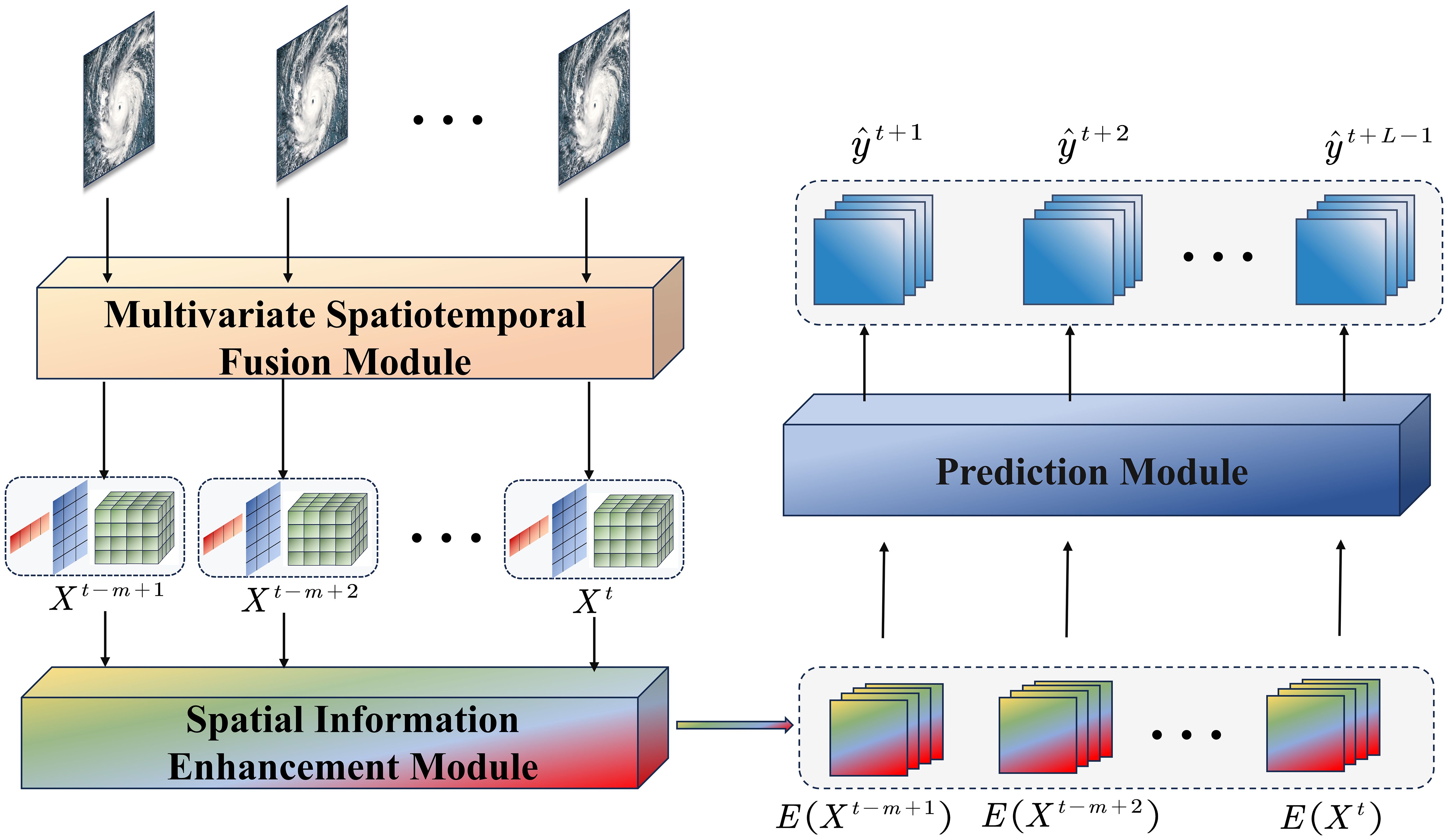
Figure 1. The framework of FS-STFNet.

3.1 Data fusion module

Accurate prediction of TC intensity relies on the effective fusion of multisource data. Since different datasets (e.g., satellite images, meteorological model outputs, etc.) often have varying spatial and temporal resolutions, standardizing the spatial scale of these data is key to improving prediction accuracy. To address this, a data fusion module includes spatial resolution standardization, cropping, and concatenation is designed to provide data foundation for TCs intensity forecasting.

In data fusion module, the region containing the TC core is first cropped into a square shape. The cropping is centered at the current eye region position p with a side distance r, which defines the focal area focusing on the TC core. Given the typical TC influence range of 600–1000 km, the parameter r is set to 5°based on the average TC scale. This cropping process eliminates irrelevant regions, reducing interference and improving the model’s ability to detect TCs intensity changes.

3.2 Spatial information enhancement module

Figure 2 depicts the framework of the Spatial Information Enhancement Module. In this study, the multisource environmental variable data can be modeled as a three-dimensional spatiotemporal environmental variable field, consisting of TCs temporal sequence data (real path information, TCs intensity, pressure, central wind speed, movement speed, and movement direction), atmospheric reanalysis data, and remote sensing data. These are represented as environmental variable observations $X^t=[X_p^t,X_a^t,X_{rs}^t]$. Specifically, $X_p^t$ represents the TCs temporal sequence data, $X_a^t$ represents the atmospheric reanalysis data, and $X_{rs}^t$ represents the remote sensing data.

Figure 2

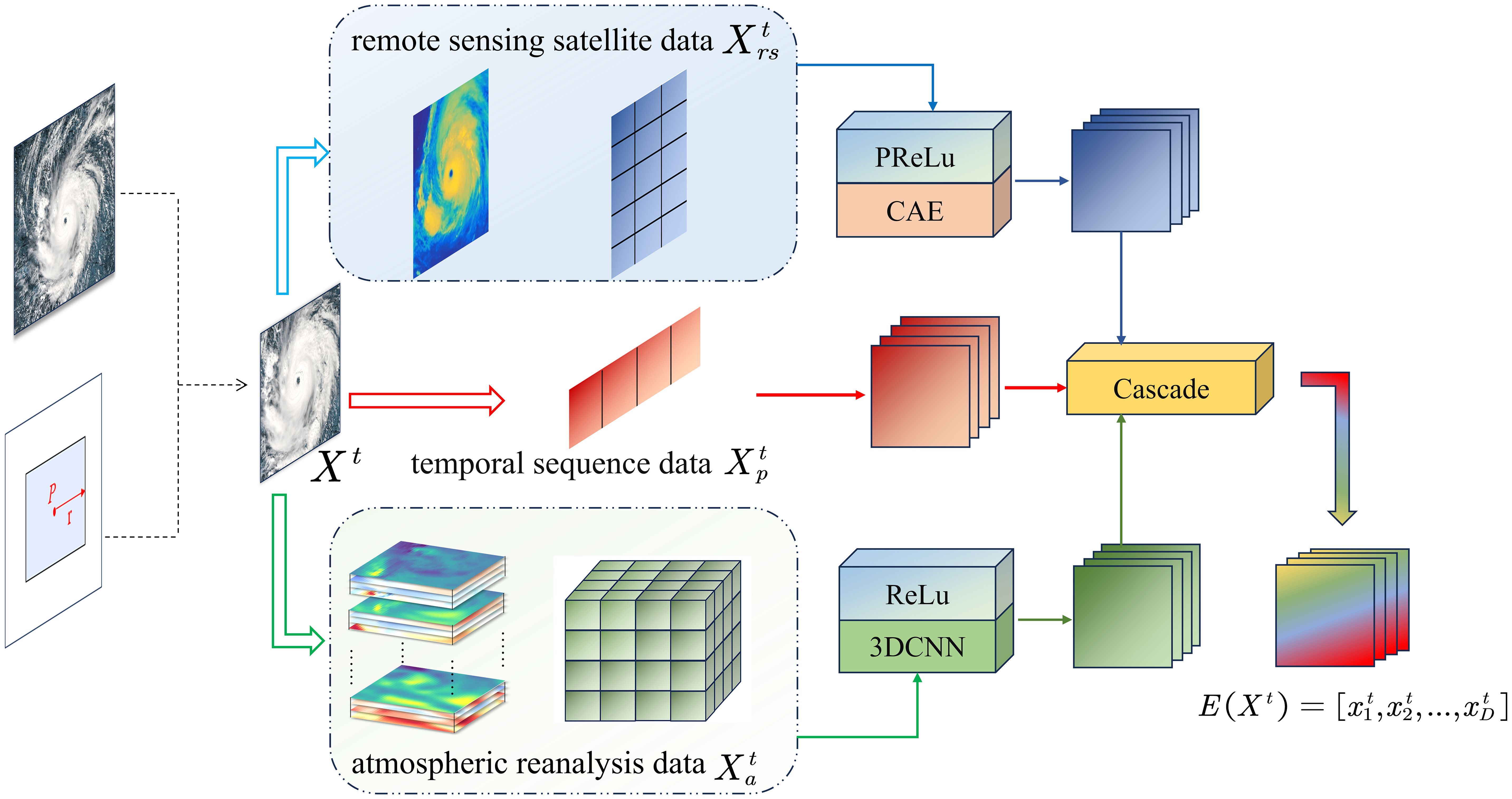
Figure 2. The framework of the spatial information enhancement module.

The spatial information enhancement module proposed in this study features two key improvements: On one hand, addressing the heterogeneity of multi-source data. It employs different convolutional neural networks to extract and enhance features from multi-source environmental data. Specifically, CAE is used to enhance spatial features from remote sensing data and 3DCNN is applied to capture spatiotemporal coupling features from atmospheric reanalysis data, in order to mine the core information of different data sources more accurately. On the other hand, it unifies the spatial scales of remote sensing data and atmospheric reanalysis data to ensure spatial consistency in fusion. Through a cascade operation, it deeply integrates features of different dimensions with TCs temporal sequence data, forming a high-dimensional spatial feature of the feature-enhanced multi-source environmental data $E(X^t)=[x_1^t,x_2^t,\dots ,x_D^t]$ that incorporates spatial details, spatiotemporal dynamics, and temporal sequence trends. Here, D denotes the number of variables of the high-dimensional spatial features of the data.

3.2.1 Remote sensing feature enhancement

Remote sensing data $X_{rs}^t$ typically contains rich spatial information, but this information may be noisy or suffer from inconsistent image quality due to changes in weather conditions. Therefore, feature enhancement techniques are employed to improve the quality of data by reinforcing the representation capacity of salient features, which is particularly crucial when data samples are limited. In this study, a CAE model is employed to enhance remote sensing features, thereby enabling more effective extraction of both global and local spatial features. Unlike ordinary autoencoders, CAE no longer uses fully-joined operations in encoding and decoding (Betechuoh et al., 2006), but instead use convolution and deconvolution operations. The working process of the CAE mainly includes encoding, decoding and parameter learning (Zhu et al., 2016).

The model used in this study is illustrated in Figure 3 and consists of an encoding module, a feature compression module, and a data expansion module. The encoder is composed of three convolutional layers and pooling layers, which progressively compress the spatial information of the image. The three-level convolutional layer structure is as follows:

Figure 3

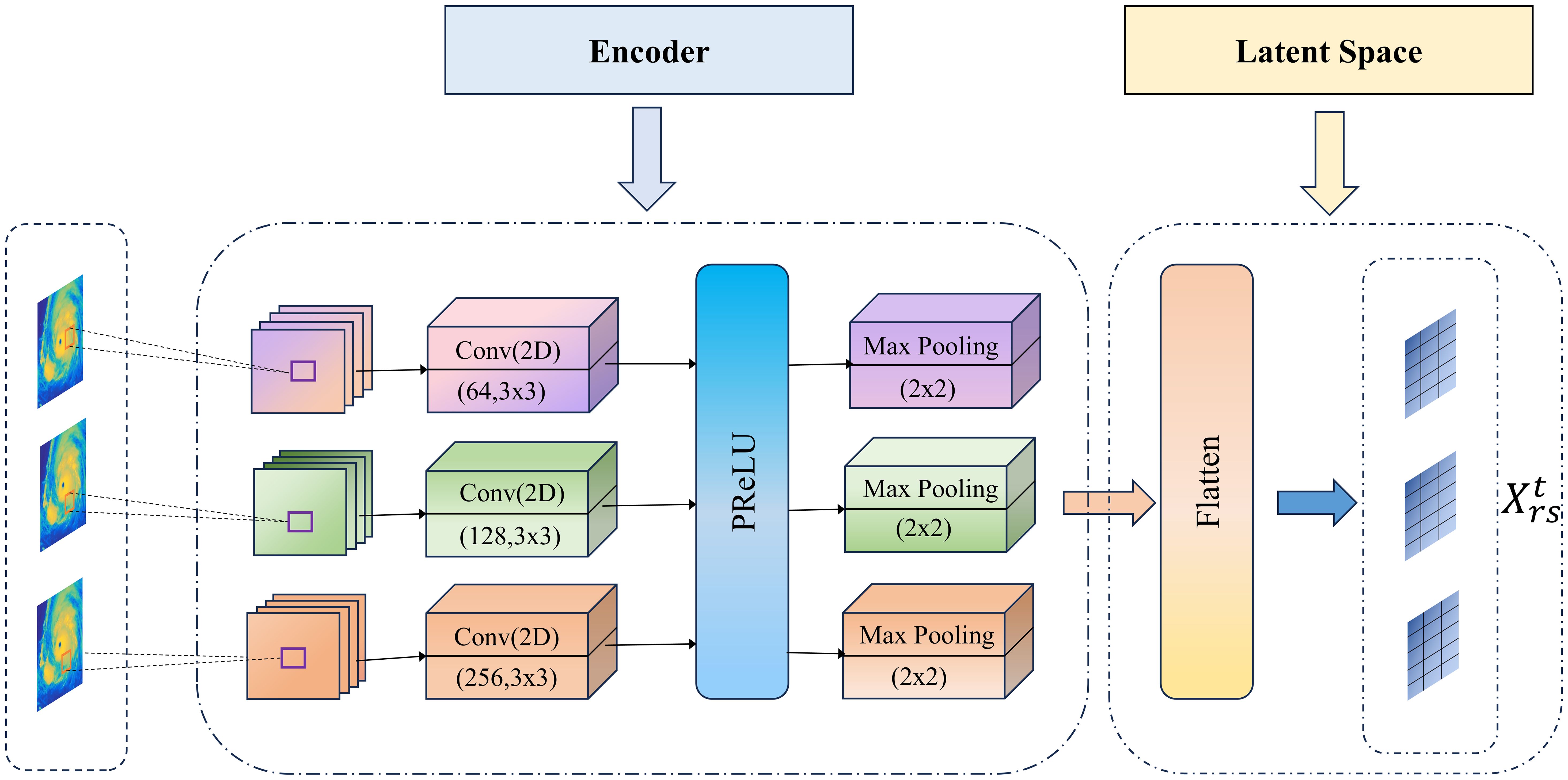
Figure 3. The structure of convolutional autoencoder.

The first layer employs 64 convolutional kernels, which increase to 128 in the second layer and further expand to 256 in the third layer. The kernel size of all convolutional layers are 3×3. After each convolutional operation, the PReLU activation function is applied to handle nonlinear transformations, which is mathematically expressed as Equation 1:

$\begin{array}{ll}{x}_{i+1}=PReLU(Conv2D(x_i)),& (1)\end{array}$

$x_i$ represents the input to the i-th layer, $Conv2D$ refers to the convolution operation, and $PReLU$ is the activation function.

Each convolutional level is followed by a 2×2 max pooling operation, progressively compressing the spatial dimensions, mathematically expressed as Equation 2:

$\begin{array}{ll}{x}_{last}=MaxPool(x_{i+1}),& (2)\end{array}$

After three convolution and pooling operations, the model compresses each time step of the remote sensing image into a 400-dimensional low-dimensional feature, representing the latent feature space of the data. The flattening process is, as Equation 3:

$\begin{array}{ll}{X}_{rs}^t=Flatten(x_{last}),& (3)\end{array}$

$X_{rs}^t$ is the output of the final convolutional pooling layer, and the flattening operation converts it into a one-dimensional vector.

The decoding process is to perform a deconvolution operation on the hidden layer data, so that the output data is restored to the dimension of the input data (Kundur and Hatzinakos, 1996). In this study, the decoder is not used for image reconstruction, however, its presence ensures the completeness of the autoencoder.

3.2.2 Meteorological feature enhancement

Atmospheric reanalysis data $X_a^t=[X_r^t,X_k^t,X_u^t,X_v^t]$ (i.e. relative humidity, temperature, horizontal wind components, and vertical wind components) play a crucial role in TC intensity prediction and other meteorological studies. Meteorological data typically exhibit significant spatiotemporal characteristics. Specifically, such data not only possess a spatial structure (e.g., the width and height of an image) but also demonstrate temporal dependencies across different time points. With the continuous increase in data volume, effectively processing and analyzing these high-dimensional datasets has become a major challenge. Traditional dimensionality reduction techniques, such as Principal Component Analysis (PCA), are often constrained by their linear assumptions when handling large-scale spatiotemporal data, making them inadequate for capturing complex nonlinear structures within the data. In this study, 3DCNN is employed to enhance meteorological feature extraction. As an extension of 2DCNN, the 3DCNN model introduces the temporal dimension as an additional input dimension (Wu et al., 2022). It performs convolutions across the spatial, temporal, and channel dimensions, enabling the effective capture of spatiotemporal patterns within the data.

The 3DCNN model structure used in this study is illustrated in Figure 4, with a core design that integrates spatiotemporal feature extraction and data compression mechanisms. The specific workflow is as follows:

Figure 4

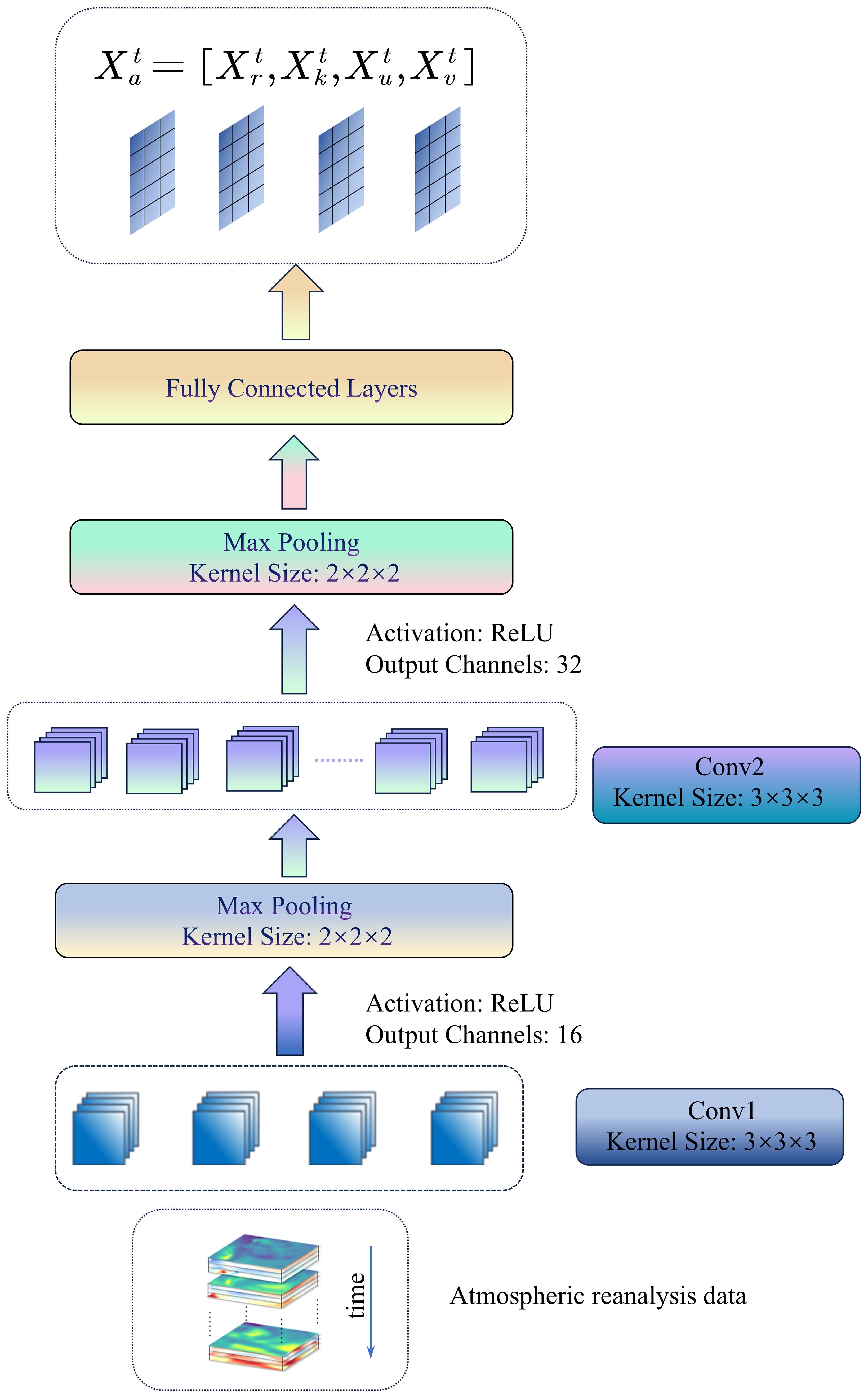
Figure 4. The structure of 3DCNN.

The model input consists of raw atmospheric reanalysis data, and its main architecture is composed of two levels of three-layer convolutional modules. The initial feature extraction (Conv1) utilizes 3×3×3 convolutional kernels, which slide along the temporal and spatial dimensions. The mathematical formulation is, as Equation 4:

$\begin{array}{ll}f(x,y,z)={\sum }_{i=-k}^k{\sum }_{j=-k}^k{\sum }_{l=-k}^{k}f(i,j,l)\times g(x-i,y-j,z-l),& (4)\end{array}$

Where $f(i,j,l)$ represents the convolutional kernel, and represents the input data. The output of this layer is a 16-channel feature map, which, after being enhanced by the ReLU activation function to improve nonlinear representation capability, undergoes 2×2×2 max pooling to reduce feature dimensions and eliminate redundant information. The deep feature compression stage (Conv2) continues to utilize 3×3×3 convolutional kernels to further extract high-order spatiotemporal correlation features, with the output channel dimension expanded to 32. Similarly, a 2×2×2 pooling operation is applied to further reduce parameter complexity and mitigate the risk of overfitting.

After two stages of convolution and pooling, the feature maps are flattened into a one-dimensional vector and fed into a fully connected layer for global information integration, ultimately generating an enhanced spatiotemporal feature. This design leverages a hierarchical and progressive feature abstraction mechanism, thus significantly improves the ability of the model to capture complex spatiotemporal patterns in atmospheric reanalysis data while maintaining a balance between computational efficiency and generalization capability.

The feature aggregation process for the three-dimensional environmental variable field observation data $X^t=[X_p^t,X_a^t,X_{rs}^t]$ can be expressed by Equation 5. Here, $f(*)$ represents the concatenation operation, $f_{cae}(*)$ represents the convolutional autoencoder operation, and $f_{3d}(*)$ represents the 3DCNN operation. Given a sequence of environmental variable observations $X=[X^{t-m+1},X^{t-m+2},\dots ,X^t]$, the feature aggregation module generates the global spatial feature representation sequence $E(X)=[E(X^{t-m+1}),E(X^{t-m+2}),\dots ,E(X^t)]$ for the input sequence.

$\begin{array}{ll}E(X^t)=f(X_p^t,f_{cae}(X_{rs}^t),f_{3d}(X_a^t)),& (5)\end{array}$

3.3 Prediction module

The framework of the prediction module is shown in Figure 5. The core component is the ARNN, whose storage structure is a multilayer feedforward neural network (Chen et al., 2020). For each TC, instead of taking $X^t$ as input, this architecture extracts high-dimensional spatial features from $E(X^t)=[x_1^t,x_2^t,\dots ,x_D^t]$ with t=1,2,…,n (i.e., the multi-source environmental data after feature enhancement in Section 3.2), and constructs a corresponding delay sequence $Y^t=[y^t,y^{t+1},\dots ,y^{t+L-1}]$. This delay sequence, for any target variable $y$ to be predicted (where $y^t=x_k^t$ represents the target variable, k=1,2,…,D), can be formed using a delay embedding strategy with an embedding dimension L>1. Here, we set the target variable $y^t$ as the maximum sustained wind speed near the center of the TC at time t. Thus, spatiotemporal transformation equation (STI) (Chen et al., 2020) is improved as the enhanced STI, which is expressed as Equation 6:

Figure 5

Figure 5. The framework of the prediction module.

$\begin{array}{ll}\{\begin{array}{c}\Phi [E(X^t)]=Y^t\\ Y^t=\Psi [E(X^t)]\end{array},& (6)\end{array}$

However, finding such nonlinear functions Φ and Ψ is often a challenging task. These can be linearized into the form of Equation 7:

$\begin{array}{ll}\{\begin{array}{c}A[E(X^t)]=Y^t\\ Y^t=B[E(X^t)]\end{array},& (7)\end{array}$

Where AB=I, A and B are matrices of size L × D and D× L, I is the identity matrix of size L× L.

The target vector $Y^t$ used for prediction is processed by a neural network F with two weight matrices, A and B. The architecture aims to simultaneously solve both the forward and conjugate forms of the enhanced STI equation to enhance robustness. Through processing by the neural network F, the enhanced STI equation is transformed into Equation 8:

$\begin{array}{ll}\{\begin{array}{c}AF[E(X^t)]=Y^t\\ Y^t=BF[E(X^t)]\end{array},& (8)\end{array}$

Thus, the information flow of the prediction framework can be represented by $F[E(X^t)]\to Y^t\to F[E(X^t)]$.

In this study, the neuron weights of the multi-layer feedforward neural network are randomly generated. The network consists of four layers, and each layer has 500 neurons, with the hyperbolic tangent function (tanh) used as the activation function. During the training process, the input data $E(X^t)$ is first normalized, and high-dimensional features are extracted through forward propagation.

During the forecasting process, the weight matrices A and B are initially given as null matrices first. Then, matrix B is updated through a dropout scheme. Subsequently, matrices A and $Y^t$ are updated based on B. Checking the convergence, updating matrix B in the next iteration if the convergence condition is not satisfied. After a sufficiently large number of such iterations, if the convergence condition is satisfied, then matrices A, B as well as the unknown part of $Y^t$ are determined and finally output the multi-step prediction values $\{{\widehat{y}}^{n+1}, {\widehat{y}}^{n+2},\dots , {\widehat{y}}^{n+L-1}\}$. The details of the calculation process can be found in the reference (Chen et al., 2020).

4 Results

4.1 Experiment settings

This study treats TC intensity prediction as a sequence-to-sequence prediction task, where the environmental variable observation data from the first 4 time steps are used as input, and the intensity data from the following 2 time steps are set as the prediction target. This can be simply represented as a 4→2 prediction. Therefore, m is set to 4, and L is set to 3 in the model. Additionally, best track data, remote sensing data, and atmospheric reanalysis data are set as different input parameters to evaluate their impact on the prediction model.

In this study, quantitative evaluation metrics are used to assess the performance of the prediction model, primarily focusing on the Mean Absolute Error (MAE), which is defined as follows in Equation 9, where $y_i$ represents the actual value, ${\widehat{y}}_i$ represents the predicted value, and N is the total number of data samples to be evaluated.

$\begin{array}{ll}MAE=\frac{1}{N}{\sum }_{i=1}^N|y_i-{\widehat{y}}_i|,& (9)\end{array}$

4.2 TC intensity short-term prediction results

To verify the effectiveness of FS-STFNet in TC intensity prediction, this study selects the GRU and Long Short-Term Memory (LSTM) networks as benchmarks for classic time series forecasting models. Due to their powerful ability to model temporal dependencies, GRU and LSTM have become widely used deep learning architectures in fields such as finance (Dip-Das et al., 2024; Liu and Lai, 2025) and environmental science (Raychaudhuri and Babu, 2022). Since both methods require a large number of samples for training, we use TCs data from 2008 to 2018 for training, the test data period is 2019-2021, which is consistent with the test data used of our method. The experimental results are shown in Table 1.

Table 1

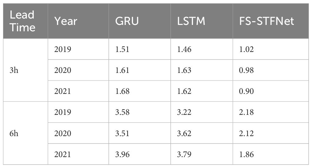
Table 1. Comparison of MAE results of different methods.

Experimental results demonstrate that FS-STFNet exhibits significant advantages in short-term prediction of TC intensity. At 3-hour lead prediction, FS-STFNet reduces the MAE by 40%–47% and 31%–45% compared to GRU and LSTM, respectively. As for 6-hour lead, FS-STFNet also remains the supeority. The results demonstrate that through multi-source data fusion and enhancement, FS-STFNet is able to capture the high-frequency nonlinear variations in TC intensity.

Figure 6 visualizes the spatial distribution of TC trajectories and intensity prediction errors in the Northwest Pacific from 2019 to 2021. The heatmap illustrates the MAE result at each nodal point along the cyclone paths, with the top-to-bottom arrangement corresponding to the years 2019–2021. The left panels represent the 3-hour prediction results, while the right panels display the 6-hour prediction results. The color gradient from blue to red indicates error values ranging from 0 to 4, where warmer colors signify higher errors. The FS-STFNet model demonstrates a strong capability in short-term TC intensity prediction. Across all three years, the 3-hour prediction error remains at a low level.

Figure 6

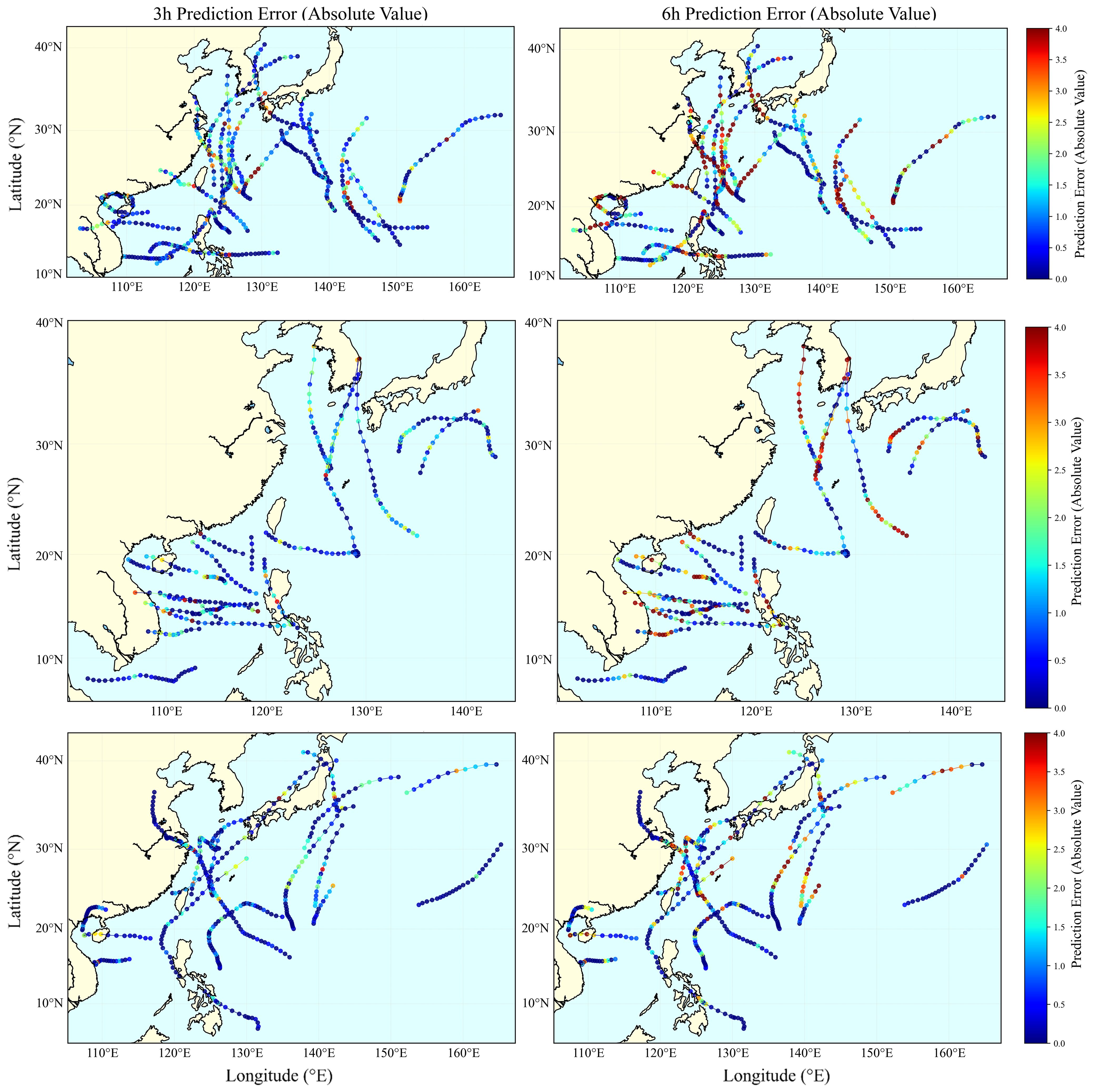
Figure 6. TC intensity prediction error of FS-STFNet from 2019 to 2021.

As we can see from Figure 6, the prediction results of 2021 and 2020 is better than 2019. We attempt to figure out the reason and find that multiple TCs simultaneous presence in 2019, resulting in exceptional complexity of environment. For example, “Lekima”, “Krosa”, and “Bailu” were nearly concurrently active. Although the centers of these TCs were separated, their indirect interactions significantly altered the regional atmospheric circulation patterns. In addition, TCs “Fung-wong”, “Kalmaegi” and “Fengshen” also exhibit this phenomenon. Compared to 2019, TCs during 2020–2021 are more dispersed, with individual cyclones generally exhibiting relatively stable trajectories and structural characteristics. Consequently, FS-STFNet is able to better capture the intensity evolution of these systems, ultimately leading to more accurate predictions.

From the spatial perspective, the spatial heterogeneity of TC intensity prediction errors from 2019 to 2021 was primarily driven by the combined effects of geographical environments and TC-system interactions. Studies have shown that terrestrial friction alters the radial inflow structure and vertical motion distribution within the boundary layer, thereby accelerating energy dissipation in the TC core region (Zhao et al., 2015). Specifically, when a TC approaches or makes landfall, the abrupt transition in surface characteristics from ocean to land disrupts energy supply and enhances frictional dissipation, thereby increasing forecast errors. For example, after “Lekima” made landfall in Shandong in 2019, its 6-hour prediction error was significantly higher than its 3-hour prediction error. Similarly, “Higos” in 2020, after landfall in Guangdong, was affected by land friction and environmental field variations, leading to an underestimation of its rapid intensity decay. In 2021, “In-Fa” slowed down after making landfall in Zhejiang, further complicating its intensity evolution and increasing forecast errors. Additionally, the eastern coastal region of China has a complex geographical structure—including irregular coastlines (e.g., the Zhoushan Archipelago), multi-tiered coastal mountain ranges (e.g., those in Fujian and Zhejiang), and dense urban clusters—that significantly influence the spatial distribution of forecast errors (Liu, 2013). When TC circulation interacts with mountainous terrain, windward slope effects can enhance low-level horizontal convergence, leading to reduced convective system organization (Tan and Wu, 2000). For example, when “Bailu” was active along the coastal region of Fujian in 2019, its circulation was influenced by the coastal mountain ranges, leading to deviations in rainfall distribution and affecting the accuracy of intensity forecasts. Furthermore, in 2021, “Lupit” experienced asymmetric eyewall collapse while traversing the Taiwan Strait due to complex terrain influences, significantly increasing intensity prediction errors.

The prediction errors in TCs from 2019 to 2021, beyond spatiotemporal factors, were closely associated with the weak intensity characteristics and abrupt structural transformations of certain TCs. Weak TCs, due to their limited energy reserves, are more susceptible to subtle environmental perturbations. For instance, “Wipha” exhibited multiple “serpentine oscillations” in its trajectory while active over the South China Sea, as it was alternately dominated by the southwestern monsoon and the peripheral flow of the subtropical high, leading to significant prediction errors at certain nodes. Furthermore, the sudden dissipation of the TC eye, as observed in “Sinlaku” when approaching Hainan Island, triggered a reorganization of the circulation, resulting in intensity prediction deviations. These cases indicate that weak intensity and structural instability amplify environmental perturbations and destabilize the self-organization capacity of the system, which markedly elevates the challenge of capturing nonlinear evolutionary patterns in predictive models.

4.3 The impact of different input parameters

This section explores the impact of different input parameters on TC intensity prediction. Figure 7 visualizes the MAE results of different TCs in 2019-2021. The input data types include time series data (i.e. TC best track data), time series data combined with remote sensing data, and aggregated data that integrates time series data, remote sensing data, and meteorological data.

Figure 7

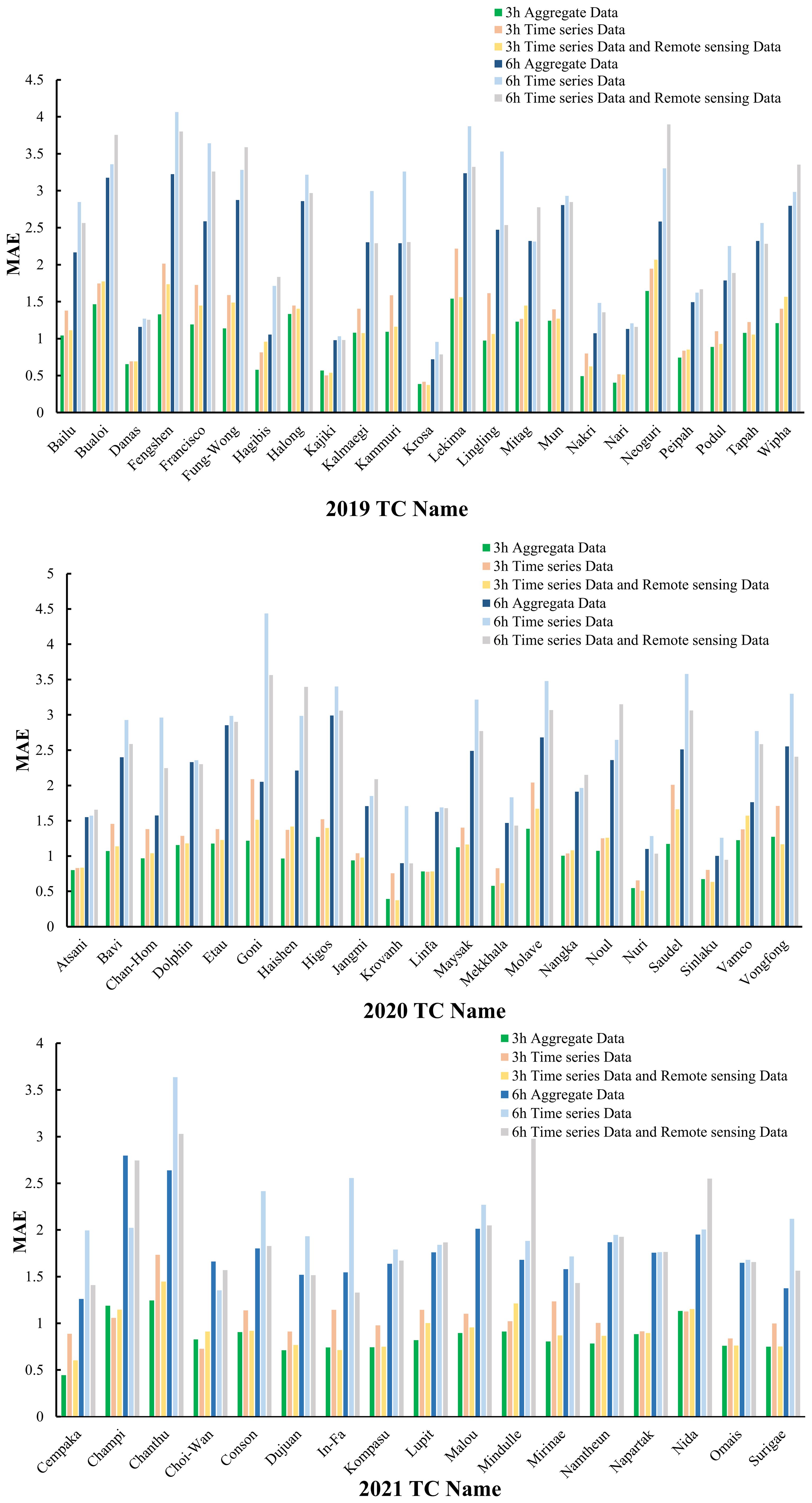
Figure 7. MAE results of different TCs in 2019-2021.

In most TCs from 2019 to 2021, as the forecast lead time increased from 3 to 6 hours, the prediction errors of all three data types rose, with time series data showing the largest errors and aggregate data the smallest. Taking “Chan-Hom” and “Goni” as examples, the 6-hour lead MAE results of using time series data are 2.96, 4.43, respectively, which increased about 54% compared to 3-hour lead. As for using aggregate data, the error increased from 3-hour lead to 6-hour lead is much smaller compared to using time series data, only 39% increased.

These examples illustrate the importance of meteorological and remote sensing data for TC intensity prediction and the superiority of aggregate data in continuous forecasting.

As for some TCs like “Danas”, “Linfa” and etc., the MAE results of using time series data may be close to aggregate data. This is because that these TCs are very stable during the development stages. For example, “Linfa” and “Choi-Wan” remained mostly at the tropical storm stage with wind speeds of 17.2-24.4m/s or the tropical depression stage with wind speeds of 10.8-17.1m/s during their longer life cycles, using time series data could also effectively reflect their intensity trends.

With different input parameters, the overall results show that using single time series data have largest prediction errors, while combining remote sensing data can reduce the errors. Aggregate data, integrating multi-source information, further improve the prediction accuracy in most TCs. However, as the lead time increases, the atmospheric environment becomes more complex, amplifying the impact of multiple sources of error and increasing prediction errors and uncertainties for three types of input parameters.

4.4 Comparison with different feature enhancement methods

To validate the superiority of the feature extraction methods for remote sensing and meteorological features used in the spatial information enhancement module, this section employs 2DCNN and CAE for feature extraction of remote sensing data, and 3DCNN and ConvAutoencoder (CA) for meteorological data feature extraction. As a baseline, the RAW-RAW column shows the results without applying any feature enhancement techniques. These results exhibit generally higher prediction errors, especially as the lead time increases, indicating the limitations of models without spatial information enhancement module. Comparison results of different feature enhancement methods are shown in Figure 8. A comprehensive comparison based on different forecast lead times shows that after using 2DCNN-CA and CAE-CA for feature extraction, the prediction errors are relatively small, but still not as good as the feature extraction methods used in this study. The 2DCNN-3DCNN methods result in larger prediction errors. Moreover, as the forecast lead time increases from 3 hours to 6 hours, the impact of different enhancement methods on TC intensity prediction becomes more significant. At the 3-hour forecast lead time, the errors from different enhancement models are generally small, especially with the 2DCNN-CA and CAE-CA methods, where the error values are relatively low. However, when the forecast lead time extends to 6 hours, the prediction errors increase significantly.

Figure 8

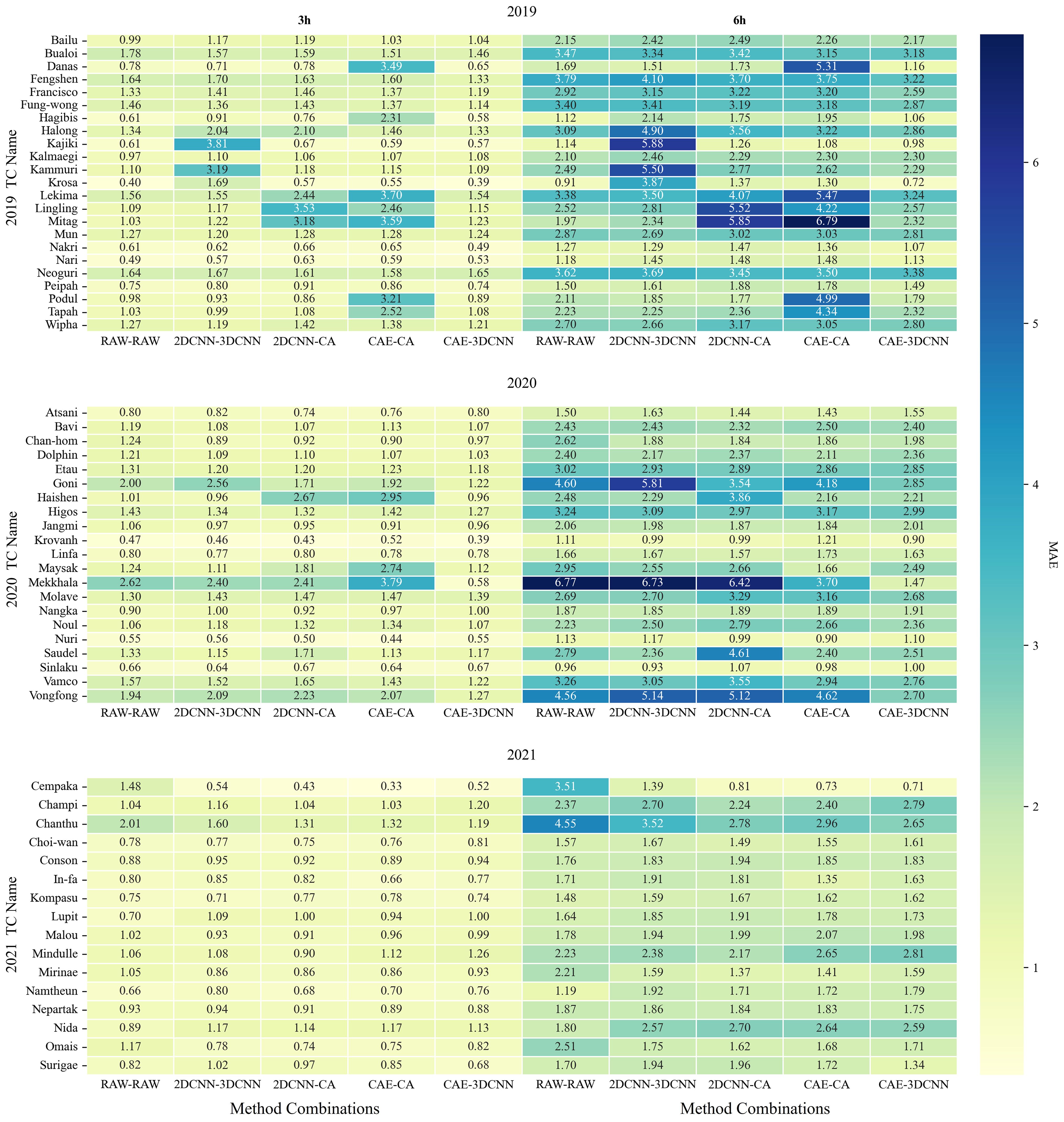
Figure 8. Comparison results of different feature enhancement methods.

5 Discussion

This paper proposes a spatiotemporal deep network-based method for TC intensity prediction, aiming to address the limitations of traditional numerical forecasting and data-driven models in terms of predictive accuracy and applicability. The proposed approach integrates a multidimensional spatiotemporal information fusion module, a spatial feature enhancement module, and a prediction module to construct an efficient representation framework for multi-source meteorological data, incorporating TC time-series data, atmospheric reanalysis data, and remote sensing satellite data. The core advantages of this method include:

The adoption of spatiotemporal feature enhancement techniques, where a CAE and a 3DCNN are employed to extract spatial features from remote sensing data and capture the spatiotemporal coupled features of meteorological data, effectively reducing noise and lowering data dimensionality;

The introduction of an ARNN as the prediction module, leveraging a dynamic weight adjustment mechanism to capture the nonlinear evolution patterns of TC intensity, thereby significantly improving the robustness of short-term prediction;

The capability to support independent modeling for individual TCs, ensuring high predictive performance even in scenarios with limited historical data.

The experiment focuses on TCs in the Northwest Pacific from 2019 to 2021, integrating JTWC best track data, Copernicus atmospheric reanalysis data, and Himawari-8 satellite infrared remote sensing data to construct a multi-source dataset. The results indicate that for short-term prediction of TC intensity, our model outperforms GRU and LSTM models. Furthermore, the multi-source data fusion strategy enables optimal prediction accuracy when the TC structure is clear and the path is stable. For weak intensity TCs or cases affected by land friction or abrupt sea surface temperature changes, the model can further reduce prediction bias through targeted adjustments.

This method provides a promising technical approach for short-term TC intensity forecasting. Its modular design can be extended to the prediction of other extreme weather events, offering significant value for disaster prevention and mitigation applications. Future work will focus on integrating physical mechanism constraints to improve the generalization capacity of models for abnormal TC systems.

6 Conclusion

A spatiotemporal deep learning method FS-STFNet is proposed for short-term prediction of TC intensity. FS-STFNet model consists of the Multivariate Spatiotemporal Fusion Module, the Spatial Information Enhancement Module, and the Prediction Module. The spatial features of historical multisource data including remote sensing images and atmospheric reanalysis data are adaptively captured and enhanced through the Spatial Information Enhancement Module. Furthermore, the ARNN model is applied in the Prediction Module to predict TC intensity accurately from small-sample data. The experimental results demonstrate that our model outperforms other methods in 3 and 6-hour lead forecasting. The proposed FS-STFNet is applicable to short-term TC intensity forecasting, especially showing superiority in forecasting tropical cyclones with stable structures and enabling robust predictions for individual TCs with limited historical records. Future research will attempt to consider more factors and integrating physical mechanism constraints for long-term TC intensity forecasting.

Data availability statement

The original contributions presented in the study are included in the article/supplementary material. Further inquiries can be directed to the corresponding author.

Author contributions

MQ: Conceptualization, Funding acquisition, Methodology, Resources, Software, Writing – original draft, Writing – review & editing. JW: Data curation, Software, Validation, Visualization, Writing – original draft, Writing – review & editing. YW: Software, Validation, Visualization, Writing – original draft, Writing – review & editing. YZ: Software, Validation, Writing – review & editing. WL: Data curation, Visualization, Writing – review & editing. SS: Conceptualization, Funding acquisition, Writing – review & editing.

Funding

The author(s) declare financial support was received for the research and/or publication of this article. This research was funded by the National Natural Science Foundation of China (U2442203, 42306213) and Provincial Undergraduate Training Program on Innovation and Entrepreneurship (S202410497252).

Conflict of interest

The authors declare that the research was conducted in the absence of any commercial or financial relationships that could be construed as a potential conflict of interest.

Generative AI statement

The author(s) declare that no Generative AI was used in the creation of this manuscript.

Any alternative text (alt text) provided alongside figures in this article has been generated by Frontiers with the support of artificial intelligence and reasonable efforts have been made to ensure accuracy, including review by the authors wherever possible. If you identify any issues, please contact us.

Publisher’s note

All claims expressed in this article are solely those of the authors and do not necessarily represent those of their affiliated organizations, or those of the publisher, the editors and the reviewers. Any product that may be evaluated in this article, or claim that may be made by its manufacturer, is not guaranteed or endorsed by the publisher.

References

Alpers W. R. and Bruening C. (1986). On the relative importance of motion-related contributions to the SAR imaging mechanism of ocean surface waves. IEEE Trans. Geosci. Remote Sens. GE-24, 873–885. doi: 10.1109/TGRS.1986.289702

Crossref Full Text | Google Scholar

Bauer P., Thorpe A., and Brunet G. (2015). The quiet revolution of numerical weather prediction. Nature 525, 47–55. doi: 10.1038/nature14956

PubMed Abstract | Crossref Full Text | Google Scholar

Betechuoh L., Marwala T., and Tettey T. (2006). Autoencoder networks for HIV classification Brain. Curr. Sci. 91 (11), 1467–1473. Available online at: http://www.jstor.org/stable/24093843.

Google Scholar

Chen P., Liu R., Aihara K., and Chen L. N. (2020). Autoreservoir computing for multistep ahead. Prediction based on the spatiotemporal information transformation. Nat. Commun. 11, 4568. doi: 10.1038/s41467-020-18381-0

PubMed Abstract | Crossref Full Text | Google Scholar

Dip-Das J., Thulasiram R. K., Henry C., and Thavaneswaran A. (2024). Encoder–decoder based LSTM and GRU architectures for stocks and cryptocurrency prediction. J. Risk Financial Manage. 17, 200. doi: 10.3390/jrfm17050200

Crossref Full Text | Google Scholar

Dong P. P., Lian J., Yu H., Pan J. G., Zhang Y. P., and Chen G. M. (2022). Tropical cyclone track prediction with an encoding-to-forecasting deep learning model. Weather Forecasting 37, 971–987. doi: 10.1175/WAF-D-21-0116.1

Crossref Full Text | Google Scholar

Huang C., Bai C., Chan S. X., and Zhang J. L. (2022). MMSTN: A multi-modal spatial-temporal network for tropical cyclone short-term prediction. Geophysical Res. Lett. 49 (4), e2021GL096898. doi: 10.1029/2021gl096898

Crossref Full Text | Google Scholar

Huang X. Y., Jin L., and Shi X. M. (2011). “A Nonlinear Artificial Intelligence Ensemble Prediction Model Based on EOF for Typhoon Track,” in Proceedings of the 2011 Fourth International Joint Conference on Computational Sciences and Optimization (Kunming and Lijiang City, China: IEEE), 1329–1333 doi: 10.1109/CSO.2011.48

Crossref Full Text | Google Scholar

Huang C., Mu P., Zhang J. L., Chan S. X., Zhang S. Q., Yan H. T., et al. (2025). Benchmark dataset and deep learning method for global tropical cyclone forecasting. Nat. Commun. 16, 5923. doi: 10.1038/s41467-025-61087-4

PubMed Abstract | Crossref Full Text | Google Scholar

Kim D. and Matyas C. J. (2024). Classification of tropical cyclone rain patterns using convolutional autoencoder. Sci. Rep. 14, 791. doi: 10.1038/s41598-023-50994-5

PubMed Abstract | Crossref Full Text | Google Scholar

Kundur D. and Hatzinakos D. (1996). Blind image deconvolution revisited. IEEE Signal Process. Magazine 13, 61–63. doi: 10.1109/79.543976

Crossref Full Text | Google Scholar

LeCun Y., Bengio Y., and Hinton G. (2015). Deep learning. Nature 521, 436–444. doi: 10.1038/nature14539

PubMed Abstract | Crossref Full Text | Google Scholar

Lee J., Im J., and Shin Y. (2024). Enhancing tropical cyclone intensity forecasting with explainable deep learning integrating satellite observations and numerical model outputs. iScience 27, 109905. doi: 10.1016/j.isci.2024.109905

PubMed Abstract | Crossref Full Text | Google Scholar

Liu J. Y. (2013). Status of marine biodiversity of the China seas. PLoS One 8, e50719. doi: 10.1371/journal.pone.0050719

PubMed Abstract | Crossref Full Text | Google Scholar

Liu B. C. and Lai M. Z. (2025). Advanced machine learning for financial markets: A PCA-GRU-LSTM approach. J. Knowl. Econ. 16, 3140–3174 doi: 10.1007/s13132-024-02108-3

Crossref Full Text | Google Scholar

Lu J. Q., Wang Z. D., Cao J. D., Ho D. W. C., and Kurths J. (2012). Pinning impulsive stabilization of nonlinear dynamical networks with time-varying delay. Int. J. Bifurcation Chaos 22, 1250176. doi: 10.1142/s0218127412501763

Crossref Full Text | Google Scholar

Milojkovic J. and Litovski V. (2011). Short-term forecasting in electronics. Int. J. Electron. 98, 161–172. doi: 10.1080/00207217.2010.482025

Crossref Full Text | Google Scholar

Raychaudhuri S. J. and Babu C. N. (2022). On the domain aided performance boosting technique for deep predictive networks: A COVID-19 scenario. Inf. Technol. Disasters 16, 111–125. doi: 10.3233/IDT-200167

Crossref Full Text | Google Scholar

Tan Z. M. and Wu R. S. (2000). A theoretical study of low-level frontal structure in the boundary layer over orography: part I: cold front and uniform geostrophic flow. Acta Meteorologica Sin. 58 (2), 137–150. doi: 10.11676/qxxb2000.015

Crossref Full Text | Google Scholar

Tong B., Wang X., Fu J. Y., Chan P. W., and He Y. C. (2022). Short-term prediction of the intensity and track of tropical cyclone via convLSTM model. J. Wind Eng. Ind. Aerodynamics 226, 105026. doi: 10.1016/j.jweia.2022.105026

Crossref Full Text | Google Scholar

Wang P. P., Wang P., Wang C., Xue B., and Wang D. (2022). Using a 3D convolutional neural network and gated recurrent unit for tropical cyclone track forecasting. Atmospheric Res. 269, 106053. doi: 10.1016/j.atmosres.2022.106053

Crossref Full Text | Google Scholar

Wu H. B., Ma X., and Li Y. B. (2022). Spatiotemporal multimodal learning with 3D CNNs for video action recognition. IEEE Trans. Circuits Syst. Video Technol. 32, 1250–1261. doi: 10.1109/TCSVT.2021.3077512

Crossref Full Text | Google Scholar

Xing L. W., Hu D. Y., and Tang L. L. (2011). “Development of Typhoon disaster risk evaluation and early warning system integrating real-time rainfall data from the satellite,” in Proceedings of the 19th International Conference on Geoinformatics (Shanghai, China: IEEE), 1–5. doi: 10.1109/GeoInformatics.2011.5981067

Crossref Full Text | Google Scholar

Xu G. N., Lin K. H., Li X., and Ye Y. M. (2022). SAF-net: A spatio-temporal deep learning method for typhoon intensity prediction. Pattern Recognit. Lett. 155, 121–127. doi: 10.1016/j.patrec.2021.11.012

Crossref Full Text | Google Scholar

Xu Z., Zou L., Lu X. Z., and Aizhu M. (2013). Fast prediction of typhoon tracks based on A similarity method and gis. Disaster Adv. 6 (6), 45–51.

Google Scholar

Zhang Z., Yang X. Y., Shi L. F., Wang B. B., Du Z. H., Zhang F., et al. (2022). A neural network framework for fine-grained tropical cyclone intensity prediction. Knowledge-Based Syst. 241, 108195. doi: 10.1016/j.knosys.2022.108195

Crossref Full Text | Google Scholar

Zhao X. T., Zhao Y. C., Cui C. G., Wang X. K., and Ke D. (2015). Analysis on track and intensity changes of STC Utor before and after its landing. Torrential Rain Disasters 34 (3), 197–205. Available online at: http://byzh.org.cn/en/article/id/2284.

Google Scholar

Zhu Z. T., Wang X. G., Bai S., Yao C., and Bai X. (2016). Deep learning representation using autoencoder for 3D shape retrieval. Neurocomputing 204, 41–50. doi: 10.1016/j.neucom.2015.08.127

Crossref Full Text | Google Scholar