Abstract
Amphipods play an important role in Southern Ocean trophic chains. Considering the key role of Pacific Ocean and sea ice ecosystems in the Earth system and the growing impact of global environmental change, it is important to collect information on the status of marine amphipod biodiversity. A total of 410 zooplankton samples were collected by BIONESS (Bedford Institute of Oceanography Net Environmental Sampling System) from 27 stations during the Vth ItaliaAntartide Expedition, between 25 November 1989 and 12 January 1990, in the Pacific sector of the Southern Ocean, from New Zealand to the Western Ross Sea. The aim of this study was to describe the composition, relative abundance, spatial distribution and latitudinal boundaries of pelagic amphipods. An additional goal was to describe the main water masses and the pack ice extent and its temporal evolution during the cruise and relate species assemblages to the physical structure of the region. A total of 2058 specimens of pelagic amphipods was counted, and 43 taxa belonging to 18 families were identified. Hyperiella dilatata was the most abundant species (45% of relative abundance) followed by Primno macropa (12%), Pseudorchomene plebs (12%) and Hyperiella macronyx (8%). The composition of amphipod species differed significantly between stations. Three different clusters were identified through the k-means algorithm based on species abundance and confirmed by an NMDS plot. Cluster 1 was mainly composed of the southernmost stations, Cluster 2 included the northernmost stations, while the stations in the central part were grouped in Cluster 3. A correlation between species composition and the sampled layers at the different stations was highlighted. Knowledge of amphipod biodiversity by means of this study can represent a baseline for future studies, to provide evidence of potential changes as signal of alterations in the environment.
1 Introduction
Amphipods occupy many different habitats in both the pelagic and benthic realms (De Broyer et al., 2007; De Broyer and Danis, 2011; De Broyer and Jażdżewska, 2014; Jażdżewska and Siciński, 2017). They also span the spectrum of trophic behaviors, from herbivory, carnivory and omnivory through to scavenging (Dauby et al., 2001a, b). Amphipod crustaceans exist across marine habitats from the polar regions to the tropics, providing a critical biological link between benthic/pelagic processes and marine/atmospheric ecosystems (Ritter and Bourne, 2024). Amphipods play important roles in Southern Ocean ecosystems, acting as a food source for both invertebrates (mainly polychaetes, echinoderms and squid), and higher trophic levels such as fish, seabirds and marine mammals (Duarte and Moreno, 1981; Jażdżewski, 1981; Jażdżewski and Konopacka, 1999; Dauby et al., 2003). According to the World Amphipoda Database (Horton et al., 2023), the order Amphipoda is divided into six marine accepted suborders: Amphilochidea, Colomastigidea, Hyperiidea, Hyperiopsidea, Pseudingolfiellidea and Senticaudata. Among these, the suborder Senticaudata is the most represented, followed by Amphilochidea and Hyperiidea.
Pelagic amphipods encompass only few species from the suborders Amphilochidea and Senticaudata, and instead many species from Hyperiidea (Sanvicente-Añorve et al., 2023). All these species are found worldwide (Sanvicente-Añorve et al., 2023). Amphipods of the suborder Amphilochidea inhabit both benthic and pelagic marine habitats, and were found in various environments, such as sands and muds, coral reefs and open oceans, playing important ecological roles as detritivores and predators. Autochthonous sympagic amphipods (i.e., those produced within the sea ice) have only been recorded from the Arctic (Hop et al., 2021), feeding on ice algae and pelagic fauna as well as detritus (Werner, 1997; Poltermann, 2001), while allochthonous sympagic organisms (i.e., those arising from outside of the sea ice habitat sensu stricto) have been recorded from both the Antarctic and the Arctic (Gullisen and Lonne, 1991). Seasonally, ice covers large areas, mainly over deep water, and pelago-sympagic organisms play a key role in utilizing the primary production from sea ice algae; e.g., it has been shown that the amphilochidean sympagic amphipod Eusirus laticarpus consumed from 54% - 67% of ice algal carbon (Kohlbach et al., 2018). In recent decades, a decrease in the abundance of these crustaceans has been detected in the Arctic (Hop et al., 2021), while in the Antarctic, research on diversity and abundance is still in its infancy. Therefore, despite important steps being taken in marine amphipod research, the roles of sympagic assemblages in polar marine ecosystems remain largely unknown (Arndt and Swadling, 2006). To understand how sea ice ecosystems will be influenced by climate change, obtaining baseline knowledge on the biodiversity of species is critical (IPCC, 2021).Differently from Amphilochidea, the suborder Hyperiidea is a primarily pelagic marine group, distributed from the upper ocean surface to the abyssopelagic depths. Their habitat is therefore, meso- and macrozooplankton biota, where many species live as parasites or predators of other gelatinous organisms such as salps and jellyfish, while other species are more free-living predators of small mesozooplanktonic animals, like copepods. Of these suborders, Hyperiidea is the most abundant, with 282 species described in the world (Horton et al., 2023). They exhibit high diversity in the oceanic zone (Bowman and Gruner, 1973; Lorz and Peracy, 1975; Violante-Huerta, 2019), while in neritic zones their diversity is lower, but abundance is higher (Gasca, 2004; Velázquez-Ramírez, 2021). Vertically in the ocean, order Amphipoda occur from surface to abyssal depths, as far down as the hadal zone (Vinogradov et al., 1996; Vinogradov, 1999). Hyperiideans are mainly carnivores and feed on other zooplankton organisms, such as Polychaeta, Chaetognatha, Copepoda, small crustaceans and other amphipods (Bowman, 1978; Williams and Robins, 1981; Zeidler, 1984; Sanvicente-Añorve et al., 2023). As hyperiid amphipods are known to occur in the vicinity of krill swarms (Pakhomov and Perissinotto, 1996; Dauby et al., 2003), they are likely to also contribute to the diets of plankton-feeding cetaceans.
It is well known that sea-ice variability affects biological processes and polar food webs (Massom and Stammerjohn, 2010; Castellani et al., 2020; Granata et al., 2022; Fraser et al., 2023; Swadling et al., 2023). The Southern Ocean is characterized by latitudinal variations in sea-ice concentration and extent at both local and regional scales (Ferola et al., 2023; Fraser et al., 2023). Recent observations in the Atlantic and Pacific sectors show a strong decrease in sea ice extent during the last four decades (Parkinson and Cavalieri, 2012; Stammerjohn et al., 2012; Yang et al., 2021; Wachter et al., 2021; Fraser et al., 2023), whereas in the Ross Sea a slight increase has been detected (Ferola et al., 2023). We now know that many key species, particularly copepods and amphipods, are abundant in the sea ice zone at both poles, either living within the brine channel system of the ice-crystal matrix or inhabiting the ice-water interface (Arndt and Swadling, 2006).
Considering the key role of the Pacific Ocean in the Earth system and the growing impact of global environmental change, it is important to collect information on the status of marine amphipod biodiversity as integral members of global ocean ecosystems (Ritter and Bourne, 2024). Amphipod families are common in the region under study; namely, the Pacific sector of the Southern Ocean, the Ross Sea and Terra Nova Bay. The suborders Amphilochoidea and Senticaudata are found on or near the seafloor, Hyperiidea and bentho-pelagic Amphilochoidea and Senticaudata are present in the water column, while the sea ice is habitat for epontic species (De Broyer and Jażdżewska, 2014; Minutoli et al., 2023). While there are several studies on Antarctic benthic amphipods, many areas of the continental shelf and the deep sea remain unexplored (Zeidler and De Broyer, 2009; De Broyer and Jażdżewska, 2014; Jażdżewska and Siciński, 2017; Minutoli et al., 2023). Notably, few studies have been carried out on pelagic species, and little is known about their vertical distribution or their biogeographical boundaries (Zeidler and De Broyer, 2009; Minutoli et al., 2023).
The amphipods analyzed in the present study were collected in oceanic waters characterized as permanently open ocean (POOZ), seasonal pack-ice (SIZ), or the pack ice zone (PIZ). The aim of this paper was to describe the composition, relative abundance, spatial distribution and latitudinal boundaries of pelagic amphipod species in the Pacific sector of the Southern Ocean, in the Ross Sea and within Terra Nova Bay, based on thinly stratified vertical sampling. An additional goal was to describe the main water masses and the pack ice extent and its temporal evolution during the cruise and relate species assemblages to the physical structure of the region.
2 Materials and methods
2.1 Sea ice conditions and sampling strategy
The Southern Ross Sea is characterized by the presence of a polynya, large area of open water surrounded by sea ice, that is generated by strong katabatic winds (a downslope wind caused by the flow of an elevated, high-density air mass into a lower-density air mass below under the force of gravity), that transport and control the dynamics and temporal coverage of sea ice (Zwally et al., 1983; Jacobs and Comiso, 1989). This physical phenomenon plays a major role in driving variability in the functioning of the ecosystem on a short time scale (Hecq et al., 1993). Typically, during late winter and early spring in the western Ross Sea, the ice-free surface spreads from south to north starting from the Ross Ice Shelf Polynya (RISP), causing the ice to retreat and melt and expose the water column to sunlight earlier than in other areas (Hecq et al., 1992). This characteristic extension of the marginal ice edge seems to be responsible for higher productivity, and an increase in the production season due to the shift in the length of the ice edge from south to north (Saggiomo et al., 1998; Lazzara et al., 2000).
To characterize sea-ice variability within the study area during the cruise period, monthly percent sea-ice concentration maps, derived from satellite observations (www.nsidc.org), were examined for the two months prior to the winter surveys, then during and up to one month after completion of the survey (Figure 1). Due to the very bad meteo-oceanographic conditions that were encountered between stations 1 and 2, and the very extensive ice cover between latitudes 65°S and 70°S, the sheduled distribution of the stations was changed to accommodate the conditions. The zone near the Sub-Antarctic Front (SAF), south of New Zealand, included only station 1, located at 50.9222°S and 172.0011°E (Figure 2), while stations 2–4 were located in the Polar Front (PF) free ice area, north (station 2) and south (stations 3 and 4) of the Antarctic Convergence (AC). South of the AC, stations 5 and 6 were located near the Balleny Islands in an area nearly continuously covered by pack-ice and the presence of icebergs, (e.g. station 7, which was NE of Cape Adare). The oceanic zone, which was covered with drifting ice between 66°S and 70°S, included stations 8 and 9. The pack-ice-free zone between 71° and 73°S included the northern stations 10–12 and the southern transects (stations 13-16), which cut transversely through the Scott Canyon that separates the Mawson Bank from the Iselin Bank, and connects the Ross Sea with the ocean. Stations 17–19 represented a north-south transect, from the Campbell Plateau to the Ross Sea shelf, thus including the area before the Convergence, the Antarctic Convergence and Divergence and the Continental Slope. Stations 19–25 represented a transverse transect that cut the Ross Sea from east to west, along the latitude of 75°S.
Figure 1
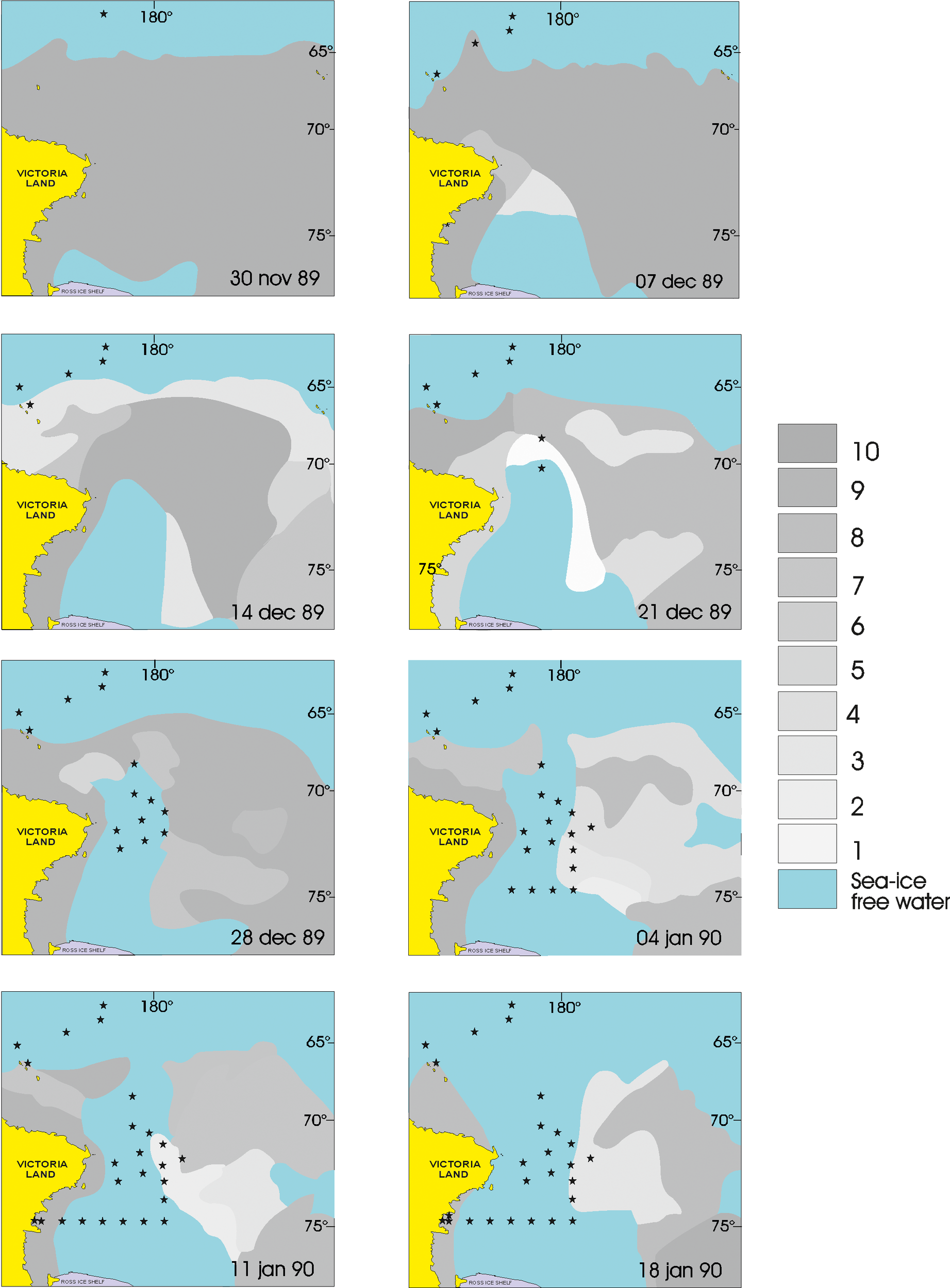
Temporal evolution of ice cover in the southern part of the studied area during the cruise period (from Hecq et al., 2000, modified). The shade of gray represents sea surface ice cover in tenths. Data are taken from satellite images published weekly by NAVY-NOAA Joint ICE Center. Stars represent the location of the BIONESS stations until the date of the image.
Figure 2
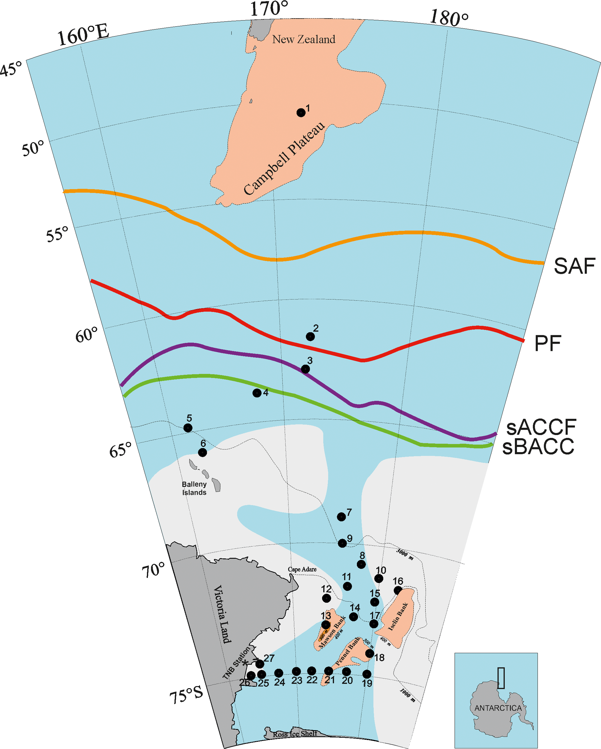
Map of study area in the Southern Pacific Ocean with ice edge extension during the cruise (from Hecq et al., 1993, modified). Location of sampling stations during the Vth ItaliAntartide Expedition (1989-1990) and fronts (SAF, Sub-Antarctic Front); PF, Polar Front; sACCF, southern Antarctic Circumpolar Current Front; sBACC, southern Boundary Antarctic Circumpolar Current (from Tesi et al., 2012 and Chapman, et al., 2020, modified).
2.2 Macrozooplankton sampling and processing
An interdisciplinary study of the Ross Sea ecosystem was undertaken during the Vth ItaliaAntartide Expedition on board the R/V Cariboo (Guglielmo et al., 1992). Between 25 November 1989 and 12 January 1990, 27 stations were sampled in the Pacific sector of the Southern Ocean, from New Zealand to the Western Ross Sea, across the Antarctic Convergence (Figure 2). Zooplankton was collected over several depth-layers, from the surface to near the seabed (Table 1), by BIONESS (Bedford Institute of Oceanography Net Environmental Sampling System), equipped with ten black nets of 500 μm mesh size (0.25 m2 mouth area; Sameoto et al., 1980). An altimeter PSA-900 (Benthos Inc.) provided information on the real-time distance to the bottom. At each sampling station, a multiparametric probe SBE 911plus (Sea-Bird Scientific, Bellevue, WA USA), which was mounted on the BIONESS frame, recorded vertical profiles of temperature (°C), salinity, and fluorescence (µg L−1 Chl a). The BIONESS was deployed at low speed along an oblique path to the maximum selected depth to be investigated, then towed at a speed of 1.5–2 m s-1 until closing, with the simultaneous opening of a new net. At almost all stations, two vertical profiles were undertaken, one from the maximum depth up to 100–200 m and the other over the depth of the euphotic layer. Depths for the euphotic layer samples were chosen according to the thermohaline structure and the fluorescence profiles. The depths of the sampled strata depended on the bottom depth (Table 1). Fishing upward, the nets were opened and closed on command, between 10–20 and 200 m intervals. Due to differences in depth at the sampling sites it was not always possible to collect the same number of samples. The volume of water filtered for each layer varied between 43 and 372 m3, according to the thickness of the sampled layer. A total of 410 samples was collected, with a total volume of 32684 m3 of water filtered. The zooplankton samples collected at each station from the surface to the maximum sampled depth, during the downward deployment of the BIONESS, were not used for this work but observed in the laboratory for the detection of rare species. On board, all the zooplankton samples were preserved in a 4% buffered formaldehyde-seawater solution.
Table 1
| Station | Date | Start | End | Local time | Depth (m) | Samples | ||||||
|---|---|---|---|---|---|---|---|---|---|---|---|---|
| Lat (° S) | Long (° E) | Lat (° S) | Long (° E) | Start | End | Bottom | Bioness haul | |||||
| 1 | 25-Nov-89 | 50.9222 | 172.0011 | 50.9717 | 171.9278 | 15.48 | 16.41 | 517 | 400 | 9 | ||
| 2 | 29-Nov-89 | 61.9956 | 172.1753 | 61.9564 | 172.2892 | 9.27 | 10.58 | 4230 | 1000 | 9 | ||
| 3 | 1-Dec-89 | 63.0764 | 171.9894 | 63.1253 | 171.9217 | 8.47 | 9.55 | 2150 | 800 | 16 | ||
| 4 | 3-Dec-89 | 63.9489 | 168.1203 | 63.9494 | 168.0375 | 21.21 | 22.40 | 3125 | 1000 | 9 | ||
| 5 | 5-Dec-89 | 64.8675 | 161.8367 | 64.8944 | 161.9778 | 10.38 | 12.10 | 3130 | 1000 | 9 | ||
| 6 | 6-Dec-89 | 66.0872 | 163.6733 | 66.0986 | 163.5508 | 16.37 | 17.25 | 2700 | 1000 | 9 | ||
| 7 | 17-Dec-89 | 69.5917 | 176.4111 | 68.6056 | 176.4389 | 17.48 | 18.17 | 3505 | 200 | 13 | ||
| 9 | 21-Dec-89 | 70.2083 | 176.4528 | 70.1667 | 176.3556 | 13.13 | 14.37 | 3285 | 1000 | 16 | ||
| 8 | 22-Dec-89 | 70.7000 | 178.1083 | 70.6750 | 178.1583 | 8.06 | 8.45 | 3350 | 200 | 16 | ||
| 10 | 23-Dec-89 | 71.2194 | 179.6806 | W | 71.1917 | 179.7472 | W | 15.02 | 15.47 | 1325 | 200 | 16 |
| 11 | 24-Dec-89 | 71.6139 | 176.8917 | 71.6361 | 176.9222 | 16.40 | 17.18 | 940 | 200 | 15 | ||
| 12 | 25-Dec-89 | 72.1667 | 173.9611 | 72.1667 | 173.9750 | 14.34 | 15.08 | 685 | 200 | 14 | ||
| 13 | 26-Dec-89 | 73.1444 | 174.4028 | 73.1750 | 174.3972 | 8.22 | 9.09 | 315 | 280 | 18 | ||
| 14 | 27-Dec-89 | 72.7333 | 177.5167 | 72.7500 | 177.4361 | 8.18 | 8.59 | 1575 | 200 | 16 | ||
| 15 | 28-Dec-89 | 72.3333 | 179.9111 | 72.3500 | 179.8889 | 8.21 | 8.55 | 2120 | 200 | 16 | ||
| 16 | 29-Dec-89 | 71.9500 | 177.7472 | W | 71.9556 | 177.7944 | W | 8.17 | 8.53 | 760 | 200 | 16 |
| 17 | 30-Dec-89 | 73.1694 | 179.9722 | W | 73.1694 | 179.9583 | W | 9.02 | 9.47 | 535 | 450 | 18 |
| 18 | 31-Dec-89 | 73.9778 | 179.9333 | 73.9917 | 179.9722 | 8.25 | 8.54 | 280 | 250 | 18 | ||
| 19 | 1-Jan-90 | 75.0056 | 179.9778 | 75.0361 | 179.8917 | W | 10.35 | 11.33 | 460 | 400 | 18 | |
| 20 | 2-Jan-90 | 74.9889 | 177.4917 | 75.0056 | 177.5389 | 8.15 | 8.47 | 390 | 350 | 18 | ||
| 21 | 3-Jan-90 | 74.9861 | 175.0000 | 75.0028 | 175.0306 | 8.22 | 8.58 | 300 | 250 | 18 | ||
| 22 | 4-Jan-90 | 74.9833 | 172.4722 | 75.0361 | 172.5333 | 8.11 | 9.19 | 545 | 500 | 16 | ||
| 23 | 5-Jan-90 | 75.0028 | 169.9556 | 74.9750 | 170.0778 | 8.24 | 9.09 | 345 | 300 | 18 | ||
| 24 | 6-Jan-90 | 74.9972 | 167.5500 | 74.9833 | 167.3833 | 8.28 | 9.27 | 520 | 450 | 18 | ||
| 25 | 7-Jan-90 | 74.9389 | 165.4000 | 74.9889 | 165.3111 | 12.20 | 13.51 | 885 | 800 | 15 | ||
| 26 | 8-Jan-90 | 74.9528 | 164.1444 | 74.9528 | 164.3139 | 14.59 | 15.57 | 635 | 450 | 18 | ||
| 27 | 12-Jan-90 | 74.7667 | 164.9861 | 74.7889 | 164.8250 | 11.01 | 12.10 | 735 | 600 | 18 | ||
Station data for BIONESS zooplankton samples taken during the Vth ItaliAntartide Expedition (1989-1990) in the Pacific sector of Southern Ocean.
In the laboratory all amphipods were counted and removed, fixed in 70% ethyl alcohol and identified to species level based on the taxonomic keys provided by Bowman (1973, 1978), Bowman and Gruner (1973); Shih (1991); Vinogradov et al. (1996), and Zeidler (1999, 2003, 2004a, 2004b, 2009, 2012a, 2012b, 2015, 2016) and classified in accordance with Lowry and Myers (2017). Taxonomic names were verified against the World Register of Marine Species (WoRMS) (Horton et al., 2019). All occurrence records at the subspecies level, synonyms, and misspellings were corrected to the valid species name and included.
Subsamples (1 to 10 mL) were extracted by Stempel pipette and observed under a Leica Wild M10 stereomicroscope for the determination of mesozooplankton abundance. The abundance of amphipods in each stratum was calculated by dividing the total number (N) by the volume of filtered water and expressed as individuals 100 m-3. For the entire water column, the total abundance of amphipods at each station was expressed as a weighted mean, summing all counted amphipods and dividing by the total of seawater filtered volume (m3), then multiplied by the water column thickness and expressed as individuals m-2. The mean total abundance of a given species is represented by the geometric mean and expressed as individuals m-2, to minimize the difference in water column depth.
Using the Seabird CTD profiles potential temperature (θ, °C) and potential density anomaly (σ0, kg m-3) were calculated and plotted with Ocean Data View software (Schlitzer, 2023). Flow velocity and filtration efficiency were monitored by internal and external TSK flowmeters.
2.3 Diversity and species assemblages
Species richness R and genus richness D for amphipods were calculated for each station and used to summarize their diversity over the sampling region (Burridge et al., 2017).
To gain insight into the underlying causes of the latitudinal trends in species richness, a partitioning clustering method named k-means algorithm (Jain and Dubes, 1988) was used to classify observations and distinguish the spatial distribution of different groups or clusters. It classifies objects into multiple groups, so that objects within the same cluster are as similar as possible. Since the number of clusters (k) was not known a priori, a preliminary analysis was performed to evaluate the partitioning of the observations between the different clusters, considering a number of clusters between 2 and 10. For each k value, 10 iterations were performed, starting from random initial positions for the k centers and taking into account the relative average values obtained. To further evaluate how many clusters to consider when determining an optimal solution, internal validity indexes were applied. In particular, the indices used by Giacalone et al. (2022) were considered (Table 2), using the NBClust package (Charrad et al., 2014) in the R statistical environment (R Core Team, 2020).
Table 2
| Index name | Cluster |
|---|---|
| “kl” (Krzanowski and Lai, 1988) | 9 |
| “ch” (Calinski and Harabasz, 1974) | 9 |
| “hartigan” (Hartigan, 1975) | 10 |
| “cindex” (Hubert and Levin, 1976) | 3 |
| “db” (Davies and Bouldin, 1979) | 8 |
| “silhouette” (Rousseeuw, 1987) | 2 |
| “duda” (Duda and Hart, 1973) | 3 |
| “beale” (Beale, 1969) | 3 |
| “ratkowsky” (Ratkowsky and Lance, 1978) | 7 |
| “ball” (Ball and Hall, 1965) | 3 |
| “gap” (Tibshirani et al., 2001) | 2 |
| “mcclain” (McClain and Rao, 1975) | 2 |
| “sindex” (Halkidi et al., 2000) | 6 |
| “sdbw” (Halkidi et al., 2001) | 6 |
| “ptbiserial” (Milligan, 1980, 1981) | 8 |
Indexes used to evaluate the clusters number (Charrad et al., 2014), with the number of cluster obtained.
The factoextra package in R was used for carrying out the cluster analysis through k-means. Once the number of clusters was identified, the main species that were more abundant in the study area were analyzed and boxplots were generated to illustrate their abundance and distribution within the identified clusters.
Relationships between the amphipod communities and environmental variables at the sampling stations were explored using a combination of non-metric multidimensional scaling (NMDS), an ordination method that can summarize relationships into 2-dimensional space and an Envfit function that fits environmental vectors or factors onto an ordination. For this a R’s Vegan package was used (Oksanen et al., 2017). To perform the NMDS analysis, the environmental data and species abundances were grouped in three sub-layers, that were chosen based on the physical features of the stations. The distance matrix used in the NMDS was the Bray-Curtis similarity index. The dataset was square-root transformed and standardized by means of the Wisconsin method before computing the distance matrix. The square-root transformation was used to downweight the importance of very abundant species, while the Wisconsin standardization (performing a double standardization in terms of species maxima and layer abundance) enabled the highlighting of the differences between layers. The performance of the ordination was evaluated by looking at the stress coefficient, where stress values higher than 0.2 highlight poor NMDS performance (Clarke, 1993) and results should be interpreted with caution.
3 Results
3.1 Environmental parameters
The analysis of the hydrological characteristics of the 27 CTD stations provided evidence for the presence of several water masses. The potential temperature (θ in °C) and salinity (S) measurements obtained from CTD casts were used to construct the θ/S diagrams (Figures 3A, B), where the dashed line indicates the surface freezing point (Tf, Figure 3A). All waters with σ0 less than 27.55 kg m-3 can be generically encompassed under the definition of Antarctic Surface Water (AASW), in agreement with Bergamasco et al. (2002). This water mass occupies the upper ocean and is significantly affected by surface processes such as cooling/heating, air temperature, wind and precipitation (Wang et al., 2023).
Figure 3
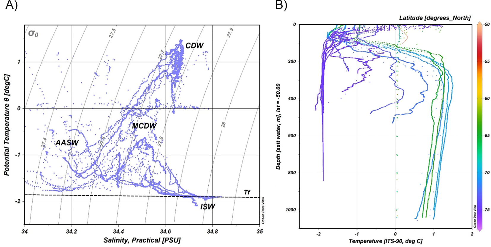
(A) θ/S characteristics from the 27 hydrological stations. The diagram is supplemented by isopycnals (σ0) and freezing temperature (Tf) relative to sea surface pressure. The dashed line indicates the surface freezing point (Tf). The main water masses are labelled with ISW (Ice Shelf Water), MCDW (Modified Circumpolar Deep Water), AASW (Antarctic surface water) and CDW (Circumpolar Deep Water). (B) Temperature profiles of the 27 hydrological stations; the color of each profile is linked to the latitude of each station.
Temperatures higher than 1.0 °C are typical of the stations dominated by Circumpolar Deep Water (CDW; Bergamasco et al., 2002). The CDW signal was identified at some CTD stations (4, 5, 8, 9, 10, 11, 14 and 15 in Figure 1) by the typical bell shape with temperatures higher than 1.0 °C between 200 m and 850 m (Figures 4 and 5). According to Orsi and Wiederwohl (2009), some CDW continues poleward and enters the cyclonic circulation of the Ross Gyre, entrenched between the colder AASW above and the Antarctic Bottom Water below (Orsi et al., 1999). During the survey this structure in the water masses was observed in the stations 8, 9, 10 and 11. The Modified Circumpolar Deep Water (MCDW) originates from CDW and is modified by cooling and mixing with shelf waters (Wang et al., 2023). It is defined by temperatures up to -1.0 °C at the shelf-break (Jacobs et al., 1985) and was observed at CTD stations 12, 13, 17, 19, 20 and 21. The waters with temperatures below the sea surface freezing point (Tf) define the Ice Shelf Water (ISW; Jacobs et al., 1985). ISW found on the continental shelf (stations 25, 26 and 27) had salinities around 34.7 and minimum temperatures reaching down to -2.08 °C, values which agree well with previous observations (Gouretskvi, 1999).
Figure 4
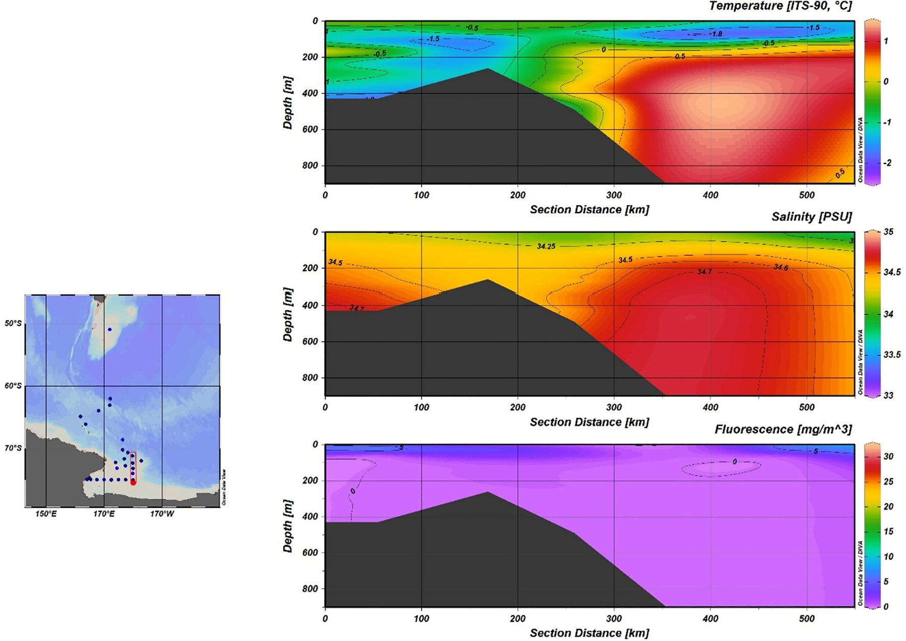
Temperature, salinity and fluorescence distribution along the S-N section including CTD Stations 10, 15, 17, 18, 19.
Figure 5
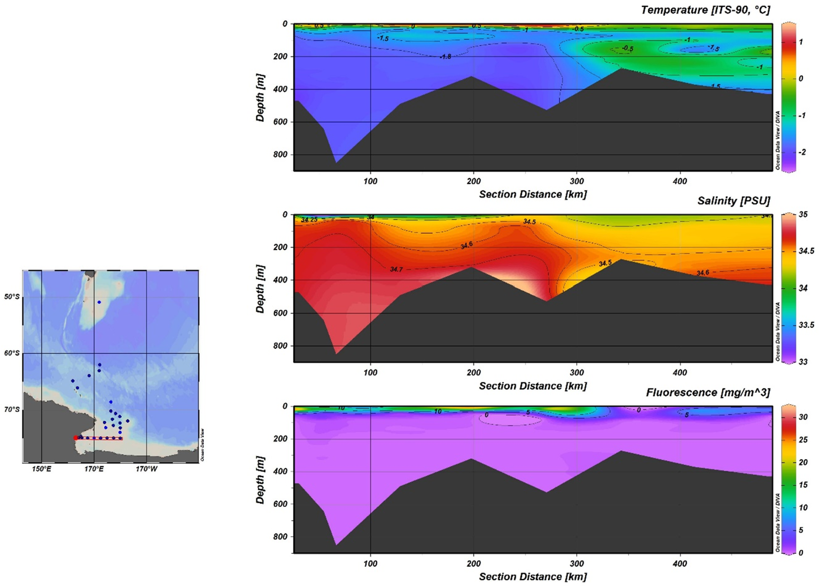
Temperature, salinity and fluorescence distribution along the W-E section including CTD Stations 19, 20, 21, 22, 23, 24, 25, 26.
Fluorescence profiles show the presence of DCM (Deep Chlorophyll Maxima) at depths between 10 m and 28 m. The comparison of chlorophyll values (as a proxy of primary production), recorded in the S-N (Figure 4) and W-E (Figure 5) sections, shows that the innermost area of the Ross Sea is characterized by higher productivity.
3.2 Zooplankton community
Mean total zooplankton abundance across the 27 sampled stations was in the range 1392.27 ± 2457.23 ind. 100 m-3. Copepoda was the most abundant taxon, representing 79.3% of total zooplankton (total weighted mean abundance 1103.76 ± 1943.43 ind. 100 m-3), followed by Chetognatha (65.49 ± 85.27 ind. 100 m-3, 4.7%), Euphausiacea (44 ± 152.46 ind. 100 m-3, 3.2%), Pteropoda (32.93 ± 49.83 ind. 100 m-3, 2.4%), Ostracoda (32.98 ± 36.34 ind. 100 m-3, 2.4%), Polychaeta (34.46 ± 185.74 ind. 100 m-3, 2.5%), Salpida (20.69 ± 120.17 ind. 100 m-3, 1.5%) and fish larvae (13.96 ± 67.2 ind. 100 m-3, 1%). All the other taxa represented less than 1% each and together accounted for 5.4%.
3.3 Amphipod diversity and abundance
A total of 2058 pelagic amphipods were observed for the study region, representing 0.4% of the total zooplanktonic community abundance. Overall, 24.8% samples (106 out of 410) did not contain amphipod specimens, regardless of the filtered water volume. The total amphipod abundance was 925.6 ind. m-2 and the mean abundance among the 27 sampling stations was 34.3 ind. m-2 (± 33.6 ind. m-2). Forty-three taxa were recovered in the investigated area (Table 3), that belonged to 18 families of amphipods and to 2 suborders. Twenty-seven species (belonging to 15 families), twelve genera (belonging to 8 families) and one taxon at family level (Phoxocephalidae) were identified.
Table 3
| Suborder | Family/Species | Abundance | Percent | N | Frequency |
|---|---|---|---|---|---|
| ind m-2 | % | % | |||
| Amphilochidea | Cyphocarididae Lowry & Stoddart, 1997 | ||||
| Cyphocaris richardi Chevreux, 1905 | 0.06 | 0.2 | 2 | 11.1 | |
| Epimeriidae Boeck 1871 | |||||
| Epimeria (Epimeriella) macronyx (Walker, 1906) | 0.84 | 2.5 | 47 | 25.9 | |
| Eusiridae Stebbing, 1888 | |||||
| Cleonardo longipes Stebbing, 1888 | 0.02 | 0.1 | 1 | 3.7 | |
| Eusirus microps Walker, 1906 | 0.08 | 0.2 | 5 | 11.1 | |
| Pardaliscidae Boeck, 1871 | |||||
| Halice tenella Birstein & Vinogradov, 1962 | 0.01 | 0.04 | 1 | 3.7 | |
| Phoxocephalidae | 0.02 | 0.1 | 1 | 3.7 | |
| Scopelocheiridae Lowry & Stoddart, 1997 | |||||
| Scopelocheiropsis abyssalis Schellenberg, 1926 | 0.10 | 0.3 | 1 | 3.7 | |
| Stegocephalidae Dana, 1852 | |||||
| Parandania boecki (Stebbing, 1888) | 0.09 | 0.3 | 3 | 3.7 | |
| Parandania sp. Stebbing, 1899 | 0.03 | 0.1 | 1 | 3.7 | |
| Tryphosidae Lowry & Stoddart, 1997 | |||||
| Pseudorchomene plebs Hurley, 1965 | 4.05 | 11.8 | 289 | 48.1 | |
| Pseudorchomene rossi Walker, 1903 | 0.42 | 1.2 | 32 | 37.0 | |
| Uristidae Hurley, 1963 | |||||
| Abyssorchomene scotianensis (Andres, 1983) | 0.01 | 0.04 | 1 | 3.7 | |
| Hyperiidea | Archaeoscinidae K.H. Barnard, 1930 | 0.03 | 0.1 | 1 | 3.7 |
| Archaeoscina sp. Stebbing, 1904 | 0.03 | 0.1 | 1 | 3.7 | |
| Cyllopodidae Bovallius, 1887 | |||||
| Cyllopus lucasii Spence Bate, 1863 | 0.02 | 0.1 | 1 | 3.7 | |
| Cyllopus magellanicus Dana, 1853 | 0.21 | 0.6 | 9 | 7.4 | |
| Cyllopus sp. Dana, 1852 | 0.08 | 0.2 | 3 | 7.4 | |
| Hyperiidae Dana, 1852 | 0.05 | 0.2 | 2 | 3.7 | |
| Hyperiella antarctica Bovallius, 1887 | 0.03 | 0.1 | 1 | 7.4 | |
| Hyperiella dilatata Stebbing, 1888 | 15.39 | 44.9 | 1033 | 74.1 | |
| Hyperiella macronyx Walker, 1906 | 2.77 | 8.1 | 191 | 66.7 | |
| Hyperoche capucinus Barnard, 1930 | 0.05 | 0.1 | 2 | 7.4 | |
| Hyperoche sp. Bovallius, 1887 | 0.03 | 0.1 | 1 | 3.7 | |
| Themisto abyssorum (Boeck, 1871) | 0.01 | 0.02 | 1 | 3.7 | |
| Themisto compressa Goës, 1866 | 0.22 | 0.7 | 13 | 3.7 | |
| Themisto gaudichaudii Guérin, 1825 | 0.90 | 2.6 | 36 | 11.1 | |
| Themisto sp. Guérin, 1826 | 1.02 | 3.0 | 59 | 3.7 | |
| Lanceolidae Bovallius, 1887 | 0.03 | 0.1 | 1 | 3.7 | |
| Lanceola clausii pirloti Shoemaker, 1945 | 0.02 | 0.1 | 1 | 3.7 | |
| Lanceola sp. Say, 1818 | 0.03 | 0.1 | 1 | 3.7 | |
| Scypholanceola sp. Woltereck, 1905 | 0.08 | 0.2 | 3 | 11.1 | |
| Mimoscinidae Zeidler, 2012 | |||||
| Mimoscina sp. Pirlot, 1933 | 0.17 | 0.5 | 4 | 11.1 | |
| Phronimidae Rafinesque, 1815 | |||||
| Phronima atlantica Guérin-Méneville, 1836 | 0.02 | 0.05 | 1 | 3.7 | |
| Phrosinidae Dana, 1852 | |||||
| Primno macropa Guérin-Méneville, 1836 | 4.11 | 12.0 | 169 | 74.1 | |
| Scinidae Stebbing, 1888 | |||||
| Acanthoscina sp. Vosseler, 1900 | 0.13 | 0.4 | 2 | 7.4 | |
| Ctenoscina brevicaudata Wagler, 1926 | 0.05 | 0.1 | 2 | 7.4 | |
| Ctenoscina sp. Wagler, 1926 | 0.03 | 0.1 | 1 | 3.7 | |
| Scina antarctica Wagler, 1926 | 0.31 | 0.9 | 14 | 18.5 | |
| Scina borealis (G.O. Sars, 1883) | 0.23 | 0.7 | 10 | 11.1 | |
| Scina pusilla Chevreux, 1919 | 0.12 | 0.4 | 2 | 7.4 | |
| Scina sp. Prestandrea, 1833 | 1.16 | 3.4 | 44 | 25.9 | |
| Vibiliidae Dana, 1852 | |||||
| Vibilia armata Bovallius, 1887 | 1.12 | 3.3 | 61 | 14.8 | |
| Vibilia sp. H. Milne Edwards, 1830 | 0.11 | 0.3 | 4 | 7.4 |
Amphipod species identified in the study area: total mean weighted abundance overall all stations, per cent contribution of each species, number of counted specimens (N), per cent frequency of occurrence in the sampling stations.
Hyperiella dilatata (Hyperiidae) was the most abundant species, representing 44.9% (1033 total counted specimens, 15.4 ind. m-2) of the total collected amphipods. Primno macropa and Pseudorchomene plebs represented 12% (169 total counted specimens, 4.11 ind. m-2) and 11.8% (289 total counted specimens, 4.05 ind. m-2), respectively. In decreasing order the amphipod community included Hyperiella macronyx 8.1% (191 total counted specimens, 2.77 ind. m-2), Scina sp. 3.4% (44 total counted specimens, 1.16 ind. m-2), Vibilia armata 3.3% (61 total counted specimens, 1.12 ind. m-2), Themisto sp. 3% (59 total counted specimens, 1.02 ind. m-2), Themisto gaudichaudii 2.6% (36 total counted specimens, 0.9 ind. m-2), Epimeria (Epimeriella) macronyx 2.5% (47 total counted specimens, 0.84 ind. m-2) and Pseudorchomene rossi 1.2% (32 total counted specimens, 0.42 ind. m-2). The remaining 33 identified taxa contributed less than 1% to the total amphipod abundance, although many contributed to high biodiversity. Together these rarer taxa represented 7% of the amphipod community.
3.4 Distribution patterns: horizontal distribution
Amphipods were observed at all sampling stations, though not in every sample from each station. The horizontal distribution of total amphipod abundance across the 27 stations is shown in Figure 6. Highest abundance (119.4 ind. m-2) was observed at station 25 within Terra Nova Bay and the lowest (6.73 ind. m-2) at station 14. A high abundance was also observed at station 1 at the Sub-Antarctic sampling site south of New Zealand. Amphipods were particularly abundant in the Polar Frontal Zone, both at station 2, north of the Antarctic Convergence (six identified species and four genera of unidentified species) and at the southern station 3 (seven identified species and three genera of unidentified species). The lowest amphipod richness (three species) was found at stations 12 and 18 (Figure 7).
Figure 6
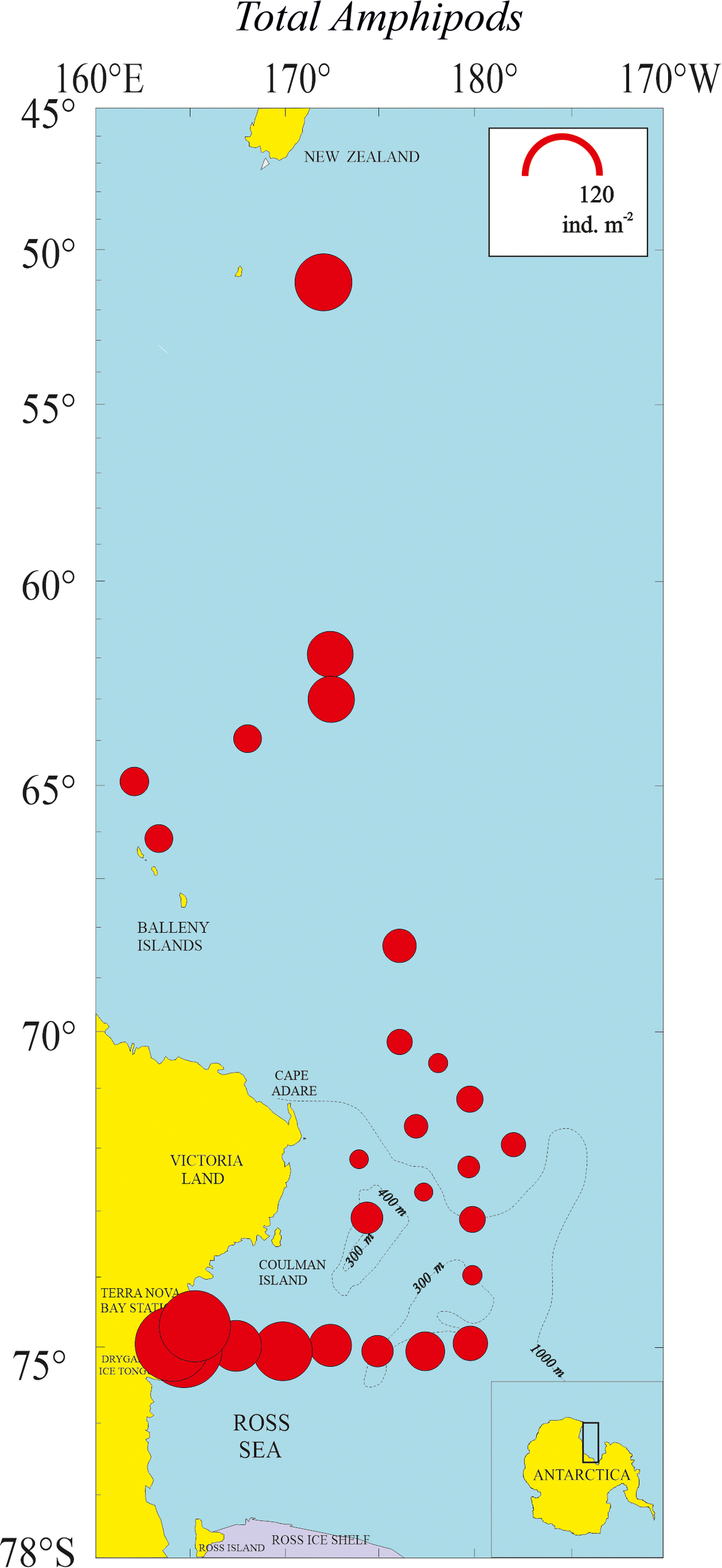
Density representation (ind m-2) of total amphipod community in the 27 sampled stations.
Figure 7
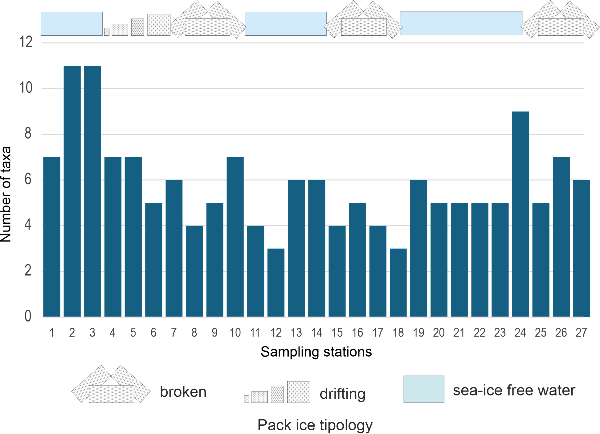
Amphipod species richness and representation of pack-ice tipology in the sampled stations.
Hyperiella dilatata and P. macropa were distributed widely (20 out of 27 sampling stations), with a percentage frequency of occurrence (PFO) of 74% (Table 3). Hyperiella macronyx (PFO = 67%) was detected at 18 sampling stations. Pseudorchomene plebs was present at 48% of the stations, followed by P. rossi (37%, 10 stations), E. (Epimeriella) macronyx and Scina sp. (7 stations), Scina antarctica (5 stations) and V. armata (4 stations). All the other identified 25 species or taxa were detected occasionally, being present at one to three stations.
The horizontal distribution of the four most abundant species is shown in Figure 8. Hyperiella dilatata had the highest abundances in the Ross Sea, particularly inside Terra Nova Bay near the coast at station 26 (90.3 ind. m-2). Primno macropa had a more pelagic distribution, starting from the eastern part of Cape Adare and the southern Pacific sector north of the Balleny Islands, with the highest abundance observed at station 7 (18.56 ind. m-2). Pseudorchomene plebs was not detected off Cape Adare going north towards New Zealand. The highest abundance was at station 20 (23.3 ind. m-2), where the juveniles (17.8 ind. m-2) were more abundant than the adults. Hyperiella macronyx showed a similar horizontal distribution to P. plebs, but with the highest abundance inside Terra Nova Bay, especially at station 27 (14.6 ind. m-2). The other six species that followed in decreasing order of abundance (see Table 3), present each one with a percent contribution between 3.4% and 1.2%, showed distinct narrow horizontal distributions. Scina sp. was absent in the Ross Sea and present only off Cape Adare going northwards; V. armata was detected at stations 1 to 5; Themisto sp. was collected at station 1, the sampling site closest to New Zealand; T. gaudichaudii was present at stations 1 to 3; E. (Epimeriella) macronyx and P. rossi were detected only in the Ross Sea and inside Terra Nova Bay.
Figure 8
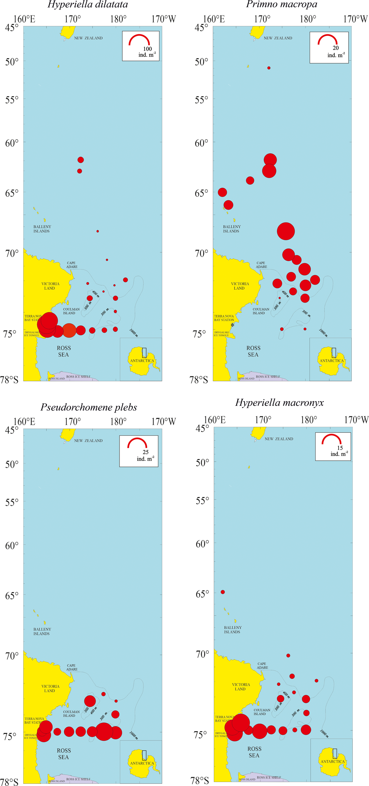
Density representation (ind m-2) of the four most abundant amphipod species (Hyperiella dilatata, Primno macropa, Pseudorchomene plebs, Hyperiella macronyx) in the 27 sampled stations.
3.5 Vertical distribution
Over the vertical plane the amphipod community mainly (75%) occupied the 20–100 m layer. The 7.3% of the community was collected in the surface layer, while 15.9% occurred between 100 and 500 m. Only 1.6% were detected in the deepest layers between 500 and 1000 m. The patterns of vertical distribution for the four most abundant species are shown in Figure 9. For H. dilatata, P. macropa and H. macronyx the abundance includes both adults and a very few juvenile specimens, while for P. plebs the two developmental stages are shown separately.
Figure 9
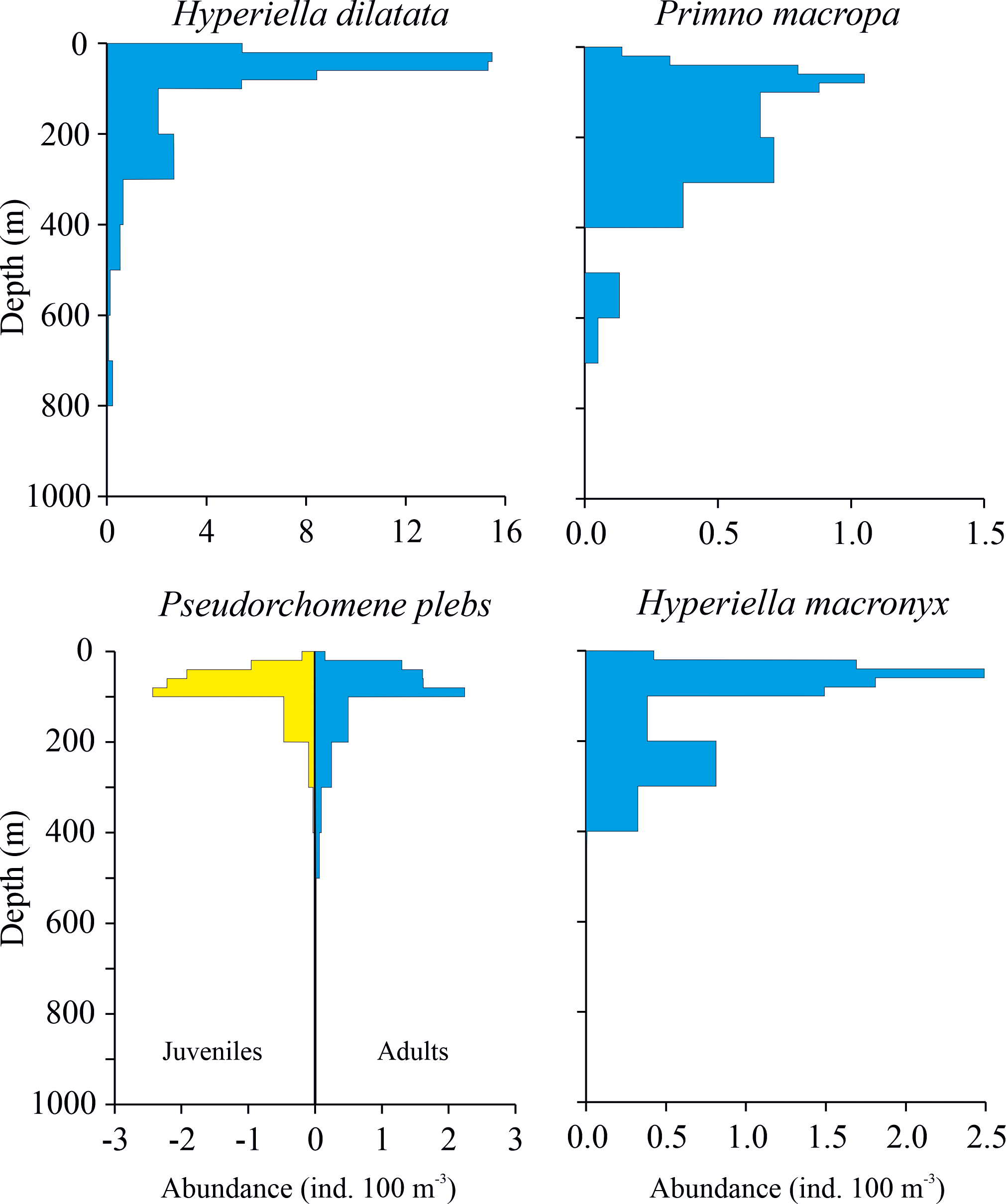
Vertical profiles of mean weighed abundance (ind. 100 m-3) for the four most abundant amphipod species (Hyperiella dilatata, Primno macropa, Pseudorchomene plebs, Hyperiella macronyx). Profiles for adults are shown. Only for P. plebs, profiles also for juvenile stages are shown. Note differences in scales on x-axis.
Hyperiella dilatata occupied the depth from 800 m to the surface, although the bulk of the population (88%) was found in the 0–100 m layer.
Primno macropa showed a more uniform distribution through the water column than H. dilatata and was collected from the surface to 700 m. The main part of the population (80%) showed a wide distribution, occupying the 40-300m depth layer. No individuals were found in the 400-500 m layer. Only six P. macropa juvenile specimens were collected, in the 300-400 m and 100-200 m layers.
Adult Pseudorchomene plebs occurred between 500 m and the surface. The main part of the adult population (87%) occupied the 20–100 m layer, while only 2% were present in the most superficial layer (0–20 m). Juvenile P. plebs were almost as abundant as adults and showed similar vertical distribution.
Hyperiella macronyx were distributed from 400 m to the surface. Approximately 80% occupied the 20–100 m layer, with ~4% in the more superficial layer and the 16% below 100 m depth. Only two juveniles were collected in the 200–300 m layer.
3.6 Latitudinal boundaries
The spatial distribution boundaries of the amphipod taxa collected during this study, are shown in Table 4. Only two species (Phronima atlantica and Themisto compressa) and one genus (Themisto sp.) were found exclusively in the Sub-Antarctic zone (station 1) at latitude 50.9222°S, while three species (Halice tenella, Hyperiella antarctica and Parandania boecki) and one family (Lanceolidae) were found only in the area north of the Polar Front (station 2, 61.9956°S). Cyllopus magellanus and T. gaudichaudii were recovered only between the Sub-Antarctic zone and Polar Front (stations 1 and 3), while Cyphocaris richardi and two genera (Cyllopus sp. and Vibilia sp.) were present only in the Polar Front (stations 2 and 3), between 61.9956 and 63.0764°S. Four genera (Archaeoscina sp., Ctenoscina sp., Lanceola sp. and Parandania sp.) were found in the area south of the Polar Front (station 4, 63.9489°S). One species (Scopelocheiropsis abyssalis), one genus (Acantoscina sp.) and one family (Archaeoscinidae) were found in the ice-covered stations 6 and/or 7. Hyperiella dilatata and H. macronyx were present throughout all the study area, including Terra Nova Bay, with a small difference in the northern limit of their detection: the Polar Front (61.9956°S) and the Balleny Islands (64.8675°S), respectively. Primno macropa was collected over a large area, from the Sub-Antarctic Front to the mid Ross Sea Region (at station 21). Some species were found only along the two transects at the northern entrance of the Ross Sea: Cleonardo longipes, Lanceola clausii pirloti and the family Phoxocephalidae were found exclusively in station 10 (71.2194°S), while Ctenoscina brevicaudata, Cyllopus lucasii and Temisto abyssorum were recorded at stations 13,14,15. Eusirus microps and Abyssorchomene scotianensis are exclusive species of Terra Nova Bay (about 75°S).
Table 4
| Amphipod species/genus/family | Area | Coordinates | Stations of detection | |||
|---|---|---|---|---|---|---|
| (latitude °S) | (longitude °E) | |||||
| from | to | from | to | |||
| Abyssorchomene scotianensis | Terra Nova Bay (TNB) | 74.9528 | 164.1444 | 26 | ||
| Acanthoscina sp. | Balleny Islands (BI)/Southern Pacific (SP) | 66.0872 | 69.5917 | 163.6733 | 176.4111 | 6,7 |
| Archaeoscina sp. | South of the Antarctic Convergence (AC) | 63.9489 | 168.1203 | 4 | ||
| Archaeoscinidae | Southern Pacific | 69.5917 | 176.4111 | 7 | ||
| Cleonardo longipes | Eastern Ross Sea (ERS) | 71.2194 | 179.6805 W | 10 | ||
| Ctenoscina brevicaudata | Western Ross Sea (WRS) | 72.3333 | 72.7333 | 177.5167 | 14,15 | |
| Ctenoscina sp. | South of the AC | 63.9489 | 168.1203 | 4 | ||
| Cyllopus lucasii | Western Ross Sea | 72.7333 | 179.9111 | 14 | ||
| Cyllopus magellanicus | Subantarctic zone/ South of the AC | 50.9222 | 63.0764 | 171.9894 | 172.0011 | 1,3 |
| Cyllopus sp. | Polar Front | 61.9956 | 172.1753 | 2,3 | ||
| Cyphocaris richardi | Polar Front | 61.9956 | 63.0764 | 171.9894 | 172.1753 | 2,3 |
| Epimeria (Epimeriella) macronyx | ERS/WRS/TNB | 71.9500 | 75.0028 | 164.1444 | 177.7472W | 16,20,23/27 |
| Eusirus microps | WRS/TNB | 74.7667 | 74.9972 | 164.1444 | 167.5500 | 24,26,27 |
| Halice tenella | North of the AC | 61.9956 | 172.1753 | 2 | ||
| Hyperiella antarctica | North of the AC | 61.9956 | 172.1753 | 2 | ||
| Hyperiella dilatata | Polar Front/SP/WRS/ERS/TNB | 61.9956 | 75.0056 | 164.1444 | 177.7472W | 2,3,7,8,12/27 |
| Hyperiella macronyx | BI/SP/WRS/ERS/TNB | 64.8675 | 75.0028 | 161.8367 | 177.7472W | 5,9,11/14,16/27 |
| Hyperiidae | South of the AC | 63.0764 | 171.9894 | 3 | ||
| Hyperoche capucinus | Southern Pacific | 69.5917 | 70.2083 | 176.4111 | 176.4528 | 7,9 |
| Hyperoche sp. | Southern Pacific | 70.7000 | 178.1083 | 8 | ||
| Lanceolidae | North of the AC | 61.9956 | 172.1753 | 2 | ||
| Lanceola clausii pirloti | Eastern Ross Sea | 71.2194 | 179.6806W | 10 | ||
| Lanceola sp. | South of the AC | 63.9489 | 168.1203 | 4 | ||
| Mimoscina sp. | Balleny Islands/Eastern Ross Sea | 64.8675 | 71.2194 | 161.8367 | 179.6806W | 5,6,10 |
| Parandania boecki | North of the AC | 61.9956 | 172.1753 | 2 | ||
| Parandania sp. | South of the AC | 63.9489 | 168.1203 | 4 | ||
| Phoxocephalidae | Eastern Ross Sea | 71.2194 | 179.6806W | 10 | ||
| Phronima atlantica | Subantarctic zone | 50.9222 | 172.0011 | 1 | ||
| Primno macropa | Everywhere except TNB | 50.9222 | 75.0056 | 161.8367 | 177.7472W | 1/17,19,21 |
| Pseudorchomene plebs | WRS/ERS/TNB | 72.7333 | 75.0028 | 164.1444 | 179.9722W | 13,14,17/27 |
| Pseudorchomene rossi | WRS/TNB | 73.1444 | 75.0056 | 164.1444 | 179.9778 | 13,19/27 |
| Scina antarctica | Balleny Islands/WRS/ERS | 64.8675 | 75.0056 | 161.8367 | 177.7472W | 5,11,15,16,19 |
| Scina borealis | South of the AC/WRS/ERS | 63.0764 | 71.6139 | 171.9894 | 179.6805W | 3,10,11 |
| Scina pusilla | Balleny Islands/ERS | 66.0872 | 71.2194 | 163.6733 | 179.6805W | 6,10 |
| Scina sp. | Polar Front/BI/Southern Pacific | 61.9956 | 70.7000 | 161.8367 | 178.1083 | 2/9 |
| Scopelocheiropsis abyssalis | Balleny Islands | 66.0872 | 163.6733 | 6 | ||
| Scypholanceola sp. | North of the AC/BI/Southern Pacific | 61.9956 | 70.2083 | 161.8367 | 176.4528 | 2,5,9 |
| Themisto abyssorum | Western Ross Sea | 73.1444 | 174.4028 | 13 | ||
| Themisto compressa | Subantarctic zone | 50.9222 | 172.0011 | 1 | ||
| Themisto gaudichaudii | Subantarctic zone/Polar Front | 50.9222 | 63.0764 | 172.1753 | 172.0011 | 1/3 |
| Themisto sp. | Subantarctic zone | 50.9222 | 172.0011 | 1 | ||
| Vibilia armata | Subantarctic zone/South of the AC/BI | 50.9222 | 64.8675 | 161.8367 | 172.0011 | 1,3/5 |
| Vibilia sp. | Polar Front | 61.9956 | 63.0764 | 171.9894 | 172.1753 | 2,3 |
Spatial distribution boundaries of identified amphipod species inside the investigated area with this study.
Boundaries of distribution as latitude °S and longitude °E are shown.
3.7 Species assemblages
The k-means algorithm, applied to species abundances estimated for the 27 stations, enabled the evaluation of the spatial distribution of different groups. To evaluate the optimal number of clusters, 15 indices were estimated (Table 2). The results of this approach revealed the presence of three clusters (Figure 10). Cluster 1 was mainly composed of the southernmost stations, Cluster 2 included the three northernmost stations, while the stations in the central part of the study area were grouped in Cluster 3 (Figure 10). The boxplots of the main species in the three clusters are shown in Figure 11.
Figure 10

Results of the cluster analysis on amphipod species collected in the 27 stations.
Figure 11
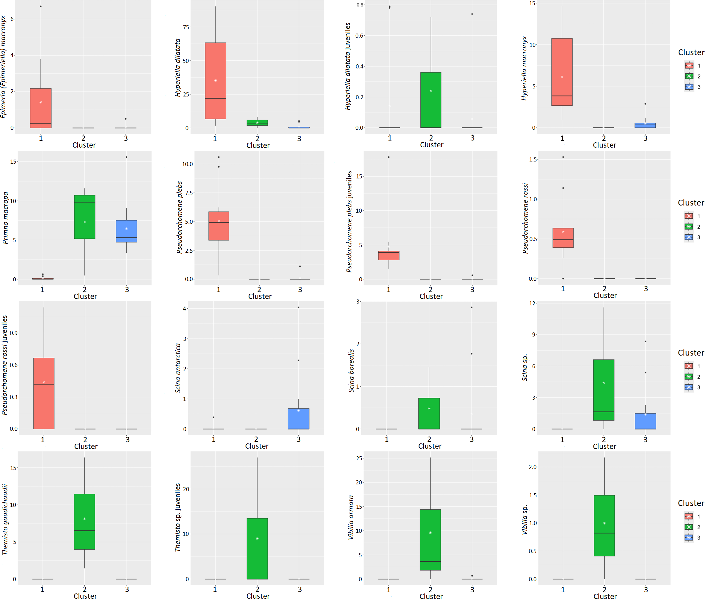
Boxplot of the main amphipod species in the three clusters.
CTD profiles belonging to Cluster 1 showed the presence of a strong chlorophyll signal, with the DCM located at around 28 m depth. Profiles belonging to cluster 2 were characterized by an almost homogeneous upper layer (0–200 m) in terms of temperature, salinity and fluorescence; for this cluster no clear DCM signal was evident. Most of the stations belonging to cluster 3 were influenced by the presence of CDW and MCDW. At these stations the presence of a DCM was less evident than in stations of cluster 1 and was located around 50 m depth.
NMDS was used to investigate the relationships between amphipod taxa and the sampling stations. The NMDS stress value was 0.11, indicating acceptable fit. The NMDS plot (Figure 12) showed a clear separation between northern and southern stations along the first NMDS axis (NMDS1). In particular, the upper layers (0–50 m and 50–200 m) of the southern stations, belonging to Cluster 1 and affected by higher fluorescence and lower temperatures, were characterized by higher proportions of H. dilatata, H. macronyx and P. plebs, while the species Epimeria (Epimeriella) macronyx was more common in the middle layer (50–200 m) in the south-western side of the Ross Sea. The deepest layer (>200 m) in these stations was characterized by a species assemblage composed of Hyperiella dilatata, H. macronyx, Pseudorchomene plebs and P. rossi. The NMDS plot also showed that the upper layers (0–50 m and 50–200 m) of the stations belonging to Cluster 3, influenced by relatively higher temperature and lower fluorescence values, were mainly characterized by higher proportions of P. macropa. Lower proportions of H. dilatata, H. macronyx and Scina sp. were also observed at a few stations in this cluster. The deepest layer (>200 m), where higher salinity was observed, was mainly characterized by the presence of P. macropa and Scina sp. Higher proportions of T. gaudichaudii, V. armata, and Vibilia sp. characterized the three northernmost stations belonging to Cluster 2. Finally, juvenile specimens of Themisto sp. were found in the upper and saltier layers of station 1.
Figure 12
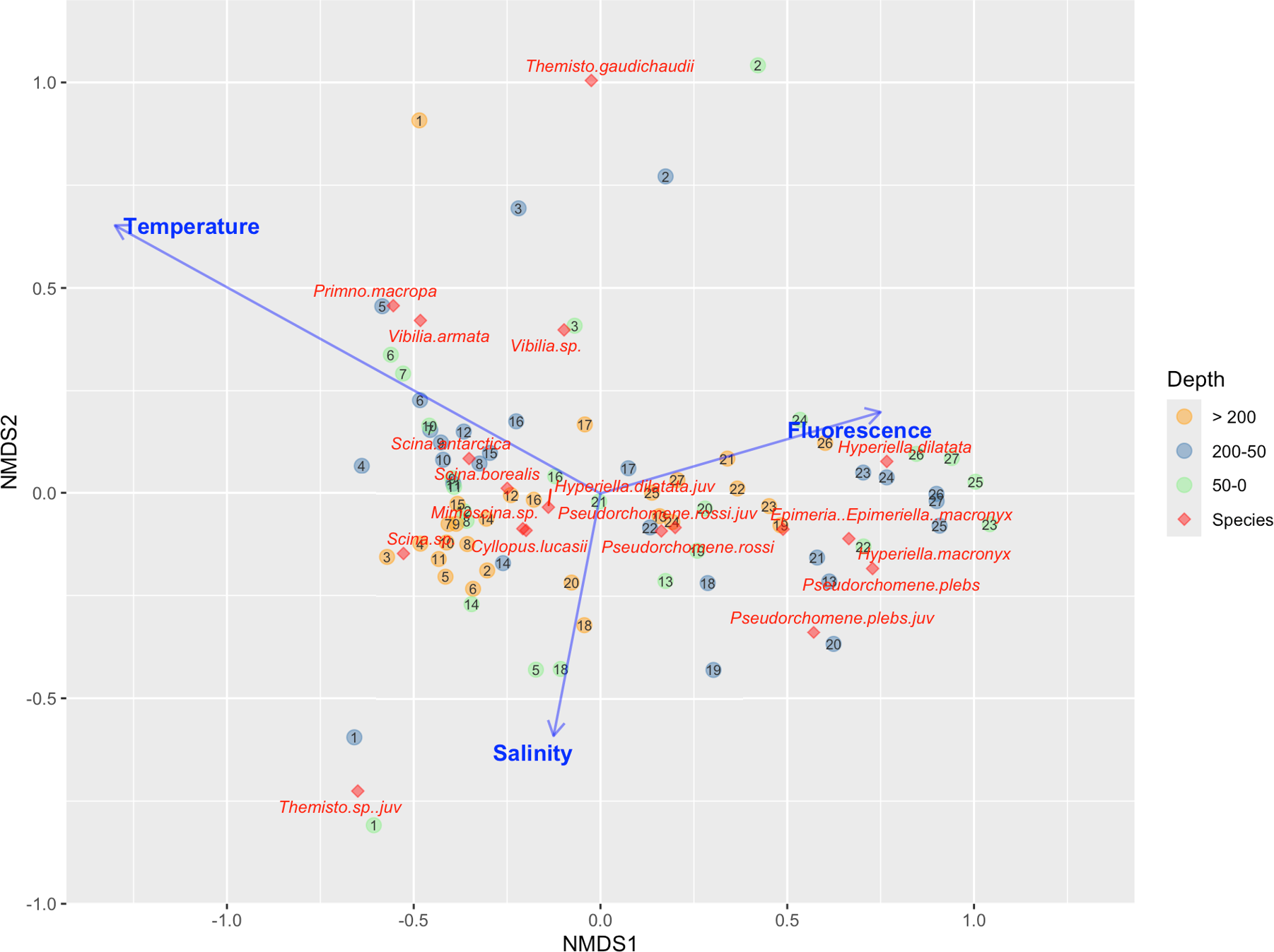
Non-metric multidimensional scaling (NMDS) ordination results, reporting the relationships among amphipods species, environmental factors (Temperature, Salinity and Fluorescence) and sampling stations. The number in each circle is the station number. Colors represent the considered layers: green for the layer 0–50 m, dark grey for the layer 50–200 m and yellow for the layer with depth > 200 m.
4 Discussion
A review of marine biodiversity in the Southern Ocean highlighted the relative importance of some zoological groups like molluscs and polychaetes, and the predominance of crustaceans (Dauby et al., 2003). Among the latter, amphipods represent the richest group, with more than 820 species recorded in the Antarctic and Sub-Antarctic regions (De Broyer and Jażdżewski, 1993, 1996). These crustaceans have colonized a wide variety of ecological niches, including benthic, pelagic and ice-habitats (De Broyer et al., 2001), and have developed a wide range of feeding strategies (Dauby et al., 2001a; Nyssen et al., 2002; Dauby et al., 2003). The faunal diversity of amphipods indicates the importance of these crustaceans to total pelagic biomass, and thus their major role in the trophodynamics of Antarctic ecosystems, both as consumers and prey. Information about the biodiversity and biogeography of Atlantic and Pacific Sectors of Southern Ocean pelagic amphipods is lacking and only available for some restricted areas including the eastern Weddell Sea and Terra Nova Bay (e.g. Gerdes et al., 1992; Minutoli et al., 2023).
In the present study high biodiversity of pelagic amphipods was observed for the Pacific sector of the Southern Ocean. A total of 43 taxa was recovered, which was more than double the 20 identified in a previous study in a more restricted area, the Ross Sea and Terra Nova Bay, during the 1987–1988 Vth ItaliaAntartide R/V Polar Queen Expedition (Minutoli et al., 2023). Only five species (Hyperiella dilatata, H. macronyx, Primno macropa, Pseudorchomene plebs, P. rossi) were common to both oceanographic campaigns. This can be linked to the wider geographic coverage of the investigated area in the present study, which covered a greater range in bathymetry and oceanography. Hyperiidea was the most represented suborder (83.3% of the collected specimens), instead the other 16.7% were Amphilochidea. Hyperiidae was the most abundant family (60%), confirming that, in the Southern Ocean, hyperiidean amphipods are particularly abundant, with distributions ranging from the Polar Frontal Zone to Antarctic shelf waters (Havermans et al., 2019). This family was represented in the present study by seven species and two genera of unidentified species, with a dominance of H. dilatata (Minutoli et al., 2023). Given its wide spatial distribution in the studied area, H. dilatata has been described as cosmopolitan in the Southern Ocean. It is common in the Pacific sector and represents the most abundant and key amphipod species in the Ross Sea food chain (Barnard, 1930; Foster, 1987; Stebbing, 1888; Weigmann-Haass, 1989; Hubold, 1992; Jażdżewski et al., 1992; Dinofrio, 1997; Guglielmo et al., 1998; Vinogradov, 1999; La Mesa et al., 2004; Guglielmo et al., 2011; Minutoli et al., 2023).
The family Tryphosidae was the second most abundant family (13%), represented by two species, of the most common which was P. plebs. Literature reports show that this species as widely distributed in the Southern Ocean and in the Ross Sea (d’Udekem d’Acoz and Havermans, 2012; De Broyer et al., 2007), confirming the observations made during the 1987–1988 study. Pseudorchomene plebs has a bentho-pelagic way of life and a diversified feeding habit. Crustacean parts have been observed frequently in their gut contents, along with remains of carrion (muscles) and diatoms (d’Udekem d’Acoz and Havermans, 2012). Swarms of P. plebs have been recorded to devour fish carcasses in three days, leaving perfectly clean skeletons (d’Udekem d’Acoz and Havermans, 2012). The family Phrosinidae was the third most abundant family (11%), represented by P. macropa only. In this study, P. macropa was present in front of Cape Adare and in the Pacific Ocean moving northwards to New Zealand. It was absent in the Ross Sea and inside Terra Nova Bay (Minutoli et al., 2023).
The combined information from the oceanographic profiles and the vertical distributions of the biological samples suggested that the water column was stratified in three main layers: the first layer (0–50 m) was mainly influenced by the possible presence of a DCM and of AASW; the second layer, covering 50–200 m, was characterized by the presence of temperature minima and by a wide range of temperature (between -1.92 °C and 1.23 °C); the third layer from 200 m to the bottom was influenced by CDW or MCDW and, at a few stations, by ISW.
Amphipod species composition differed significantly between stations. The sampling strategy, spanning both a broad spatial (from 62°S to 74°S) and a broad temporal (approximately 50 days) scale, from late austral spring to early summer, allowed us to divide the study area into zones with different hydrological characteristics and ice coverage. The three different clusters identified through the k-means algorithm based on species abundance were confirmed by the NMDS plot. In particular, a correlation between species composition and the sampled layers at the different stations was highlighted. The species composition of southernmost stations in the first cluster characterized the area starting from the innermost stations in Terra Nova Bay (75°S) across east-west stations up to 180°, where higher fluorescence values, lower temperatures in the euphotic layer (0–50 m e 50–200 m) and a clear DCM at 28 m were detected. The three northernmost stations (St.1-3) were significantly different from all other stations. In this ice free zone between the Sub-Antarctic Front and Antarctic Convergence the greatest diversity of amphipod species was found in the upper and saltier layers, with high abundance of Hyperiidae like Themisto gaudichaudii. In this area, no DCM was found in an homogeneous upper layer as temperature, salinity and fluorescence. The stations in the central part of the study area were influenced by relatively higher temperature and by lower fluorescence values in the upper layers, and higher salinity in the deepest layers below 200 m, and also by the presence of CDW and MCDW water masses. Therefore, the oceanographic and environmental constrains of the water masses, together with the pack ice coverage, have determined the different highlighted habitats suitable for pelagic amphipod species assemblages. These abiotic features of the study area should be so prioritized in future monitoring efforts in the Southern Ocean under changing climate conditions. On the other hand, it’s well known that the sea ice plays a key role in structuring Antarctic ecosystem, and especially that the ice edge influences, with a cascade effect, the phytoplankton production and the zooplankton distribution and behavior and all the trophic food web (Carli et al., 2000; Hecq et al., 2000; Lazzara et al., 2000; Zunini Sertorio et al., 2000).
Knowledge of the relationship between pelagic amphipods and annual ice in the Southern Ocean is still very limited. The finding of some species, like Eusirus antarcticus, E. perdentatus, E. microps and Cheirimedon femoratus exclusively in the innermost stations of Terra Nova Bay (Minutoli et al., 2023; this study), where ice shelves along the coastline play an important role in the dynamics of Terra Nova Bay (Frezzotti, 1993), confirms the affinity of the above cited species for sea ice, as previously recorded during under‐ice dives of the Weddell Sea and the Lazarev Sea (Krapp et al., 2008). Different for pelagic swimmer amphipods, as Hyperidae and Scinidae, that were routinely sampled in multinet hauls, isolated or few individuals of the above-mentioned species have been sampled (Minutoli et al., 2023; this study). According to Krapp et al. (2008), it would be advisable to use scuba or suitable tools for sampling zooplankton in the lower part of the pack-ice to obtain better estimates of biomass and improve our information on the habits of these species.
The finding of the three species of Hyperiella confirms that this genus is endemic to the Southern Ocean, found generally south of 55°S (Zeidler and De Broyer, 2009, 2014). In this study, H. antarctica was collected between the Sub-Antarctic and the Antarctic Polar Front, confirming previous studies (Zeidler and De Broyer, 2009, 2014) and highlighting a lesser affinity to sea ice than its congeners (Flores et al., 2011). The highest abundances of H. macronyx and H. dilatata recorded in this study throughout the entire Ross Sea, and particularly inside Terra Nova Bay, may be explained by their affinity to colder waters and ice conditions. Weigmann-Haass (1989) recorded H. dilatata as relatively common around the tip of the Antarctic Peninsula and in the Weddell Sea.
5 Conclusions
The species composition, the abundance and the spatial distribution of amphipod crustaceans is of interest because they play a crucial role in ecosystems as a link between lower and higher trophic levels, and benthic-pelagic communities (Michel et al., 2016; Griffiths et al., 2017). Knowledge of the relationship between pelagic amphipods and annual ice in the Southern Ocean is still very limited. The large spatial scale investigated in this study gave us the opportunity to increase the state of knowledge on biodiversity and distribution of pelagic amphipods in the Pacific sector of the Southern Ocean. It has been proposed that pelagic species are more widespread than benthic species because of their mobility and relative homogeneity of their habitat (Costello et al., 2017). The much higher species richness found in the suborder Hyperidea (28) than in the suborder Amphilochidea (11) reflect the different investigated habitats, more ice-free pelagic waters than those covered by pack-ice. Despite only 3% of amphipod species are pelagic (Arfianti et al., 2018), this difference in biodiversity found between the two above cited suborders, could be justified by the behavior of these pelagic crustaceans that avoid predation in open pelagic waters by being relatively transparent, living within gelatinous zooplankton, having good eyesight, and being agile swimmers. Statistical analyses confirmed that sea-ice extension, water masses structure, physical and biological constraints, like water temperature, salinity and fluorescence (DCM) controlled the horizontal and vertical distribution of pelagic amphipod habitat and relative trophic behavior.
Amphipods are important in the Antarctic food chain, yet we have little knowledge of how alterations in environmental parameters linked to climate changes will influence plankton communities, particularly species distribution, life cycles and development (Beaugrand, 2009; Weydmann et al., 2018; Schröter et al., 2019). Knowledge of amphipod biodiversity by means of this study can represent a baseline for future studies. The comparison with newly collected samples may provide evidence of changes due to environmental alternations.
Statements
Data availability statement
The raw data supporting the conclusions of this article will be made available by the authors, without undue reservation.
Author contributions
RM: Conceptualization, Writing – original draft, Writing – review & editing. LG: Conceptualization, Writing – original draft, Writing – review & editing. AB: Formal Analysis, Writing – original draft. SG: Formal Analysis, Writing – original draft. RF: Formal Analysis, Writing – original draft. DD: Formal Analysis, Methodology, Writing – original draft. MG: Formal Analysis, Methodology, Writing – original draft. YG: Methodology, Writing – original draft. KS: Writing – review & editing. AG: Conceptualization, Supervision, Writing – original draft, Writing – review & editing. SA: Conceptualization, Supervision, Writing – original draft, Writing – review & editing.
Funding
The author(s) declare that financial support was received for the research, and/or publication of this article.
Acknowledgments
Logistical and financial support for this paper was given by the Italian National Program of Research in Antarctica (PNRA). A special thank goes to prof. Giuseppe Costanzo from University of Messina, teacher and mentor, who has devoted much of his life to scientific research on zooplankton taxonomy and ecology. Many thanks go to officers and crew of the research vessel R/V Cariboo and to technicians involved in the BIONESS sampling procedures for their excellent cooperation in field work. Authors would like to thank the two referees that have contributed to improve significatively the manuscript during the revision process.
Conflict of interest
The authors declare that the research was conducted in the absence of any commercial or financial relationships that could be construed as a potential conflict of interest.
The author(s) declared that they were an editorial board member of Frontiers, at the time of submission. This had no impact on the peer review process and the final decision.
Generative AI statement
The author(s) declare that no Generative AI was used in the creation of this manuscript.
Any alternative text (alt text) provided alongside figures in this article has been generated by Frontiers with the support of artificial intelligence and reasonable efforts have been made to ensure accuracy, including review by the authors wherever possible. If you identify any issues, please contact us.
Publisher’s note
All claims expressed in this article are solely those of the authors and do not necessarily represent those of their affiliated organizations, or those of the publisher, the editors and the reviewers. Any product that may be evaluated in this article, or claim that may be made by its manufacturer, is not guaranteed or endorsed by the publisher.
References
1
Arfianti T. Wilson S. Costello M. J. (2018). Progress in the discovery of amphipod crustaceans. PeerJ6, e5187. doi: 10.7717/peerj.5187
2
Arndt C. Swadling K. M. (2006). Crustacea in Arctic and Antarctic sea ice: distribution, diet and life history strategies. Adv. Mar. Biol.51, 197–315. doi: 10.1016/S0065-2881(06)51004-1
3
Ball G. Hall D. (1965). “ ISODATA,” in A Novel Method of Data Analysis and Pattern Classification (Menlo Park, California: Stanford Research Institute).
4
Barnard K. H. (1930). Crustacea. Part XI: Amphipoda. British Antarctic (Terra Nova) Expedition 1910. Zoology8, 307–454.
5
Beale E. M. L. (1969). Euclidean Cluster Analysis (London, UK: Scientific Control Systems Limited).
6
Beaugrand G. (2009). Decadal changes in climate and ecosystems in the North Atlantic Ocean and adjacent seas. Deep Sea Res. Part II56, 656–673. doi: 10.1016/j.dsr2.2008.12.022
7
Bergamasco A. Defendi V. Zambianchi E. Spezie G. (2002). Evidence of dense water overflow on the Ross Sea shelf-break. Antarct. Sci.14, 271–277. doi: 10.1017/S0954102002000068
8
Bowman T. E. (1973). Pelagic amphipods of the genus Hyperia and closely related genera (Hyperiidea: Hyperiidae). SM. C. Zool.136, 1–76. doi: 10.5479/si.00810282.136
9
Bowman T. E. (1978). Revision of the pelagic amphipod genus Primo (Hyperiidea: Phrosinidae). SM. C. Zool275, 123. doi: 10.5479/si.00810282.275
10
Bowman T. E. Gruner H. E. (1973). The families and genera of Hyperiidea (Crustacea: Amphipoda). SM. C. Zool146, 164. doi: 10.5479/si.00810282.146
11
Burridge A. Tump M. Vonk R. Goetze E. Peijnenburg K. C. (2017). Diversity and distribution of hyperiid amphipods along a latitudinal transect in the Atlantic Ocean. Progr. Oceanogr.158, 224235. doi: 10.1016/j.pocean.2016.08.003
12
Calinski T. Harabasz J. (1974). A dendrite method for cluster analysis. Commun. Stat.3, 1–27. doi: 10.1080/03610927408827101
13
Carli A. Pane L. Stocchino C. (2000). “ “Planktonic copepods in Terra Nova Bay (Ross Sea): distribution and relationship with environmental factors”,” in Ross Sea Ecology. Eds. FarandaF.GuglielmoL.IanoraA. ( Springer, Berlin Heidelberg New York), 309–322.
14
Castellani G. Schaafsma F. L. Arndt S. Lange B. A. Peeken I. Ehrlich J. et al . (2020). Large-scale variability of physical and biological sea-ice properties in polar oceans. Front. Mar. Sci.7. doi: 10.3389/fmars.2020.00536
15
Charrad M. Ghazzali N. Boiteau V. Niknafs A. (2014). NbClust: an R package for determining the relevant number of clusters ina data set. J. Stat. Softw.6, 1–36. doi: 10.18637/jss.v061.i06
16
Clarke K. R. (1993). Non-parametric multivariate analyses of changes in community structure. Aust. J. Ecol.18, 117–143. doi: 10.1111/j.1442-9993.1993.tb00438.x
17
Costello M. J. Tsai P. Wong P. S. Cheung A. K. L. Basher Z. Chaudhary C. et al . (2017). Marine biogeographic realms and species endemicity. Nat. Commun.8, 1057. doi: 10.1038/s41467-017-01121-2
18
d’Udekem d’Acoz C. D. Havermans C. (2012). Two new Pseudorchomene species from the Southern Ocean, with phylogenetic remarks on the genus and related species (Crustacea: Amphipoda: Lysianassoidea: Lysianassidae: Tryphosinae). Zootaxa3310, 1–50. doi: 10.11646/zootaxa.3310.1.1
19
Dauby P. Nyssen F. De Broyer C. (2003). “ “Amphipods as food sources for higher trophic levels in the Southern Ocean: a synthesis”,” in Antarctic Biology in a Global Context. Eds. HuiskesA. H. L.GieskesW. W. C.RozemaJ.SchornoR. M. L.Van Der ViesS. M.WolffW. J. ( Backhuys Publishers, Leiden, The Netherlands), 129–134.
20
Dauby P. Scailteur Y. Chapelle G. De Broyer C. (2001b). Potential impact of the main benthic amphipods on the eastern Weddell Sea shelf ecosystem (Antarctica). Polar Biol.24, 657–662. doi: 10.1007/s003000100265
21
Dauby P. Scailteur Y. De Broyer C. (2001a). Trophic diversity within the eastern Weddell Sea amphipod community. Hydrobiologia443, 69–86. doi: 10.1023/A:1017596120422
22
Davies D. L. Bouldin D. W. (1979). A cluster separation measure. IEEE Trans. Pattern Anal. Mach. Intell.1, 224–227. doi: 10.1109/TPAMI.1979.4766909
23
De Broyer C. Danis B. (2011). How many species in the Southern Ocean? Towards a dynamic inventory of the Antarctic marine species. Deep-Sea Res. Part II58, 5.17. doi: 10.1016/j.dsr2.2010.10.007
24
De Broyer C. Jażdżewska A. (2014). “ “Biogeographic patterns of southern ocean benthic amphipods”,” in Biogeographic Atlas of the Southern Ocean. Eds. De BroyerC.KoubbiP.GriffithsH. J.RaymondB.d’Udekem d’AcozC.Van De PutteA.DanisB.DavidB.GrantS.GuttJ.HeldC.HosieG.HuettmannF.PostA.Ropert-CoudertY. ( Scientific Committee on Antarctic Research, Cambridge), 155–165.
25
De Broyer C. Jażdżewski K. (1993). Contribution to the marine biodiversity inventory. A checklist of the Amphipoda (Crustacea) of the Southern Ocean. Doc. Trav. Inst. R. Sci. Nat. Belg.73, 1–155.
26
De Broyer C. Jażdżewski K. (1996). Biodiversity of the Southern Ocean: towards a new synthesis for the Amphipoda (Crustacea). Boll. Mus. civ. Sta. Nat. Verona20, 547–568.
27
De Broyer C. Lowry J. K. Jażdżewski K. Robert H. (2007). “ “Catalogue of the Gammaridean and Corophiidean Amphipoda of the Southern Ocean with distribution and ecological data”,” in Census of Antarctic Marine Life: Synopsis of the Amphipoda of the Southern Ocean, Vol 1. Ed. De BroyerC. ( Bull. Inst. R. Sc. N. Belgique, Biologie, Brussel), 1–325.
28
De Broyer C. Scailteur Y. Chapelle G. Rauschert M. (2001). Diversity of epibenthic habitats of gammaridean amphipods in the eastern Weddell Sea. Polar Biol.24, 744–753. doi: 10.1007/s003000100276
29
Dinofrio E. O. (1997). Copepodos, quetognatos, poliquetos y anfipodos de los mares de Weddell y de Bellingshausen. Contribuciõn Cientifica del Instituto Antãrctico Argentino471, 1–19.
30
Duarte W. E. Moreno C. A. (1981). Specialized diet of Harpagifer bispinis: its effect on the diversity of Antarctic intertidal amphipods. Hydrobiologia80, 1–25. doi: 10.1007/BF00018363
31
Duda R. O. Hart P. E. (1973). Pattern Classification and Scene Analysis (Hoboken, New Jersey: John Willey and Sons).
32
Ferola A. I. Cotroneo Y. Wadhams P. Fusco G. Falco P. Budillon G. et al . (2023). The role of the Pacific-Antarctic Ridge in establishing the northward extent of Antarctic sea-ice. Geophys. Res. Lett.50, e2023GL104373. doi: 10.1029/2023GL104373
33
Flores H. Van Franeker J. A. Cisewski B. Leach H. Van De Putte A. P. Meester E. H. W. G. et al . (2011). Macrofauna under sea ice and in the open surface layer of the Lazarev Sea, Southern Ocean. Deep-Sea Res. Part II58, 1948–1961. doi: 10.1016/j.dsr2.2011.01.010
34
Foster B. A. (1987). Composition and abundance of zooplankton under the spring sea-ice of McMurdo Sound, Antarctica. Polar Biol.8, 41–48. doi: 10.1007/BF00297163
35
Fraser A. D. Wongpan P. Langhorne P. J. Klekociuk A. R. Kusahara K. Lannuzel D. et al . (2023). Antarctic Landfast Sea ice: a review of its physics, biogeochemistry and ecology. Rev. Geophys.61, e2022RG000770. doi: 10.1029/2022RG000770
36
Frezzotti M. (1993). Glaciological study in Terra Nova Bay, Antarctica, inferred from remote sensing analysis. Ann. Glaciol.17, 63–71. doi: 10.3189/S0260305500012623
37
Gasca R. (2004). Distribution and abundance of hyperiid amphipods in relation to summer mesoscale features in the southern Gulf of Mexico. J. Plankton Res.26, 9931003. doi: 10.1093/plankt/fbh091
38
Gerdes D. Klages M. Arntz W. Herman R. Galeron J. Hain S. (1992). Quantitative investigations on macrobenthos communities of the southeastern Weddell Sea shelf based on multi box corer samples. Polar Biol.12, 291–230. doi: 10.1007/BF00238272
39
Giacalone G. Barra M. Bonanno A. Basilone G. Fontana I. Calabrò M. et al . (2022). A pattern recognition approach to identify biological clusters acquired by acoustic multi-beam in Kongsfjorden. Environ. Modell. Softw.152, 105401. doi: 10.1016/j.envsoft.2022.105401
40
Gouretskvi V. (1999). “ “The large-scale thermohaline structure of the Ross Gyre”,” in Oceanography of the Ross Sea, Antarctica. Eds. SpezieG.ManzellaG. M. R. ( Springer Verlag, Berlin), 77–100.
41
Granata A. Weldrick C. K. Bergamasco A. Saggiomo M. Grillo M. Bergamasco A. et al . (2022). Diversity in zooplankton and sympagic biota during a period of rapid sea ice change in Terra Nova Bay, Ross Sea, Antarctica. Diversity14, 425. doi: 10.3390/d14060425
42
Griffiths J. R. Kadin M. Nascimento F. J. A. Tamelander T. Törnroos A. Bonaglia S. et al . (2017). The importance of benthic-pelagic coupling for marine ecosystem functioning in a changing world. Glob. Change Biol.23, 2179–2196. doi: 10.1111/gcb.13642
43
Guglielmo L. Costanzo G. Zagami G. Manganaro A. Arena G. (1992). “ “Zooplankton ecology in the Southern Ocean”,” in Oceanographic Campaign 1989-90, Data Rep Part II ( National Scientific Commission for Antarctica, Genova, Italy), 301–468.
44
Guglielmo L. Granata A. Greco S. (1998). Distribution and abundance of postlarval and juvenile Pleuragramma antarcticum (Pisces, Nototheniidae) off Terra Nova Bay (Ross Sea, Antarctica). Polar Biol.19, 37–51. doi: 10.1007/s003000050214
45
Guglielmo L. Minutoli R. Bergamasco A. Granata A. Zagami G. Antezana T. (2011). Short-term changes in zooplankton community in Paso Ancho basin (Strait of Magellan): functional trophic structure and diel vertical migration. Polar Biol.34, 1301–1317. doi: 10.1007/s00300-011-1031-0
46
Gullisen B. Lonne O. J. (1991). Sea ice macrofauna in the Antarctic and the Arctic. J. Mar. Syst.2, 53–61. doi: 10.1016/0924-7963(91)90013-K
47
Halkidi M. Batistakis Y. Vazirgiannis M. (2001). On clustering validation techniques. J. Intell. Inf. Syst.17, 107–145. doi: 10.1023/A:1012801612483
48
Halkidi M. Vazirgiannis M. Batistakis Y. (2000). “ “Quality scheme Assessment in the clustering process”,” in Principles of Data Mining and Knowledge Discovery. Eds. KomorowskiD. A. ,. J.ZytkowJ. ( Springer Berlin Heidelberg, Berlin, Heidelberg), 265–276.
49
Hartigan J. A. (1975). Clustering Algorithms. 99th ed (USA: John Wiley and Sons, Inc).
50
Havermans C. Auel H. Hagen W. Held C. Ensor N. S. Tarling G. A. (2019). Predatory zooplankton on the move: Themisto amphipods in high-latitude marine pelagic food webs. Adv. Mar. Biol.82, 51–92. doi: 10.1016/bs.amb.2019.02.002
51
Hecq J. H. Brasseur P. Goffart A. Lacroix G. Guglielmo L. (1993). “ “Modelling approach of the planktonic vertical structure in deep Austral Oceano. The example of the Ross Sea ecosystem”,” in Progress in Belgian Oceanographic Research. Proc. Annu. Worksh. on Belgian Oceanographic Research ( Academy of Sciences, Brussels), 235–250.
52
Hecq J. H. Guglielmo L. Goffart A. Catalano G. Goosse H. (2000). “ “A modeling approach to the Ross Sea plankton ecosystem”,” in Ross Sea Ecology. Italiantartide Expeditions, (1987-1995). Eds. FarandaF. M.GuglielmoL.IanoraA. ( Springer Verlag, Berlin), 395–411.
53
Hecq J. H. Magazzù G. Goffart A. Catalano G. Vanucci S. Guglielmo L. (1992). “ “Distribution of planktonic components related to structure of water masses in the Ross Sea during the Vth Italiantartide Expedition”,” in Atti IX Congr Ass. Ital. Oceanol. Limnol., S Margherita Ligure, Genova. Eds. AlbertelliG.AmbrosettiW.PicazzoM.Ruffoni-RivaT., Genova, Italy: Lang Arti Grafiche665–678.
54
Hop H. Vihtakari M. Bluhm B. A. Daase M. Gradinger R. Melnikov I. A. (2021). Ice-associated amphipods in a pan-arctic scenario of declining sea ice. Front. Mar. Sci.8. doi: 10.3389/fmars.2021.743152
55
Horton T. De Broyer C. Bellan-Santini D. Coleman C. O. Copilaș-Ciocianu D. Corbari L. et al . (2023). The World Amphipoda Database: history and progress. Rec. Aust. Mus.75, 329–342. doi: 10.3853/j.2201-4349.75.2023.1875
56
Horton T. Kroh A. Ahyong S. Bailly N. Boyko C. B. Brandão S. N. et al . (2019). World Register of Marine Species (WoRMS). WoRMS Editorial Board. Available online at: http://www.marinespecies.org at VLIZ. (Accessed December 15, 2024).
57
Hubert L. Levin J. (1976). A general statistical framework for assessing categorical clustering in free recall. Psychol. Bull.83, 1072–1080. doi: 10.1037/0033-2909.83.6.1072
58
Hubold G. (1992). Zur Ökologie der fishe inn Weddell-Meer. Ber. Polarforsch103, 1–157.
59
IPCC (2021). Climate change 2021: the physical science basis. Contribution of working group 1 to the sixth assessment report of the intergovernmental panel on climate change. Eds. DelmotteM.ZhaiV. P.PiraniA.ConnorsS. L.PéanC.BergerS.et al (Cambridge, UK and New York, NY: Cambridge University Press).
60
Jażdżewska A. M. Siciński J. (2017). Assemblages and habitat preferences of soft bottom Antarctic Amphipoda: Admiralty Bay case study. Polar Biol.40, 1845–1869. doi: 10.1007/s00300-017-2107-2
61
Jażdżewski K. (1981). Amphipod crustaceans in the diet of pygoscelid penguins of King George Island, South Shetland Islands, Antarctica. Polar Res.2, 133–144.
62
Jażdżewski K. De Broyer C. Teodorczyk W. Konopacka A. (1992). Survey and distributional patterns of the Amphipod fauna of Admiralty Bay, King George Island, South Shetland Islands. Polish Polar Res.12, 461–472.
63
Jażdżewski K. Konopacka A. (1999). Necrophagous lysianassoid Amphipoda in the diet of Antarctic tern at King George Island, Antarctica. Antarct. Sci.11, 316–321. doi: 10.1017/S0954102099000401
64
Jacobs S. S. Comiso J. C. (1989). Sea ice and oceanic processes of the Ross Sea continental Shelf. J. Geophys. Res.94, 18195–18211. doi: 10.1029/JC094iC12p18195
65
Jacobs S. S. Fairbanks R. G. Horibe Y. (1985). “ “Origin and evolution of water masses near the Antarctic continental margin: evidence from H218O/H216O ratios in seawater”,” in Oceanology of the Antarctic Continental Shelf. Ed. JacobsS. S. ( American Geophysical Union, Washington, DC), 59–85.
66
Jain A. K. Dubes R. C. (1988). Algorithms for Clustering Data (Upper Saddle River. NJ: Prentice-Hall, Inc).
67
Kohlbach D. Graeve M. Lange B. A. David C. Schaafsma F. L. Van Franeker J. A. et al . (2018). Dependency of Antarctic zooplankton species on ice algae- produced carbon suggests a sea ice-driven pelagic ecosystem during winter. Glob. Change Biol.24, 4667–4681. doi: 10.1111/gcb.14392
68
Krapp R. H. Berge J. Flores H. Gulliksen B. Werner I. (2008). Sympagic occurrence of Eusirid and Lysianassoid amphipods under Antarctic pack ice. Deep-Sea Res. II55, 1015–1023. doi: 10.1016/j.dsr2.2007.12.018
69
Krzanowski W. Lai Y. T. (1988). A criterion for determining the number of groups in a data set using sum-of-squares clustering. Biometrics44, 23. doi: 10.2307/2531893
70
La Mesa M. Dalù M. Vacchi M. (2004). Trophic ecology of the emerald notothen (Pisces, Nototheniidae) from Terra Nova Bay, Ross Sea, Antarctica. Polar Biol.27, 721–728. doi: 10.1007/s00300-004-0645-x
71
Lazzara L. Saggiomo V. Innamorati M. Mangoni O. Massi L. Mori G. et al . (2000). “ “Photosynthetic parameters, irradiance, biooptical properties and production estimates in the Western Ross Sea”,” in Ross Sea Ecology. Eds. FarandaF.GuglielmoL.IanoraA. ( Springer, Berlin Heidelberg New York), 259–273.
72
Lorz H. Peracy W. G. (1975). Distribution of hyperiid amphipods off the Oregon coast. J. Fish. Res. Board Canada32, 14421447. doi: 10.1139/f75-165
73
Lowry J. K. Myers A. A. (2017). A phylogeny and classification of the Amphipoda with the establishment of the new order Ingolfiellida (Crustacea: Peracarida). Zootaxa4265, 1–89. doi: 10.11646/zootaxa.4265.1.1
74
Massom R. A. Stammerjohn S. E. (2010). Antarctic sea ice change and variability-physical and ecological implications. Polar Sci.4, 149–186. doi: 10.1016/j.polar.2010.05.001
75
McClain J. O. Rao V. R. (1975). CLUSTISZ: a program to test for the quality of clustering of a set of objects. J. Market. Res.12, 456–460.
76
Michel L. Sturaro N. Heughebaert A. Lepoint G. (2016). AxIOM: Amphipod crustaceans from insular Posidonia oceanica seagrass meadows. Biodivers. Data J.4, e10109. doi: 10.3897/BDJ.4.e10109
77
Milligan G. (1980). An examination of the effect of six types of error perturbation on fifteen clustering algorithms. Psychometrika45, 325–342. doi: 10.1007/BF02293907
78
Milligan G. W . (1981). “ A Monte Carlo Study of Thirty Internal Criterion Measures for Cluster Analysis.” Psychometrika, 46, 187–199.
79
Minutoli R. Bergamasco A. Guglielmo L. Swadling K. M. Bergamasco A. Veneziano F. et al . (2023). Species diversity and spatial distribution of pelagic amphipods in Terra Nova Bay (Ross Sea, Southern Ocean). Polar Biol.46, 821–835. doi: 10.1007/s00300-023-03166-0
80
Nyssen F. Brey T. Lepoint G. Bouquegneau J. M. Lörz C. Dauby P. (2002). A stable isotope approach to the eastern Weddell Sea trophic web: focus on benthic amphipods. Polar Biol.25, 280–287. doi: 10.1007/s00300-001-0340-0
81
Oksanen F. J. Blanchet F. G. Friendly M. Kindt R. (2017). Vegan: Community Ecology Package. R package Version 2.4-3. Available online at: https://CRAN.R-project.org/package=vegan (Accessed January 25 2025).
82
Orsi A. H. Johnson G. C. Bullister J. L. (1999). Circulation, mixing, and production of Antarctic Bottom Water. Progr. Oceanogr.43, 55–109. doi: 10.1016/S0079-6611(99)00004-X
83
Orsi A. Wiederwohl C. (2009). A recount of Ross Sea waters. Deep-Sea Res. II56, 778–795. doi: 10.1016/j.dsr2.2008.10.033
84
Pakhomov E. A. Perissinotto R. (1996). Trophodynamics of the hyperiid amphipod Themisto gaudichaudi in the South Georgia region during late austral summer. Mar. Ecol. Prog. Ser.134, 91–100. doi: 10.3354/meps134091
85
Parkinson C. L. Cavalieri D. J. (2012). Antarctic sea ice variability and trends 1979-2010. Cryosphere6, 871–880. doi: 10.5194/tc-6-871-2012
86
Poltermann M. (2001). Arctic sea ice as feeding ground for amphipods - food sources and strategies. Polar Biol.24, 89–96. doi: 10.1007/s003000000177
87
Ratkowsky D. Lance G. (1978). A criterion for determining the number of groups in a classification. Aust. Comput. J.10, 115–117.
88
R Core Team (2020). R: A language and environment for statistical computing. R Foundation for Statistical Computing (Vienna, Austria). Available online at: https://www.R-project.org/ (Accessed January 25 2025).
89
Ritter C. J. Bourne D. G. (2024). Marine amphipods as integral members of global ocean ecosystems. J. Exp. Mar. Biol. Ecol.572, 151985. doi: 10.1016/j.jembe.2023.151985
90
Rousseeuw P. (1987). Silhouettes: a graphical aid to the interpretation and validation of cluster analysis. J. Comput. Appl. Math.20, 53–65. doi: 10.1016/0377-0427(87)90125-7
91
Saggiomo V. Carrada G. C. Mangoni O. Ribera d’Alcalà M. Russo A. (1998). Spatial and temporal variability of size-fractionated biomass and primary production in the Ross Sea (Antarctica) during austral spring and summer. J. Mar. Syst.17, 98–115. doi: 10.1016/S0924-7963(98)00033-5
92
Sameoto D. D. Saroszynsky L. O. Fraser W. B. (1980). BIONESS, a new design in multiple net zooplankton sampler. J. Fish. Res. Board Can.37, 722–724. doi: 10.1139/f80-093
93
Sanvicente-Añorve L. Velázquez Ramírez B. Hermoso-Salazar M. (2023). Pelagic amphipods (Crustacea, Amphipoda, Hyperiidea) from the southern Gulf of Mexico with notes on the distribution of species. Biodivers. Data J.11, e97347. doi: 10.3897/BDJ.11.e97347
94
Schlitzer R. (2023). Ocean data view.
95
Schröter F. Havermans C. Kraft A. Knüppel N. Beszczynska-Möller A. Bauerfeind E. et al . (2019). Pelagic amphipods in the Eastern Fram Strait with continuing presence of Themisto compressa based on sediment trap time series. Front. Mar. Sci.6. doi: 10.3389/fmars.2019.00311
96
Shih C. T. (1991). Description of two new species of Phronima Latreille 1802 (Amphipoda: Hyperiidea) with a key to all species of the genus. J. Crustacean Biol.11, 322–335. doi: 10.2307/1548369
97
Stammerjohn S. Massom R. Rind D. Martinson D. (2012). Regions of rapid sea ice change: An inter-hemispheric seasonal comparison. Geophys. Res. Lett.39, L06501. doi: 10.1029/2012GL050874
98
Stebbing T. R. R. (1888). Report on the Amphipoda collected by H.M.S. ‘Challenger’ during the years 1873-1876. Report on the Scientific Results of the Voyage of H.M.S. ‘Challenger’ during the years 1873-76. Zoology29, 1–1737.
99
Swadling K. M. Constable A. J. Fraser A. D. Massom R. A. Borup M. D. Ghigliotti L. et al . (2023). Biological responses to change in Antarctic sea ice habitats. Front. Ecol. Evol.10, 1073823. doi: 10.3389/fevo.2022.1073823
100
Tibshirani R. Guenther W. Hastie T. (2001). Estimating the number of clusters in a data set via the gap statistic. J. R. Stat. Soc B.63, 411–423. doi: 10.1111/1467-9868.00293
101
Velázquez-Ramírez B. (2021). Estructura de la comunidad de hipéridos (Amphipoda: Peracarida) en el sur del Golfo de México (Mexico City: Universidad Nacional Autónoma de México), 1–141.
102
Vinogradov G. M. (1999). “ “Amphipoda”,” in South Atlantic Zooplankton, vol. 2 . Ed. BoltovskoyD. ( Backhuys, Leiden), 1141–1240.
103
Vinogradov M. E. Volkov A. F. Semenova T. N. Siegel-Causey D. (1996). Hyperiid amphipods (Amphipoda, Hyperiidea) of the world oceans (Washington: Smithsonian Institution Libraries).
104
Violante-Huerta M. (2019). Estructura de la comunidad de anfípodos (Crustacea: Peracarida) planctónicos del sur del Golfo de México (Mexico City: Universidad Nacional Autónoma de México), 1–150.
105
Wachter P. Reiser F. Friedl P. Jacobeit J. (2021). A new approach to classification of 40 years of Antarctic sea ice concentration data. Int. J. Climatol.41, E2683–E2699. doi: 10.1002/joc.6874
106
Wang Y. Zhou M. Zhang Z. Dinniman M. S. (2023). Seasonal variations in Circumpolar Deep Water intrusions into the Ross Sea continental shelf. Front. Mar. Sci.10. doi: 10.3389/fmars.2023.1020791
107
Weigmann-Haass R. (1989). Zur Taxonomie und Verbreitung der Gattung Hyperiella Bovallius 1887 im antarktischen Teil des Atlantik (Crustacea: Amphipoda: Hyperiidae). Senckenbergiana Biol.69, 177–191.
108
Werner I. (1997). Grazing of Arctic under-ice amphipods on sea-ice algae. Mar. Ecol. Prog. Ser.160, 93–99. doi: 10.3354/meps160093
109
Weydmann A. Carstensen J. Goszczko I. Dmoch K. Olszewska A. Kwasniewski S. (2018). Warming of Subarctic waters accelerates development of a key marine zooplankton Calanus finmarchicus. Glob. Change Biol.24, 172–183. doi: 10.1111/gcb.13864
110
Williams R. Robins D. (1981). Seasonal variability in abundance and vertical distribution of Parathemisto gaudichaudi (Amphipoda: Hyperiidea) in the north east Atlantic Ocean. Mar. Ecol. Progr. Ser.4, 289298. doi: 10.3354/meps004289
111
Yang G. Atkinson A. Hill S. L. Guglielmo L. Granata A. Li C. (2021). Changing circumpolar distributions and isoscapes of Antarctic krill: indo-Pacific habitat refuges counter long-term degradation of the Atlantic sector. Limnol. Oceanogr.66, 272–287. doi: 10.1002/lno.11603
112
Zeidler W. (1984). Distribution and abundance of some Hyperiidea (Crustacea: Amphipoda) in northern Queensland waters. Mar. Fresh. Res.35, 28530. doi: 10.1071/mf9840285
113
Zeidler W. (1999). Review of the hyperiidean amphipod genus Oxycephalus Milne Edwards (Crustacea: Amphipoda: Hyperiidea: Oxycephalidae). Invertebr. Taxon.13, 391–424. doi: 10.1071/IT96012
114
Zeidler W. (2003). A review of the hyperiidean amphipod superfamily Vibilioidea Bowman and Gruner 1973 (Crustacea: Amphipoda: Hyperiidea). Zootaxa280, 1–104. doi: 10.11646/zootaxa.280.1.1
115
Zeidler W. (2004a). A review of the hyperiidean amphipod superfamily Lycaeopsoidea Bowman & Gruner 1973 (Crustacea: Amphipoda: Hyperiidea). Zootaxa520, 1–18. doi: 10.11646/zootaxa.520.1.1
116
Zeidler W. (2004b). A review of the families and genera of the hyperiidean amphipod superfamily Phrominoidea, Bowman & Gruner 1973 (Crustacea: Amphipoda: Hyperiidea). Zootaxa567, 1–66. doi: 10.11646/zootaxa.567.1.1
117
Zeidler W. (2009). A review of the hyperiidean amphipod superfamily Lanceoloidea Bowman & Gruner 1973 (Crustacea: Amphipoda: Hyperiidea). Zootaxa2000, 1–117. doi: 10.11646/zootaxa.2000.1.1
118
Zeidler W. (2012a). A new species of Mimonecteola (Crustacea: Amphipoda: Hyperiidea: (Mimonecteolidae) from the Southern Ocean. Zootaxa3308, 63–67. doi: 10.11646/zootaxa.3308.1.3
119
Zeidler W. (2012b). A review of the hyperiidean amphipod families Mimonectidae and Proscinidae (Crustacea: Amphipoda: Hyperiidea: Scinoidea). Zootaxa3533, 1–74. doi: 10.11646/zootaxa.3533.1.1
120
Zeidler W. (2015). A review of the hyperiidean amphipod genus Hyperoche Bovallius 1887 (Crustacea: Amphipoda: Hyperiidea: Hyperiidae), with the description of a new genus to accommodate H. shihi Gasca 2005. Zootaxa3905, 151–192. doi: 10.11646/zootaxa.3905.2.1
121
Zeidler W. (2016). A review of the families and genera of the superfamily Platysceloidea Bowman & Gruner 1973 (Crustacea: Amphipoda: Hyperiidea), together with keys to the families, genera and species. Zootaxa4192, 1−136. doi: 10.11646/zootaxa.4192.1.114
122
Zeidler W. De Broyer C. (2009). “ “Catalogue of the Hyperidean Amphipoda (Crustacea) of the Southern Ocean with distribution and ecological data”,” in Census of Antarctic Marine Life, Synopsis of the Amphipoda of the Southern Ocean, 79. Ed. De BroyerC. ( Bull. Inst. R. Sc. N de Belgique, Biologie), 1–103.
123
Zeidler W. De Broyer C. (2014). “ Chapter 6.8. Amphipoda: hyperiidea”,” in Biogeographic Atlas of the Southern Ocean. Eds. De BroyerC.KoubbiP.GriffithsH. J.RaymondB.d’Udekem d’AcozC.Van De PutteA. P.DanisB.DavidB.GrantS.GuttJ.HeldC.HosieG.HuettmannF.PostA.Ropert-CoudertY. ( Scientific Committee on Antarctic Research, Cambridge), 303–308.
124
Zunini Sertorio T. Licandro P. Ossola C. Artegiani A. (2000). “ “Copepod communities in the Pacific Sector of the Southern Ocean in early summer”,” in Ross Sea Ecology. Eds. FarandaF.GuglielmoL.IanoraA. ( Springer, Berlin Heidelberg New York), 291–308.
125
Zwally H. T. Parkinson C. L. Comiso J. C. (1983). Variability of Antarctic sea ice and changes in carbon dioxide. Science220, 1005–1012. doi: 10.1126/science.220.4601.1005
Summary
Keywords
amphipods, sea ice, community structure, spatial and temporal scales, latitudinal boundaries, Hyperiella dilatata
Citation
Minutoli R, Guglielmo L, Bonanno A, Genovese S, Ferreri R, Di Paola D, Grillo M, Guglielmo Y, Swadling KM, Granata A and Aronica S (2025) Diversity and spatial distribution of pelagic amphipods in the Western Ross Sea and the Pacific sector of the Southern Ocean. Front. Mar. Sci. 12:1633246. doi: 10.3389/fmars.2025.1633246
Received
22 May 2025
Accepted
13 October 2025
Published
24 October 2025
Volume
12 - 2025
Edited by
Joao M. Neto, University of Coimbra, Portugal
Reviewed by
Helena Verissimo, University of Coimbra, Portugal; Sabrina Lo Brutto, University of Palermo, Italy
Updates
Copyright
© 2025 Minutoli, Guglielmo, Bonanno, Genovese, Ferreri, Di Paola, Grillo, Guglielmo, Swadling, Granata and Aronica.
This is an open-access article distributed under the terms of the Creative Commons Attribution License (CC BY). The use, distribution or reproduction in other forums is permitted, provided the original author(s) and the copyright owner(s) are credited and that the original publication in this journal is cited, in accordance with accepted academic practice. No use, distribution or reproduction is permitted which does not comply with these terms.
*Correspondence: Antonia Granata, antonia.granata@unime.it
†These authors have contributed equally to this work and share first authorship
‡These authors have contributed equally to this work and share last authorship
Disclaimer
All claims expressed in this article are solely those of the authors and do not necessarily represent those of their affiliated organizations, or those of the publisher, the editors and the reviewers. Any product that may be evaluated in this article or claim that may be made by its manufacturer is not guaranteed or endorsed by the publisher.