The spatial distribution relationship between mesoscale eddies and chub mackerel and its preliminary analysis of causes in the Northwest Pacific Ocean

Chub mackerel (Scomber japonicus) is a commercially important small pelagic fish species whose distribution is strongly influenced by marine environmental conditions. Mesoscale eddies, which are widespread in the Northwest Pacific Ocean, alter the spatial patterns of local environmental variables, thereby affecting the distribution of chub mackerel. This study analyzed fishery production data of chub mackerel in the Northwest Pacific, concurrent mesoscale eddy data, and oceanographic environmental datasets. Spatial comparisons between catch distributions and eddy polarity revealed distinct southwest-northeast-oriented cyclonic eddy zones within fishing grounds. Cyclonic eddy zones were located north of anticyclonic eddy zones, with catches predominantly distributed between these zones and skewed toward cyclonic eddies. Higher catch densities were observed near cyclonic eddies compared to anticyclonic eddies, with elevated yields both inside and along the edges of cyclonic eddies. In contrast, anticyclonic eddies exhibited higher catches along their peripheries but lower values within their cores. Spatial clustering analysis using Moran’s Index and hotspot detection via the General G Index revealed statistically significant aggregation of chub mackerel catches in the southern-central regions of cyclonic eddies and the northwestern margins of anticyclonic eddies (p<0.01). The distribution characteristics of catch yields within eddy-affected areas exhibit notable similarities with environmental variable patterns. GAM modeling revealed significant correlations between chub mackerel distribution in these mesoscale eddy regions and environmental variables, with anticyclonic eddies explaining 32.8% and cyclonic eddies accounting for 47.2% of the deviance explained rate. These findings provide valuable insights into the mechanisms underlying mesoscale eddy impacts on mackerel distribution, which crucially contribute to the sustainable management and conservation of mackerel resources.

Introduction

Mesoscale eddies are prevalent throughout the world’s oceans, typically spanning diameters ranging from tens to hundreds of kilometers and persisting for weeks to months (Chelton et al., 2007). The vast majority of these eddies are nonlinear, isolated vortex structures (Chelton et al., 2011). Mesoscale eddies are categorized into cyclonic eddies (CE, typically cyclonic eddies) and anticyclonic eddies (AE, typically anticyclonic eddies), each exhibiting distinct three-dimensional structures and dynamic characteristics. In cyclonic eddies, seawater diverges outward from the center with upwelling of cold water, lowering sea surface temperature (SST), while anticyclonic eddies feature inward convergence of seawater at the center and sinking of surface warm water, raising SST (Sun et al., 2017; 2018). When the rotational speed of an eddy exceeds its horizontal translational velocity, these eddies can transport water masses containing heat, salt, and nutrients in the ocean (Dong et al., 2014), thereby modifying marine material distributions and energy transport. The vertical motion of water at eddy centers disrupts the stratification of existing water masses, transporting nutrient-rich deep water to the euphotic zone and enhancing primary productivity (Mahadevan et al., 2012). Mesoscale eddies not only serve as critical research subjects in ocean dynamics but also play a vital role in marine ecosystems.

The Northwest Pacific region, influenced by the convergence of strong Kuroshio and Oyashio currents, experiences frequent ocean frontal activities and mesoscale eddy occurrences. Marine eddies significantly alter the distribution of environmental parameters such as seawater temperature, chlorophyll-a concentration (Chl-a), and other relevant environmental parameters within their domains, thereby affecting biological resource distribution. Cyclonic eddies usually enhance Chl-a and primary productivity, while anticyclonic eddies predominantly exhibit inhibitory effects (Hu et al., 2014). Eddy systems capture approximately half of the ocean’s total chlorophyll content (Zhao et al., 2021). The periphery of mesoscale eddies often features cold-water upwelling that transports subsurface inorganic nutrients to the euphotic zone, occasionally forming annular high Chl-a patterns around these eddies (McGillicuddy, 2016; Xu et al., 2019). Eddies demonstrate strong ecological connections with marine fish populations. Large pelagic species including tuna and blue sharks preferentially inhabit anticyclonic eddies where elevated water temperatures and oxygen levels enable deeper vertical foraging to meet predatory requirements (Xing et al., 2023a; Braun et al., 2019). During years of Kuroshio Current instability, increased anticyclonic eddy generation in the northern extension of the Kuroshio Large Meander attracts greater swordfish concentrations, consequently boosting fishery yields (Durán Gómez et al., 2020). Under Kuroshio meandering conditions, anticyclonic eddies show higher catch volumes and catch per unit effort (CPUE) for North Pacific neon flying squid compared to cyclonic eddies (Zhang et al., 2022). And such a polarity-opposite pattern will be further enhanced with stronger eddy amplitude (Xing et al., 2024b).

Chub mackerel is a warm-water pelagic fish species with an average body length of 300 mm and weight of 400 g (Tang et al., 2020). It primarily inhabits the upper water column within 200 meters depth, feeding on plankton, small fish, and shrimp (Tang et al., 2020). This species is widely distributed along the western Pacific coast and Kuroshio-Oyashio confluence zone, mainly harvested by China, Japan, and South Korea (Watanabe and Yatsu, 2006; Shiraishi et al., 2008). Its resource distribution shows strong correlations with marine environmental factors. In the East China Sea, the habitat index of chub mackerel exhibits positive correlation with temperature anomalies, while demonstrating negative correlations with sea surface height anomalies and net primary productivity anomalies (Yu et al., 2018). During warm phases of the Pacific Decadal Oscillation (PDO), decreased sea temperatures in the East China Sea lead to contracted habitat ranges with southeastward shifts, whereas cool phases correspond to temperature increases accompanied by expanded suitable habitats shifting northwestward (Wang et al., 2021; Yu et al., 2021). The relationship between chub mackerel distribution and mesoscale eddies in the northwestern Pacific remains unclear. This study therefore integrates fishery catch data (2018 – 2022), eddy characteristics, and environmental parameters to elucidate the distribution patterns and driving mechanisms linking mackerel populations with oceanic eddies, providing scientific basis for fishing ground prediction and sustainable fisheries management.

Materials and methods

Data resources

The absolute dynamic topography (ADT) data is a multi-source satellite fusion grid data produced by DUACS (Data Unification and Altimeter Combination System) and distributed by CMEMS (Copernicus Marine Environment Monitoring Service). The ADT data has a spatial resolution of 1/4° and a temporal resolution of one day. The ADT fields are passed through a high-pass filter to remove large-scale features above 700 km. Mesoscale eddy data from AVISO (Archiving, Validation, and Interpretation of Satellite Oceanographic data) is produced by DUACS. The eddy data is provided with a temporal resolution of one day and with an eddy lifespan of greater than seven days. The eddy features, such as track number, eddy bounding contour, and ADT value of the bounding contour, can be obtained from the eddy data.

The fishery dataset comprises chub mackerel production records from April to December 2018-2022, collected by light-purse seine vessels operating in the Northwest Pacific high seas. The dataset includes over 30,000 entries documenting fishing dates, geographic coordinates (longitude and latitude), and catch yields. Environmental parameters were acquired with the following spatial resolutions: SST: 0.05° × 0.05° grid, Chl-a: 4 km × 4 km grid, and ADT: 0.25° × 0.25° grid.

Spatial alignment between fishing locations and environmental variables was achieved through an interpolation method. The mesoscale eddy dataset features a temporal resolution of 1 day, containing information on eddy boundaries, center coordinates, and temporal parameters. The study area is defined as the high seas of the Northwest Pacific Ocean, spanning 140°E to 170°E and 30°N to 50°N, which encompasses the primary fishing grounds for chub mackerel operations.

Coordinate transformation

Select the eddy where the distance from the fishing location to the intersection point (where the line connecting the eddy center and the fishing location intersects the eddy boundary) is minimized. This eddy is analyzed to study the spatial distribution of catch within mesoscale eddy impact zones. Select the two eddies closest to the fishing location (based on the same distance criterion) to analyze catch distribution in regions where the two eddies interact hydrodynamically or ecologically. Convert geographic longitude-latitude coordinates into a normalized eddy coordinate system using the following equations (Xing et al., 2023a): $x=\frac{\text{Δ}x}{R}=\frac{\text{cos}\alpha *d}{R}=\frac{(x2-x1)*d/R}{\sqrt{{(x2-x1)}^2+{(y2-y1)}^2}}$, $y=\frac{\text{Δ}y}{R}=\frac{\text{sin}\alpha *d}{R}=\frac{(y2-y1)*d/R}{\sqrt{{(x2-x1)}^2+{(y2-y1)}^2}}$, where: α is the angle between the line connecting the eddy center and the fishing site, and the zonal direction (east-west orientation), x1, y1 are longitude and latitude of the fishing location, x2, y2 are longitude and latitude of the eddy center, R is the distance (in kilometers) from the fishing location to the intersection point where the line connecting the eddy center and the fishing location meets the eddy boundary. d is the distance (in kilometers) from the eddy center to the fishing location.

Data processing

Fishery catch data were aggregated into grid cells of 0.25°×0.25° in Cartesian (latitude-longitude) coordinates and 0.1R×0.1R in the normalized eddy-centric coordinate system (R denotes eddy radius). The CPUE at each grid point was calculated using the formula: $\text{CPUE}=\frac{{\sum }_1^{N}catc{h}_i}{N}$, where N represents the number of fishing efforts within the grid, and $catc{h}_i$ denotes the catch yield recorded for the i-th operation. Within the study region (140°E–170°E, 30°N–50°N), longitude and latitude coordinates were randomly generated, equal in number to the fisheries catch data records. The actual geographical coordinates in the catch dataset were replaced with randomly generated latitude and longitude values to produce a randomized catch dataset for comparative analysis.

Eddy polarity

Eddy occurrence probability refers to the probability that a grid point is located within an eddy. For each grid point, the cyclonic eddy probability is calculated as $P_{CE}=N_{CE}/T$, and the anticyclonic eddy probability as $P_{AE}=N_{AE}/T$, where T represents the total fishing days for chub makerel from 2018 to 2022 (260 days). Here, $N_{AE}$ and $N_{CE}$​ denote the number of days the grid point was located within anticyclonic or cyclonic eddies, respectively. The eddy polarity (Zhang et al., 2013) parameter P represents the probability that a grid point within the eddy falls within an anticyclonic eddy (0< P ≤ 1, positive polarity) or a cyclonic eddy (-1 ≤ P< 0, negative polarity). When P = 1, it establishes that if a grid point lies within an eddy, that eddy must unequivocally be anticyclonic. When P =- 1, it confirms that if a grid point is located inside an eddy, that eddy must definitively be cyclonic. The polarity is defined by the formula: $P=\frac{P_{AE}-P_{cE}}{P_{AE}+P_{cE}}=(N_{AE}-N_{CE})/(N_{AE}+N_{CE})$, -1≤P ≤ 1. This metric reflects the dominance of either cyclonic or anticyclonic eddies in the region.

Regression modeling

To investigate nonlinear relationships between catch and environmental variables within standardized eddy coordinate systems, we developed separate GAMs for cyclonic eddies and anticyclonic eddies: log(catch + 1)~s(x)+s(y)+s(chl-a)+s(sst)+s(adt), family=gaussian, where: x and y are coordinates of fishing locations in the standardized eddy coordinate system, chl-a, sst, and adt are Chl-a, SST, and ADT, respectively. To validate the relationship between catch and CPUE within grid cells, a secondary GAM was constructed: catch~s(cpue), family=gaussian, where: catch is total catch within a grid cell, cpue is catch per unit effort.

To assess spatial heterogeneity in the catch-CPUE relationship, localized regression models were established at each spatial grid node using GWR: $catc{h}_i={\beta }_0$($lo{n}_i,la{t}_i$)+ ${\beta }_1(lo{n}_i,la{t}_i)*cpu{e}_i+{ϵ}_i$, where: $lo{n}_i$ and $la{t}_i$ are longitude and latitude coordinates of the i-th grid node respectively, ${\beta }_0$、 ${\beta }_1$ are spatially varying regression coefficients, ${ϵ}_i$ is e rror term at the i-th grid node.

Spatial clustering and hotspot analysis

The Global Moran’s I index measures the degree of spatial autocorrelation in a dataset, indicating whether values are clustered or dispersed. A significant p-value (p<0.05) with a positive z-score (z > 0) indicates spatial clustering of similar values (either high-high or low-low clusters). Conversely, a significant p-value (p<0.05) with a negative z-score (z< 0) suggests spatial dispersion (negative spatial autocorrelation), where high and low values exhibit heterogeneous spatial intermixing. Global Moran’s Index: $I=\frac{n}{S_0}\frac{{\sum }_{i=1}^n{\sum }_{j=1}^n{\omega }_{ij}(x_i-\overline{X})(x_j-\overline{X})}{{\sum }_{i=1}^n{(x_i-\overline{X})}^2}$, $S_0={\displaystyle {\sum }_{i=1}^n{\displaystyle {\sum }_{j=1}^n{\omega }_{ij}}}$.

Local Moran’s Index: $I_i=\frac{x_i-\overline{X}}{S_i{}^2}{\displaystyle {\sum }_{j=1,j\ne i}^n{\omega }_{ij}(x_j-\overline{X})}$, $S_i{}^2=\frac{{\sum }_{j=1,j\ne i}^n{(x_i-\overline{X})}^2}{n-1}$. Here, $x_i$ is the catch yield at grid point i, $\overline{X}$ is the mean of all attribute x and ${\omega }_{ij}$ is the spatial weight between grid points i and j, defined as: ${\omega }_{ij}=\{\begin{array}{c}{e}^{-d_{ij}}, if d_{ij}<d and i\ne j\\ 0, otherwise\end{array}$, where $d_{ij}$​ denotes the euclidean distance between grid cells i and j, and d is the specified distance threshold, set to four times the grid spacing.

The Getis-Ord General G statistic was applied to quantify spatial clustering patterns of high/low values. When the General G index yielded a statistically significant P-value (p< 0.05), it indicated the presence of significant spatial clustering. A positive Z-score denoted the aggregation of high catch values within the study area, whereas a negative Z-score suggested clustering of low-value areas. Hotspot analysis employs the local General G index to identify statistically significant hotspots (clusters of high values) and coldspots (clusters of low values). Global G Index: $G=\frac{{\sum }_{i=1}^n{\sum }_{j=1}^n{\omega }_{ij}{x}_i{x}_j}{{\sum }_{i=1}^n{\sum }_{j=1}^n{x}_i{x}_j},\forall j\ne i$, Local G Index: $G_i=\frac{{\sum }_{i=1}^n{\omega }_{ij}{x}_j}{{\sum }_{i=1}^n{x}_j},\forall j\ne i$. Here, $x_i$ and ${\omega }_{ij}$ retain the same definitions as in Moran’s Index formulas. Z-Score Calculation: $Z=\frac{index-\text{E}(index)}{\sqrt{\text{Var}(index)}}$​, where: index is computed as Moran’s Index or General G Index, E(index) is the expected value of the index, Var(index) is the variance of the index. |Z| > 2.58 corresponds to p<0.01, indicating statistical significance at the 99% confidence level.

Results

Spatial distribution of chub mackerel catch and environmental factors

To analyze the spatial relationship between chub mackerel abundance and eddy distribution, selecting an appropriate proxy metric for resource abundance is essential. As shown in Figure 1, the spatial distributions of catch and CPUE reveal a distinct pattern: areas with high catch exhibit disproportionately low CPUE values, while regions with elevated CPUE demonstrate comparatively lower catch. To further validate this relationship, GWR modeling was applied for linear fitting. Figure 2 presents the spatial distribution of regression coefficients quantifying the linear relationship between catch and CPUE. The coefficients exhibit predominantly positive values across most regions, indicating a positive correlation between catch and CPUE. Coefficient values exhibit significant spatial heterogeneity: identical CPUE levels correspond to elevated catch at grid points with coefficients > 1, but depressed catch at points with coefficients< 1. Furthermore, greater deviations of coefficients from unity indicate proportionally larger catch differentials. This indicates that elevated CPUE does not guarantee high catch, nor does moderately reduced CPUE inevitably correspond to low catch. These conclusions were further validated through GAM fitting of the relationship between chub mackerel catch and CPUE (Figure 3), which yielded consistent findings. As shown in Figure 3a), catch initially increases with rising CPUE, then decreases, and eventually stabilizes at a low level. In contrast, CPUE exhibits significant fluctuations with increasing catch, reaching its maximum value near a catch of 4,000 kg (see Figure 3b). Beyond this threshold, further increases in catch show no trend toward enhancing CPUE. Based on the above analysis, we therefore selected chub mackerel catch as the focal metric for investigating spatial distribution relationships with mesoscale eddies.

Figure 1

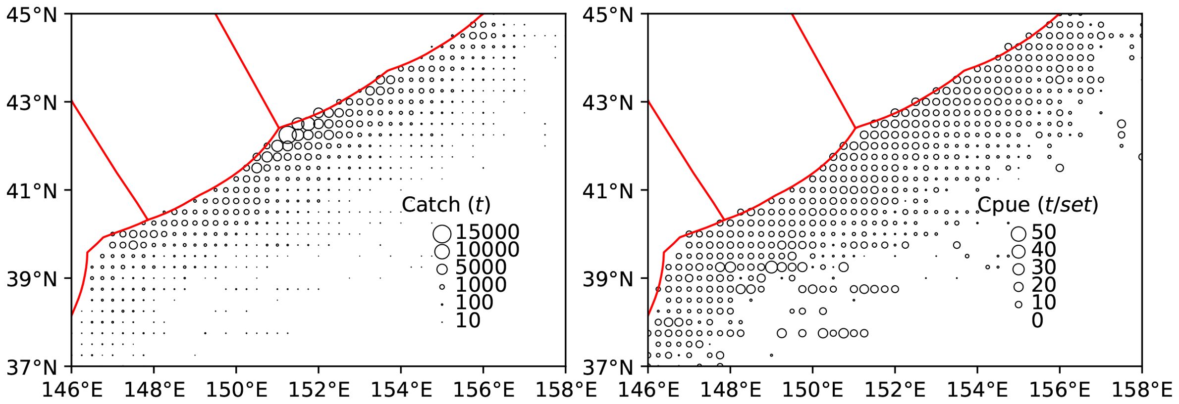
Figure 1. Catch and CPUE distribution of chub mackerel.

Figure 2

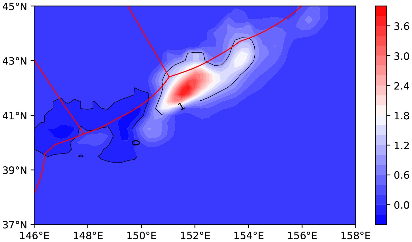
Figure 2. Spatial distribution of coefficients from the geographically weighted regression models for chub mackerel catch and catch per unit effort.

Figure 3

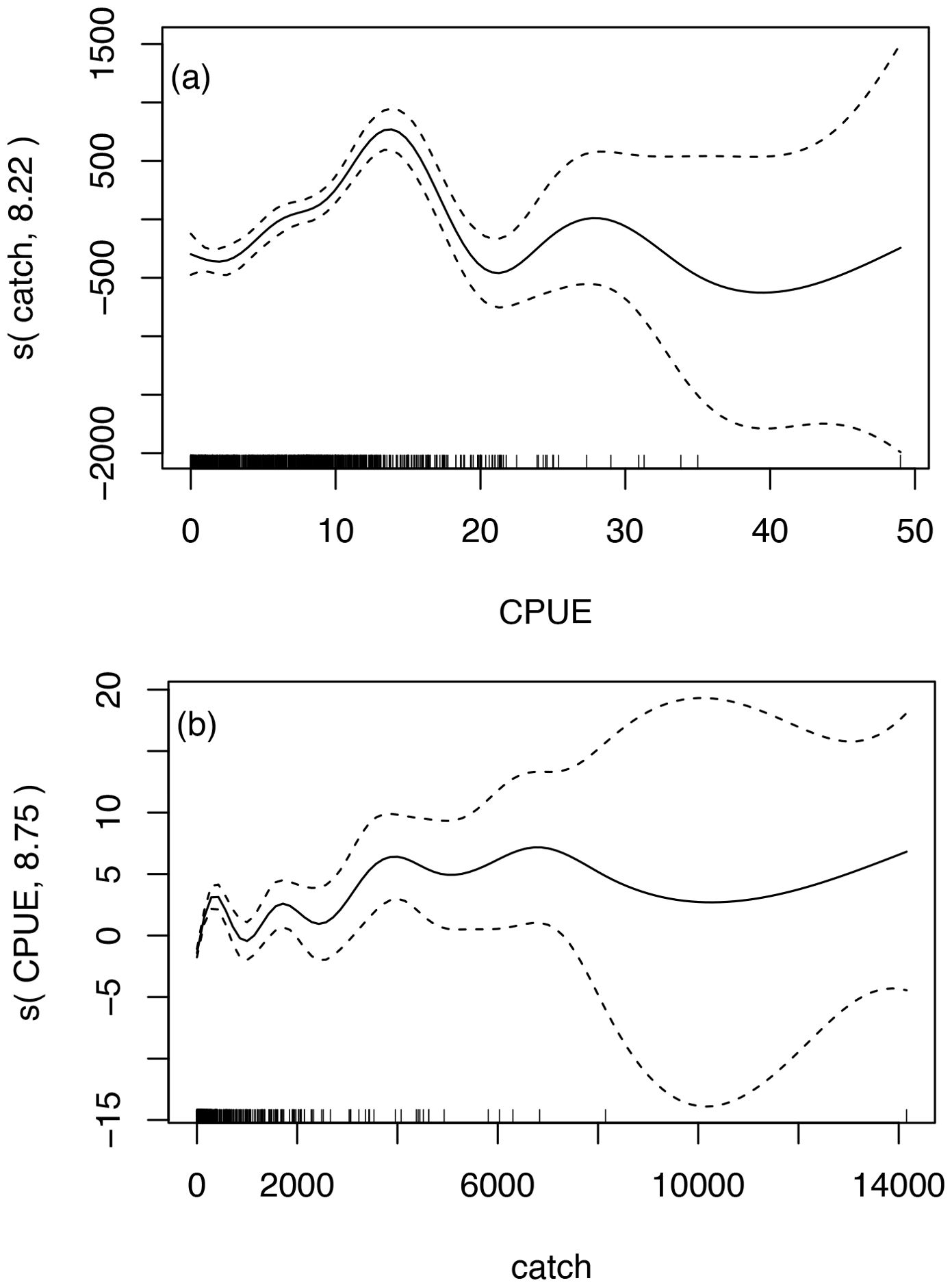
Figure 3. Nonlinear relationships between chub mackerel catch and CPUE in generalized additive models (In (a): Catch yield is the dependent variable, and CPUE is the independent variable; In (b): Catch yield is the independent variable, and CPUE is the dependent variable).

A spatial overlay analysis was conducted between catch yield distributions and the spatial distributions of eddy polarity and mean environmental variables during the fishing days. Fishing locations exhibit a southwest-northeast orientation along Exclusive Economic Zone (EEZ) boundary lines, with higher catch yields observed in proximity to these boundaries (see Figure 4). Spatial analysis of eddy polarity reveals that anticyclonic eddies dominate 57.8% of the grid points (with eddy polarity values >0), indicating a relatively broader distribution of anticyclonic eddies compared to cyclonic eddies within the study area. If fishing locations were randomly distributed in longitude and latitude, catches in areas influenced by anticyclonic eddies would theoretically exceed those in cyclonic eddy-affected regions. Under hypothetical random spatial distribution of catch, anticyclonic eddies account for 10.9% of catches internally and 40.6% externally, while cyclonic eddiesaccount for 10.3% internally and 38.1% externally, suggesting marginally higher catches in anticyclonic eddy-affected regions. However, in the actual observed distribution, chub mackerel catches near anticyclonic eddies are 4.4% internally and 37.8% externally, compared to 15.2% internally and 42.6% externally for cyclonic eddies, demonstrating significantly higher catches near cyclonic eddies. Spatial overlay analysis further shows that high-catch areas predominantly overlap with cyclonic eddy-dominated zones, which form a band along the EEZ boundary (see Figure 4a). Additionally, pronounced frontal zones of SST, Chl-a, and ADT are observed near this cyclonic-eddy-dominated belt (see Figure 4b–d).

Figure 4

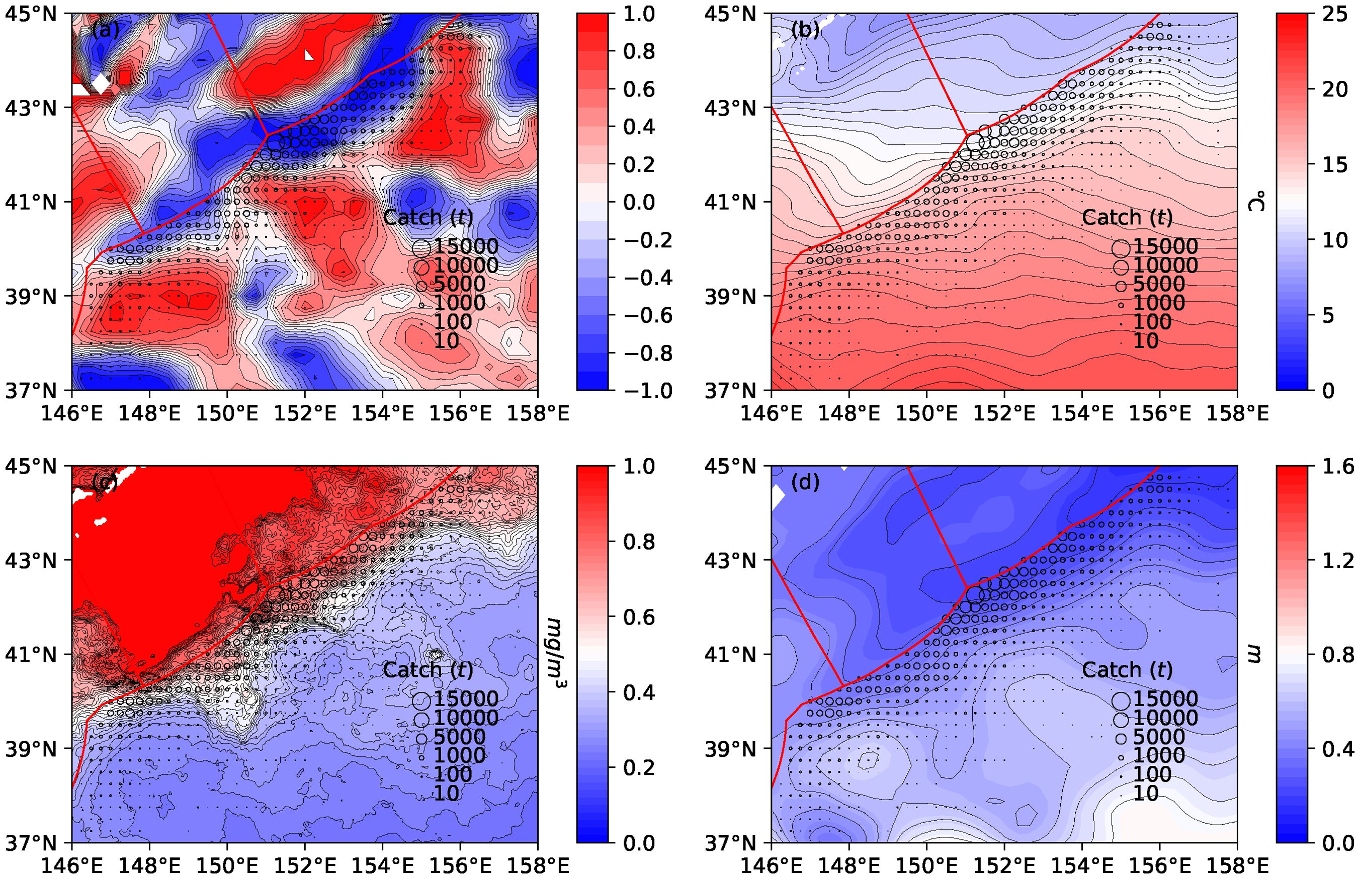
Figure 4. Spatial distributions of catch yields and environmental parameters: (a) Eddy Polarity, (b) Sea Surface Temperature, (c) Chlorophyll-a Concentration, (d) Absolute Dynamic Topography.

Distribution of catch in the normalized eddy-centric coordinate system

The eddy-centric spatial domain was divided into 0.1×0.1 grid cells, with catch statistics calculated for each grid (Figure 5). Under random distribution, catches near anticyclonic and cyclonic eddies are relatively uniform, with slightly higher values near anticyclonic eddies (Figures 5a, b). In observed distributions (Figures 5c, d), catches are sparse inside anticyclonic eddy boundaries, with high-value clusters concentrated outside the boundaries in the northwestern region. In contrast, catches near cyclonic eddies are more abundant, distributed both inside and outside their boundaries, with high-value clusters predominantly in the central-southern zones. Spatial autocorrelation analysis using local Moran’s I for catch distributions in eddy-centric coordinates is shown in Figure 6. For random distributions, aggregation patterns of cyclonic and anticyclonic eddies are similar, exhibiting statistically significant clustering in the 2R region (twice the eddy radius). This likely arises because 66.8% of randomly distributed catch data fall within the 2R zone. However, observed catch distributions show markedly different aggregation patterns compared to random scenarios, with distinct clustering characteristics between cyclonic and anticyclonic eddies.

Figure 5

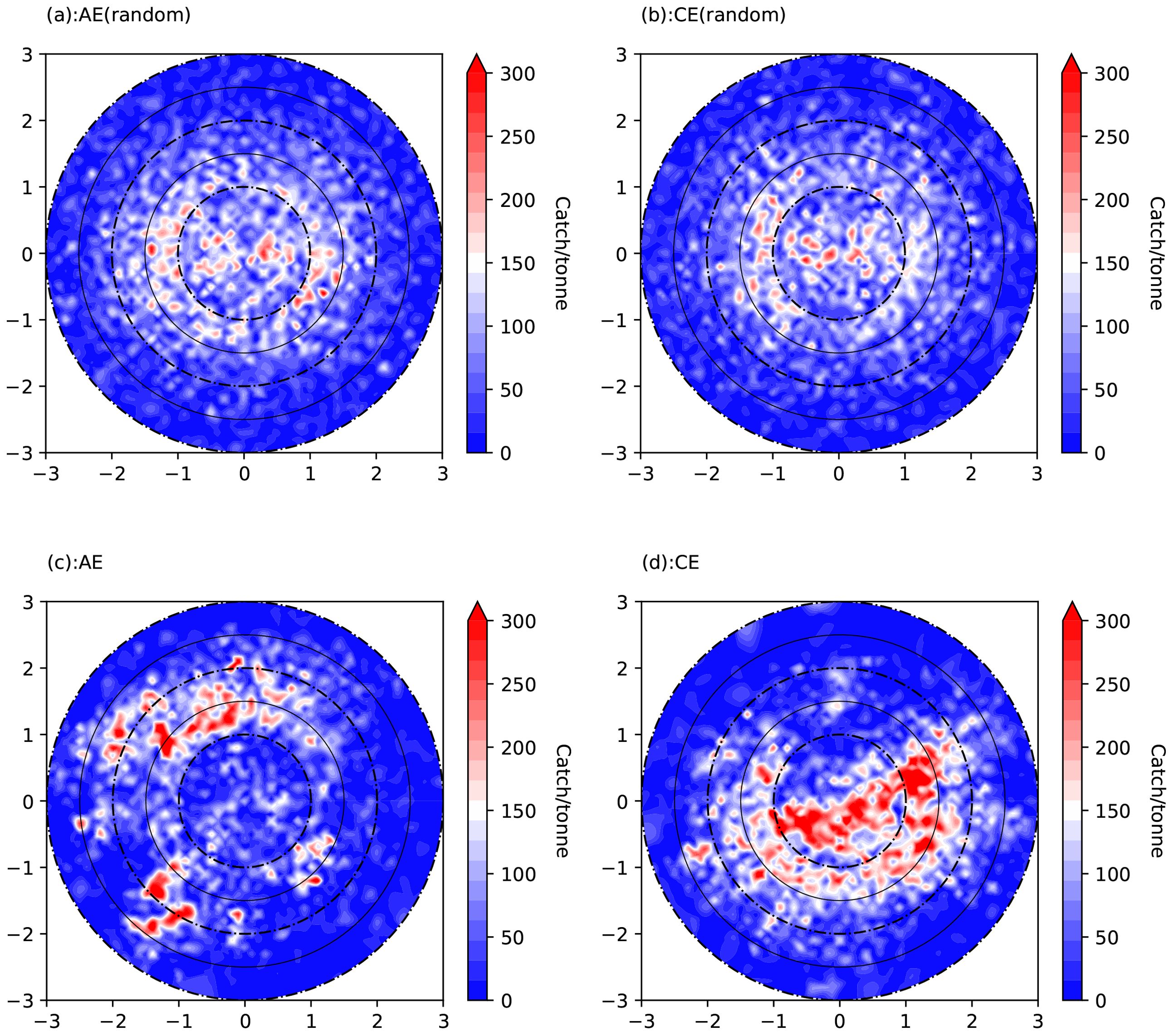
Figure 5. Distribution of catch yield in the normalized eddy coordinate system [(a, b) randomized yield in anticyclonic and cyclonic eddies respectively; (c, d) actual yield in anticyclonic and cyclonic eddies respectively].

Figure 6

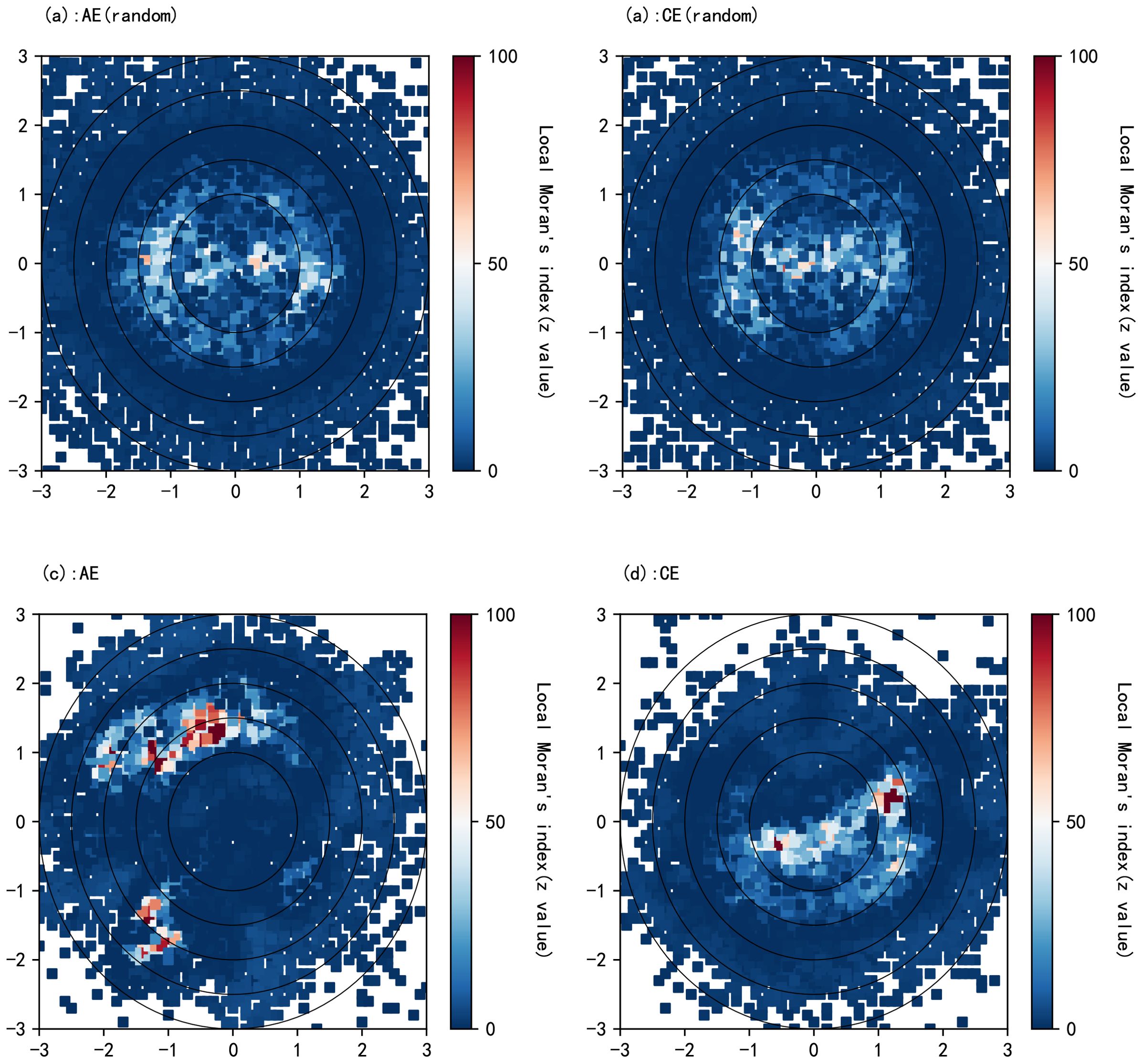
Figure 6. Distribution of local moran’s I for catch yield in the normalized eddy coordinate system [(a, b) represent local moran’s I indices of randomized yields within anticyclonic and cyclonic eddies respectively; (c, d) depict local moran’s I indices of actual yields in anticyclonic and cyclonic eddies correspondingly].

To examine the statistical significance of cyclonic and anticyclonic eddies on the spatial distribution of chub mackerel catch yields, a one-way analysis of variance (ANOVA) was conducted on four datasets: randomized and actual catch distributions within both cyclonic and anticyclonic influenced zones. The four datasets were subjected to Levene’s test for homogeneity of variance, with results indicating non-homogeneous variances across groups (p<0.05). Therefore, the non-parametric Kruskal-Wallis H test was employed to assess intergroup differences. The resulting p-value (<0.01) rejected the null hypothesis, demonstrating statistically significant impacts of cyclonic and anticyclonic eddies on catch yields. Further post-hoc tests using the Games-Howell method were conducted, with results presented in Table 1. The distributions of randomized catch yields between anticyclonic and cyclonic eddy zones failed to exhibit statistically significant differences at the 0.01 significance level. In contrast, significant disparities were observed between actual and randomized catch distributions within both eddy types (p<0.01), as well as between actual catch yields in cyclonic versus anticyclonic eddy-influenced regions (p<0.01). These results conclusively demonstrate that mesoscale eddies exert statistically significant impacts on catch distribution patterns, with distinct ecological effects between cyclonic and anticyclonic eddies.

Table 1

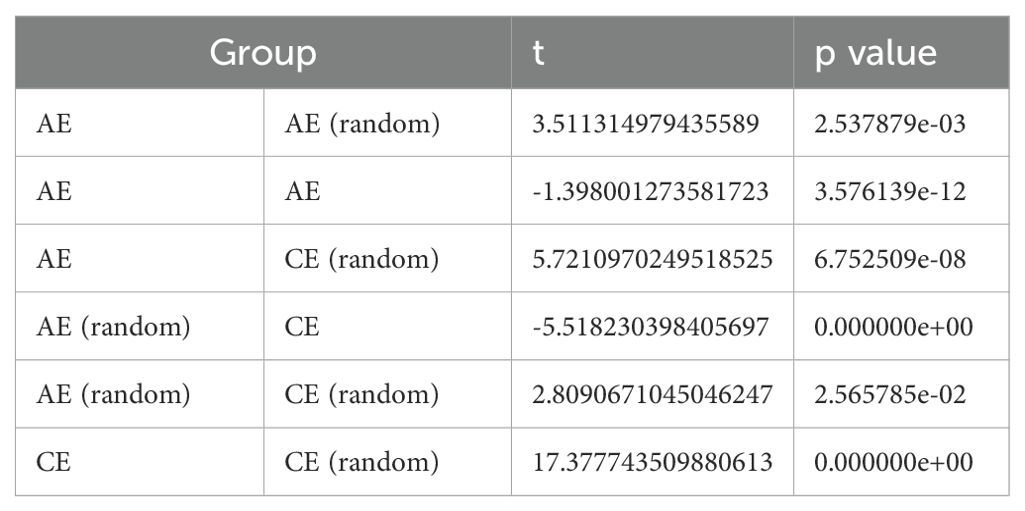
Table 1. Results of the Games-Howell post hoc test for four groups of catch yield in the normalized eddy coordinate system.

The statistical results of catch yield along the radius with a bin width of 0.05 in the Normalized Eddy Coordinate System are shown in Figure 7. In the random distribution, the radial patterns of catch yield in cyclonic and anticyclonic eddy-affected zones are relatively similar, with slightly higher yields in anticyclonic eddy-affected zones. This aligns with the observation that anticyclonic eddies occupy a slightly larger area within the study region compared to cyclonic eddies. In stark contrast, actual catch distributions reveal inverse trends: within 1.5R (R = eddy radius), of eddy centers, cyclonic-eddy zones demonstrate significantly higher yields than both anticyclonic-eddy areas (p<0.01) and randomized baselines, while anticyclonic-eddy catches remain lower than both cyclonic-eddy yields and random distributions. These disparities diminish substantially beyond 1.5R (Figure 7). The Kolmogorov–Smirnov test revealed statistically significant differences (p< 0.01) between the distribution curves of yield along the radii of cyclonic and anticyclonic eddies within the 1.5R zone (relative to the eddy core). Cumulative distribution analysis (Figure 8) further demonstrates that cyclonic-eddy catches consistently surpass both anticyclonic-eddy and randomized distributions across all radial distances, whereas anticyclonic-eddy yields only exceed random baselines beyond 2R.

Figure 7

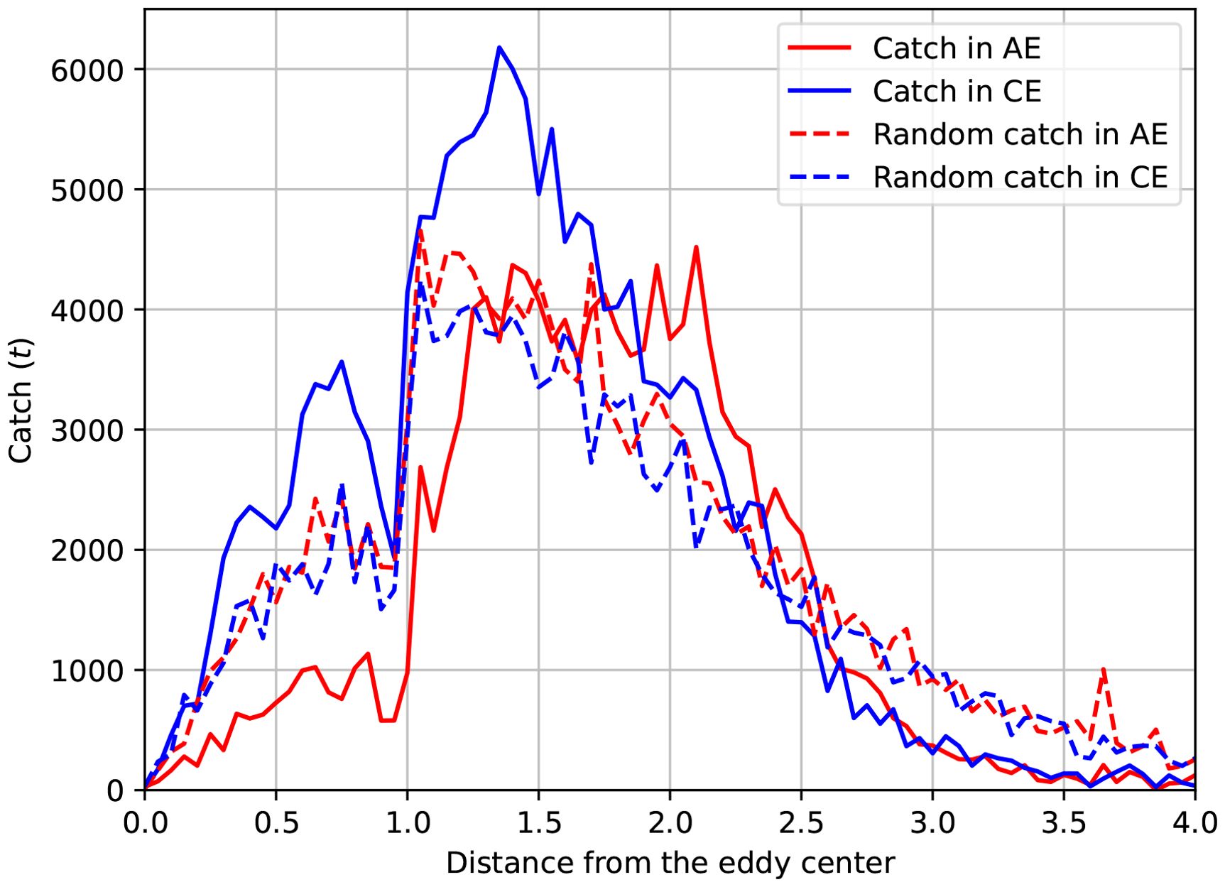
Figure 7. Radial distribution of catch yield in the normalized eddy coordinate system.

Figure 8

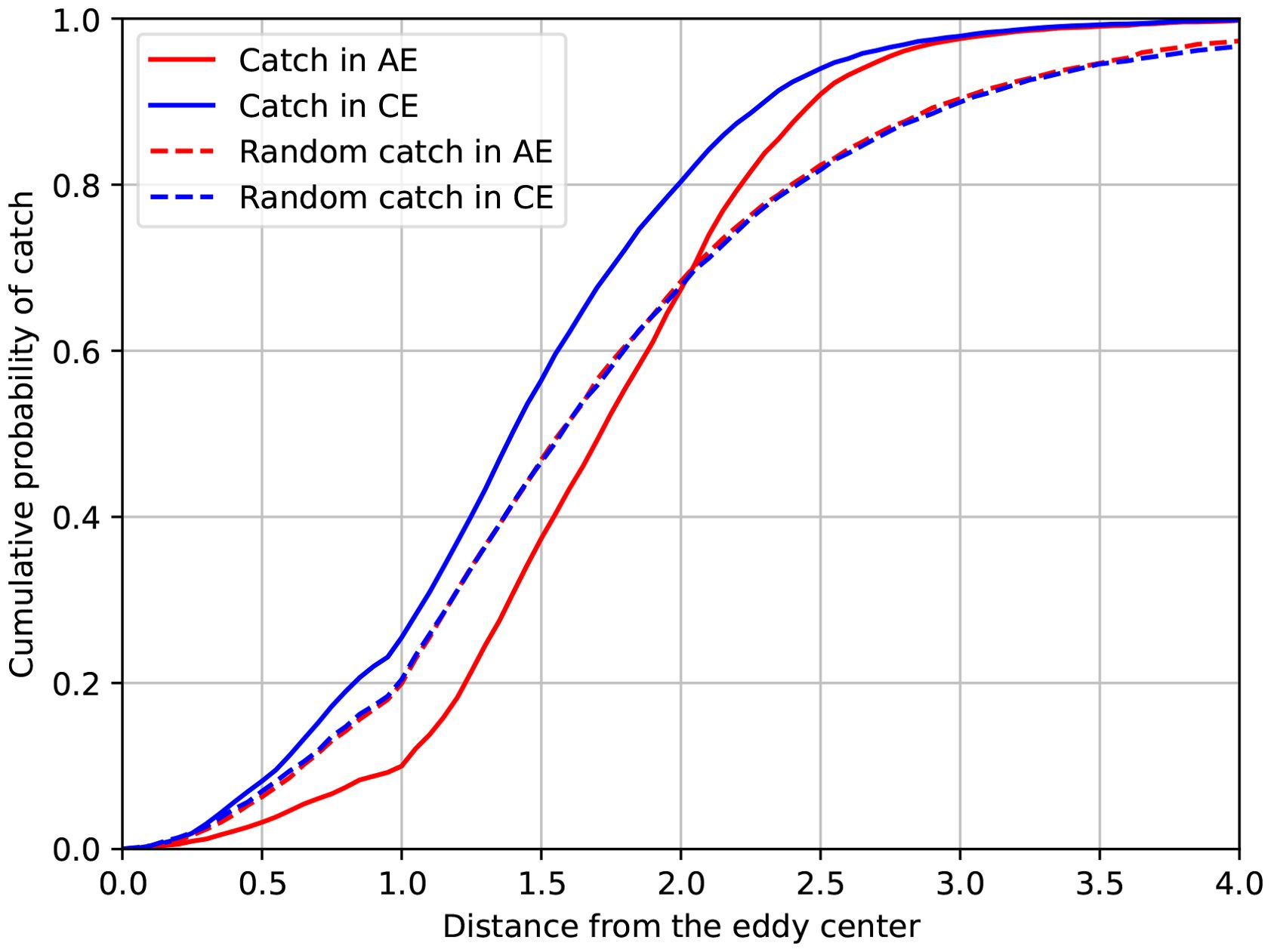
Figure 8. Cumulative radial distribution of catch yield in the normalized eddy coordinate system.

Catch hotspots in mesoscale eddy interaction zones

Hotspots of catch yield (Z > 2.58, p< 0.01) in the normalized eddy coordinate system correspond to high-yield aggregation zones of chub mackerel. As shown in Figure 9, the hotspots of both randomized and actual catch yields outside the eddy boundary lines exhibit more extensive spatial distribution in AC and CA eddy configurations compared to AA and CC types. The proportion of randomized catch yield in eddy interaction zones AC&CA reaches 50.44% compared to 28.31% in AA & CC configurations, with corresponding actual yield proportions measuring 52.95% and 27.52% respectively. Interaction zones between different eddy types demonstrate approximately twice the yield of homogeneous eddy configurations. Although both random and actual catch hotspots exhibit broader spatial coverage in AC and CA regions compared to AA and CC, their distribution patterns demonstrate distinct characteristics. In the first-nearest eddy space, hotspots predominantly form ring-shaped patterns between 1R and 2R from the eddy center with spatial configurations exhibiting high similarity across all four scenarios (AC-1, CA-1, AA-1, CC-1). Hotspots predominantly exhibit fragmented dispersion patterns beyond 2R, characterized by discontinuous clusters with reduced spatial coherence across all scenarios. For actual catch hotspots, in AA-1 space, aggregations predominantly cluster along the left flank of anticyclonic eddies, in CC-1 space, Hotspots concentrate within the mid-lower sections of cyclonic eddies, in AA-2/CC-2 spaces, catch distributions exhibit scattered dispersion patterns with reduced spatial coherence. In AC/CA Scenarios, actual catch hotspots primarily clustered in the northwest quadrant of anticyclonic eddies, concentrated in mid-lower sectors of cyclonic eddies. This spatial pattern aligns with Figure 4a, where catches predominantly distribute along a southwest-northeast oriented frontal zone dominated by adjacent cyclonic-anticyclonic eddy pairs (with cyclonic eddies positioned northwest of anticyclonic eddies), exhibiting consistent lateral bias toward the cycloniceddy sector. In the hotspot areas of randomly distributed catches, the actual spatial area represented by individual grid cells is larger than in non-hotspot regions, leading to high-value aggregation of random catches within these cells. In contrast, the hotspot areas of actual catch distributions reflect more suitable habitats actively selected by Chub mackerel, which consequently exhibit high catch values within these grids. The distinct hotspot distribution characteristics between random and actual catches in mesoscale eddy interaction zones demonstrate the significant influence of eddies on fishing ground distributions.

Figure 9

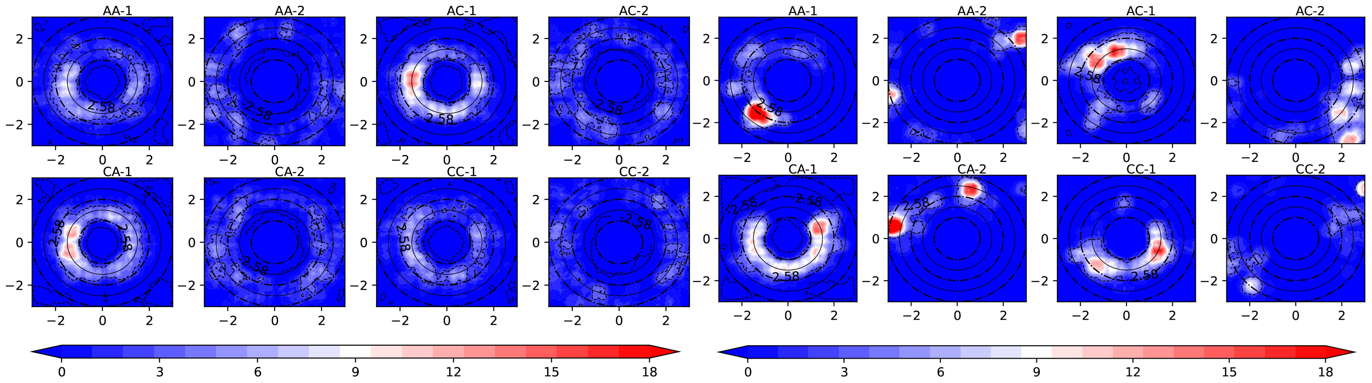
Figure 9. Hotspot distribution of chub mackerel yield in eddy interaction zones (AC denotes that the two eddies closest to the fishing site are an anticyclonic eddy followed by a cyclonic eddy, indicating the fishing site is within the interaction zone of an anticyclonic and cyclonic eddy pair. AC-1 refers to the nearest anticyclonic eddy in the AC pair, while AC-2 represents the second-nearest anticyclonic eddy. Definitions for CA, AA, and CC follow analogous logic. The contours in the figure mark the absolute Z-values of the local Getis-Ord index equal to 2.58.).

Spatial distribution of environmental variables in a normalized eddy coordinate system

To investigate the mechanisms driving the distribution patterns of fishery catches in mesoscale eddy regions, this study identified the nearest eddies associated with over 30,000 fishing locations. By integrating SST, Chl-a, and ADT data, we extracted environmental variables within a 3R radius (three times the eddy core radius) from eddy centers and visualized their mean values in the normalized eddy coordinate system (see Figure 10). The distribution of oceanic environmental parameters within cyclonicand anticyclonic eddies exhibits distinct differences. Anticyclonic eddies are characterized by higher SST, lower Chl-a, and elevated ADT, whereas cyclonic eddies show lower SST, higher Chl-a, and depressed ADT. Mesoscale eddy boundary regions are characterized by pronounced environmental frontal zones that circumnavigate the eddy core, exhibiting distinct banded distribution patterns. Frontal zones exhibit intense variations in environmental parameters, characterized by sharp horizontal gradients across key variables. Cyclonicand anticyclonic eddies exhibit distinct frontal configurations, with thermal fronts, ADT fronts, and Chl-a fronts primarily located along the northern flank of anticyclonic eddies and the southern periphery of cyclonic eddies.

Figure 10

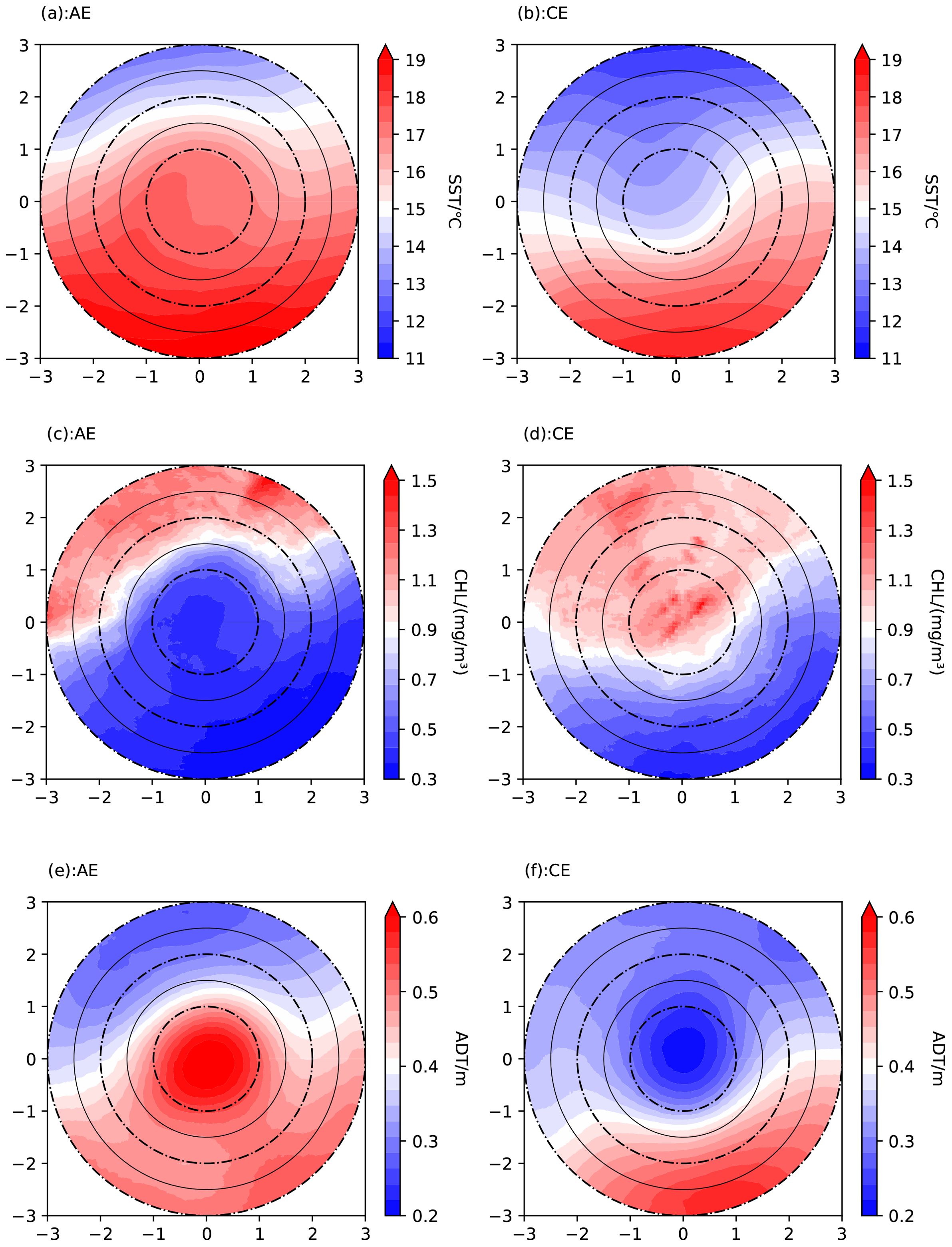
Figure 10. Distribution of environmental variables in the normalized eddy coordinate system (Subplots (a), (c), and (e) show the distributions of SST, CHL-a, and ADT in the normalized coordinate system for AEs, respectively; Subplots (b), (d), and (f) show the distributions of SST, CHL-a, and ADT in the normalized coordinate system for CEs).

GAM model fitting results

GAM models were applied to investigate the relationships between fishery yield and environmental variables within the standardized eddy coordinate system for both cyclonic and anticyclonic eddies. The variance explained by the models reached 47.2% for cyclonic eddies and 32.8% for anticyclonic eddies, with all variables demonstrating statistically significant effects (p< 0.05). These results indicate that environmental factors significantly influence the spatial distribution of yields in both eddy types. Notably, the distribution of yields within the eddy framework exhibited strong correlations with SST, Chl-a, and ADT.

Based on the GAM fitting results (see Figure 11), the spatial distribution of catch within cyclonic eddies exhibits near-bilateral symmetry, with a balanced east-west centroid distribution and a slight southward shift along the meridional axis, consistent with the catch aggregation patterns in cyclonic eddies shown in Figures 5c, 6c. In contrast, catch distribution in anticyclonic eddies lacks symmetrical characteristics, with the centroid skewed toward the western and northern sectors of the eddies, which aligns with the distribution characteristics of cyclonic-eddy catch aggregation depicted in Figures 5d, 6d High-density catch areas are associated with Chl-a of 0.2 – 2 mg/m³, SST ranges of 10 – 20°C, and ADT values of 0.3 – 0.6 m.

Figure 11

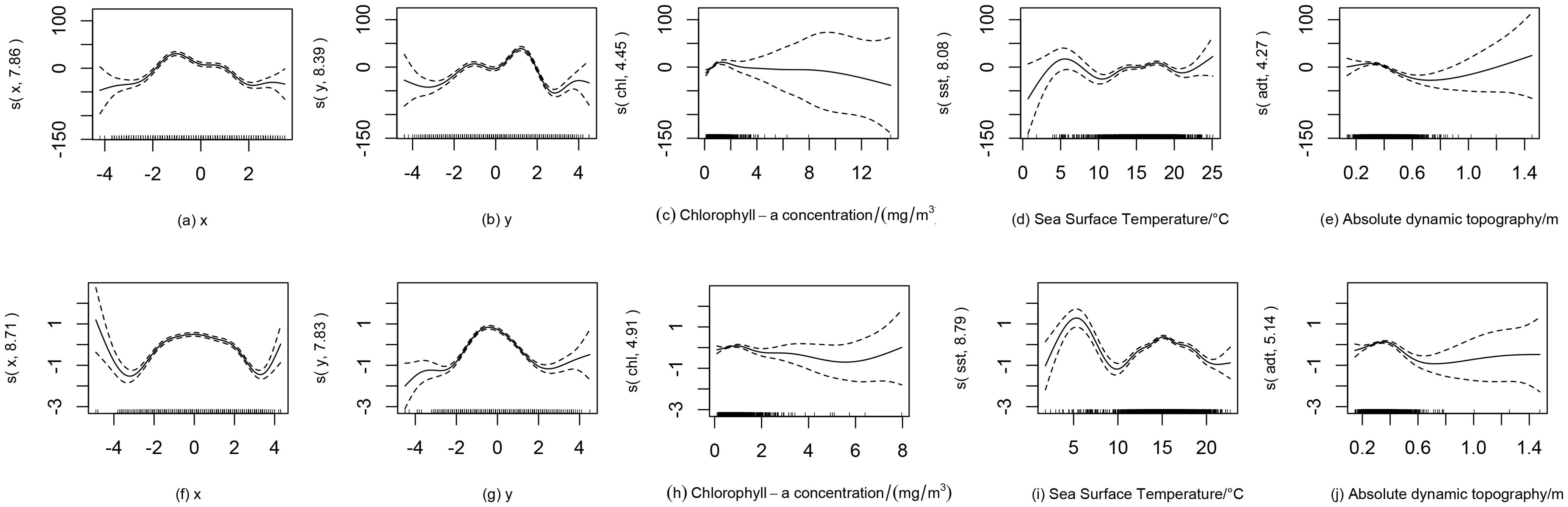
Figure 11. The relationship between variables and fitted smooth terms [dashed lines indicate 95% confidence intervals of the smoothed curves. (a–e) correspond to anticyclonic eddies, while (f–j) are associated with cycloniceddies].

Discussion

This study analyzes the spatial distributions of eddy polarity and mean values of SST, Chl-a, and ADT over 1,228 accumulated fishing days during chub mackerel operations from 2018 to 2022. During fishing operations, a southwest-northeast trending low eddy polarity zone (cyclonic-eddy dominant region) was identified along the outer boundary of Japan’s Exclusive Economic Zone in the Northwest Pacific Ocean. This characteristic spatial pattern of eddy polarity was not evident during other temporal periods (Cui et al., 2017). Within and along the northwestern flank of this cyclonic-eddy-dominated belt, elevated Chl-a and depressed sea surface temperatures were observed, while the southeastern sector exhibited diminished Chl-a levels and warmer SST values. This spatial pattern suggests that the southwest-northeast-oriented eddy belt potentially inhibits southeastward transport of chlorophyll-rich waters and cooler water masses, serving as a dynamic barrier to cross-frontal biogeochemical exchange. Cyclonic eddies and anticyclonic eddies exhibit markedly different distribution patterns of oceanographic parameters (Sun et al., 2017), resulting in pronounced variations in these variables within their interaction zones. Figure 4a overlaying eddy polarity and chub mackerel catch data clearly demonstrates concentrated yields in cyclonic-eddy-dominated sectors and interfacial zones between cyclonic and anticyclonic eddies. In the randomized catch distribution, 50.44% occurred in transitional zones between cyclonic and anticyclonic eddies, while AA and CC interfaces accounted for 28.31%, indicating greater spatial coverage in cyclonic- anticyclonic transitional areas. Correspondingly, the actual catch distribution showed 52.95% in cyclonic- anticyclonic zones and 27.52% in AA and CC regions. Both actual and randomized catch distributions exhibit higher yields in cyclonic- anticyclonic transition zones. However, Figure 9 (Hotspot distribution of chub mackerel yield in eddy interaction zones) reveals fundamentally distinct spatial clustering for actual yields within these transitional areas compared to random patterns. This demonstrates that high productivity in cyclonic- anticyclonic interfaces is non-random and not solely driven by larger spatial extent. Oceanographically, these zones coincide with the Kuroshio-Oyashio Confluence Front (Xing et al., 2023b; 2024a), where intensified frontal processes synergize with mesoscale eddy interactions to enhance productivity. This aligns with established biophysical principles: oceanic frontal regions with sharp environmental gradients often form optimal fishing grounds due to nutrient enrichment and prey concentration (Bakun, 2006). The cyclonic and anticyclonic eddies closest to the fishing locations exhibit distinct distribution patterns: anticyclonic eddies are predominantly located southeast of cyclonic eddies, while cyclonic eddies concentrate northwest of anticycloniceddies. This spatial pattern aligns with the distribution observed in Figure 4a, where elevated catch yields are concentrated within a southwest-northeast trending band straddling the boundary between cyclonic eddy-dominant and anticyclonic eddy-dominant regions.

Projecting both randomized and actual chub mackerel catch data onto standardized eddy-centric coordinate systems for anticyclonic and cyclonic eddies reveals significant distributional divergences between the two regimes. The random catch yields are predominantly distributed within the 2R from eddy centers, indicating that spatial grid points projected onto the eddy-centric coordinate system mainly fall within this area. Furthermore, the distribution of random yields exhibits greater dispersion and uniformity in both cyclonic and anticyclonic eddies. If the influence of eddies on yield distribution is disregarded, the spatial characteristics of yields in anticyclonic and cyclonic eddy environments would exhibit similar distribution patterns. Actual catch yields are predominantly concentrated in the northwest quadrant between R and 2.5R from anticyclonic eddy centers, while distributed within the 2R of cyclonic eddies with higher density in the southeastern sector and relatively sparse in the northwestern sector. Statistical analysis of Moran’s I index confirmed the spatial heterogeneity of these distribution patterns is statistically significant. Quantitative assessments revealed 57.8% of total yields occurred near cyclonic eddies versus 42.2% near anticyclonic eddies, contrasting with their respective random distribution proportions of 51.5% and 48.5%. Kolmogorov-Smirnov tests demonstrated significant differences (p<0.01) in yield distribution patterns along the radial gradients of cyclonic versus anticyclonic eddies. These findings collectively demonstrate that fishing grounds are predominantly displaced from anticyclonic eddies, with primary aggregation along their northwestern outer margins, while exhibiting closer proximity to cyclonic eddies where distributions are concentrated in southeastern sectors. This is consistent with the 2021 – 2023 June-August offshore comprehensive survey showing that marine organisms in the Kuroshio-Oyashio confluence zone are mainly distributed in the northern areas of anticyclonic eddies and southern areas of cyclonic eddies (Su et al., 2025). Studies indicate that Japanese flying squid (Todarodes pacificus) are more abundant in anticyclonic eddies during years of the Kuroshio Current’s large meander (LM) path (Zhang et al., 2022), which may be attributed to the increased generation of anticyclonic eddies in the northern Kuroshio Extension region during LM years (Zhang et al., 2025). The warm water and highly oxygenated water within anticyclonic eddies allow large pelagic fish such as tuna and sharks to forage in deeper zones and prolong their residence time within these eddies (Braun et al., 2019; Durán Gómez et al., 2020; Lindo-Atichati et al., 2012). These findings demonstrate varying dependencies of different fish species on environmental factors. In contrast, this study reveals that chub mackerel tend to aggregate near cyclonic eddies while avoiding anticyclonic eddies, exhibiting a distinct spatial preference compared to large tuna species predominantly found in anticyclonic eddies.

Numerous studies have demonstrated that key environmental factors influencing the spatial distribution of chub mackerel fishing grounds include SST, Chl-a, and ADT (Fan et al., 2020; Li et al., 2025, 2024). Within mesoscale eddies, Chl-a displays a northwest-high to southeast-low gradient, while SST and ADT exhibit an inverse spatial pattern (northwest-low to southeast-high). These distribution trends are consistent with the regional characteristics of the Northwestern Pacific Ocean for these environmental variables (Xing et al., 2023a; Fan et al., 2019). This region is situated within the confluence zone of the Kuroshio and Oyashio Currents, exhibiting pronounced oceanographic frontal gradients (Xing et al., 2023b; 2024a). Analysis of fishery-linked oceanographic elements within mesoscale eddies reveals a distinct southwest-northeast oriented front. This frontal zone exhibits contrasting oceanographic conditions: the northwestern sector features lower SST, higher Chl-a, and lower ADT, while the southeastern sector displays higher SST, lower Chl-a, and elevated ADT. The positioning of environmental fronts—whether in the northwestern or southeastern sector of mesoscale eddies—is determined by integrating background fields of oceanographic parameters with eddy-scale localized patterns. For anticyclonic eddies, high SST in the central core converges with colder northwestern waters, establishing thermal fronts predominantly in the northwestern sector. Mirroring this mechanism, cyclonic eddies exhibit low central SST interacting with warmer southeastern waters, forming thermal fronts primarily in the southeastern sector. Similarly, the fronts associated with ADT and Chl-a can be explained by analogous mechanisms, with their frontal zones positioned in the northwestern part of anticyclonic eddies and the southeastern part of cyclonic eddies.This suggests that the spatial distribution patterns of environmental parameters within mesoscale eddies are not only dependent on their radial distance from the eddy center but also influenced by the regional-scale background distribution of these parameters in the surrounding ocean. The distribution of parameters within eddy-influenced regions will affect the distribution of biological resources. Arur et al. (2014; 2020) demonstrated through their study of coastal mesoscale eddies and commercial fishing catch data in the Indian Ocean that distinct sub-regions within eddy systems are associated with specific fishing strategies and species compositions, though the causal mechanisms remain unexamined. In the eddies associated with fishing locations in this study, frontal zones of SST, Chl-a, and ADT were predominantly located in the northern sectors of anticyclonic eddies and southern sectors of cyclonic eddies, mirroring the spatial distribution patterns of catch hotspots within eddy systems. Furthermore, Generalized Additive Models applied to the standardized eddy coordinate system demonstrated high explanatory power in resolving nonlinear relationships between environmental parameters and catch yields. This statistically significant correlation (p<0.05) confirms that the spatial distribution of catches within the standardized eddy framework is mechanistically linked to the environmental parameters SST, ADT and Chl-a. Notably, elevated Chl-a near cyclonic eddies—a key bioenergetic feature—may partially explain their enhanced ecological suitability as habitats for chub mackerel compared to anticyclonic eddies.

Data availability statement

Publicly available datasets were analyzed in this study. This data can be found here: http://marine.copernicus.eu/services-portfolio/access-to-products/ and https://www.aviso.altimetry.fr/en/data/products/value-added-products/global-mesoscale-eddy-trajectory-product.html.

Author contributions

XF: Writing – original draft, Software, Conceptualization, Writing – review & editing. XC: Writing – review & editing. SY: Writing – review & editing. FT: Resources, Writing – review & editing.

Funding

The author(s) declare financial support was received for the research and/or publication of this article. This study was supported by the National Key R&D Program of China (2023YFD2401305).

Acknowledgments

We express profound gratitude to the Copernicus Marine Environment Monitoring Service (CMEMS) and AVISO (Archiving, Validation and Interpretation of Satellite Oceanographic Data) for data provision, and sincerely appreciate peer reviewers for their constructive suggestions and expert comments.

Conflict of interest

The authors declare that the research was conducted in the absence of any commercial or financial relationships that could be constructed as a potential conflict of interest.

The reviewer DX declared a past co-authorship with the author SY to the handling editor at the time of review.

Generative AI statement

The author(s) declare that no Generative AI was used in the creation of this manuscript.

Any alternative text (alt text) provided alongside figures in this article has been generated by Frontiers with the support of artificial intelligence and reasonable efforts have been made to ensure accuracy, including review by the authors wherever possible. If you identify any issues, please contact us.

Publisher’s note

All claims expressed in this article are solely those of the authors and do not necessarily represent those of their affiliated organizations, or those of the publisher, the editors and the reviewers. Any product that may be evaluated in this article, or claim that may be made by its manufacturer, is not guaranteed or endorsed by the publisher.

References

Arur A., Krishnan P., George G., Goutham Bharathi M. P., Kaliyamoorthy M., Hareef Baba Shaeb K., et al. (2014). The influence of mesoscale eddies on a commercial fishery in the coastal waters of the Andaman and Nicobar Islands, India. Int. J. Remote Sens. 35, 6418–6443. doi: 10.1080/01431161.2014.958246

Crossref Full Text | Google Scholar

Arur A., Krishnan P., Kiruba-Sankar R., Suryavanshi A., Lohith Kumar K., Kantharajan G., et al. (2020). Feasibility of targeted fishing in mesoscale oceanic eddies: a study from commercial fishing grounds of Andaman and Nicobar Islands, India. Int. J. Remote Sens. 415011–5045. doi: 10.1080/01431161.2020.1724347

Crossref Full Text | Google Scholar

Bakun A. (2006). Fronts and eddies as key structures in the habitat of marine fish larvae: opportunity, adaptive response and competitive advantage. Sci. Mar. 70(S2), 105–122. doi: 10.3989/scimar.2006.70s2105

Crossref Full Text | Google Scholar

Braun C. D., Gaube P., Sinclair-Taylor T. H., et al. (2019). Mesoscale eddies release pelagic sharks from thermal constraints to foraging in the ocean twilight zone. PNAS 116, 17187–17192. doi: 10.1073/pnas.1903067116

PubMed Abstract | Crossref Full Text | Google Scholar

Chelton D. B., Schlax M. G., and Samelson R. M. (2011). Global observations of nonlinear mesoscale eddies. Prog. Oceanogr. 91, 167–216. doi: 10.1016/j.pocean.2011.01.002

Crossref Full Text | Google Scholar

Chelton D. B., Schlax M. G., Samelson R. M., et al. (2007). Global observations of large oceanic eddies. Geophys. Res. Lett. 34, L15606. doi: 10.1029/2007GL030812

Crossref Full Text | Google Scholar

Cui W., Wang W., Ma Y., et al. (2017). Identification and analysis of mesoscale eddies in the northwestern pacific ocean from 1993 – 2014 based on altimetry data. Haiyang Xuebao 39, 16–28. doi: 10.3969/j.issn.0253-4193.2017.02.002

Crossref Full Text | Google Scholar

Dong C. M., McWilliams J. C., Liu Y., et al. (2014). Global heat and salt transports by eddy movement. Nat. Commun. 5, 3294. doi: 10.1038/ncomms4294

PubMed Abstract | Crossref Full Text | Google Scholar

Durán Gómez G. S., Nagai T., and Yokawa K. (2020). Mesoscale warm-core eddies drive interannual modulations of swordfish catch in the kuroshio extension system. Front. Mar. Sci. 7. doi: 10.3389/fmars.2020.00680

Crossref Full Text | Google Scholar

Fan X. M., Fan W., Yang S. L., et al. (2019). A new reconstruction method for the 3-D temperature field in the western pacific ocean based on steric height and SST. Period. Ocean Univ. China. 49 (12), 1–10. doi: 10.16441/j.cnki.hdxb.20180357

Crossref Full Text | Google Scholar

Fan X. M., Tang F. H., Cui X. S., et al. (2020). Habitat suitability index for chub mackerel (Scomber japonicus) in the Northwest Pacific Ocean. Haiyang Xuebao 42, 34–43. doi: 10.3969/j.issn.0253–4193.2020.12.004

Crossref Full Text | Google Scholar

Hu Z. F., Tan Y. H., Song X. Y., Zhou L. B., Lian X. P., Huang L. M., et al. (2014). Influence of mesoscale eddies on primary production in the South China Sea during spring inter-monsoon period, Acta Oceanol. Sin. 33, 118–128. doi: 10.1007/s13131-014-0431-8

Crossref Full Text | Google Scholar

Li J. S., Cui X. S., Tang F. H., et al. (2024). Spatiotemporal analysis of marine environmental influence on the distribution of chub mackerel in the Northwest Pacific Ocean based on geographical and temporal weighted regression. J. Sea Res. 200, 102514. doi: 10.1016/j.seares.2024.102514

Crossref Full Text | Google Scholar

Li J. S., Zhou W. F., Dai Y., Tang F. H., Wu Y. M., Zhang H., et al. (2025). Effects of western boundary currents and sea surface temperature anomalies on interannual variability of chub mackerel abundance in the Northwest Pacific. J. Sea Res. 203, 102561. doi: 10.1016/j.seares.2024.102561

Crossref Full Text | Google Scholar

Lindo-Atichati D., Bringas F., Goni G., et al. (2012). Varying mesoscale structures influence larval fish distribution in the northern Gulf of Mexico. Mar. Ecol. Prog. Ser. 463, 245–257. doi: 10.3354/meps09860

Crossref Full Text | Google Scholar

Mahadevan A., D’Asaro E., Lee C., et al. (2012). Eddy-driven stratification initiates north atlantic spring phytoplankton blooms. Science 337, 54–58. doi: 10.1126/science.1218740

PubMed Abstract | Crossref Full Text | Google Scholar

McGillicuddy D. J. Jr. (2016). Mechanisms of physical-biological-biogeochemical interaction at the oceanic mesoscale. Ann. Rev. Mar. Sci. 8, 125–159. doi: 10.1146/annurev-marine-010814-015606

PubMed Abstract | Crossref Full Text | Google Scholar

Shiraishi T., Okamoto K., Yoneda M., Sakai T., Ohshimo S., Onoe S., et al. (2008). Age validation, growth and annual reproductive cycle of chub mackerelScomber japonicusoff the waters of northern Kyushu and in the East China Sea. Fish. Sci. 74, 947–954. doi: 10.1111/j.1444-2906.2008.01612.x

Crossref Full Text | Google Scholar

Su R. S., Wei Y. L., Tang Z. Y., et al. (2025). Effects of eddies on catch in mid-pelagic species in the Kuroshio-Oyashio confluence region. J. Shanghai Ocean Univ. 34, 382–393. doi: 10.12024/jsou.20240404524

Crossref Full Text | Google Scholar

Sun W. J., Dong C. M., Tan W., et al. (2018). Vertical structure anomalies of oceanic eddies and eddy-induced transports in the south China sea. Remote Sens. 10, 795. doi: 10.3390/rs10050795

Crossref Full Text | Google Scholar

Sun W. J., Dong C. M., Wang R. Y., et al. (2017). Vertical structure anomalies of oceanic eddies in the Kuroshio Extension region. J. Geophys. Res. Oceans 122, 1476–1496. doi: 10.1002/2016JC012226

Crossref Full Text | Google Scholar

Tang F. H., Dai S. W., Fan W., et al. (2020). Study on stomach composition and feeding level of chub mackerel in the Northwest Pacific. J. Agric. Sci. Technol. 22, 138–148. doi: 10.13304/j.nykjdb.2019.0210

Crossref Full Text | Google Scholar

Wang L. M., Ma S. Y., Liu Y., Li J. C., Liu S. G., Lin L. S., et al. (2021). Fluctuations in the abundance of chub mackerel in relation to climatic/oceanic regime shifts in the northwest Pacific Ocean since the 1970s. J. Mar. Syst. 218, 103541. doi: 10.1016/j.jmarsys.2021.103541

Crossref Full Text | Google Scholar

Watanabe C. and Yatsu A. (2006). Long-term changes in maturity at age of chub mackerel (Scomber japonicus) in relation to population declines in the waters off northeastern Japan. Fish. Res. 78, 323–332. doi: 10.1016/j.fishres.2006.01.001

Crossref Full Text | Google Scholar

Xing Q. W., Yu H. Q., and Wang H. (2024a). Global mapping and evolution of persistent fronts in Large Marine Ecosystems over the past 40 years. Nat. Commun. 15, 4090. doi: 10.1038/s41467-024-48566-w

PubMed Abstract | Crossref Full Text | Google Scholar

Xing Q. W., Yu H. Q., and Wang H. (2024b). Mesoscale eddies exert inverse latitudinal effects on global industrial squid fisheries. Sci. Total Environ. 960, 175211. doi: 10.1016/j.scitotenv.2024.175211

PubMed Abstract | Crossref Full Text | Google Scholar

Xing Q. W., Yu H. Q., Wang H., et al. (2023a). Mesoscale eddies modulate the dynamics of human fishing activities in the global midlatitude ocean. Fish Fish. 24, 527–543. doi: 10.1111/faf.12742

Crossref Full Text | Google Scholar

Xing Q. W., Yu H. Q., Wang H., et al. (2023b). A sliding-window-threshold algorithm for identifying global mesoscale ocean fronts from satellite observations. Prog. Oceanogr. 216, 103072. doi: 10.1016/j.pocean.2023.103072

Crossref Full Text | Google Scholar

Xu G. J., Dong C. M., Liu Y., et al. (2019). Chlorophyll rings around ocean eddies in the north pacific. Sci. Rep. 9. doi: 10.1038/s41598-018-38457-8

PubMed Abstract | Crossref Full Text | Google Scholar

Yu W., Guo A., Zhang Y., et al. (2018). Climate-induced habitat suitability variations of chub mackerel Scomber japonicus in the East China Sea. Fish. Res. 207, 63–73. doi: 10.1016/j.fishres.2018.06.007

Crossref Full Text | Google Scholar

Yu W., Jian W., Chen X. J., et al. (2021). Effects of climate variability on habitat range and distribution of chub mackerel in theEast China sea. J. Ocean Univ. China 20, 1483–1494. doi: 10.1007/s11802-021-4760-x

Crossref Full Text | Google Scholar

Zhang C. C., Yang Y. X., and Wang F. M. (2013). Spatial-Temporal features of eddies in the North Pacific. Mar. Sci. 38, 105–112. doi: 10.11759/hykx20130129004

Crossref Full Text | Google Scholar

Zhang J., Cheng L. Q., Wei Y. L., et al. (2025). Decadal to long-term variation of hydrographic properties in the Kuroshio Extension region and the Kuroshio-Oyashio Confluence from 1993 to 2022. Adv. Mar. Sci. 43, 76–92. doi: 10.12362/j.issn.1671-6647.20231118001

Crossref Full Text | Google Scholar

Zhang Y. C., Yu W., Chen X. J., et al. (2022). Evaluating the impacts of mesoscale eddies on abundance and distribution of neon flying squid in the Northwest Pacific Ocean. Front. Mar. Sci. 9. doi: 10.3389/fmars.2022.862273

Crossref Full Text | Google Scholar

Zhao D. D., Xu Y. S., Zhang X. G., et al. (2021). Global chlorophyll distribution induced by mesoscale eddies. Remote Sens. Environ. 254, 112245. doi: 10.1016/j.rse.2020.112245

Crossref Full Text | Google Scholar