Seafloor sediment acoustic property inversion from reflection coefficients with a PSO-BP neural network approach

This study presents an innovative approach for marine sediment parameter inversion based on the Biot theory and the Biot-Stoll model to generate training datasets for a Particle Swarm Optimization-Backpropagation (PSO-BP) neural network. The developed inversion network was validated using surface data collected from in situ measurements and laboratory samples in the northwestern South China Sea. The experimental results demonstrated high accuracy in retrieving sediment properties such as porosity, density, and sound speed across multiple frequencies. Specifically, the average relative error was 2.06% for porosity when utilizing laboratory sample data at 100 kHz, and 3.79% for porosity when applied to in situ measurement data at 8 kHz. Comparison of high-frequency data (100 kHz) with mid-frequency in situ data (8 kHz) confirmed the robustness and adaptability of the method under different frequency conditions. The validation results underscore the effectiveness of the proposed inversion framework for marine sediment characterization, indicating its potential for integration into marine observation systems for enhanced seabed monitoring and resource assessment.

1 Introduction

The acoustic properties of seafloor sediments are fundamental parameters for understanding submarine structures, resource exploration, and underwater acoustic field prediction. In geophysical acoustic inversion, techniques based on reflection signals from the seafloor have been widely employed to extract sediment acoustic parameters owing to their high sensitivity to changes in the marine environment (Huang et al., 2022; Wang et al., 2023; Wang et al., 2021; An et al, 2020; Tan et al., 2023; Amiri-Simkooei et al., 2019; Chiu et al., 2014; Dettmer et al., 2008).

Traditional inversion methods often rely on physics-based models to construct cost functions for model solution. While such approaches have demonstrated some success in low- to mid-frequency regimes, they encounter limitations in accuracy and stability under conditions of multi-source noise interference and complex acoustic environments. Particularly, their capacity for lateral spatial parameter characterization remains inadequate (Dettmer et al., 2009; De and Chakraborty, 2011; Haris et al., 2011; Sternlicht and Moustier, 2003; Jackson et al., 1986; Mackenzie, 1960; Chapman, 1983).

Recent advances in marine sensor technology and autonomous underwater vehicles (AUVs) have significantly expanded the ability to collect high-resolution geophysical data in complex seafloor environments (Li et al., 2024; Batchelor et al., 2020). These developments enable more precise and large-scale mapping of sediment acoustic properties, supporting the deployment of real-time monitoring systems and dynamic resource assessment (Wang et al., 2024). However, the vast data volume and high environmental noise challenge traditional models’ efficiency and accuracy. Physically based inversion models often struggle to provide rapid, adaptive solutions in such contexts, underscoring the need for intelligent inversion frameworks equipped to handle diverse and noisy datasets.

In recent years, artificial neural networks (ANNs) have gained prominence as powerful tools for geophysical parameter inversion due to their advantages in nonlinear mapping and pattern recognition (Gassner et al., 2019). Studies have demonstrated that neural networks exhibit superior fitting ability and robustness when handling high-dimensional and complex acoustic data. However, standard backpropagation (BP) neural networks tend to suffer from local minima, slow convergence, and limited accuracy (Zhu et al., 2023). To address these issues, the particle swarm optimization (PSO) algorithm—characterized by its robust global search capability and simple implementation—has been used to optimize neural network weights, greatly improving convergence speed and inversion stability. The integration of PSO with BP neural networks (PSO-BP) has shown promising results in engineering and remote sensing applications (Zhang et al., 2024; Huang et al., 2020). Nonetheless, applications specific to submarine acoustic parameter inversion, especially for the seafloor reflection coefficient, are still limited.

This work aims to develop a novel PSO-BP neural network-based method for inverting the seafloor reflection coefficient—focusing on retrieving key sediment parameters such as sound speed, density, and attenuation coefficient. By constructing an optimized hybrid network architecture and modeling the nonlinear relationship between reflection coefficient and sediment properties, this approach seeks to enhance the accuracy and spatial resolution of sediment parameter inversion. The new method provides a high-efficiency, stable solution for geophysical acoustic parameter inversion in complex underwater environments, thus advancing marine geophysical analysis and resource exploration.

2 Theoretical background

2.1 Biot-Stoll model

The Biot-Stoll model provides a fundamental framework for studying the propagation characteristics of acoustic waves within seafloor sediments. It integrates and analyzes thirteen key parameters, including porosity (n), particle density (ρ_g), particle bulk modulus (K_g), fluid density (ρ_w), fluid bulk modulus (K_w), viscous damping coefficient (η), permeability (κ), pore tortuosity (α), pore size (a), skeleton bulk modulus (K_b), skeleton bulk modulus dissipation factor (σ₀), and skeleton shear modulus (μ).

Within the Biot-Stoll model, the accuracy of these parameters critically influences the model’s ability to effectively address practical problems. Some parameters can be determined based on empirical values from literature, while others require measurement or calculation. Currently, common parameter determination methods primarily include the Stoll parameter estimation method and the Schock parameter estimation method. Specific parameter values are summarized in Table 1.

Table 1

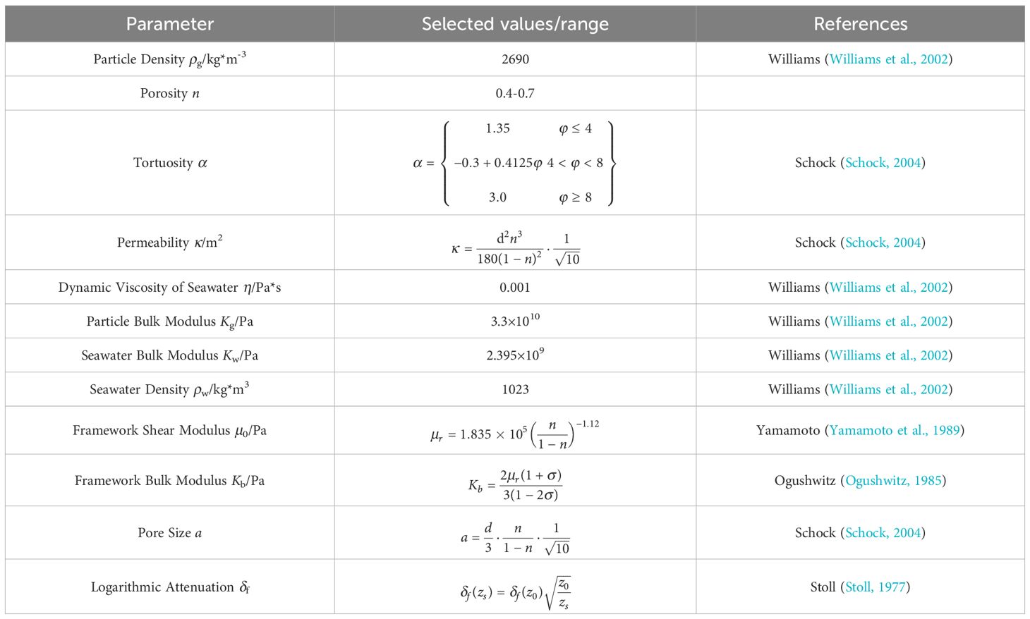
Table 1. Parameter values for the Biot-Stoll model.

Since the porosity n, sediment density ρ, and median grain size ϕ are interrelated through certain conversion relationships, it is necessary to analyze the sensitivity of these three parameters within the model to facilitate their selection. The results of the Sobol sensitivity analysis are shown in Figure 1. From the figure, it can be observed that both the total effect index and the main effect index of porosity are significantly higher than those of density and median grain size, indicating that the model is more sensitive to variations in porosity.

Figure 1

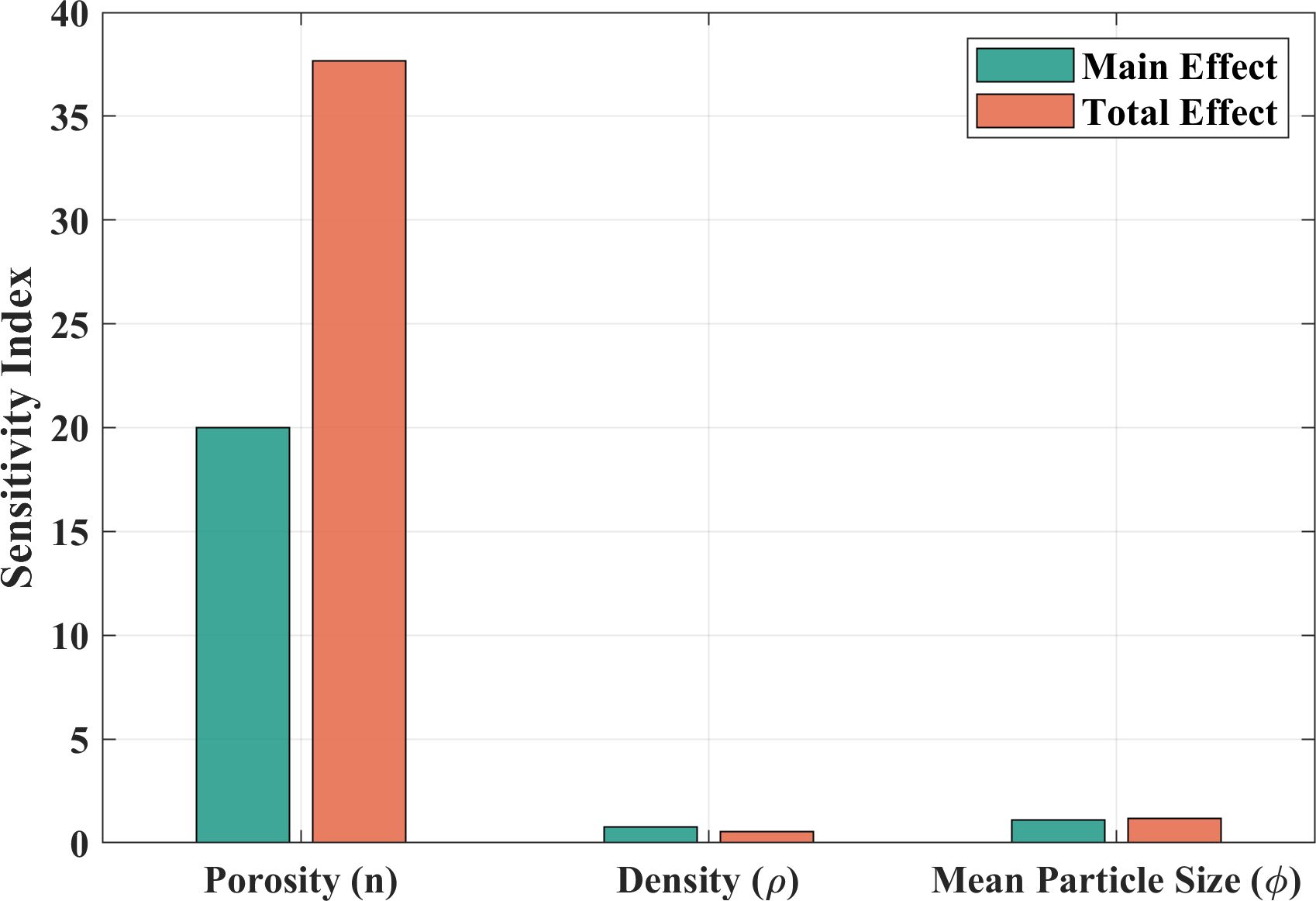
Figure 1. Sobol sensitivity analysis results chart.

2.2 PSO-BP neural network

The forward modeling process can be viewed as using the porosity input, passing through the underwater environment, to obtain the seafloor reflection coefficient. When the model becomes overly complex, solving the inverse problem to derive the underwater environment becomes extremely challenging. Therefore, the constructed PSO-BP neural network aims to simulate the inverse of the seafloor environment. In this study, a hybrid approach combining Particle Swarm Optimization (PSO) with Backpropagation (BP) algorithms is adopted. This method primarily seeks to overcome the issues associated with BP neural networks, such as high sensitivity to the initial weight values and a tendency to fall into local minima during training.

Furthermore, a novel inertia weight adjustment strategy is proposed, employing a nonlinear adaptive inertia weight ω as described by the Equation 1:

$\begin{array}{ll}\begin{array}{c}{\omega }^{(t)}={\omega }_{min}+({\omega }_{max}-{\omega }_{min})*{(1-g/G_k)}^{\alpha (t)}\\ \alpha (t)={\alpha }_{min}+({\alpha }_{max}-{\alpha }_{min})*(1-\gamma )\end{array}& (1)\end{array}$

In this formulation, ${\omega }^{(t)}$ denotes the inertia weight at the t-th iteration. The variable g represents the current iteration index, while $G_k$ denotes the maximum number of iterations. The $\alpha (t)$ is a time-varying nonlinear control parameter that modulates the rate of change of the inertia weight. The parameter γ is a constant regulating the variation of $\alpha (t)$; in the present context, γ=0.9. Compared to traditional PSO algorithms, the nonlinear adaptive inertia weight strategy presented in this paper causes the weight to vary nonlinearly with the number of iterations.

3 Methodology

3.1 Construction of the training dataset

In marine acoustics research, the Biot–Stoll model can be employed to simulate realistic seabed environments by calculating the seabed reflection coefficient based on thirteen physical parameters, including porosity. This model provides a comprehensive description of the acoustic properties of sediments; however, its structure is highly complex, making inverse problem solving particularly challenging. The core concept of this study is to develop a reverse environment of the Biot–Stoll model using a PSO–BP neural network, whereby the acoustic property parameters of sediments are inferred from the known seabed reflection coefficient. In this study, the selection of the porosity parameter n is of critical importance for the performance of the PSO-BP inversion network. This parameter directly affects the prediction accuracy and practical applicability of the model. To ensure the rationality and accuracy of the parameter, we comprehensively considered existing literature findings and empirical porosity values specific to the study region, establishing a porosity range from 0.4 to 0.7. To analyze the influence of porosity variations on the model’s predictive performance in more detail, a step size of 0.0006 was chosen, resulting in 501 discrete porosity values. Using these values, corresponding seafloor reflection coefficients were computed via the Biot-Stoll model, which served as the training dataset for network optimization. For different frequency scenarios, the training datasets were derived from this porosity range, with the seafloor reflection coefficients at the respective frequencies as input features and porosity as the output label for network training.

3.2 Construction of the PSO-BP network

To improve the realism and adaptability of the prediction model, environmental noise simulating actual underwater measurement conditions was incorporated into the training process at frequencies of 8 kHz and 100 kHz. Specifically, Gaussian noise with a standard deviation corresponding to 10% of the input data’s standard deviation was added to the seafloor reflection coefficient inputs. This step aimed to emulate measurement noise encountered in real seafloor reflection coefficient data, thereby enhancing the model’s robustness against environmental variability. The noisy reflection coefficients served as input features, with porosity as the output, for neural network training. To further assess the model’s accuracy and generalization capacity, the dataset was randomly shuffled prior to training, with 15% of the data reserved as a test set to evaluate prediction performance.

The neural network used in this study follows a standard feedforward structure, consisting of an input layer, a single hidden layer with 5 neurons, and an output layer. The network was trained using the Levenberg–Marquardt algorithm (trainlm), with the tansig activation function applied to the hidden layer and the purelin activation function applied to the output layer. The performance of the network was evaluated using the Mean Squared Error (MSE) loss function. Figure 2 presents the architecture of the neural network, including the layer composition, activation functions, and training settings in detail.

Figure 2

Figure 2. Neural network architecture.

The training results (shown in Figures 3a1, 3b1) display plots of sample number (horizontal axis) versus the predicted porosity obtained from the inverse model (vertical axis). The true porosity values, obtained via forward modeling, are plotted as the actual data, while the predicted values are derived from the trained neural network. The mean absolute percentage error (MAPE) remained within 1.3%, indicating high prediction accuracy. Additionally, error convergence plots were generated, where the number of iterations in the particle swarm optimization was plotted along the horizontal axis, and the model’s fitness (measured by mean square error) along the vertical axis. It was observed that the error reached its minimum after approximately 68 iterations at 8 kHz and 42 iterations at 100 kHz (Figures 3a2, 3b2). The training process then ceased, demonstrating effective convergence to an optimal minimum error state. These results confirm that, following initial iterative optimization, the model can reliably converge to a minimum-error solution, validating the stability and effectiveness of the employed methodology and algorithm for this application (Figures 3a3, 3b3).

Figure 3

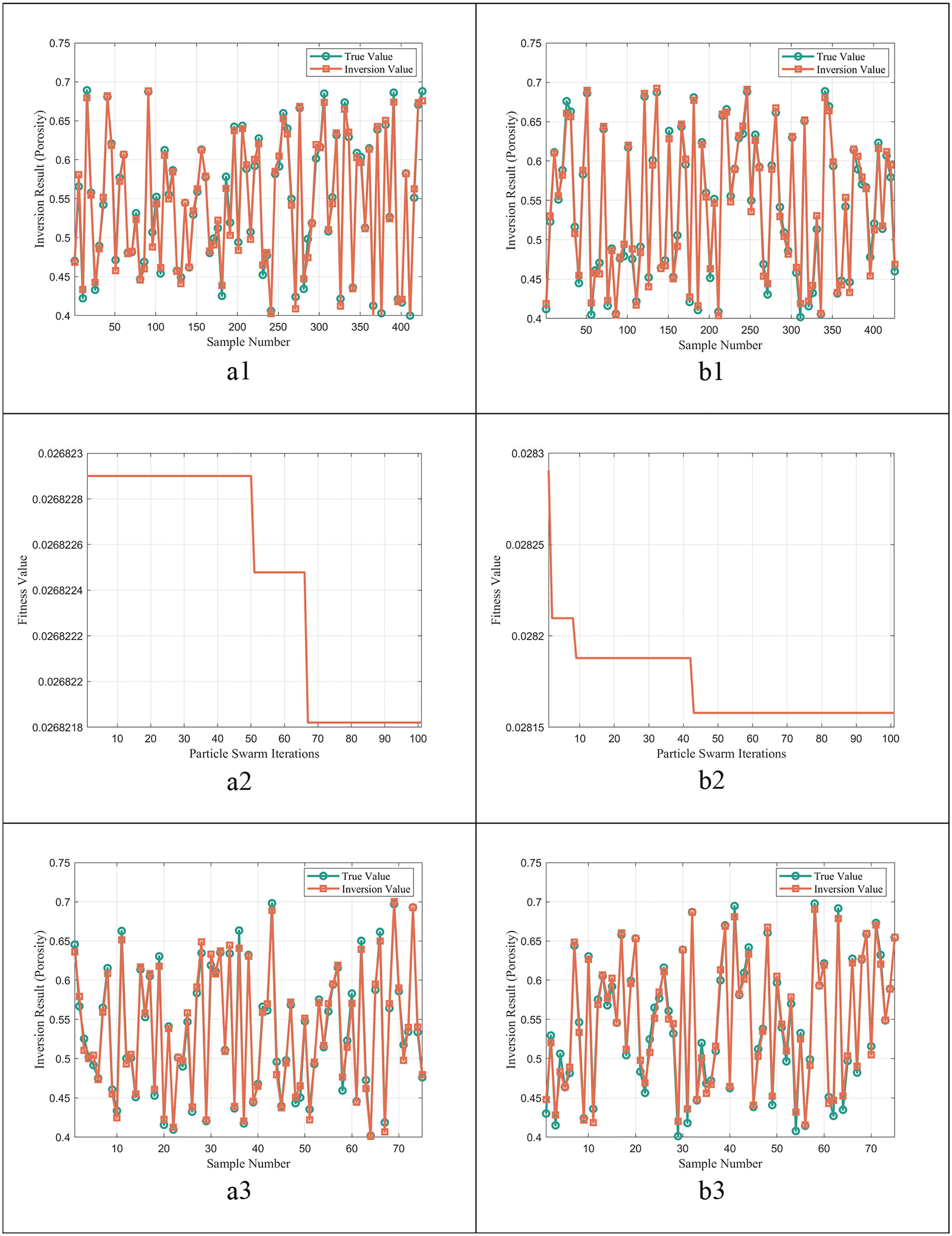
Figure 3. Inversion model training process under different frequency conditions: (a1) Training-set results at 8 kHz; (a2) Error variation at 8 kHz; (a3) Test-set results at 8 kHz; (b1) Training-set results at 100 kHz; (b2) Error variation at 100 kHz; (b3) Test-set results at 100 kHz.

4 Experimental data and inversion results

4.1 Data sources

The data used in this study originate from the project titled National Key Research and Development Program of China(2021YFF0501200). During the research cruise in the northern South China Sea, sediment core samples were collected and analyzed in the Laoshan laboratory. Laboratory measurements of sound speed, density, and porosity of the core samples were conducted under 100 kHz conditions. Additionally, in situ acoustic measurements of the seafloor sediments were performed using an underwater sediment acoustic in situ measurement system, providing seafloor sediment sound speed data at 8 kHz. These datasets serve to thoroughly validate the PSO-BP inversion model. By comparing laboratory measurements with in situ data as benchmarks, we evaluate the accuracy and applicability of the neural network in estimating actual sound speed under different frequency conditions.

4.2 Inversion results

This study is based on the inversion of acoustic parameters of seafloor sediments derived from the seafloor reflection coefficient, with detailed analysis conducted on parameters such as sound speed, porosity, and density within the upper 0–30 cm sediment layer. The sediment types include coarse silt, silty clay, sandy clay, sandy silt, clayey silt, and silted sand—covering six categories. Among these, the three most prevalent are silt-rich sand, clayey silt, and silted sand. The specific parameters are summarized in Table 2.

Table 2

Table 2. Surface sediment measurement data.

The seafloor reflection coefficient was calculated based on measured sound speed data at 100 kHz and 8 kHz frequencies, using the Equation 2:

$\begin{array}{ll}R=\frac{\rho v-{\rho }_w{v}_w}{\rho v+{\rho }_w{v}_w}& (2)\end{array}$

where $\rho$, $v$ are the measured density and sound speed of the sediment, and ${\rho }_w$=1023kg/m³ and $v_w$ = 1500m/s are the seawater density and sound speed, respectively. Based on the measured values, the reflection coefficient was first determined. Subsequently, the porosity was estimated through inversion of the reflection coefficient, and the sediment’s density and sound speed were calculated using Equations 3 and 4.

$\begin{array}{ll}\rho =n{\rho }_w+(1-n){\rho }_g& (3)\end{array}$

$\begin{array}{ll}v=\frac{{\rho }_w{v}_w(1+R)}{\rho (R-1)}& (4)\end{array}$

The results (Figure 4) indicate that the mean absolute percentage error (MAPE) for porosity is 2.39%, with a mean absolute error of 0.01. In addition, the average absolute percentage errors for density and sound speed are 1.01%, with mean absolute errors of 17.29 kg/m³ and 15.27 m/s, respectively. These findings validate the accuracy and reliability of the developed inversion network.

Figure 4

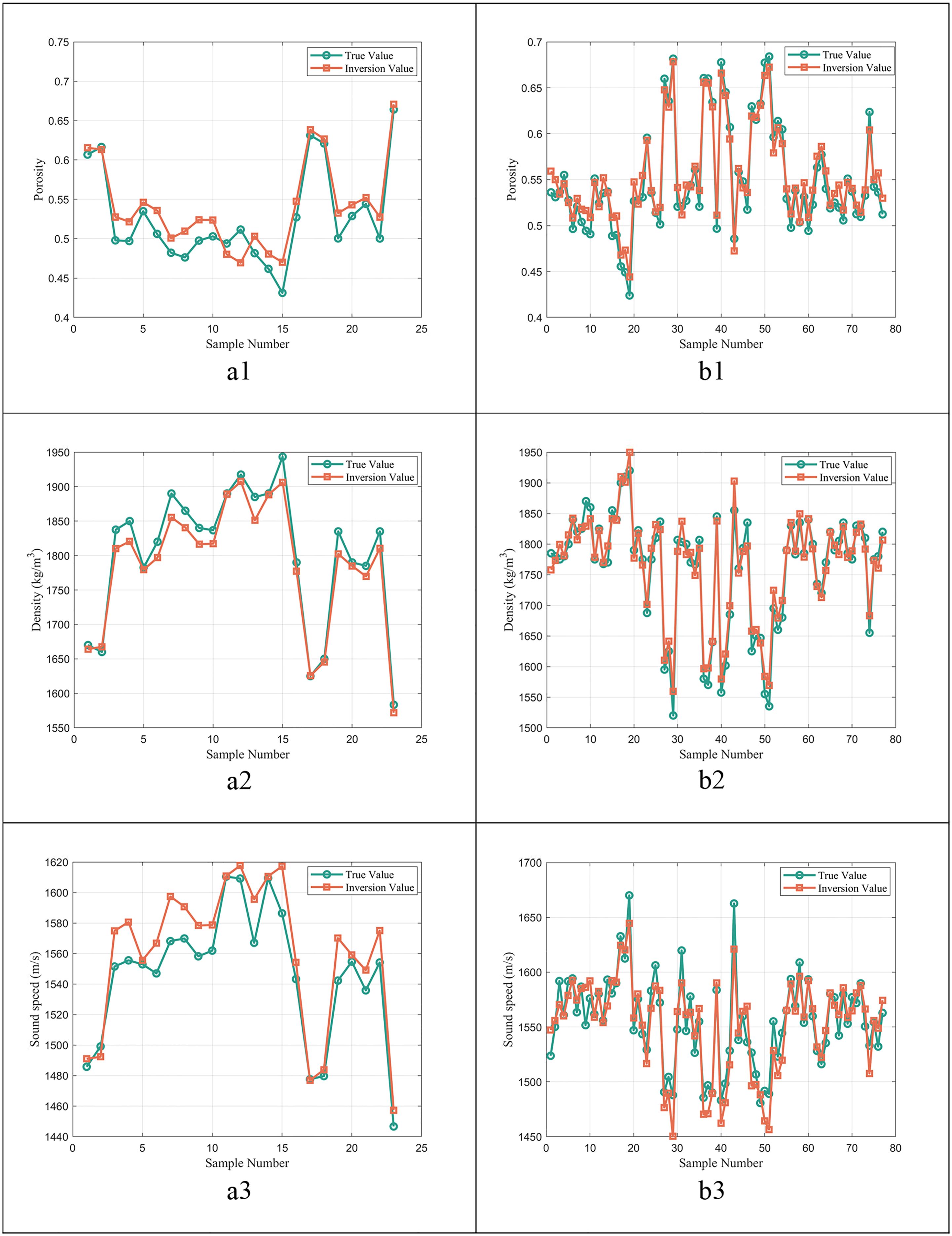
Figure 4. Inversion results under different frequency conditions: (a1) Porosity inversion results at 8 kHz; (a2) Density inversion results at 8 kHz; (a3) Velocity inversion results at 8 kHz; (b1) Porosity inversion results at 100 kHz; (b2) Density inversion results at 100 kHz; (b3) Velocity inversion results at 100 kHz.

5 Inversion errors and discussion

In sediment acoustic parameter inversion, model error serves as a key indicator of inversion accuracy. This study validates the inversion model using data at both 8 kHz and 100 kHz frequencies, analyzing the applicability of the method for three sediment types—Silted Sand, Sandy Siltt, and Clayey Silt—under different frequency conditions for parameters such as sound speed, density, and porosity. The results (Table 3) demonstrate that the inversion errors across these parameters are relatively small at both frequencies.

Table 3

Table 3. Error results for different sediment types.

Overall, errors at 100 kHz tend to be lower, whereas at 8 kHz, the maximum errors—particularly in porosity—are generally higher. Among the three sediment types, Silted Sand shows the highest porosity errors, with maximum values of 5.41% at 100 kHz and 6.36% at 8 kHz. For Silted Sand, the maximum errors in sound speed are 1.62% (8 kHz) and 2.50% (100 kHz), while the maximum density errors are 1.60% and 2.57%, respectively. For Sandy Silt, the maximum errors in sound speed are 1.58% (8 kHz) and 2.13% (100 kHz), with density errors of 1.55% and 2.09%. These findings suggest that the inversion of sound speed tends to be more accurate at 8 kHz, while density inversions are relatively more stable at 100 kHz.

Regarding minimum errors, both frequencies exhibit very low error margins: for Silted Sand, the minimum density errors are 0.02% (8 kHz) and 0.04% (100 kHz); for Sandy Silt, 0.08% (8 kHz) and 0.01% (100 kHz). In contrast, Clayey Silt shows a wider error distribution, with porosity errors ranging from 0.40% to 3.13%, indicating that this sediment type has higher sensitivity to frequency-dependent effects.

Further analysis of the average errors reveals that all three sediment types maintain mean errors around 1%, indicating good overall stability of the inversion model. Specifically, the mean errors for Silted Sand are 0.93% (8 kHz) and 0.76% (100 kHz); for Sandy Silt, 0.83% (8 kHz) and 0.78% (100 kHz); and for Clayey Silt, 1.41% (at 100 kHz). Notably, the inversion accuracy for Clayey Silt appears to be somewhat lower at higher frequencies.

Distinct variability among sediment types is evident; Silted Sand and Sandy Silt exhibit larger frequency-dependent errors in parameters such as sound speed and porosity, whereas Clayey Silt demonstrates more consistent, lower errors—likely due to more homogeneous structures that favor stable high-frequency parameter inversions. For sediments with less uniform particle distribution, such as Silted Sand and Sandy Silt, more complex correction methods may be necessary to mitigate local fluctuations and errors.

Analyzing errors based on porosity, density, and sound speed data, the results show that the average relative error in porosity inversion at 100 kHz (2.06%) is significantly lower than at 8 kHz (3.79%), indicating that higher frequency signals can better capture porosity variations and improve inversion accuracy. For density, the average relative errors at both frequencies are low (0.865% at 8 kHz and 0.813% at 100 kHz), demonstrating good stability, though the overall mean absolute errors (approximately 14.9) are relatively large—possibly affected by environmental noise during actual measurements. Similarly, for sound speed, the errors at both frequencies are comparable, with average relative errors around 0.85%, but the absolute errors (approximately 15 m/s) suggest room for further improvement (Table 4).

Table 4

Table 4. Error results for different data types.

6 Conclusion

This study employed Biot theory and the Biot-Stoll model to generate datasets for training the PSO-BP neural network and constructed an inversion framework based on this hybrid model. The validation was performed using surface data collected from both measured samples and in situ sampling points in the northwestern South China Sea. The results demonstrate the high accuracy of the developed PSO-BP inversion network. Specifically, when inverting parameters such as porosity, density, and sound speed using laboratory data at 100 kHz, the maximum mean absolute percentage error (MAPE) was 2.3%. For in situ measurement data, the maximum error increased to 3.8%. The comparison between high-frequency laboratory data (100 kHz) and mid-frequency in situ data (8 kHz) confirms the method’s feasibility and robustness across different frequency conditions. These findings highlight the potential of the proposed approach for accurate and flexible marine sediment parameter inversion in complex underwater environments.

Data availability statement

The original contributions presented in the study are included in the article/supplementary material. Further inquiries can be directed to the corresponding authors.

Author contributions

LJ: Validation, Writing – review & editing, Project administration, Supervision, Data curation, Visualization, Methodology, Formal analysis, Investigation, Conceptualization, Software, Resources, Writing – original draft. JL: Conceptualization, Writing – review & editing, Resources, Formal analysis, Project administration, Methodology. WJ: Visualization, Investigation, Conceptualization, Writing – review & editing, Validation, Supervision. CL: Resources, Software, Validation, Formal analysis, Writing – review & editing, Project administration. LC: Writing – review & editing, Investigation, Data curation, Visualization, Project administration. KF: Project administration, Funding acquisition, Formal analysis, Resources, Writing – review & editing, Data curation, Methodology, Validation. LS: Methodology, Writing – review & editing, Project administration, Visualization, Software. KG: Supervision, Data curation, Methodology, Investigation, Writing – review & editing.

Funding

The author(s) declare financial support was received for the research and/or publication of this article. China Geological Survey Projects (Project No.: DD20230592); National Key Research and Development Program of China (Project No.: 2021YFF0501200); China Geological Survey Projects (Project No.: DD20242841).

Acknowledgments

TData and sample collection were supported by the National Key Research and Development Program of China (Project No.: 2021YFF0501200), and data processing and manuscript preparation were supported by the China Geological Survey Projects (Project No.: DD20230592). The data acquisition was conducted onboard the R/V XiangYang Hong 01 by The First Institute of Oceanography, Ministry of Natural Resources, China.

Conflict of interest

The authors declare that the research was conducted in the absence of any commercial or financial relationships that could be construed as a potential conflict of interest.

Generative AI statement

The author(s) declare that no Generative AI was used in the creation of this manuscript.

Any alternative text (alt text) provided alongside figures in this article has been generated by Frontiers with the support of artificial intelligence and reasonable efforts have been made to ensure accuracy, including review by the authors wherever possible. If you identify any issues, please contact us.

Publisher’s note

All claims expressed in this article are solely those of the authors and do not necessarily represent those of their affiliated organizations, or those of the publisher, the editors and the reviewers. Any product that may be evaluated in this article, or claim that may be made by its manufacturer, is not guaranteed or endorsed by the publisher.

References

Amiri-Simkooei A. R., Koop L., Reijden K. J.v. d., Snellen M., and Simons D. G. (2019). Seafloor characterization using multibeam echosounder backscatter data: methodology and results in the North Sea. Geosciences 9, 2925. doi: 10.3390/geosciences9070292

Crossref Full Text | Google Scholar

An Z., Zhang J., and Xing L. (2020). Inversion of oceanic parameters represented by CTD utilizing seismic multi-attributes based on convolutional neural network. J. Ocean Univ. China 19, 1283–12915. doi: 10.1007/s11802-020-4133-x

Crossref Full Text | Google Scholar

Batchelor C. L., Montelli A., Ottesen D., Evans J., Dowdeswell E. K., Christie F. D. W., et al. (2020). New insights into the formation of submarine glacial landforms from high-resolution Autonomous Underwater Vehicle data. Geomorphology 370, 107396. doi: 10.1016/j.geomorph.2020.107396

Crossref Full Text | Google Scholar

Chapman N.R. (1983). Modeling ocean-bottom reflection loss measurements with the plane-wave reflection coefficient. J. Acoustical Soc. America 73, 1601–16075. doi: 10.1121/1.389424

Crossref Full Text | Google Scholar

Chiu L. Y. S., Chang A., Lin Y.-T., and Liu C.-S. (2014). Estimating geoacoustic properties of surficial sediments in the North Mien-Hua Canyon region with a chirp sonar profiler. IEEE J. Oceanic Eng. 40, 222–2365. doi: 10.1109/JOE.2013.2296362

Crossref Full Text | Google Scholar

De C. and Chakraborty B. (2011). Model-based acoustic remote sensing of seafloor characteristics. IEEE Trans. Geosci. Remote Sens. 49, 3868–38775. doi: 10.1109/TGRS.2011.2139218

Crossref Full Text | Google Scholar

Dettmer J., Dosso S. E., and Holland C. W. (2008). Joint time/frequency-domain inversion of reflection data for seabed geoacoustic profiles and uncertainties. J. Acoustical Soc. America 123, 1306–13175. doi: 10.1121/1.2832619

PubMed Abstract | Crossref Full Text | Google Scholar

Dettmer J., Holland C. W., and Dosso S. E. (2009). Analyzing lateral seabed variability with Bayesian inference of seabed reflection data. J. Acoustical Soc. America 126, 56–695. doi: 10.1121/1.3147489

PubMed Abstract | Crossref Full Text | Google Scholar

Gassner L., Gerach T., Hertweck T., and Bohlen T. (2019). Seismic characterization of submarine gas-hydrate deposits in the Western Black Sea by acoustic full-waveform inversion of ocean-bottom seismic data. Geophysics 84, B311–B324. doi: 10.1190/geo2018-0622.1

Crossref Full Text | Google Scholar

Haris K., Chakraborty B., De C., Prabhudesai R. G., and Fernandes W. (2011). Model-based seafloor characterization employing multi-beam angular backscatter data—A comparative study with dual-frequency single beam. J. Acoustical Soc. America 130, 3623–36325. doi: 10.1121/1.3658454

PubMed Abstract | Crossref Full Text | Google Scholar

Huang B., Li J., Zhou Q., Li X., Liu L., Gao S., et al. (2022). Research on inversion technology of physical properties parameters of seafloor sediments based on sub-bottom profile: Taking the Bohai Sea submarine pipeline route as an example. Haiyang Xuebao 44, 156–1645. Available online at: https://kns.cnki.net/kcms2/article/abstract?v=bugI047JRxghiqp1DpeVhcrlVdo5SOJbv4pPWHBpSngBxTEa59NxHvprgQAHECVctzPumuk1Ftiv-UAw1BU4O-PBozIt3yG_lTs5_VrkX5jUQXYMuFncGYqGcgdD-lmIcY4wbSWUZs_jPiqPhIeXD7lBXk8_pJwtUKBcusuUb6cACl-DKtN4iQ==&uniplatform=NZKPT&language=CHS

Google Scholar

Huang Y., Xiang Y., Zhao R., and Cheng Z. (2020). Air quality prediction using improved PSO-BP neural network. IEEE Access 8, 99346–99353. doi: 10.1109/Access.6287639

Crossref Full Text | Google Scholar

Jackson D. R., Winebrenner D. P., and Ishimaru A. (1986). Application of the composite roughness model to high-frequency bottom backscattering. J. acoustical Soc. America 79, 1410–14225. doi: 10.1121/1.393669

Crossref Full Text | Google Scholar

Li X., Liu L., Huang B., Zhou Q., and Zhang C. (2024). Erosional and depositional features along the axis of a canyon in the northern south China sea and their implications: insights from high-Resolution AUV-Based geophysical data. J. Mar. Sci. Eng. 12, 5995. doi: 10.3390/jmse12040599

Crossref Full Text | Google Scholar

Mackenzie K. V. (1960). Reflection of sound from coastal bottoms. J. Acoustical Soc. America 32, 221–231. doi: 10.1121/1.1908019

Crossref Full Text | Google Scholar

Ogushwitz P. R. (1985). Applicability of the Biot theory. I. Low-porosity materials. J. Acoustical Soc. America 77, 429–440. doi: 10.1121/1.391863

Crossref Full Text | Google Scholar

Schock S. G. (2004). A method for estimating the physical and acoustic properties of the sea bed using chirp sonar data. IEEE J. Oceanic Eng. 29, 1200–1217. doi: 10.1109/JOE.2004.841421

Crossref Full Text | Google Scholar

Sternlicht D. D. and Moustier C. P. (2003). Time-dependent seafloor acoustic backscatter (10–100 kHz). J. acoustical Soc. America 114, 2709–27255. doi: 10.1121/1.1608018

PubMed Abstract | Crossref Full Text | Google Scholar

Stoll R. D. (1977). Acoustic waves in ocean sediments. Geophysics 42, 715–725. doi: 10.1190/1.1440741

Crossref Full Text | Google Scholar

Tan P., Sun M., Qin J., and Yang D. (2023). Geoacoustic inversion in shallow water by matching vertical particle velocity. Acta Acustica 48, 70–825. doi: 10.15949/j.cnki.0371-0025.2023.01.002

Crossref Full Text | Google Scholar

Wang J., Tang Y., Li S., Lu Y., Li J., Liu T., et al. (2024). The Haidou-1 hybrid underwater vehicle for the Mariana Trench science exploration to 10,908 m depth. J. Field Robotics 41, 1054–10795. doi: 10.1002/rob.22307

Crossref Full Text | Google Scholar

Wang T., Su L., Ren Y., Wang W., and Ma L. (2021). Application of the sound speed profile and sound source location in shallow waters. Harbin Eng. Univ. J. 42, 1133–11395. Available online at: https://kns.cnki.net/kcms2/article/abstract?v=bugI047JRxjuoW4E5n3eLzWS6akKmCQwFGVCSe6AktYoE2VMFw04snBktRBa4ZV4m6W8

Google Scholar

Wang Z., Ma Y., Kan G., Liu B., Zhou X., and Zhang X. (2023). An inversion method for geoacoustic parameters in shallow water based on bottom reflection signals. Remote Sens. 15, 32375. doi: 10.3390/rs15133237

Crossref Full Text | Google Scholar

Williams K. L., Jackson D. R., Thorsos E. I., Tang D., and Schock S. G. (2002). Comparison of sound speed and attenuation measured in a sandy sediment to predictions based on the Biot theory of porous media. IEEE J. oceanic Eng. 27, 413–4285. doi: 10.1109/JOE.2002.1040928

Crossref Full Text | Google Scholar

Yamamoto T., Trevorrow M. V., Badiey M., and Turgut A. (1989). Determination of the seabed porosity and shear modulus profiles using a gravity wave inversion. Geophysical J. Int. 98, 173–1825. doi: 10.1111/j.1365-246X.1989.tb05522.x

Crossref Full Text | Google Scholar

Zhang J., Chen C., Wu C., Kou X., and Xue Z. (2024). Storage quality prediction of winter jujube based on particle swarm optimization-backpropagation-artificial neural network (PSO-BP-ANN). Scientia Hortic. 331, 112789. doi: 10.1016/j.scienta.2023.112789

Crossref Full Text | Google Scholar

Zhu H., Cui Z., Liu J., Jiang S., Liu X, and Wang J. (2023). A method for inverting shallow sea acoustic parameters based on the backward feedback neural network model. J. Mar. Sci. Eng. 11, 13405. doi: 10.3390/jmse11071340

Crossref Full Text | Google Scholar