Estimation of surface duct parameters using AIS data based on Bayesian inversion method

Automatic Identification System (AIS) operates within a very high frequency (VHF) maritime mobile band, which could be impacted by surface duct seriously. Utilizing AIS signals for atmospheric duct inversion is a relatively new technique in passive remote sensing. This study employs the Bayesian method to conduct inversion of maritime surface ducts based on AIS signals, categorizing surface ducts into surface-based and elevated-surface ducts. Initially, preliminary data on surface-based duct and elevated-surface duct parameters are acquired from historical sounding data, followed by correlation analysis and probability density distribution fitting of these surface duct parameters. Subsequently, the inversion method steps are provided, and using the same measured AIS data, the likelihood function and posterior probability are calculated by directly employing historical samples and samples generated using Latin Hypercube Sampling (LHS), to accomplish the estimation of surface duct parameters. Directly utilizing historical samples and LHS-generated samples for Bayesian inversion can consistently and accurately yield results with an elevated-surface duct, with the latter being slightly more accurate than the former. The root mean square errors for the AIS path loss, calculated using the inverted elevated-surface duct parameters, are 5.9 dB and 4.4 dB when compared with the measured data. In contrast, the error calculated from the inverted surface-based duct parameters is 21.9 dB.

1 Introduction

Atmospheric ducts facilitate the trans-horizon propagation of radio systems, including radar and communication systems, and can lead to interference between systems (Kang et al., 2017). To evaluate the performance of these systems, it is essential to obtain precise atmospheric duct environmental parameters. Atmospheric ducts are typically categorized into three types: evaporation duct, surface duct, and elevated duct. Evaporation ducts are almost perpetually present over the sea, primarily influences radio waves above approximately 2GHz (Yang et al., 2022a; Yang et al., 2022b; Guo et al., 2023). The occurrence probability of surface duct and elevated duct is approximately 20-60% (Hao et al., 2022), which can affect radio waves in the VHF band and above (Sirkova, 2022; Sirkova, 2023). Of all the atmospheric duct types, the surface duct has the most substantial impact on maritime radio systems, including the Automatic Identification System (AIS). AIS was introduced to help improve maritime safety and avoid ship collisions around 2000. As a VHF system, the maximum range of AIS communications is normally governed by line-of-sight propagation. However, under suitable atmospheric duct conditions, particularly surface ducts, AIS signals can generate a trans-horizon propagation effect (ITU-R M.2123, 2007; ITU-R M.1371-5, 2014). Bruin (2016) studied the environmental impact on radio wave propagation of the AIS and coastal radar in the operational area of the Netherlands Coastguard, by using Numerical Weather Prediction (NWP) and the parabolic equation. Zhang (Zhang et al., 2022) investigated the propagation characteristics of AIS signals under different atmospheric refraction conditions, using measured data to verify the significant impact of low-altitude atmospheric ducts on actual VHF-band AIS signals in maritime environments.

Most studies on marine atmospheric duct inversion are based on radar sea clutter (Gerstoft et al., 2003; Douvenot et al., 2010; Karimian et al., 2011; Compaleo et al., 2018), including methods based on Bayesian inversion (Yardim et al., 2006); however, obtaining these data is not straightforward. Therefore, relevant researchers are continuously exploring the use of other signal sources for atmospheric duct inversion studies, such as GNSS signals (Lowry et al., 2002; Wang et al., 2013; Liao et al., 2018), AIS signals, etc. Since all maritime AIS transmitters are within the surface duct height range, and an AIS receiver installed along the coastline also falls within this range, the surface duct has a significant impact on AIS signal propagation, whereas elevated ducts with higher trapping layers have minimal influence. Therefore, AIS is suitable for retrieving marine surface duct parameters. Tang (Tang et al., 2019) simulated the surface-based duct parameters estimation from AIS signal using the Levy flight quantum-behaved particle swarm optimization algorithm. Huang (Huang et al., 2023) utilized simulated AIS data to conduct a comparative analysis of the inversion results of atmospheric duct using different global optimization algorithms, including genetic algorithm, simulated annealing algorithm, and particle swarm optimization algorithm. Han (Han et al., 2022b) first established an AIS-based model for diagnosing atmospheric duct types using artificial intelligence, and then employed deep learning to perform inversion of atmospheric duct parameters.

By utilizing historical statistics of surface duct as prior information, we propose for the first time a Bayesian inversion method for surface duct based on AIS, and further subdivide surface duct into surface-based duct and elevated-surface duct for inversion and comparative analysis. Compared to previous global optimization algorithms and artificial intelligence, the advantage of Bayesian inversion based on AIS signals lies in obtaining atmospheric duct parameters while simultaneously deriving the probability distribution of these parameters. The Bayesian inversion method is capable of providing the probability distribution of parameters because it consistently treats unknown variables as random variables with uncertainty, and representing the state uncertainty through probability distributions. In the following Section 2, the probability distribution of surface duct parameters is provided. Section 3 describes the methodological steps for inverting surface duct parameters using AIS signals with a Bayesian approach. Section 4 presents inversion examples and analyses under different conditions. A conclusion is drawn in Section 4.

2 Probability density of the surface duct parameters

2.1 Surface duct types and parameters

Refraction refers to the bending of radio waves as they traverse different transmission media. The tropospheric media are characterized by their index of refraction, refractivity, or modified refractivity. The refractivity, represented by N, can be determined using simple formulas that incorporate temperature, pressure, and humidity data (ITU-R P.453-10, 2012):

$\begin{array}{ll}N=(n-1)\times {10}^6=\frac{77.6}{T}(P+4810\frac{e}{T})\begin{array}{cc}& (\text{N}-\text{units})\end{array}& (1)\end{array}$

where n is the index of refraction, P is atmospheric pressure (hPa), e is water vapor pressure (hPa), and T is absolute temperature (K). The modified refractivity M is defined such that it allows for the consideration of the Earth as if it were a hypothetically flat surface:

$\begin{array}{ll}M=N+0.157z& (2)\end{array}$

where z is the height above the surface in meters.

A ducting layer characterized by a negative M gradient, which consequently may generate a tropospheric radio-duct if the layer is sufficiently thick compared with the wavelength. Surface ducts are classified into surface-based duct (SBD) and elevated-surface duct (ESD) with a base layer, as shown in Figure 1. According to the ITU-R P.310 (Definitions of terms relating to propagation in non-ionized media) definition of surface duct and elevated duct terminology, it is evident that surface ducts encompass the two types depicted in Figure 1 (ITU-R P.310-10, 2019). Nonetheless, there remains confusion surrounding the terminology for these two types of surface ducts. In ITU-R P.453, Figure 1a is referred to as a surface duct, while Figure 1b is called an elevated-surface duct. Some literature (Mentes and Kaymaz, 2007; Huang et al., 2023; Sirkova, 2023) refers to Figure 1a as a surface duct and Figure 1b as a surface-based duct. To avoid confusion regarding inclusion relationships and terminology, this paper designates Figure 1a as a surface-based duct and Figure 1b as an elevated-surface duct.

Figure 1

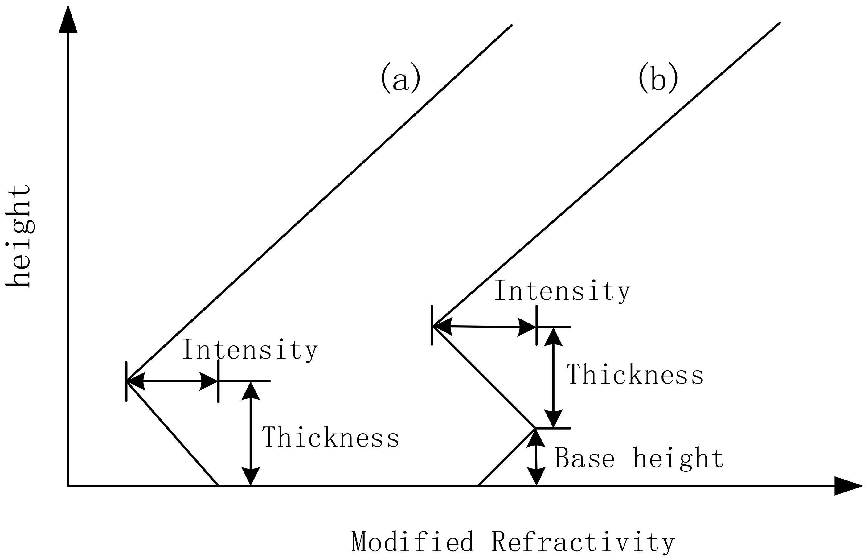
Figure 1. Surface duct types and parameters. (a) Surface-based duct; (b) Elevated-surface duct.

Elevated-surface duct consists of three basic parameters: duct base height, duct height, and duct intensity. The base height of the surface-based duct is zero, with two variable parameters: duct height and duct intensity. Assuming the positive gradient value in the modified refractivity profile of the surface duct is 0.118 M-units/m, which equals the gradient under standard atmospheric conditions, the surface-based duct profile can be calculated using the following equation (Han et al., 2022b):

$\begin{array}{ll}M(z)=\{\begin{array}{c}{M}_0-\frac{M_d}{z_t}z0\le z\le z_t\\ M_0-M_d+0.118zz\ge z_t\end{array}& (3)\end{array}$

where z is height, zt is the duct height, M_d is the duct intensity, and M₀ is modified refractivity of ground or sea surface. The variation of M₀ has little effect on radio wave propagation and can be set as a fixed value. The profile of an elevated-surface duct can be expressed as:

$\begin{array}{ll}M(z)=\{\begin{array}{ll}{M}_0+0.118z\hfill & 0\le z\le z_b\hfill \\ M{0}_{+}0.118z_b-\frac{M_d}{z_t}(z-z_b)\hfill & z_b\le z\le z_b+z_t\hfill \\ M_0-M_d+0.118(z-z_b-z_t)\hfill & z\ge z_b+z_t\hfill \end{array}& (4)\end{array}$

where zb is the duct base height.

2.2 Statistical distribution of surface duct parameters

Radiosonde data is the primary source of statistical data for atmospheric duct parameters, with over 600 radio sounding stations worldwide conducting measurements at 00:00 and 12:00 UTC daily. A radiosonde directly measures atmospheric temperature, humidity, and pressure data at various altitudes. From these measurements, the modified refractivity profile can be calculated using Equations 1, 2, facilitating the determination of the atmospheric duct type and the computation of its parameters.

This study utilizes five years (2015-2019) of radiosonde data from the region spanning 110°-140°E longitude and 10°-45°N latitude, obtaining a total of 17,534 surface duct samples. The base height distribution of the surface duct is shown in Figure 2, where a subplot is used to display the magnified content within the red rectangular box. The surface duct type with a base height of zero is the surface-based duct. Among these, 16,138 samples are surface-based ducts, while 1,396 samples are elevated-surface ducts.

Figure 2

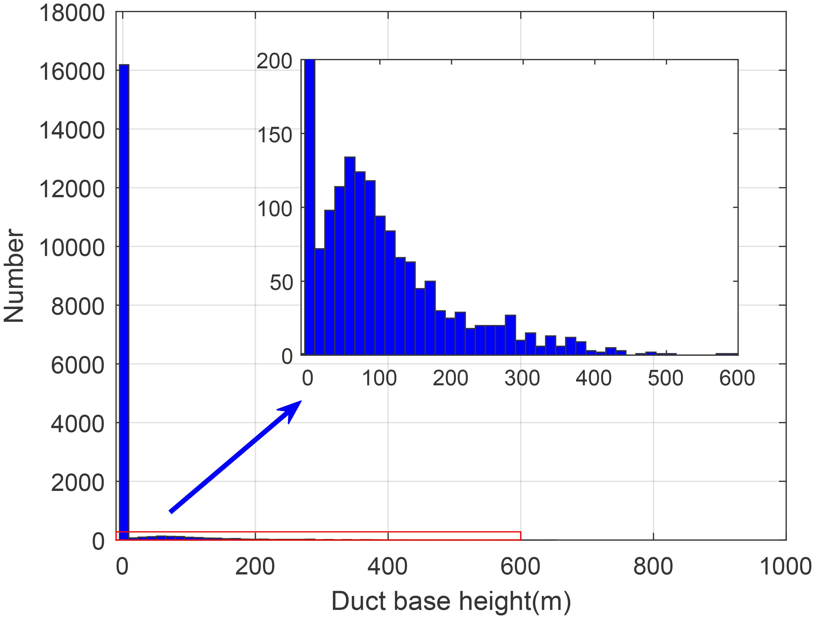
Figure 2. Base height distribution of the surface duct.

To facilitate the sampling of surface duct parameters during Bayesian inversion, the probability density distributions of these parameters were fitted using normal, lognormal, exponential, gamma, Rayleigh, and Poisson distribution functions. The results indicate that the surface duct parameters conform to a gamma distribution. The probability density of surface duct height and intensity without a base layer is shown in Figure 3, while the probability density of surface duct thickness, base height, and intensity with a base layer is shown in Figure 4. The histogram in the figure represents the measurement results, while the red curve shows the fitted probability density function. The fitting parameters and their values are listed in Table 1.

Figure 3

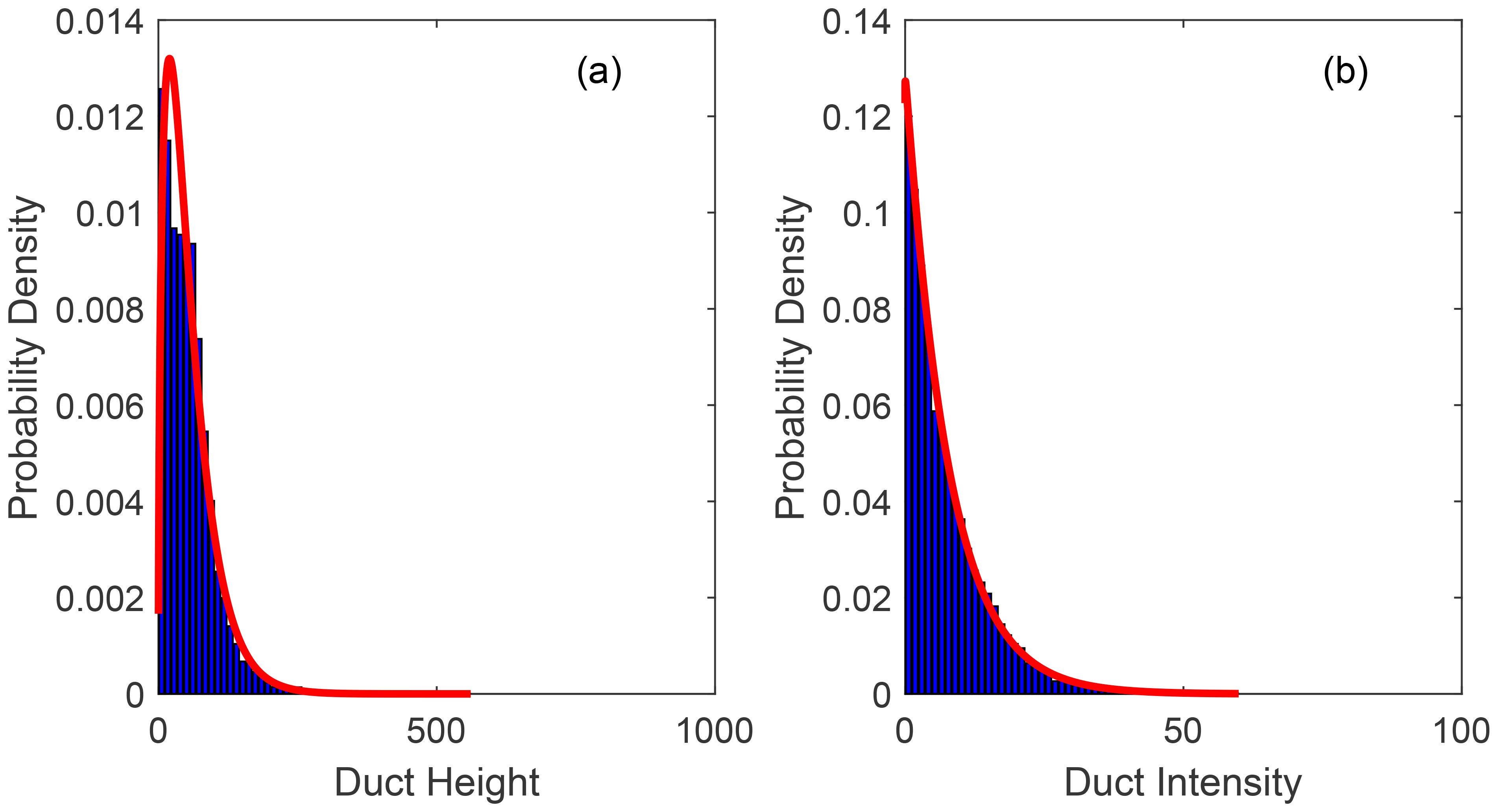
Figure 3. Surface-based duct parameters. (a) Duct height; (b) Duct intensity.

Figure 4

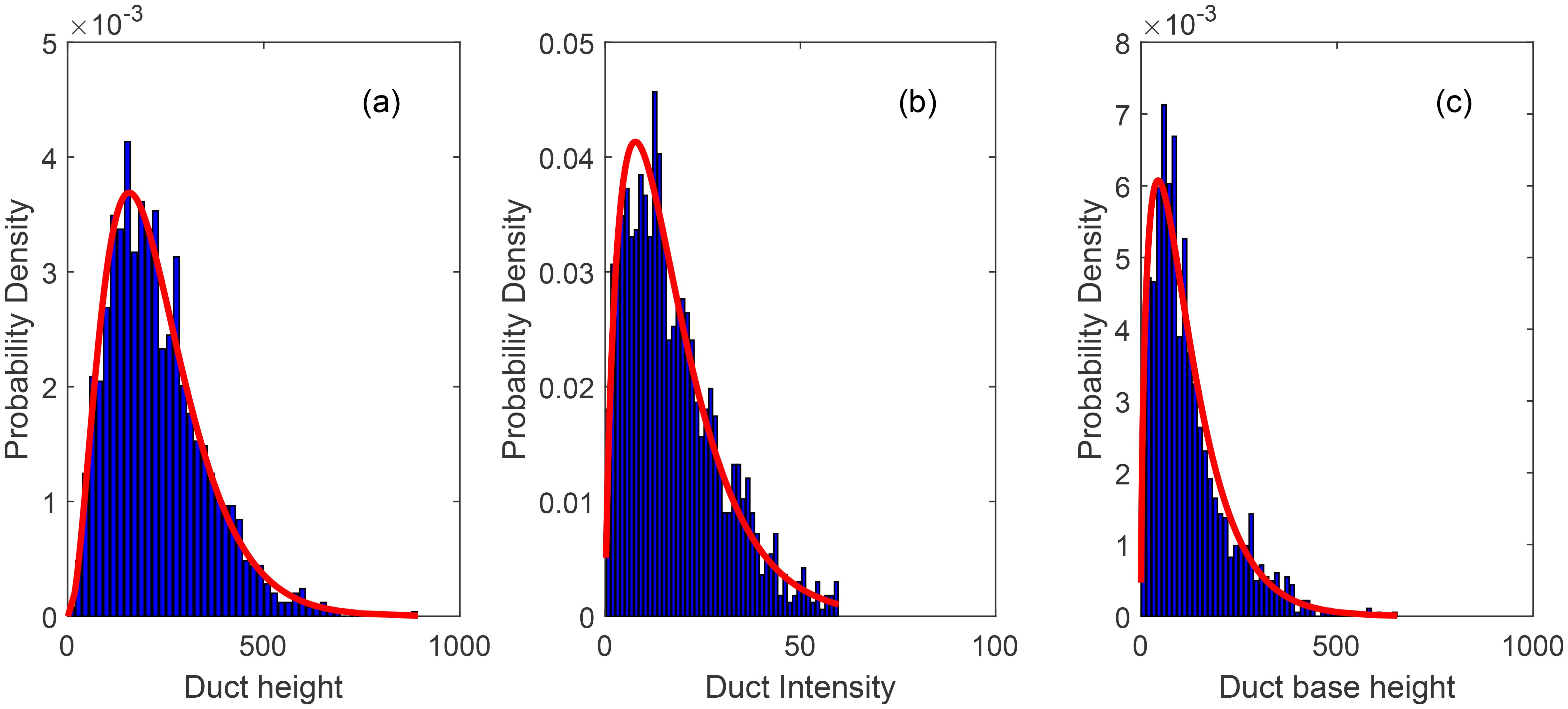
Figure 4. Elevated-surface duct. (a) Duct height; (b) Duct intensity; (c) Duct base height.

Table 1

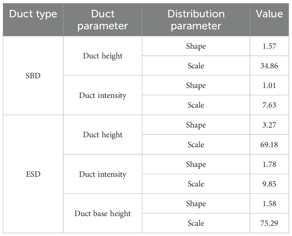
Table 1. Parameter distribution table of surface duct.

The correlation coefficient between the duct height and duct intensity parameters of the SBD is -0.05, indicating no significant correlation. The correlation coefficient matrix of ESD parameters (duct height, duct intensity, and duct base height) is:

$\begin{array}{ll}{\rho }_{\text{ESD}}=\left[\begin{array}{ccc}1& 0.598& 0.817\\ 0.598& 1& 0.593\\ 0.817& 0.593& 1\end{array}\right]& (5)\end{array}$

According to the statistical results of surface ducts, it can be seen that:(1) The proportion of SBD in surface ducts is significantly higher than that of ESD, with the former being approximately an order of magnitude greater than the latter; (2) The mean duct height of the SBD is 54.8m, with a mean intensity of 7.7 M-unit. The mean duct height of the ESD is 226.3m, with a mean intensity of 17.6 M-unit; (3) Among the normal distribution, log-normal distribution, exponential distribution, gamma distribution, Rayleigh distribution, and Poisson distribution, the parameters of SBD and ESD better conform to the gamma distribution; (4) The duct height and intensity of SBD are mutually independent, whereas the ESD’s duct height and intensity are correlated, demonstrating a moderate degree of association.

3 Bayesian inverse method of surface duct parameters using AIS data

Bayesian theorem states that the posterior probability can be obtained from the prior probability and the likelihood function. Based on the Bayesian theorem, an inversion method can be developed to monitor surface duct parameters with AIS observational data. In this method, the prior probability of surface duct parameters is initially obtained from historical data. Subsequently, the likelihood function of these parameters is calculated using the prior probability and AIS measurement data. Following this, the posterior probability of the surface duct parameters is determined based on the prior probability and the likelihood function. Ultimately, the posterior probability can be used to obtain predictive results of the model parameters and analyze the uncertainty of these results. The main steps of Bayesian inversion for surface duct parameters based on AIS data are as follows:

(1) The surface duct parameters are obtained according to the historical sounding data, and the probability distribution of the surface duct parameters is statistically obtained.

(2) The probability distribution of surface duct parameters is fitted to obtain the probability distribution function, and the sample of surface duct parameters is generated by LHS according to the probability distribution function.

(3) The measured AIS path loss is calculated according to the received power of AIS.

(4) Based on the surface duct parameter samples and the forward model, the simulation calculates the path loss for AIS corresponding to various samples.

(5) Based on the measured and simulated AIS path loss, the likelihood function p(d|m) of surface duct parameters under the measured AIS path loss condition is calculated.

(6) Applying Bayes’ theorem to calculate the posterior probability distribution of surface duct parameters p(m|d). p(m|d) is proportional to the product of the likelihood function and the prior probability, expressed as:

$\begin{array}{ll}p(m|d)\propto p(d|m)p(m)& (6)\end{array}$

(7) Parameter estimation and uncertainty analysis through posterior probability distribution of surface duct parameters.

The overall procedure of the surface duct inversion is depicted in the flowchart of Figure 5. Surface duct parameter samples can be selected from historical samples or those generated by LHS. The former has the advantage of ensuring that the inversion results have been observed historically, while the latter offers the benefit of controllable sample quantity.

Figure 5

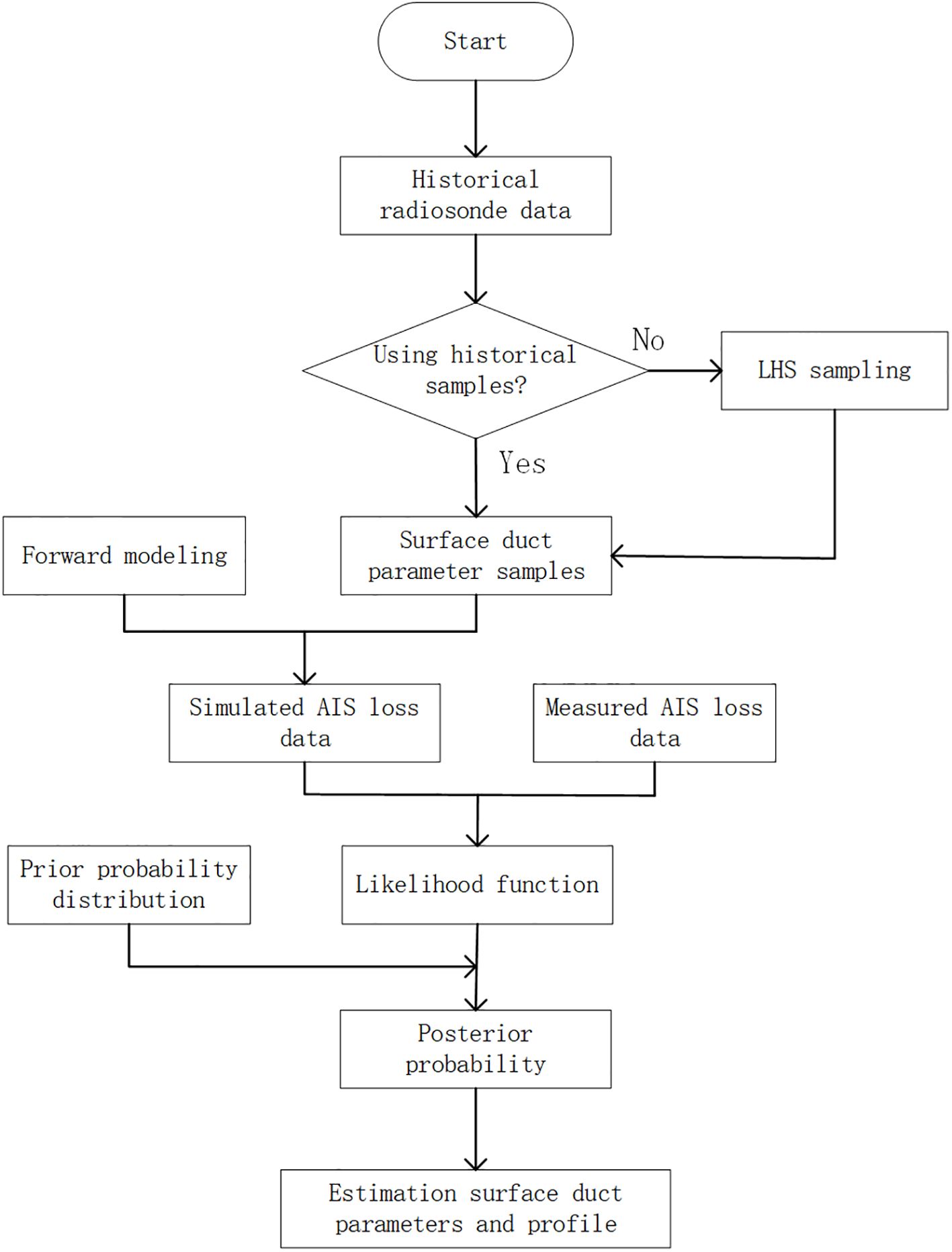
Figure 5. Flowchart of the inversion process.

3.1 AIS observation data

The raw data received by AIS contains the received power and the latitude/longitude of the radiation source. By combining the AIS transmission and reception parameters, the AIS path loss at different distances can be calculated as follows (Zhang et al., 2022):

$\begin{array}{ll}{L}^{obs}=P_t+G_t-L_t+G_r-L_r-P_r& (7)\end{array}$

where P_t is transmitter power, G_t is transmitter antenna gain, L_t is transmitter cable loss, G_r, L_r, and P_r is receiver antenna gain, cable loss, and receiver power, respectively. The typical transmitter and receiver parameters of AIS are shown in Table 2.

Table 2

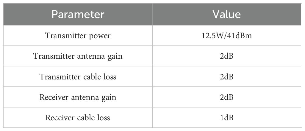
Table 2. Typical parameters of the AIS transmitter and receiver.

3.2 Computing the likelihood function

The likelihood function describes the probability of observing the current data given the model parameters, measuring the degree of match between the model parameter values and the observed data. The larger the value of the likelihood function, the greater the probability of the observed data occurring under the current parameters. It can be considered that the AIS observation error follows a Gaussian distribution, then the likelihood function takes the form of a Gaussian probability density function, which is a function of the error between the AIS simulated path loss and the AIS observation data, expressed as:

$\begin{array}{ll}p(err)=\frac{1}{\sqrt{2\pi }\sigma }{e}^{-\frac{er{r}^2}{2{\sigma }^2}}& (8)\end{array}$

where err is the error, σ is the observation standard deviation. The error is:

$\begin{array}{ll}err=\sqrt{e^{T}e}& (9)\end{array}$

where $e=L^{obs}-L^{sim}-({\overline{L}}^{obs}-{\overline{L}}^{sim})$, L^obs is the observed path loss value, L^sim is the simulated path loss value based on the sampled surface duct parameters, ${\overline{L}}^{obs}$ and ${\overline{L}}^{sim}$ are the average values of observed and simulated path loss respectively.

3.2.1 Latin hypercube sampling of surface duct parameters

Based on the probability density function of surface duct parameters fitted in Table 1, Latin hypercube sampling was used to obtain samples of surface duct parameters. Latin hypercube sampling is a method for approximately random sampling from multivariate parameter distributions, belonging to stratified sampling techniques (Han et al., 2022a). For each surface duct parameter, uniformly partition its spatial domain into N mutually non-overlapping sub-spaces, and randomly select one point within each sub-space, as shown in Figure 6. Sample each dimension as described above, then randomly permute and combine the sampling points from different dimensions to form a multidimensional sampling point matrix. The surface duct parameters obtained through Latin hypercube sampling are mutually independent. To obtain sampling data that better aligns with the actual distribution, the rank correlation method is employed for the elevated-surface duct to account for the correlation among atmospheric duct parameters. The correlation coefficient between the LHS-generated duct height and duct intensity of the SBD is -0.047. The correlation coefficient matrix of the LHS-generated ESD parameters is:

Figure 6

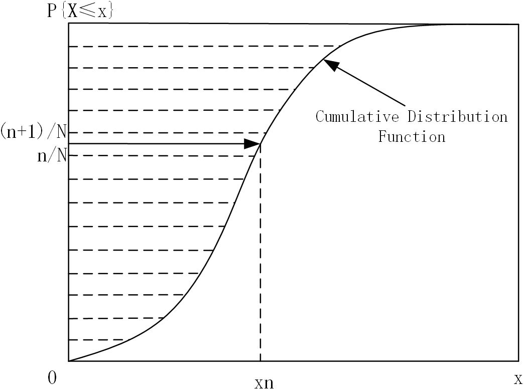
Figure 6. Schematic diagram of LHS.

$\begin{array}{ll}{\rho }_{\text{LHS-ESD}}=\left[\begin{array}{ccc}1& 0.585& 0.802\\ 0.585& 1& 0.579\\ 0.802& 0.579& 1\end{array}\right]& (10)\end{array}$

Comparing Equation 10 and Equation 5, it can be observed that the correlation coefficients of the surface duct parameters generated by LHS-generation are consistent with historical statistical data.

3.2.2 Simulation of AIS path loss in surface duct environments

The forward model adopts the parabolic equation (PE) method to achieve simulation calculations of AIS path loss in surface duct environments. The PE is an approximation of the wave equation, used to simulate the propagation of electromagnetic energy within a conical region (near-axis direction) in a given orientation. For the issue of electromagnetic wave propagation in ducting environments, the PE obtained via the paraxial approximation is sufficiently accurate and can be algorithmically implemented using FFT, achieving outstanding computational efficiency advantages. The form of PE is (Levy, 2000; Sirkova, 2006; Han et al., 2022a):

$\begin{array}{ll}\frac{{\partial }^{2}u(x,z)}{\partial z^2}+2ik\frac{\partial u(x,z)}{\partial x}+k^2(n^2(x,z)-1+\frac{2z}{a_e})=0& (11)\end{array}$

where u(x, z) is the electromagnetic field component at range x and height z in Cartesian coordinates, k is the wave number in free-space, $n=1+(M-0.157z)/{10}^6$ is the refractive index, and a is the radius of the Earth.

PE can be solved using the split-step Fourier algorithm, expressed as:

$\begin{array}{ll}u(x+\Delta x,z)=e^{\frac{ik(n^2(x,z)-1+\frac{2z}{a_e})}{2}}{\Im }^{-1}(e^{\frac{-i{\pi }^2{p}^2\Delta x}{2}}\Im u(x,z))=0& (12)\end{array}$

where ${\Im }^{-1}$ are $\Im$ Fourier transform and inverse transform respectively, p is the transform variable. The solution at $x+\Delta x$ in terms of the solution at x0 is implemented numerically using the split-step Fourier algorithm. As indicated in (11), one must start with an initial field to propagate the field forward. This initial field is generated by the Fourier transform relationship between the aperture distribution and the radiation pattern of an antenna. The path loss is expressed in dB as (Han et al., 2022b):

$\begin{array}{ll}{L}^{sim}=20\log f+10\log (R)-20\log \left|u\right|-27.6& (13)\end{array}$

where f is the AIS signal frequency, R is the distance from the point in the PE region to the position of the AIS receiver.

4 Inversion and analysis

The inversion of surface ducts is performed using shore-based AIS measured data. The AIS receiver is located at Chengshantou along the coast of China’s Yellow Sea, continuously receiving signals from maritime shipborne AIS radiation sources. The AIS receiving antenna has a height of 15m, corresponding to a radio horizon of approximately 40km, which means the maximum distance for receiving radiation sources under normal atmospheric refraction conditions is around 40km. The receiver obtains the received power and message data by demodulating and decoding the AIS signal, and the position of the AIS emitter can be parsed from the message. The AIS reception data on April 20 is shown in Figure 7, with the farthest reception distance in the southeast direction exceeding 300 km. This is due to the effect of the atmospheric duct, which enables AIS to achieve over-the-horizon propagation. To match the meteorological sounding release time, AIS reception data at the 135-degree azimuth from 00:00 to 00:30 UTC were selected to obtain the measured path loss, as shown in Figure 8. The measured path loss data serves as the input data for the inversion of surface duct parameters. This study conducts Bayesian inversion based on historical surface duct data samples and LHS sampling samples, respectively.

Figure 7

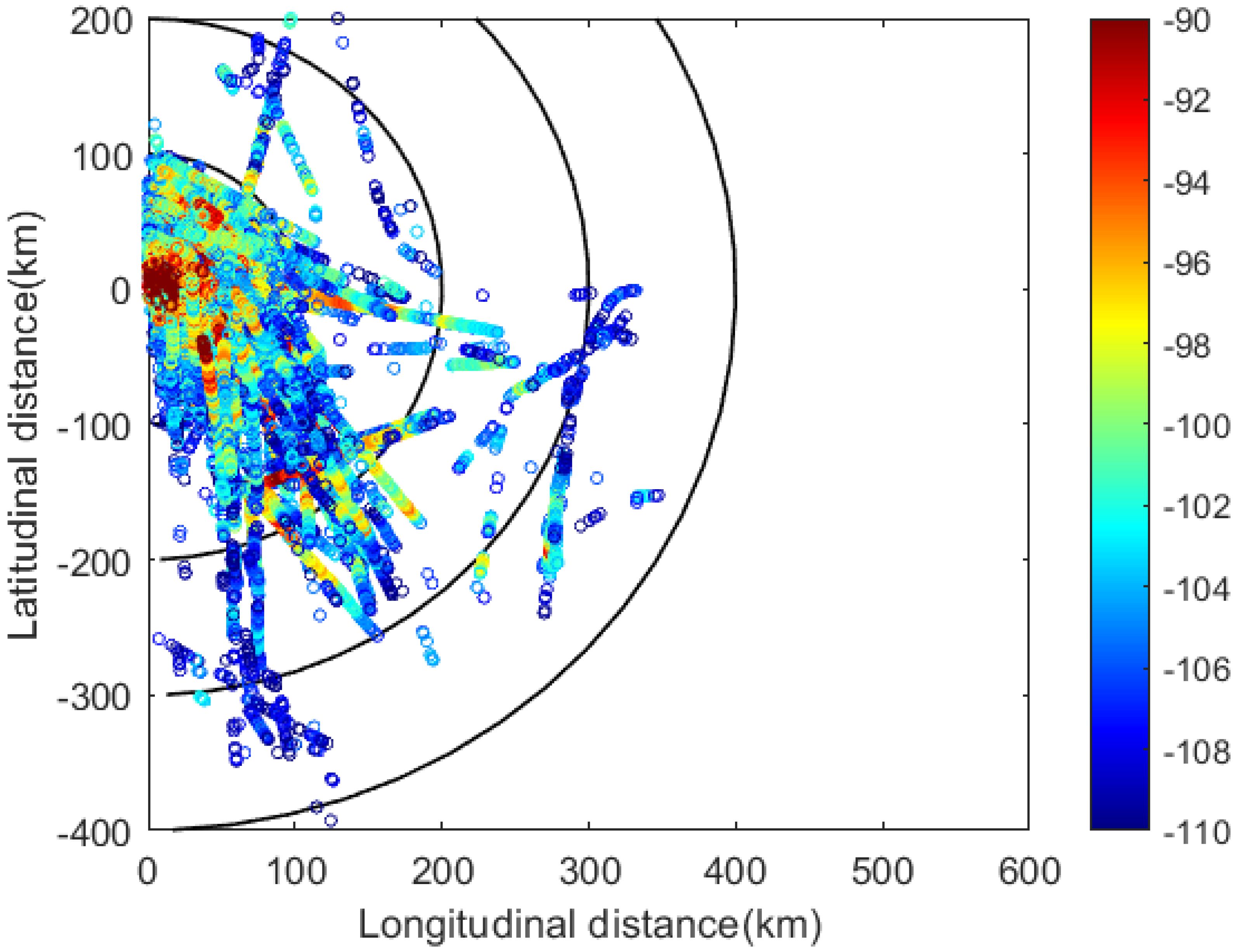
Figure 7. AIS received the power and radiation source location.

Figure 8

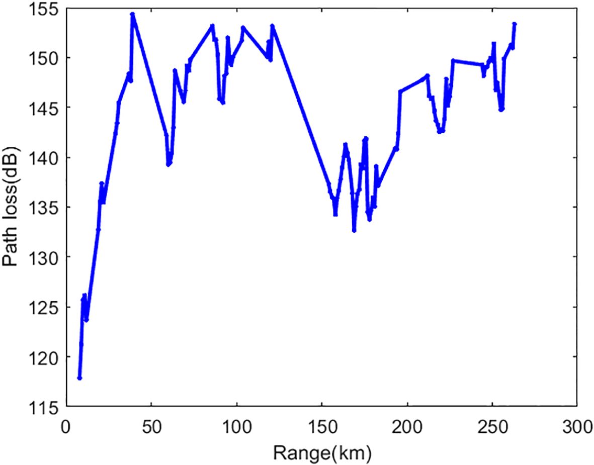
Figure 8. Measured path loss varies with distance.

4.1 Inversion based on historical data as samples of surface ducts

First, directly using 16,138 historical data samples as prior information, the surface duct parameters are inverted based on the Bayesian inference method by utilizing measured path loss data. No distinction is made between surface-based duct and elevated-surface duct. Calculate the path loss using the forward model simulation, and obtain the likelihood function based on the difference between the measured and simulated path losses. Figure 9 displays the results of the likelihood function. Since both the surface-based duct and the elevated-surface duct contain the surface duct height and surface duct intensity, the joint probability density of the surface duct height and intensity, i.e., the prior probability, can be obtained based on historical data samples. Multiplying this by the likelihood function yields the posterior probability, as shown in Figure 10. The surface duct parameters for the final inversion are obtained based on the maximum a posteriori probability. Figure 11 presents the modified refractivity profile of the surface duct derived from the inversion parameters of the surface duct. The result shows a surface duct with a base layer, where the height, intensity, and base height of the surface duct are 282.4m, 9.3 M-units, and70.9m, respectively. Based on the posterior probability, the marginal probability distributions of the surface duct height and intensity can also be obtained.

Figure 9

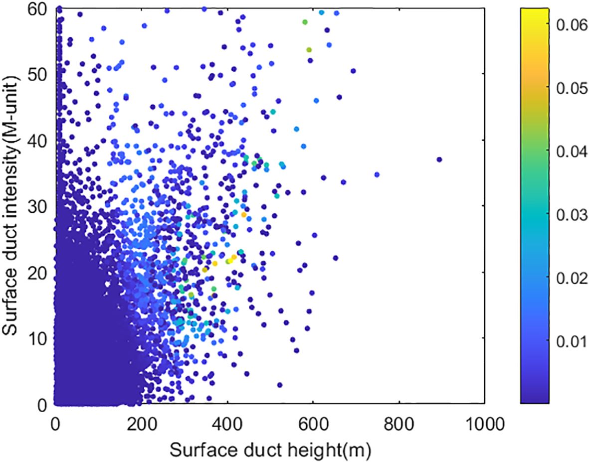
Figure 9. Likelihood function results.

Figure 10

Figure 10. Posterior probability results.

Figure 11

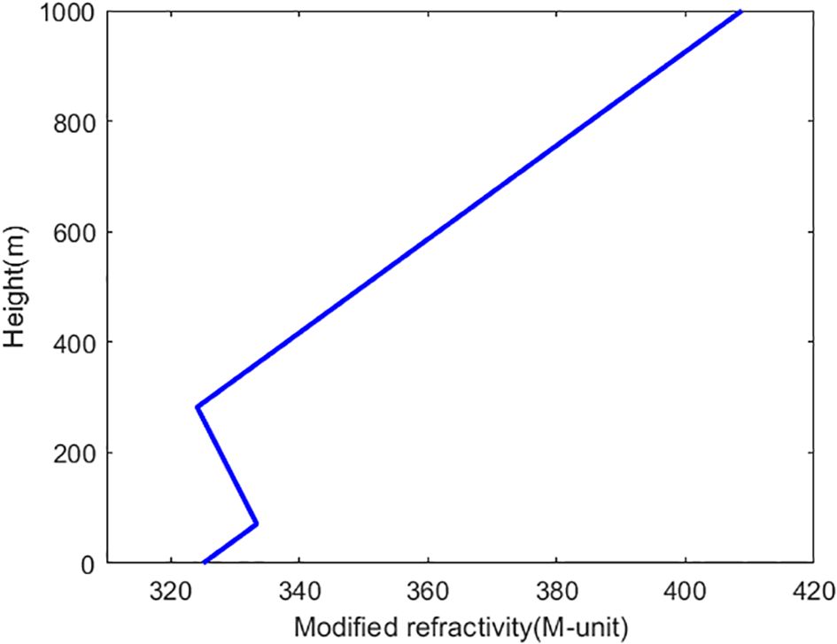
Figure 11. Surface duct profile inversion results.

4.2 Inversion based on LHS sampling results

Next, using the fitted probability density function of surface duct parameters from Section 2.2 as the prior probability, the inversion of surface duct parameters is performed by distinguishing between surface-based ducts and elevated-surface ducts. Sampling values of surface-based ducts and elevated-surface ducts were obtained using the LHS method respectively. Here, the number of samples generated by LHS is kept at the same order of magnitude as the historical data samples, with the sample size for surface-based duct parameters being 10,000 and that for elevated-surface duct parameters being 2,900. Figure 12 shows the probability density distribution of the duct height parameter for the surface-based duct and the histogram of the LHS-generated data.

Figure 12

Figure 12. Histogram of the LHS-generated duct height data.

Similarly, the forward model is utilized to calculate the simulated path loss, which is then combined with the measured path loss to derive the likelihood functions for the two types of surface ducts. These are multiplied by the prior probabilities to obtain the posterior probabilities. Figure 13 presents the posterior probability results of the two types of surface ducts. Based on maximum a posteriori probability, the surface-based inversion results for duct height and intensity are 99.2m and 3.7 M-unit, respectively. The inversion results for the duct height, intensity, and base height of the elevated-surface duct are 334.5m, 17.2 M-unit, and 52.0m, respectively. Figure 14 depicts the modified refractivity profiles of the two types of surface duct, derived from the estimation parameters of the surface duct. The marginal probability distributions of the elevated-surface duct height, intensity, and base height are obtained based on the posterior probability, as shown in Figure 15.

Figure 13

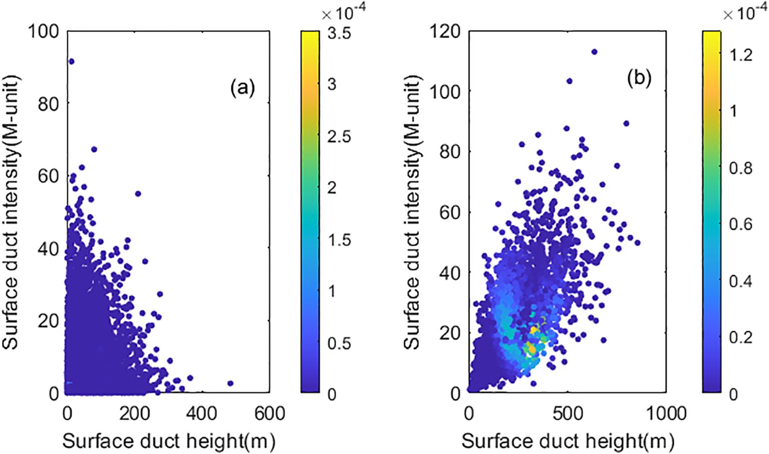
Figure 13. Posterior probability results based on LHS samples. (a) Surface-based ducts; (b) Elevated-surface ducts.

Figure 14

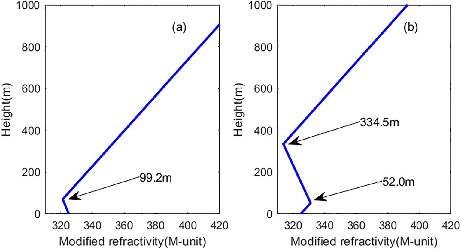
Figure 14. Two types of surface duct profile inversion results. (a) Surface-based ducts; (b) Elevated-surface ducts.

Figure 15

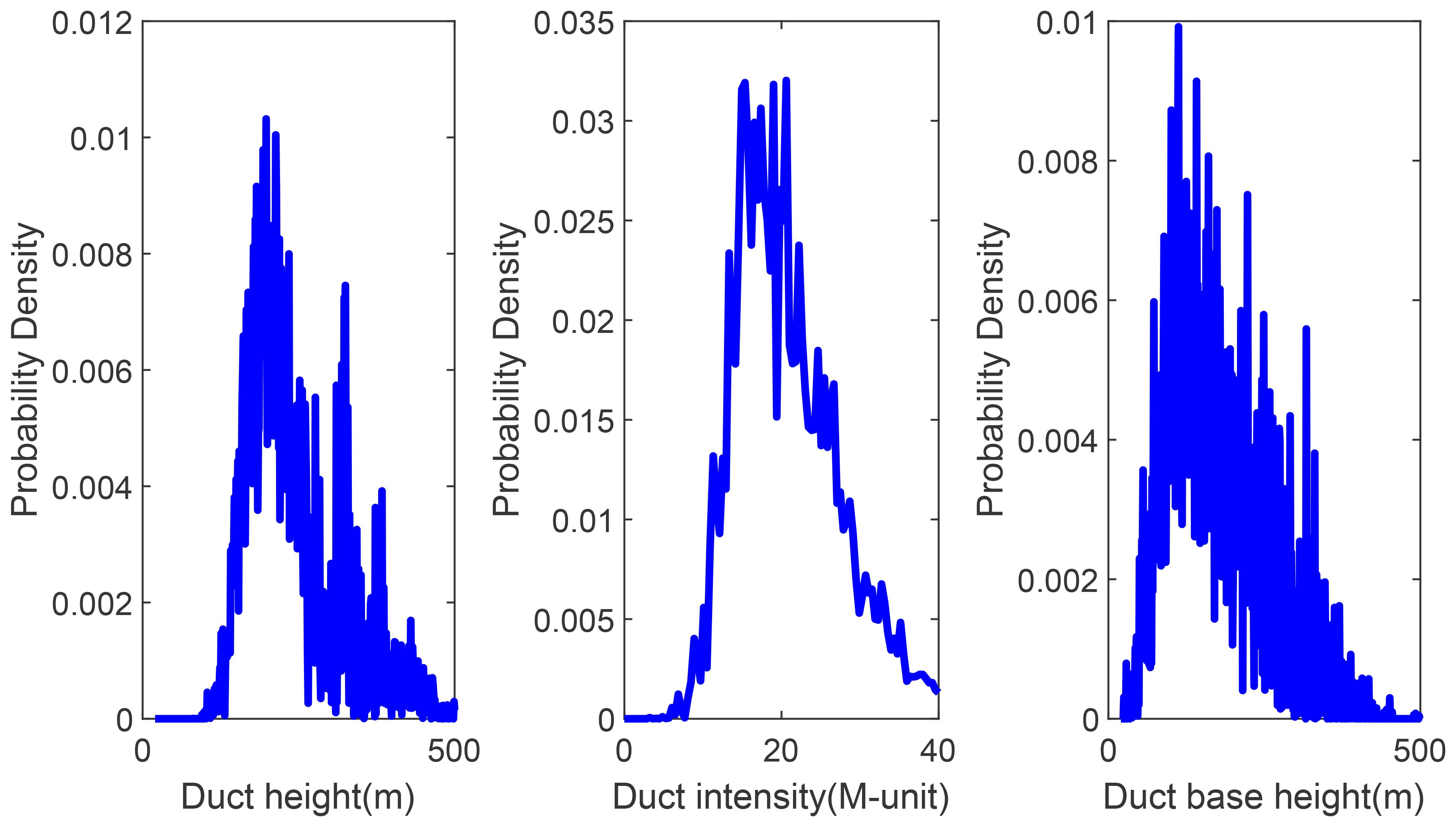
Figure 15. Marginal probability distributions of the elevated-surface duct parameters.

4.3 Comparison and analysis

Based on the surface duct profiles inverted in Sections 4.1 and 4.2, the AIS path loss was calculated using the forward model and compared with the measured path loss to analyze the accuracy of the inversion results. The better the consistency between the model calculations and the measured results, the more accurate the corresponding surface duct inversion results. The comparison results of AIS loss are shown in Figure 16. As can be seen from the figure, the inversion results calculated from both the historical surface duct sample data and the LHS elevated-surface duct samples show good agreement with the measured loss values, while the calculated values from the LHS surface duct samples exhibit significant deviations from the measured values. Therefore, the inversion results of the elevated-surface duct type are more accurate. The inversion result based on historical surface duct sample data is an elevated-surface duct. Therefore, the inversion results of the elevated-surface duct type are more accurate.

Figure 16

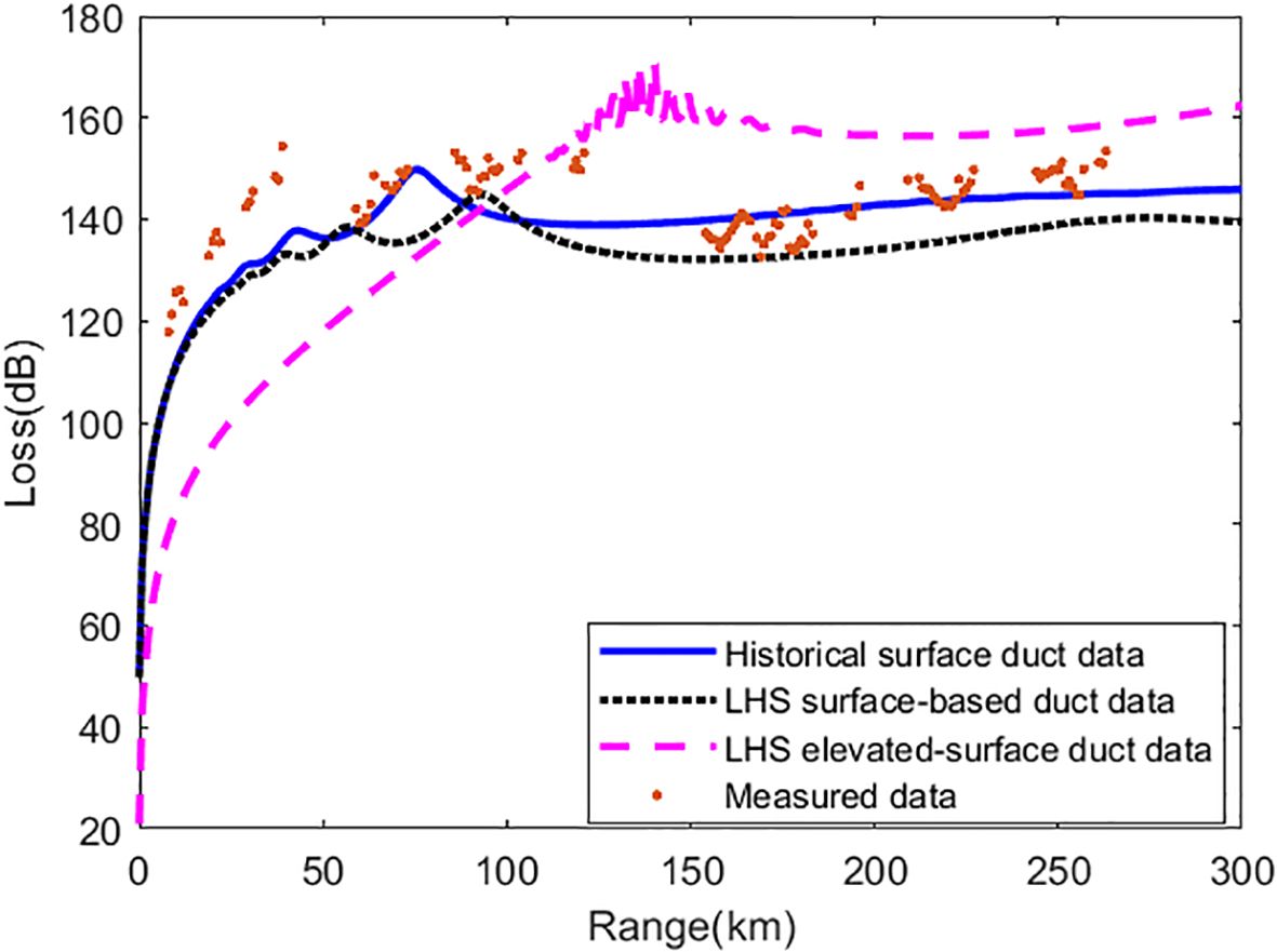
Figure 16. The comparison results of the AIS loss.

According to Equation 9, the error between the model calculation and the measured AIS path loss is obtained, which can quantitatively compare the accuracy of the inversion results. The error can serve as an evaluation indicator, illustrating the effectiveness of the method. The smaller the error, the more accurate the inversion result. The inversion parameters and error results are shown in Table 3. The results indicate that the inversion of elevated-surface duct based on LHS-sampled data is the most accurate, and the elevated-surface duct inversion results obtained from historical data are also relatively accurate.

Table 3

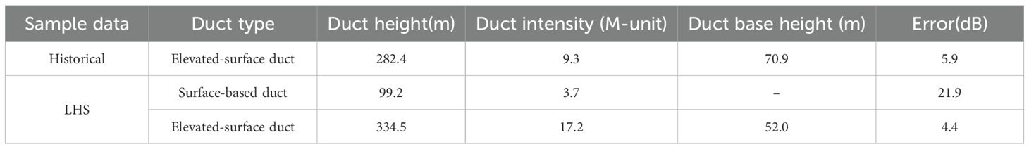
Table 3. The inversion parameters and error results.

Reference (Huang et al., 2023) utilizes intelligent optimization algorithms for atmospheric duct inversion using AIS signals. The algorithms specifically compared and analyzed are the genetic algorithm, simulated annealing, and particle swarm optimization (PSO). The results indicated that the PSO algorithm exhibited the best inversion performance. The advantage of the Bayesian algorithm used in this paper does not stem from its precision; rather, it lies in its capacity to perform forward calculations proactively, with a rapid inversion process, and to yield the probability distribution of the inversion parameters.

5 Discussion

Marine atmospheric duct environmental information is primarily obtained through the inversion of various radio signals. Currently, the main inversion algorithms for atmospheric ducts are global optimization algorithms, followed by machine learning methods. Compared to the aforementioned methods, the approach proposed in this paper, which utilizes AIS received data and is based on Bayesian inversion of marine atmospheric duct parameters, possesses distinct advantages: (1) In addition to obtaining parameter inversion results, it also provides the benefit of deriving their probability distributions; (2) It makes more comprehensive use of prior information; (3) It enables the pre-calculation of simulation results by leveraging PE and sampled data in advance, thereby overcoming the drawback of slow inversion speed associated with global optimization algorithms. The results of this paper demonstrate that this method can directly utilize historical statistical samples, with its maximum a posteriori probability inversion results being physically existing and credible surface duct parameters; it can also employ random samples, yielding more accurate inversion results.

Data availability statement

The original contributions presented in the study are included in the article/supplementary material. Further inquiries can be directed to the corresponding author.

Author contributions

H-GW: Conceptualization, Investigation, Methodology, Resources, Validation, Writing – original draft, Writing – review & editing. L-JZ: Data curation, Formal analysis, Investigation, Methodology, Project administration, Software, Supervision, Visualization, Writing – review & editing. JH: Data curation, Methodology, Writing – review & editing. L-FH: Investigation, Software, Visualization, Writing – review & editing. Q-LZ: Conceptualization, Project administration, Resources, Supervision, Validation, Writing – original draft, Writing – review & editing.

Funding

The author(s) declare that no financial support was received for the research and/or publication of this article.

Conflict of interest

The authors declare that the research was conducted in the absence of any commercial or financial relationships that could be construed as a potential conflict of interest.

Generative AI statement

The author(s) declare that no Generative AI was used in the creation of this manuscript.

Publisher’s note

All claims expressed in this article are solely those of the authors and do not necessarily represent those of their affiliated organizations, or those of the publisher, the editors and the reviewers. Any product that may be evaluated in this article, or claim that may be made by its manufacturer, is not guaranteed or endorsed by the publisher.

References

Bruin E. R. (2016). On propagation effects in Maritime Situation Awareness: modelling the impact of North Sea weather conditions on the performance of AIS and coastal radar systems (Master's thesis). Utrecht University.

Google Scholar

Compaleo J., Yardim C., Xu L., Wijesundara S., Johnson J., Burkholder B., et al. (2018). Preliminary refractivity from clutter (RFC) evaporation duct inversion results from CASPER west experiment[C]//2018 IEEE Radar Conference (RadarConf18). IEEE . p, 1516–1521. doi: 10.1109/RADAR.2018.8378791

Crossref Full Text | Google Scholar

Douvenot R., Fabbro V., Gerstoft P., and Bourlier C and Saillard J. (2010). Real time refractivity from clutter using a best fit approach improved with physical information. Radio Sci. 45, 1–13. doi: 10.1029/2009RS004137

Crossref Full Text | Google Scholar

Gerstoft P., Rogers L. T., Krolik J. L., and Hodgkiss W. S. (2003). Inversion for refractivity parameters from radar sea clutter. Radio Sci. 38, 8053. doi: 10.1029/2002RS002640

Crossref Full Text | Google Scholar

Guo X. M., Li Q. L., Zhao Q., Kang S. F., Wei Y. W., and Yang L. X. (2023). A comparative study of rough sea surface and evaporation duct models on radio wave propagation. IEEE Trans. Antennas Propagation. 71, 6060–6071. doi: 10.1109/TAP.2023.3276571

Crossref Full Text | Google Scholar

Han J., Wu J. J., Wang H. G., Zhu Q. L., Zhang L. J., Zhang C., et al. (2022a). Weight loss function for the cooperative inversion of atmospheric duct parameters. Atmosphere 13, 338. doi: 10.3390/atmos13020338

Crossref Full Text | Google Scholar

Han J., Wu J. J., Zhang L. J., Wang H. G., Zhu Q. L., Zhang C., et al. (2022b). A classifying-inversion method of offshore atmospheric duct parameters using AIS data based on artificial intelligence. Remote Sens. 14, 3197. doi: 10.3390/rs14133197

Crossref Full Text | Google Scholar

Hao X. J., QL L. I., Huo L. X., and Lin L. K. (2022). Digital maps of atmospheric refractivity and atmospheric ducts based on a meteorological observation datasets. IEEE Trans. Antennas Propag. 70, 2873–2883. doi: 10.1109/TAP.2021.3098582

Crossref Full Text | Google Scholar

Huang L. F., Liu C. G., Wu Z. P., Zhang L. J., Wang H. G., Zhu Q. L., et al. (2023). Comparative analysis of intelligent optimization algorithms for atmospheric duct inversion using automatic identification system signals. Remote Sens. 15, 3577. doi: 10.3390/rs15143577

Crossref Full Text | Google Scholar

ITU-R M.1371-5 (2014). Technical Characteristics for an Automatic Identification System Using Time-Division Multiple Access in the VHF Maritime Mobile Frequency Band Vol. 9 (Geneva, Switzerland: International Telecommunication Union (ITU).

Google Scholar

ITU-R M.2123 (2007). Long Range Detection of Automatic Identification System (AIS) Messages Under Various Tropospheric Propagation Conditions (Geneva, Switzerland: International Telecommunication Union (ITU).

Google Scholar

ITU-R P.310-10 (2019). Definitions of terms relating to propagation in non-ionized media (Geneva: International Telecommunications Union).

Google Scholar

ITU-R P.453-10 (2012). The radio refractive index: its formula and refractivity data (Geneva: International Telecommunications Union).

Google Scholar

Kang S. F., Cao Z. Q., and Li J. R. (2017). Information assurance technology for radio environment of radio equipment over sea. Equip. Environ. Engineering. 14, 1–6.

Google Scholar

Karimian A., Yardim C., Gerstoft P., Hodgkiss W. S., and Barrios A. E. (2011). Refractivity estimation from sea clutter: An invited review. Radio Sci. 46, 1–16. doi: 10.1029/2011RS004818

Crossref Full Text | Google Scholar

Levy M. F. (2000). Parabolic Equation Methods for Electromagnetic Wave Propagation (London, UK: The Institution of Electrical Engineers).

Google Scholar

Liao Q., Sheng Z., Shi H., Xiang J., and Yu H. (2018). Estimation of surface duct using ground-based GPS phase delay and propagation loss. Remote Sens. 10, 724. doi: 10.3390/rs10050724

Crossref Full Text | Google Scholar

Lowry A. R., Rocken C., Sokolovskiy S. V., and Anderson K. D. (2002). Vertical profiling of atmospheric refractivity from ground-based GPS. Radio Sci. 37, 1–21. doi: 10.1029/2000RS002565

Crossref Full Text | Google Scholar

Mentes S. and Kaymaz Z. (2007). Investigation of surface duct conditions over Istanbul, Turkey. J. Appl. meteorology climatology. 46, 3. doi: 10.1175/JAM2452.1

Crossref Full Text | Google Scholar

Sirkova I. (2022) “Automatic Identification System Signals propagation in troposphere ducting conditions,” in In Proceedings of the IEEE International Black Sea Conference on Communications and Networking (BlackSeaCom), Sofia, Bulgaria, 331–335. doi: 10.1109/BlackSeaCom54372.2022.9858131

Crossref Full Text | Google Scholar

Sirkova I. (2023). Revisiting enhanced AIS detection range under anomalous propagation conditions. J. Mar. Sci. Eng. 11, 1838. doi: 10.3390/jmse11091838

Crossref Full Text | Google Scholar

Sirkova I. and Mikhalev M. (2006). Parabolic wave equation method applied to the tropospheric ducting propagation problem: A survey. Electromagnetics 26, 155–173. doi: 10.1080/02726340500486484

Crossref Full Text | Google Scholar

Tang W. L., Cha H., Wei M., and Tian B. (2019). Estimation of surface-based duct parameters from automatic identification system using the Levy flight quantum-behaved particle swarm optimization algorithm. J. Electromagnetic Waves Applications. 33, 827–837. doi: 10.1080/09205071.2018.1560365

Crossref Full Text | Google Scholar

Wang H. G., Wu Z. S., Kang S. F., and Zhao Z. W. (2013). Monitoring the marine atmospheric refractivity profiles by ground-based GPS occultation. IEEE Geosci. Remote Sens. 10, 962–965. doi: 10.1109/LGRS.2012.2227294

Crossref Full Text | Google Scholar

Yang C., Shi Y. F., Wang J., and Feng F. (2022a). Regional spatiotemporal statistical database of evaporation ducts over the south China sea for future long-range radio application. IEEE J. Selected Topics Appl. Earth Observations Remote Sensing. 15, 6432–6444. doi: 10.1109/JSTARS.2022.3197406

Crossref Full Text | Google Scholar

Yang C., Wang J., and Shi Y. F. (2022b). A multi-dimensional deep-learning-based evaporation duct height prediction model derived from MAGIC data. Remote Sensing 14, 5484. doi: 10.3390/rs14215484

Crossref Full Text | Google Scholar

Yardim C., Gerstoft P., and Hodgkiss W. S. (2006). Estimation of radio refractivity from radar clutter using Bayesian Monte Carlo analysis. IEEE Trans. Antennas Propag. 54, 1318–1327. doi: 10.1109/TAP.2006.872673

Crossref Full Text | Google Scholar

Zhang L. J., Wang H. G., and Li J. R. (2022). Experimental analysis of low atmospheric duct monitoring based on AIS signal. Chin. J. Radio Sci. 38, 108–113. doi: 10.12265/j.cjors.2021339

Crossref Full Text | Google Scholar