Abstract
Vertical migration is a rather complex behavior by which multiple species of different sizes move from the meso- and bathy-pelagic zones, where they reside during day to avoid predators, to the epipelagic zone for feeding. Understanding this behavior of zooplankton organisms is key to assess their role in the active transport of carbon in the oceans. The present study disentangles the diel vertical distribution of zooplankton community (mainly copepods) during spring in the Northeast Atlantic Ocean. To address that, 10 stations down to 1900 m depth were sampled using an opening-closing MOCNESS during day- and nighttime. Additionally, we also sampled the epipelagic strata (0–200 m) for microzooplankton (50-200 µm) as well as the mesozooplankton community (>200 µm). A total of 15 zooplankton groups were found (>85% were copepods), and more than 250 species of copepods were identified. The results showed a latitudinal decreasing gradient northward in the number of genera and species, and an increasing gradient in their abundances. A frontal system was observed in the epipelagic layer between 45° and 47°N promoting sharp differences among the northern and southern communities. In this frontal zone, small copepod nauplii and copepodites were rather abundant, being Paracalanus parvus the dominant copepod. In the most northern region, we found Calanus finmarchicus and a high abundance of Oithona spp, while in the southern region C. helgolandicus, Nannocalanus minor and Mecynocera clausi were dominant. A decreasing trend of copepod abundance was observed with depth, segregating the upper 700 m from below. Using the 50 dominant copepod species, five different groups were distinguished in their vertical distributions: (1) the non-migrant epipelagic copepods, (2) copepod migrating from mid-waters to the epipelagic zone at night, (3) copepods abundant in the epipelagic layer but performing reverse migration, (4) the strong migrants moving from the meso- and bathypelagic zones to the epipelagic zone at night, and (5) those just moving into the twilight zone. Our findings highlight the complexity of the diel vertical migration pattern of copepods during spring and their relevant role in the deep-sea of the North Atlantic Ocean.
1 Introduction
In marine food webs, copepods are essential organisms connecting primary producers with higher trophic levels, contributing significantly to the biological carbon pump (Steinberg and Landry, 2017). Through their vertical migration, copepods feed in the epipelagic layers and export organic matter to the meso- and bathypelagic zones (Hernández-León et al., 2020). Although they sharply decrease with depth, copepods are the dominant organisms of the mesozooplankton community across all oceans, playing a central role in the marine ecosystem (Bucklin et al., 2010). Copepods exhibit complex and different vertical distributions in all oceans (Cushing, 1951; Vinogradov, 1977; Roe, 1984) particularly in the tropical and subtropical realm compared to northern latitudes (Gaard et al., 2008; Yamaguchi et al., 2015; Fernández De Puelles et al., 2023). Zooplankton studies covering extensive regions of the North Atlantic Ocean are scarce (Gislason, 2003; Vinogradov, 2005) and to our records little information is given about the copepod structure of deep layers describing their vertical distribution down to bathypelagic depths. In this sense, changes in copepod community structure can affect global biogeochemical cycles (Turner, 2015). As such, identifying species displaying diel vertical migration (DVM) behavior is essential to understand the ocean´s ability to act as a carbon sink. Unfortunately, to identify copepod species is a time-consuming work under the stereomicroscope. Still traditional taxonomic studies are necessary not only for the study of biodiversity, but also to characterize the community structure for an accurate knowledge of the ocean ecosystem functioning (Hooff and Peterson, 2006; Bucklin et al., 2010; Fernández De Puelles et al., 2019).
Zooplankton distribution varies greatly in space and time (Mcgowan, 1989) and particularly in the North Atlantic, which is a highly diverse area covering different regions, strongly affected by the complex circulation there (Gaard et al., 2008). The area of the North Atlantic close to the Mid-Atlantic ridge (MAR) cross different geographical provinces (Longhurst, 2007), different water masses (Sarmiento-Lezcano et al., 2022), and hydrographic regions (Søiland et al., 2008), displaying an east-west asymmetry in the diversity patterns of plankton (Beaugrand et al., 2000).
Accordingly, although epipelagic zooplankton, in particular the copepods are rather well studied, their DVM to deep zones still poorly known (Vinogradov, 1997; Gaard et al., 2008). Mostly due to the inherent need for large oceanographic vessels and zooplankton sampling devices requiring time, hours of deployment during day and night and a lot of cost and requirement. A better knowledge of the vertical distribution and migrations of copepods as the main taxonomic group, implies to extend the sampling to the bathypelagic zones. Hernández-León et al. (2020) found a global coupling between primary production and bathypelagic zooplankton, suggesting that migrants were shunting energy and matter downward. This was observed as an increase of bathypelagic zooplankton biomass in areas of higher productivity. Thus, the knowledge of their diversity, vertical distribution, and diel migrations seems of paramount importance to understand this migrant pump and carbon flux.
The main goal of this study was to assess the spatial and vertical distribution of the zooplankton community focusing on copepods, their abundance and composition from the epipelagic layer to the meso- and bathypelagic zones (0–1900 m depth), during springtime when productivity levels are high. We covered an extensive area of the North Atlantic (20 to 55°N) under different oceanographic conditions from subtropical (warm and saline North Atlantic Central Water) to temperate latitudes (cold and less saline Modified North Atlantic Water) (Gibb et al., 2001; Sarmiento-Lezcano et al., 2022). Day and night vertical distribution were investigated in order to identify diel migration patterns from the meso- and bathy-pelagic zones to the epipelagic zone, providing insights towards a better understanding of the biological carbon pump.
2 Materials and methods
The study was conducted in a latitudinal transect at 22°W from the oceanic upwelling off Cape Blanc (Northwest Africa) at 20°N to the temperate North Atlantic Ocean at 55°N (see station positions in Supplementary Table S1 of Supplementary Material), covering more than 4000 km (Figure 1) during spring (May 28th to June 20th, 2018). Ten hydrological and zooplankton stations (St) were sampled during day- and nighttime on board the R.V. Sarmiento de Gamboa. Chlorophyll samples (Chl) were obtained using a Rosette equipped with 12 L Niskin Bottles at discrete depths in the upper 200 m depth. The Rosette was also equipped with a Sea-Bird 911plus for conductivity, temperature, and depth (CTD), a Sea-Bird 43 Dissolved Oxygen (DOx) sensor, and a Seapoint FLuorometer sensor. CTD casts were performed at the beginning of each of the ten stations from the surface to 2000 m depth. Fluorescence obtained in vertical profiles (0–200 m depth) was transformed to Chl a concentration. Chl a was measured in samples obtained from Niskin bottles filtering 500 ml of seawater through 25 mm Whatman glass fiber filters GF/F and freezing it at -20°C until their analysis (Hernández-León et al., 2020). Vertical profiles of temperature (T), salinity (S), density, and fluorescence (F) were averaged every 1dBar and visualized with Ocean Data view software (Schlitzer, 2022).
Figure 1
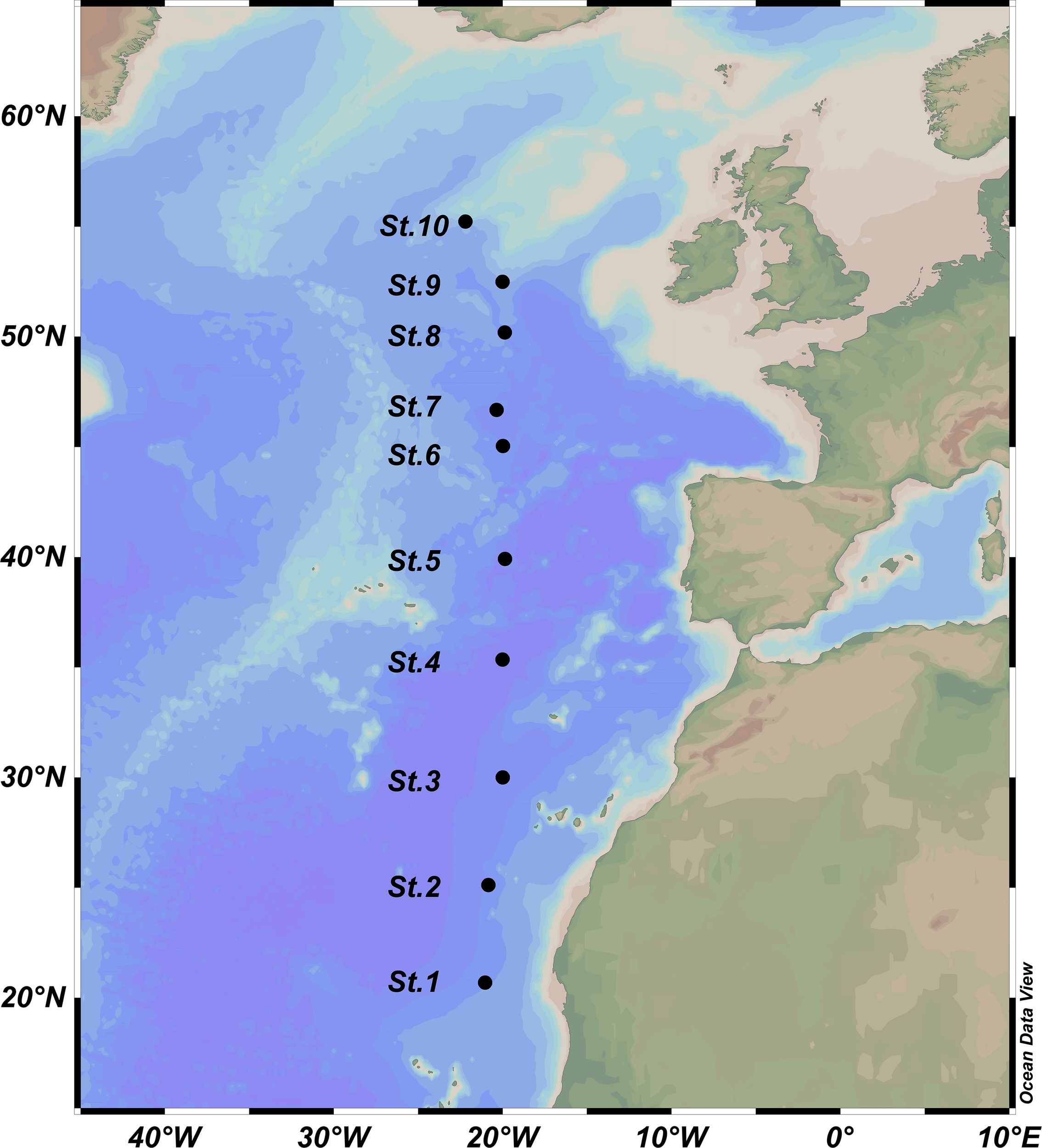
Map of the area and location of the 10 sampled stations along the 22°W transect in the North Atlantic Ocean.
Simultaneously, zooplankton samples were collected in vertical hauls during daytime from 200 m depth to the surface using a Calvet net of 53 µm mesh size to collect the smaller organisms of the zooplankton community (hereafter defined as microzooplankton). In the same frame, a double WP-2 (50 cm wide) net equipped with 200 µm mesh size for mesozooplankton (UNESCO, 1968) was also deployed. The vertical distribution of zooplankton was assessed using a MOCNESS 1m2 net (Wiebe et al., 1985) from the surface to 1900 m depth during day- and nighttime in 8 discrete strata (0-100; 100-200; 200-400; 400-700; 700-1000; 1000-1300; 1300-1600; 1600-1900). The ship speed during deployment and retrieval was maintained at 2 knots to obtain a net angle between 40 and 50°, being the winch retrieval rate fixed at 0.3 m·s-1. The volume of water filtered by each net was measured using an electronic flowmeter. Due to rough weather conditions at stations 7, 8, and 9, it was not possible to sample with the MOCNESS net, except in station 7 which was only deployed down to 700 m depth. However, we were able to collect samples with the Calvet and WP-2 nets in vertical hauls in the upper 200 m depths. Also, technical problems in the opening and closing system of the MOCNESS net precluded obtaining vertical profiles in Sts. 1 and 2. Finally, a total of 148 samples were collected at the different strata and preserved with formaldehyde (4%) for later taxonomic analysis in the laboratory.
Samples from the WP-2 and Calvet nets were splitted in two aliquots, one for biomass as dry matter after removing the water on board at 60°C during 48 h (Lovegrove, 1966), while the other was preserved with formaldehyde (4%) for taxonomic analysis under the stereomicroscope following Harris (2000). For the MOCNESS biomass, usually 1/8 of the total preserved sampled was later collected in the laboratory and dried during at least 48 h in the oven at 60°C (Boltovskoy, 1981) and the data given in dry weight units (mg DW m-3). In microzooplankton samples, all individuals were counted with the exception of Protozoa due to the mesh size used was not suitable to retrieve a representative sample (Boltovskoy, 1981). Nauplii and copepods were sorted into three groups: <0.25 mm, 0.25-0.45 mm and >0.45 mm according to Fernández de Puelles et al. (1996). Most abundant mesozooplankton groups were studied and the dominant species of copepods and cladocerans were identified, whenever possible. We focused on them following specific literature for these groups (Vives and Shmeleva, 2007, 2011; Conway, 2012; Razouls et al., 2002-2025). The list of the copepod species was made according to WoRMS (https://www.marinespecies.org). All data were standardized to number of individuals (ind·m-3). To estimate copepod diversity, we calculated the Shannon´s index (Shannon and Weiver, 1964).
The Primer-7 with Permanova software package (Clarke and Gorley, 2006; Anderson et al., 2008) was used to perform all the multivariate analyses. Cluster and non-metric multidimensional scaling analysis (NMDS) were performed looking for patterns of community structure after fourth root transformed abundance data. Hierarchical clustering was performed for samples (stations and strata) based on Bray-Curtis similarities coupled with the group average linkage. Significant groups of samples were identified using the SIMPROF procedures with a significance level of 1% (Clarke et al., 2008). The similarity percentage (SIMPER) routine was applied to identify those taxa most responsible for similarities or differences among the group of samples defined by the analysis. With this information we performed Shade plots of the 50 dominant taxa (>1%) after fourth root transformed abundance data in order to reduce the bias of the very abundant species. We have used the association index as resemblance matrix for the different copepod assemblages. Coherence plots were created after standardizing the data originated by the index of association. The copepod taxa obtained on each assemblage were averaged in order to study the different vertical migration patterns.
3 Results
3.1 Hydrology
Sea-surface temperature (SST) decreased by about 10°C from the south (latitude 20°N) to the north (55°N). The main gradient of SST was found between 40°N and 47°N (Figure 2A). We found the North Atlantic Central Water (NACW) between 20 and 30°N and 40-48°N from the surface to 700 m depth (8°<T<20°C). An increasing of temperature and salinity in the mesopelagic zone was observed around 35°N coinciding with the Mediterranean Water (MW; 2.6°<T<11°C). Antarctic Intermediate Water (AIW) was also detected between 20 and 30°N at 800–1200 m depth (4°<T<8°C). Finally, North Atlantic Deep Water (NADW) was found below 1200 m depth for most stations but approaching the surface between 50 and 55°N (4°<T<1.5°C; see details in Sarmiento-Lezcano et al., 2022). Highest salinity values at the surface were found in Sts. 2 and 3 (37.1), sharply declining northward with a minimum value of 35.1 in Station 10 (Figure 2B). We also observed the Mediterranean Water (MW) at around 1000 m depth centered at 35°N, showing a Meddy because of the high salinity observed. Dissolved oxygen (DOx) increased from low to high latitudes, increasing towards the north (Figure 2C), and an oxygen minimum zone (OMZ) was found in the lowest latitude of the transect (20-25°N). This OMZ was found in Sts. 1 and 2 located between 200 and 1000 m. Chl a was highly variable (Figure 2D) and ranged from very low values at 25°N (St. 2) to the highest values observed at 47°N (St. 7). A frontal zone was observed between stations 6 and 7 in the limit between the stratified zone (surface water >14°C in the upper 50 m layer) and the mixed water column to the north. The southern oligotrophic zone was characterized by a deep chlorophyll maximum (DCM), and further north (St. 10) values were similar in the upper 50 m layer (Figure 2). Chl a was observed to reach down to 200 m depth between 40 and 47°N at the frontal zone.
Figure 2
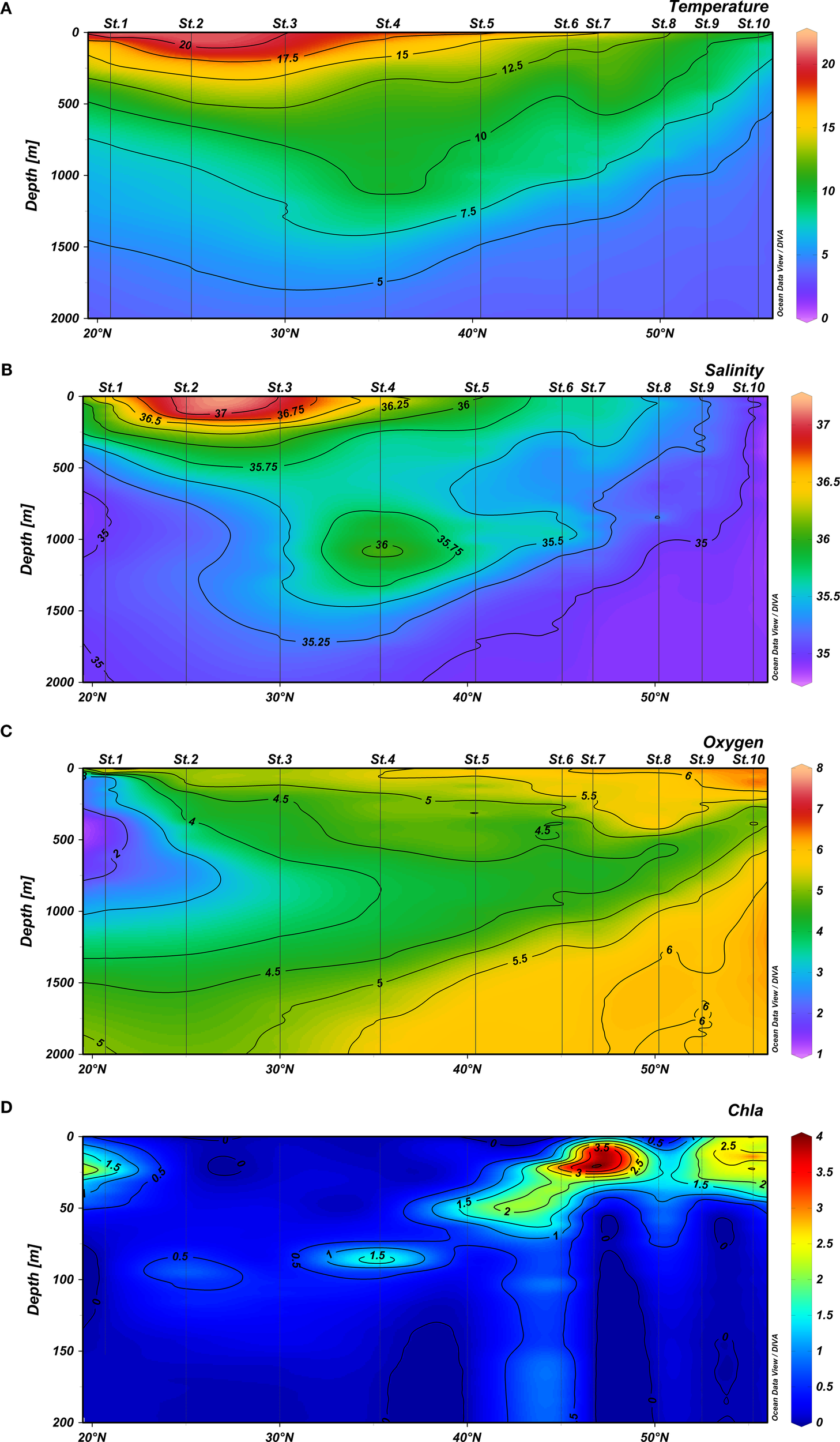
Vertical distribution (0–2000 m depth) of (A) temperature (°C), (B) salinity, (C) oxygen (ml.l-1), and (D) chlorophyll a (mg.m-3) from 0–200 m depth, along the 22°W North Atlantic Ocean studied transect.
3.2 Spatial zooplankton changes in the epipelagic layer
Across the study area, although 15 zooplankotn groups were found, 11 zooplankton groups predominated (>0.2%), with copepods being the most dominant taxa (Table 1). Copepod nauplii and copepods in the range of 100-200 µm displayed the highest abundance at the frontal zone (Sts. 6 and 7; Figure 3A). where the contribution of copepods increased to 99%. Lowest abundance values corresponded to the southern stations (south of 40°N) where the contribution of copepods was lower (86%). In the northern stations (north of 50°N), the abundance of copepods also decreased as well as the copepod contribution to the mesozooplankton community (63%, Table 1). In these northern stations, the abundance of cladocera (22%), doliolids (7%), small jellyfishes (2%), and siphonophores (2%) increased sharply (Table 1). Zooplankton biomass (Figure 3B) was low in the upper 200 m depth southwards of 45°N (microzooplankton <5 mg DW·m-3 and mesozooplankton <10 mg DW·m-3). Both size classes increased northward declining in the northernmost station. The larger community (>200 µm) showed the highest biomass in St. 9 (>40 mgDW·m-3).
Table 1
| Mesozooplankton organisms | Stations | Stations | Stations | ||||||||
|---|---|---|---|---|---|---|---|---|---|---|---|
| 1, 2, 3, 4, 5 | 6, 7 | 8, 9, 10 | |||||||||
| ind m-3 | SD | % | ind m-3 | SD | % | ind m-3 | SD | % | |||
| Copepods | 255 | 163 | 86 | Copepods | 1488 | 609 | 99 | Copepods | 643 | 376 | 63 |
| Chaetognaths | 12 | 9 | 4 | Appendicularians | 4 | 4 | 0.3 | Doliolids | 73.6 | 123 | 7.2 |
| Evadne spinifera | 7 | 13 | 2 | Ostracods | 3 | 4 | 0.3 | E. nordmanni | 223 | 43 | 22 |
| Appendicularians | 5 | 4 | 2 | Chaetognaths | 3 | 4 | 0.2 | Jellyfish | 18 | 13 | 1.8 |
| Ostracods | 4 | 4 | 1 | Euphausiids | 2 | 2 | 0.2 | Siphonophors | 14.9 | 5 | 1.5 |
| Siphonophors | 4 | 5 | 1 | Amphipods | 1 | 1 | 0.2 | Appendicularians | 12.3 | 14 | 1.2 |
| Pteropods | 3 | 5 | 1 | Pteropods | 9.03 | 9 0 | 0.9 | ||||
| Euphausiids | 3 | 6 | 1 | Euphausiids | 8.07 | 7 0 | 0.8 | ||||
| Copepod taxa | Chaetognaths | 6.85 | 6 0 | 0.7 | |||||||
| O. tenuis | 17 | 14 | 7 | Copepod taxa | Ostracods | 5.47 | 5 0 | 0.5 | |||
| P. parvus | 17 | 24 | 7 | Paracalanus juv. | 427 | 67 | 29 | Amphipods | 4.62 | 5 0 | 0.5 |
| P. denudatus | 16 | 18 | 6 | P. parvus | 224 | 121 | 15 | Copepod taxa | |||
| Paracalanus juv. | 13 | 15 | 5 | O. similis | 128 | 32 | 9 | O. atlantica | 77 | 57 | 12 |
| O. setigera | 13 | 10 | 5 | P. denudatus | 103 | 26 | 7 | O. similis | 52 | 50 | 9 |
| C. arcuicornis | 12 | 19 | 5 | C. pergens | 56 | 59 | 4 | O. tenuis | 50 | 33 | 9 |
| F. rostrata | 10 | 10 | 4 | O. atlantica | 52 | 25 | 3 | Metridia juv. | 38 | 38 | 6 |
| O. media | 8 | 5 | 3 | Clausocalanus juv. | 40 | 49 | 3 | O. setigera | 37 | 27 | 6 |
| M. tenuicornis | 8 | 9 | 3 | O. setigera | 35 | 26 | 2 | P. parvus | 35 | 28 | 5 |
| Clausocalanus juv. | 6 | 8 | 2 | C. parapergens | 34 | 49 | 2 | C. finmarchicus | 32 | 55 | 5 |
| M. clausi | 6 | 6 | 2 | O. nana | 32 | 41 | 2 | C. styliremis | 27 | 18 | 4 |
| C. styliremis | 5 | 4 | 2 | O. tenuis | 31 | 39 | 2 | Oithona juv. | 25 | 42 | 4 |
| O. plumifera | 5 | 4 | 2 | M. norvegica | 25 | 23 | 2 | Paracalanus juv. | 25 | 29 | 4 |
| C. pergens | 5 | 7 | 2 | C. pavo | 23 | 32 | 2 | M. tenuicornis | 22 | 18 | 3 |
| N. minor | 4 | 8 | 2 | C. pergens | 20 | 13 | 3 | ||||
| L. gemina | 4 | 5 | 2 | O. media | 20 | 28 | 3 | ||||
| C. parapergens | 4 | 7 | 2 | P. denudatus | 14 | 16 | 2 | ||||
| C. vanus | 10 | 8 | 2 | ||||||||
Mesozooplankton groups and dominant copepod taxa (>2%) at the different assemblages (as ind·m-3, average, standard deviation (SD) and percentage) across the epipelagic zone (0-200m depth).
Figure 3
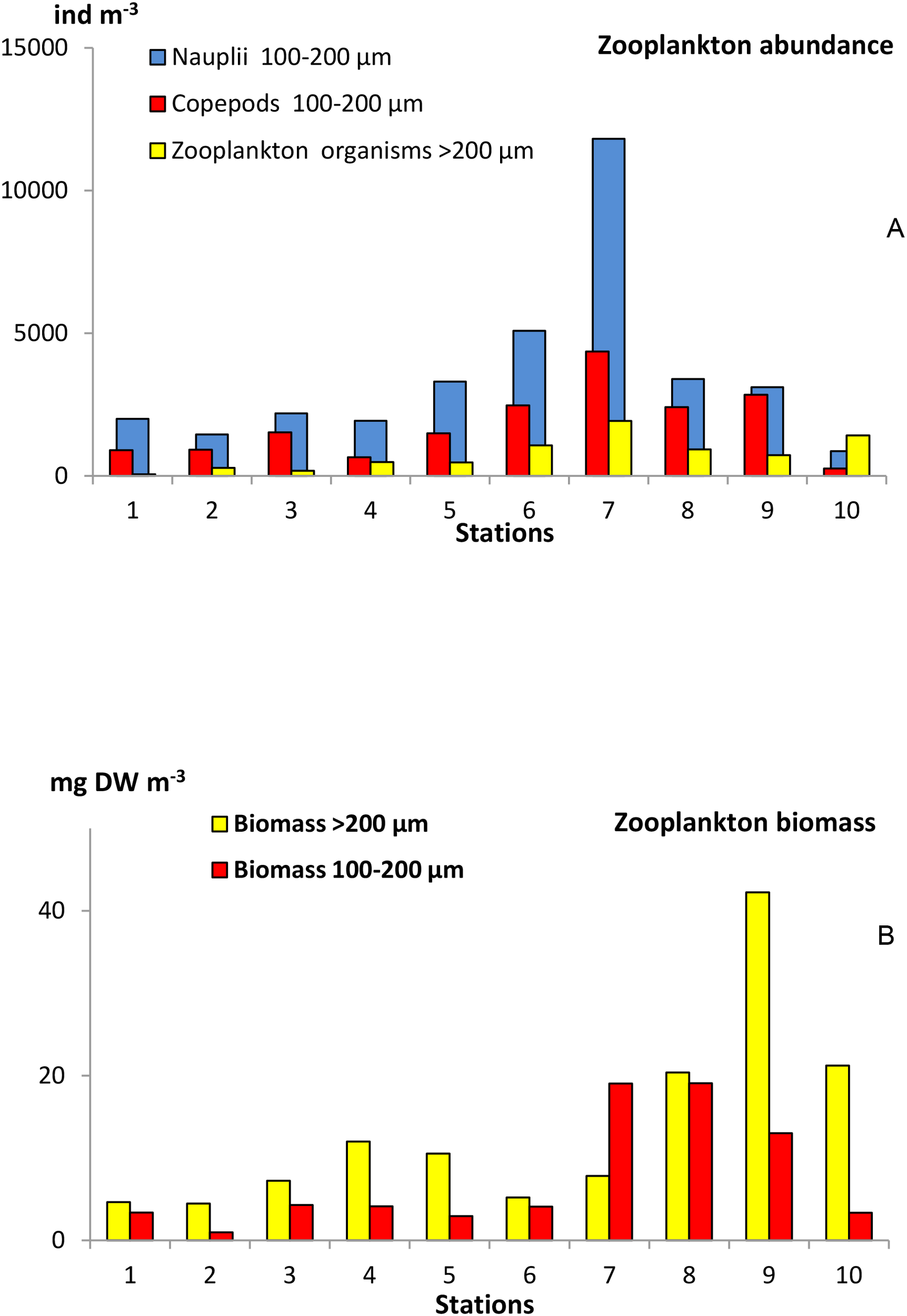
Zooplankton abundance and biomass in the epipelagic layer (0–200 m) across the studied transect. (A) Abundance (ind·m-3) of nauplii, small copepods (100-200 µm), and total zooplankton organisms (>200 µm), and (B) Biomass (mg Dry Weight·m-3) of the micro- (100-200 µm) and mesozooplankton (>200 µm) collected in the epipelagic layer (0–200 m).
Using the hierarchical clustering analysis of the total abundance of zooplankton and their dominant groups, we observed three different station assemblages (Figure 4). The first five stations in the south (similarity of 80%) were segregated from the group of Sts. 6 and 7 (similarity of 72%), coinciding with the highest gradient of temperature and salinity (82% of similarity at 45-47°N). Finally the northern stations (north of 50°N) formed by Sts. 8, 9, and 10, also showed a high similarity among them.
Figure 4
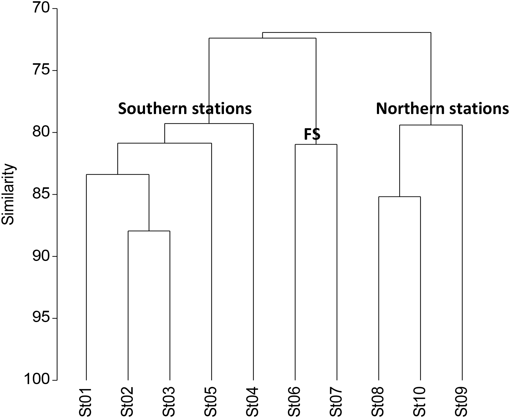
Hierarchical clustering of the sampled stations considering the abundance of the dominant taxa in the epipelagic layer (0–200 m) after fourth root transformation and a resemblance of Bray-Curtis similarity, segregating the north from the south by the frontal stations (FS).
In the upper 200 m layer, copepods were the dominant group among all zooplankton groups. We also found a gradient in richness from the southern stations (83 copepod species) to the northern stations (42 copepod species). The southern stations had less than 300 ind·m-3 while at the frontal zone (Sts. 6 and 7) the total abundance was 5 times higher. In the northern stations, the abundance decreased at least half from the frontal area. Besides the different copepods mentioned later, the cladoceran Evadne nordmanni (23%) appeared only north of 50°N.
We identified 41 genera and 95 copepod species in this layer. The dominant copepods in the whole area were Paracalanus spp. (32%), Oithona spp. (25%), and Clausocalanus spp. (10%), followed by large Calanoids. (5%), Calocalanus spp. (4%), Oncaea spp. (3%) and Metridia spp. (2%). Paracalanus spp. dominated in the frontal (Sts. 6-7) area (51%) and Oithona spp. were more relevant in the northern stations (Table 1). Paracalanus parvus was the dominant species in the frontal region (15%) although it was also present in the southern (7%) and in the northern regions (5%). However, Oithona spp. increased in the northern area (40%), being quite diversified (O. atlantica, O. similis, O. tenuis, and O. setigera). Calanus finmarchicus dominated the northern station (St. 10; 58°N) and C. helgolandicus was found further south disappearing at St. 10. Juveniles of the genus Metridia were also abundant in the northern station in the epipelagic layer as well as M. lucens. A higher number of copepod species (83) were identified in the southern stations decreasing by half in the frontal zone and further north. Hierarchical clustering of the dominant taxa (>1%) including cladocera, showed three main different assemblages in relation to the frontal region (Figure 5A). Group a (37% of similarity) was formed by species more abundant in the northern stations (E. nordmanni, C. finmarchicus, Eucalanus hyalinus, Rhincalanus nasutus, and juveniles of Metridia spp.). Group b (>50% of similarity) represented the bulk of the dominant taxa. In this group we found different species of Paracalanus, Clausocalanus, Calocalanus, Acartia, Candacia and all Corycaeidae, as well as Mesocalanus tenuicornis, Lucicutia gemina, Mecynocera clausi, Pleuromamma gracilis, and C. helgolandicus. Group c (40% of similarity) was formed by those species only found in the southern stations: Evadne spinifera, Nannocalanus minor, Oncaea venusta, Euchaeta acuta, Temora stylifera but also deeper species such as Pareucalanus sewelli or Subeucalanus subtenuis. The abundance of the dominant genera (Figure 5B) clearly showed the dominance of Paracalanus spp. in the frontal zone, while Oithona spp. dominated north of the frontal zone.
Figure 5
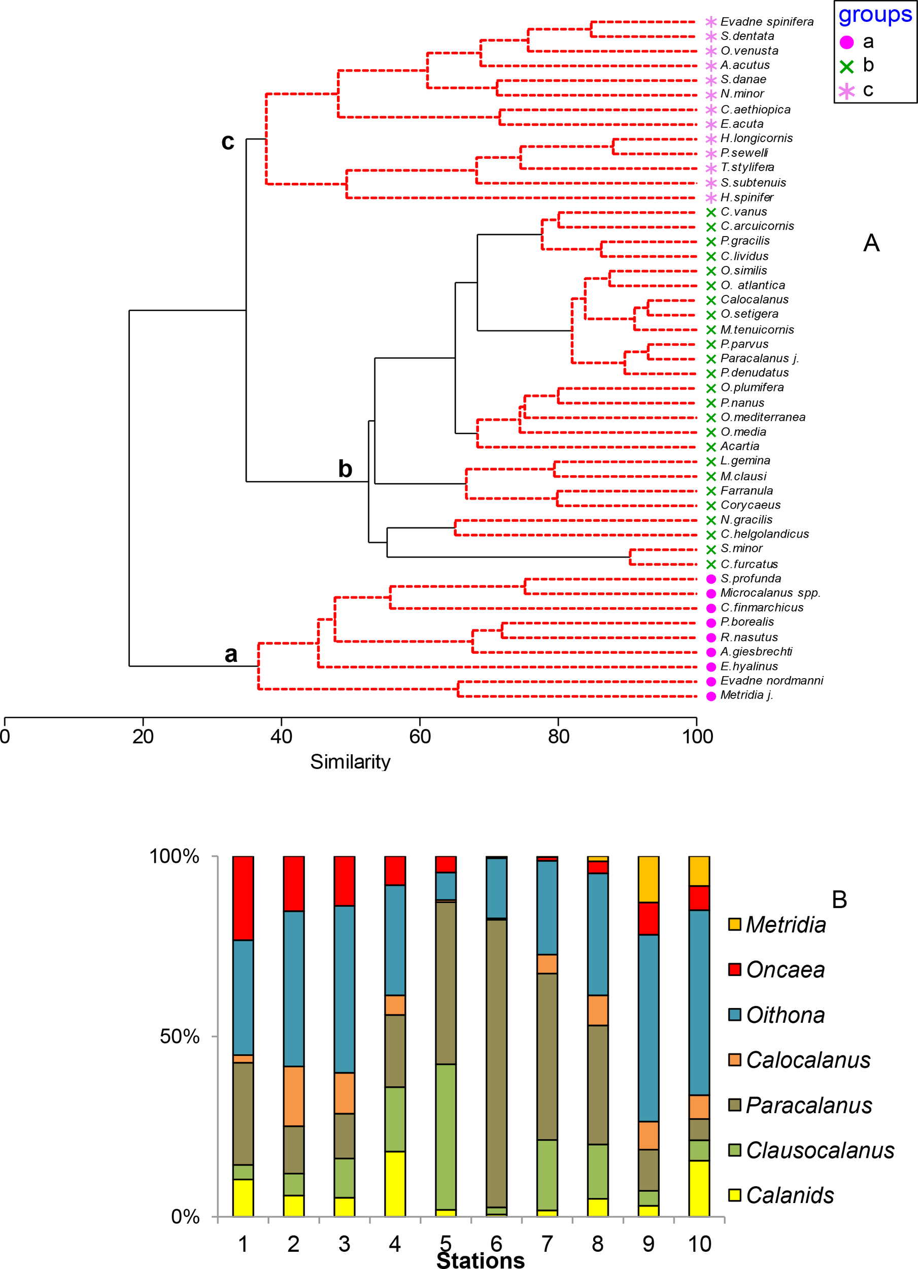
Dominant taxa (>1%) in the epipelagic layer across the transect. (A) Hierarchical clustering of the dominant copepod and cladocera taxa (ind·m-3) in the epipelagic strata indicating their presence at each area after fourth root transformation and a resemblance of Bray-Curtis similarity index and (B) dominant Copepods genera and all Calanids (%) at each station.
3.3 Vertical distribution of the dominant zooplankton groups
The vertical distribution of the dominant groups during day- and nighttime (copepods, chaetognaths, siphonophores, ostracods, and pteropods) showed a sharply decrease of abundance and biomass with depth (Figure 6). The contribution of copepods at each layer (Table 2) was usually higher than 90% with the exception at the 400–700 m layer, decreasing during daytime to 85% due to the presence of other zooplankton groups at same layer. All groups had their highest abundances in the epipelagic zone and besides copepods, very few organisms were found below 700 m depth. Ostracods were more abundant in the upper 200 m layer observing their increasing in the upper 100 m layer during night, as well as the pteropods. Siphonophores and chaetognaths showed similar abundance in the upper 100 m depth during day, although at night both seemed to be dispersed in the upper 200 m layer (Figure 6).
Figure 6

Vertical distribution of zooplankton biomass (mg·m-3) and abundance (ind·m-3) at each layer sampled from the surface to 1900 m depth by day- and nighttime (average values). The vertical profiles (ind·m-3) of copepods, chaetognaths, siphonophores, ostracods and pteropods are also shown.
Table 2
| Day | 0-100 | 100-200 | 200-400 | 400-700 | 700-1000 | 1000-1300 | 1300-1600 | 1600-1900 |
|---|---|---|---|---|---|---|---|---|
| Total zooplankton (%) | 88.9 | 6.9 | 1.8 | 1.3 | 0.5 | 0.2 | 0.2 | 0.1 |
| Copepods (%) | 89.7 | 6.5 | 1.7 | 1.2 | 0.4 | 0.2 | 0.2 | 0.1 |
| Other groups (%) | 70.1 | 18.3 | 4.2 | 5.1 | 1.1 | 0.5 | 0.5 | 0.1 |
| Biomass (%) | 46 | 9 | 10.7 | 22.7 | 4.8 | 2.8 | 3.1 | 0.9 |
| Diversity índex | 2.4 | 3.2 | 3.2 | 2.9 | 2.4 | 2.7 | 2.7 | 2.5 |
| N° copepod species | 59 | 82 | 85 | 104 | 79 | 77 | 72 | 52 |
| Night | 0-100 | 100-200 | 200-400 | 400-700 | 700-1000 | 1000-1300 | 1300-1600 | 1600-1900 |
|---|---|---|---|---|---|---|---|---|
| Total zooplankton (%) | 90.5 | 4.6 | 2.4 | 1.4 | 0.4 | 0.3 | 0.2 | 0.1 |
| Copepods (%) | 91.2 | 4.2 | 2.3 | 1.3 | 0.4 | 0.3 | 0.2 | 0.1 |
| Other groups (%) | 68.0 | 18.1 | 6.6 | 3.8 | 1.7 | 1 | 0.6 | 0.2 |
| Biomass (%) | 52.6 | 15.8 | 6.7 | 14.4 | 4.4 | 3.2 | 2.0 | 0.9 |
| Diversity índex | 2.4 | 3.4 | 2.8 | 3.1 | 2.6 | 2.8 | 2.4 | 3 |
| N° copepod species | 87 | 100 | 101 | 105 | 87 | 77 | 69 | 61 |
Contribution (%) of the total zooplankton, Copepods and other groups, abundance and biomass at the different layers during day and nightime. Shannon index of diversity and number of copepod species are also shown.
Shannon index of diversity and number of copepod species are also shown.
Zooplankton abundance and biomass declined sharply with depth showing a rather similar vertical copepod profile of abundance among the different stations (Figure 7A). The highest abundances were found in the upper 100 m layer either by day or by night, gradually declining to 400–700 m layer. Zooplankton biomass also showed similar profiles except the increase observed at St. 10 in the 400–700 m layer (Figure 7B). Below 700 m depth we observed a strong decline in both abundance and biomass. About 90% of the abundance and 50% of the biomass was found in the upper 100 m layer (Table 2). Zooplankton abundance and biomass contributed to the mesopelagic layer (200–700 m depth) just 3% and 27%, respectively. Below 700 m depth, abundance was only <1% of the total abundance (0–1900 m layer) and 11% of the total biomass. During the day, 89% of the abundance was found in the upper 100 m layer, while at night it was 91%. In this layer, the biomass accounted for 46% during the day and 53% at night, while the nearest layer below (100–200 m depth) changed from 9% by day to 16% by night due to the decrease of the layer below (200–700 m) from 33 by day to 21% by night. Below 700 m depth, we did not find significant differences. We observed a low number of organisms (503 ind·m-3) and a high biomass (10 mg DW·m-3) at St. 10 (58°N), showing the overall different mean size of the dominant organisms. Here, we found a high abundance of C. finmarchicus during the day in the mesopelagic layer (400–700 m depth). Part of this population moved at night to the upper layers increasing twice their abundances (980 ind·m-3).
Figure 7
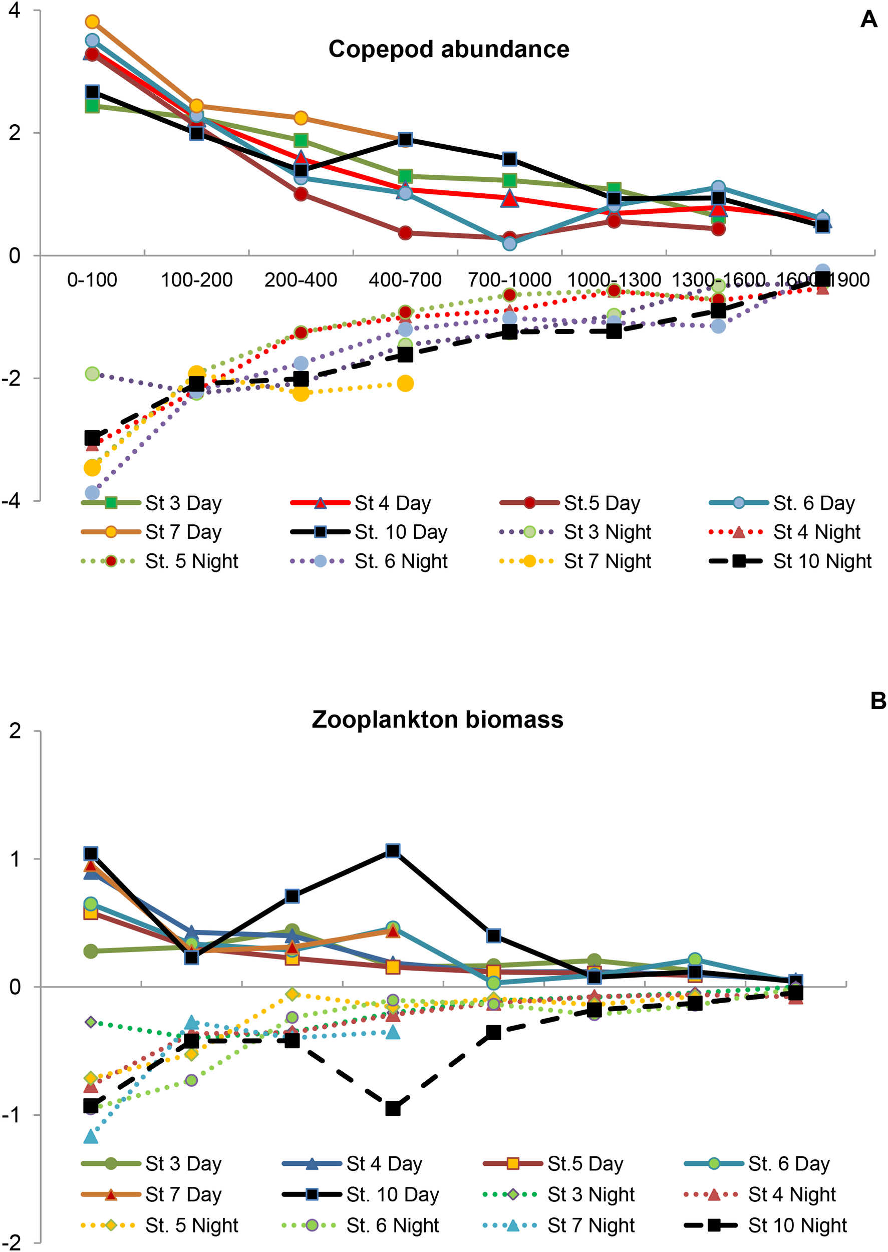
Vertical profiles of (A) abundance of Copepods as ind.m-3 and (B) Zooplankton biomass as mg.m-3 at the different stations analyzed (after Log transformed) from the epipelagic zone to 1900 m depth.
Using the hierarchical clustering of the dominant zooplankton groups at the different layers, we found that the upper 700 m was segregated (55% of similarity) from the layers below (Figure 8). Three main groups were observed: (1) the upper epipelagic (0–100 m depth with 78% of similarity), the 100 to 700 m depth layers (70% of similarity), and below them to 1900 m depth (68%). The NMDS analysis also showed the three groups in which the epipelagic and the mesopelagic layers to 700 m depth were segregated from the other layer (Figure 8). The similarity was also high (72%) from 700 m to 1600 m depth, either by day- and nighttime. Nevertheless, slight differences were observed in the deepest strata (1600-1900m) between day- and nighttime.
Figure 8
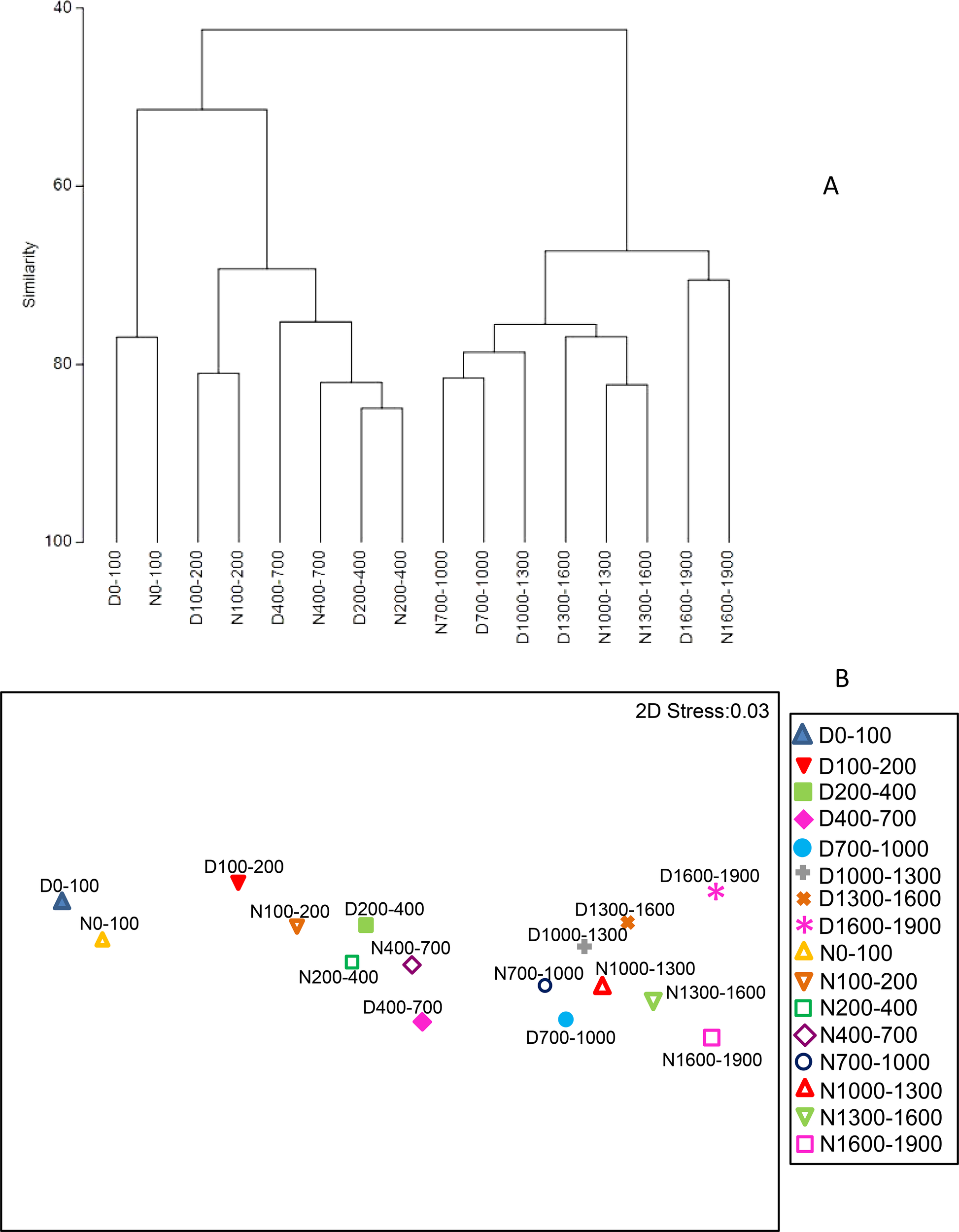
Zooplankton vertical distribution abundance (ind m−3). (A) Hierarchical clustering of the zooplankton community at each sampled layer and (B) non-metric MDS by day- (D) and nighttime (N), after averaging all stations, using fourth root transformation and a resemblance of Bray-Curtis similarity index.
3.3.1 Vertical distribution of copepods
We found 36 copepod families from the epipelagic to the bathypelagic layer (Supplementary Table S2), distributed in 26 calanoids and 10 non-calanoids, and 88 genera, 68 calanoids and 20 non-calanoids. We also identified 255 species of copepods (215 calanoids and 40 non-calanoids), but only 51% of them showed a contribution higher than 1%, and 30% higher than 3%. Sixty species of copepods were not found during the day.
Rank of the copepod species decreased northward (Supplementary Figure S1) while abundance increased. During the day, the highest diversity was found from 100 to 400 m depth (3.2; Table 2), although the highest number of species was found in the layer below (400-700m with 104 species). The lowest diversity was found in the 700–1000 layer during the day (2.4) and in the deepest strata (1600–1900 m depth). During the night the highest diversity was found from 100 to 200 m depth (3.4), close to the value found in the 400–700 m layer (3.1). A high diversity was also observed in the deepest strata (almost 3 at night) although we found quite low abundance of copepods there.
Fifty dominant taxa (>1%) representing more than 85% of the total community abundance were included in a shade plot matrix (Figure 9) combining with their abundances at the different layers during day- and nighttime. First, we observed the highest concentration of the dominant taxa in the upper 100 m layer but also the segregation of the upper 700 m layer from those species distributed below. This pattern was also observed in their vertical distribution during day- and nighttime. The smaller copepods dominated in the upper 100 m layer where different species of Paracalanus, Clausocalanus, Calocalanus and Ctenocalanus were abundant. Some organisms living in the epipelagic strata were moving up and down around the upper 200 m depth such as Centropages typicus or congeneric species of Clausocalanus and Paracalanus. Among the non-calanoids, Corycaeidae spp. predominated also in the epipelagic layer (data not shown). However, Oithona spp. and Oncaea spp. were found deeper (Table 3). The bulk of copepods showed segregation in the upper 700 m layer with some of them dispersed by the whole water column during the day (e.g., Oncaea media, Oithona setigera, or Triconia spp.), increasing their abundances at night in the upper layers. On the other hand, several copepods showed a higher abundance in the upper layers during the night such as Rhincalanus cornutus, some species of Pleuromamma, Metridia, Scolecithricella and Heterorhabdus, which were found in deeper layers during the day (Supplementary Figure S2). Large copepods such as Euchirella spp., Paraeuchaeta spp., or Gaetanus spp. were rather abundant during the day in the 400 to 700 m layer and deeper, and they were also found during the night in the upper 100 m layer. A bimodal distribution was found in some of them such as P. sewelli, Subeucalanus pileatus, Heterorhabdus norvegicus, and C. finmarchicus, or even more chaotic distribution as it was in Metridia curticauda (Supplementary Figure S2). Some copepods showing quite low abundances (<1 ind·m-3) moved up at night as observed in R. cornutus or M. brevicauda. Others living in twilight layers never reached the epipelagic strata such as different species of Conaea, Tortanus, Spinocalanus, and Nullosetigera. They were more abundant below 400 m depth during the day and just moved to the closer layers during the night.
Figure 9
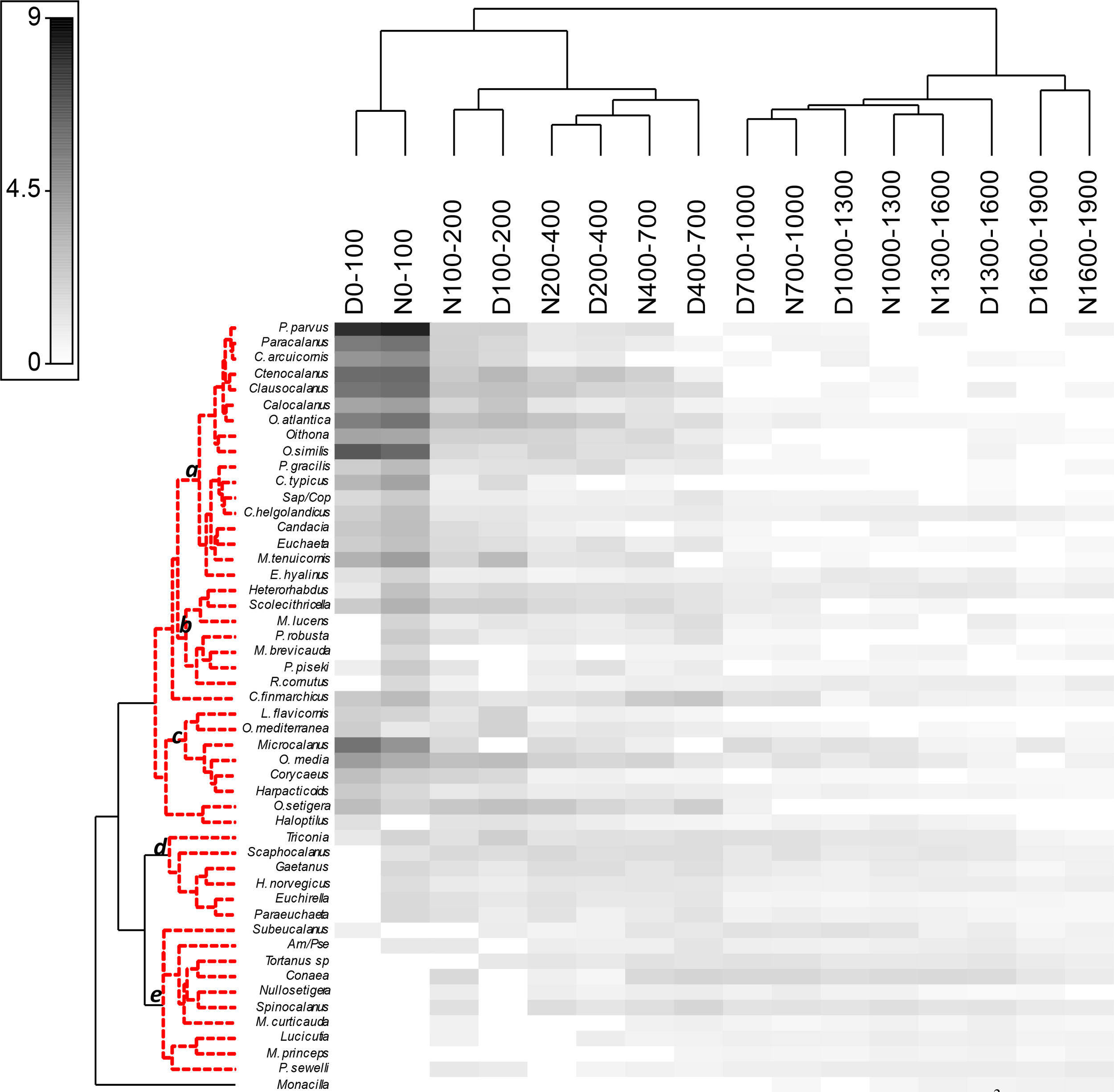
Shade plot of the 50 dominant copepod taxa (>1%; abundance as ind·m-3) related to their strata of preference after fourth root transformed data during day- and nighttime hauls. The hierarchical clustering (simprof test) was obtained using a resemblance matrix and the association index among the dominant taxa. The horizontal axis shows the different strata (m) during day- and nighttime using the Bray Curtis similarity. Amallothrix (Am), Pseudoamallotrhix (Pse), Sapphirina (Sap) and Copilia (Cop) are in abbreviation. Besides the species the genera are indicated as the rest of their own taxa.
Table 3
| Copepod taxa | 0–200 D | 200–400 D | 400–700 D | 700–1000 D | 1000–1600 D | 1600–1900 D | 0–200 N | 200–400 n | 400–70 N | 700–1000 N | 1000–1600 N | 1600–1900 N |
|---|---|---|---|---|---|---|---|---|---|---|---|---|
| C. helgolandicus | 2.05 | 0.08 | 0.16 | 0.03 | 0.17 | 0.12 | 5.41 | 0.09 | 0.13 | 0.03 | 0.14 | 0.02 |
| C. finmarchicus | 2.87 | 0.83 | 6.53 | 0.81 | 0.02 | + | 6.67 | 0.6 | 4.49 | 0.86 | 0.08 | + |
| M. tenuicornis | 17 | 0.43 | + | 0.04 | – | – | 25 | 0.37 | 0.9 | – | – | – |
| Neocalanus | 3.3 | 0.09 | 0.02 | + | + | + | 2.43 | 0.08 | + | + | + | + |
| Calocalanus | 22 | 0.12 | 0.03 | – | – | – | 24 | 0.31 | 0.42 | + | – | – |
| P. denudatus | 70 | 0.08 | + | – | – | – | 78 | 0.12 | 0.04 | + | – | – |
| P. parvus | 317 | 0.42 | + | + | – | – | 369 | 0.18 | 0.71 | + | – | – |
| E. hyalinus | 0.33 | 0.04 | 0.05 | 0.07 | 0.18 | + | 1.25 | + | 0.08 | 0.04 | 0.1 | + |
| P. sewelli | 0.06 | + | 0.02 | 0.06 | 0.11 | 0.13 | 0.09 | – | 0.04 | 0.06 | 0.1 | 0.17 |
| R. cornutus | – | 0.02 | 0.05 | 0.07 | 0.13 | 0.02 | 0.81 | 0.05 | 0.07 | 0.08 | 0.08 | 0.1 |
| Subeucalanus | 0.07 | 0.03 | 0.18 | 0.56 | 0.36 | + | – | 0.02 | 0.34 | 0.47 | 0.27 | 0.03 |
| Microcalanus | 90 | 0.48 | + | 1.41 | 0.36 | 0.41 | 35 | 1.22 | 0.06 | 0.33 | 0.22 | + |
| C. arcuicornis | 33 | 0.13 | + | – | – | – | 44 | 0.04 | – | – | – | – |
| C. pergens | 49 | 1 | 0.52 | – | – | – | 55 | 5.08 | 1.31 | – | – | – |
| C. vanus | 111 | 7.46 | 0.03 | – | – | – | 112 | 4.34 | 3.39 | – | – | – |
| Aetideus | 2.08 | 0.42 | 0.13 | – | – | – | 0.6 | 0.12 | 0.1 | + | – | – |
| Chiridius | – | – | 0.06 | + | – | – | + | 0.07 | 0.09 | 0.04 | – | – |
| Euchirella | 0.1 | 0.19 | 0.32 | + | + | 0.02 | 1.04 | 0.52 | 0.18 | 0.02 | + | – |
| Gaetanus | 0.08 | 0.84 | 0.78 | 0.23 | 0.05 | + | 1.04 | 0.9 | 0.31 | 0.11 | 0.12 | 0.05 |
| Euchaeta | 2.36 | 0.79 | 0.33 | + | + | + | 5.24 | 0.2 | 0.06 | + | + | + |
| Paraeuchaeta | 0.03 | 0.03 | 0.5 | 0.03 | 0.02 | + | 1.02 | 0.5 | 0.14 | 0.09 | 0.05 | + |
| Undeuchaeta | 1.22 | 0.03 | 0.28 | 0.09 | 0.04 | 0.02 | 2.49 | 0.22 | 0.05 | 0.07 | 0.05 | + |
| Amallothrix | – | 0.05 | 0.39 | 0.07 | 0.1 | 0.07 | 0.21 | 0.07 | 0.05 | 0.06 | 0.09 | 0.02 |
| S. brevicornis | – | 0.26 | 0.3 | 0.06 | 0.03 | 0.04 | 0.21 | 0.19 | 0.15 | 0.06 | 0.03 | + |
| Scaphocalanus | 0.47 | 0.8 | 0.83 | 0.2 | 0.22 | 0.08 | 0.88 | 1.64 | 0.91 | 0.79 | 0.32 | 0.03 |
| Scolecithricella | 4.47 | 0.86 | 0.45 | 0.14 | + | + | 12 | 1.43 | 1.39 | 0.09 | + | + |
| Monacilla | – | – | – | – | + | 0.05 | – | – | – | + | 0.03 | 0.05 |
| Spinocalanus | – | 0.31 | 1.91 | 0.51 | 0.48 | 0.25 | 0.34 | 0.9 | 0.76 | 0.57 | 0.66 | 0.15 |
| H. norvergicus | 0.03 | 0.28 | 0.25 | 0.05 | 0.09 | 0.05 | 0.5 | 0.33 | 0.3 | 0.03 | 0.08 | 0.08 |
| Heterorhabdus. | 0.92 | 0.82 | 0.42 | 0.13 | 0.17 | 0.08 | 5.23 | 0.9 | 0.72 | 0.21 | 0.31 | 0.11 |
| L. curta | – | 0.07 | 0.02 | 0.04 | 0.02 | + | 0.02 | + | + | 0.03 | 0.04 | + |
| L. flavicornis | 2.88 | 0.06 | + | – | – | – | 1.32 | + | 0.02 | – | – | – |
| L. wolfendini | – | – | – | 0.02 | 0.03 | + | – | – | 0.01 | + | 0.03 | 0.01 |
| M. lucens | 0.18 | 0.07 | 0.83 | 0.02 | 0.06 | + | 1.25 | 0.13 | 0.34 | 0.05 | 0.02 | + |
| P. abdominalis | 0.13 | 0.13 | 0.2 | 0.02 | + | – | 1.34 | 0.07 | 0.05 | + | + | + |
| P. gracilis | 2.26 | 1.26 | 0.16 | + | + | – | 7 | 0.67 | 0.08 | + | + | – |
| P. piseki | 0.03 | 0.57 | 0.11 | + | + | – | 2.67 | 0.09 | 0.03 | + | + | – |
| Candacia | 3.17 | + | 0.03 | + | – | – | 6 | 0.05 | + | – | 0.02 | – |
| Acartia | 4.48 | + | – | – | – | – | 3.33 | – | – | – | – | – |
| Nullosetigera | – | 0.02 | 0.09 | 0.03 | + | – | 0.04 | 0.07 | 0.07 | 0.1 | 0.02 | + |
| Tortanus | 0.1 | 0.16 | 0.38 | 0.65 | 0.35 | 0.23 | – | 0.31 | 0.57 | 0.6 | 0.27 | 0.07 |
| O. atlantica | 72 | 4.39 | 0.92 | 0.03 | + | – | 94 | 8.19 | 0.5 | 0.09 | + | – |
| O. setigera | 10 | 2 | 3.79 | 0.05 | – | – | 4.35 | 5.93 | 0.94 | – | – | – |
| O. similis | 159 | 0.73 | 0.39 | – | + | – | 115 | 2.43 | 0.77 | – | – | – |
| O. tenuis | 19 | 0.69 | 0.08 | + | + | + | 12 | 2.22 | 1.35 | – | – | – |
| O. media | 31 | 1.68 | 0.37 | 0.14 | 0.09 | – | 18 | 2.79 | 2.59 | 0.64 | 0.32 | 0.05 |
| Triconia | 1.86 | 0.64 | 0.98 | 0.84 | 0.32 | 0.02 | 1.36 | 0.44 | 0.61 | 0.77 | 0.34 | + |
| Conaea | – | + | 2.26 | 2.12 | 1.25 | 0.52 | 0.65 | 0.05 | 1.37 | 2.05 | 1.61 | 0.13 |
Abundance of the dominant copepod taxa (ind m-3) at each analyzed layer during day and nighttime (≤0.01).
According to the clusters of Figure 9, the vertical distribution of copepods indicated five dominant copepod assemblages (Figure 10). We found a large group relevant in the upper layer displaying three main different assemblages: (1) Group a (34%) occupied the epipelagic layer having high and similar abundances during day-and nighttime. It was the dominant group with 17 taxa (69% of similarity). This group was represented by different species of Paracalanus, Clausocalanus, Calocalanus, Ctenocalanus, and Candacia. At this layer, we also found Euchaeta, several Oithona. as well as C. helgolandicus, C. typicus and M. tenuicornis. (2) Group b (14%) inhabited deeper layers during day but being quite abundant at night in the upper layers. It was formed by seven taxa (60% of similarity) which were moving upward during the night into the upper 100 m layer. They were relevant migrants represented by different species of Metridia and Pleuromamma, as well as Scolecithricella and Rhincalanus. Separated to this group, C. finmarchicus was found in the northern station showing a bimodal distribution during day-and nighttime, also indicating a migratory behavior (Figure 10). The higher concentration of this species was found in the 400–700 m layer during the day but also in the upper 100 m layer where part of their deep population moved at night. (3) Group c (16%) was more abundant at the surface during the day dispersing at night. It was composed by eight taxa (50% of similarity) predominating in the epipelagic zone during the day but dispersed in the upper 700 m depth during the night. The best represented taxa of this group were from Oncaea, Microcalanus, Haloptilus, and Corycaeidae spp. (4) Group d (12% of the dominant taxa) was formed by large vertical migrants showing bimodal distribution, moving to the upper layers at night and living in meso- and bathypelagic zones during the day. It was composed by six taxa with a 50% of similarity (Euchirella, Paraeuchaeta, Scaphocalanus. and Gaetanus). (5) Group e was observed in the twilight layer (20%) but with slight vertical movements. It was formed by 10 taxa and 62% of similarity. They never reached the epipelagic layer, always living in the mesopelagic layer. It was dominated by different species of Tortanus, Spinocalanus, Nullosetigera and Conaea, among others. Multiple plots of the different diel vertical distribution of all copepod assemblages are detailed in the Supplementary Material (Supplementary Figure S2). Finally, although showing quite low abundances, other copepods such as those of the genus Monacilla spp. inhabited in the bathypelagic layer at any time (below 1000 m depth) with slight increasing during the night (Figure 10).
Figure 10
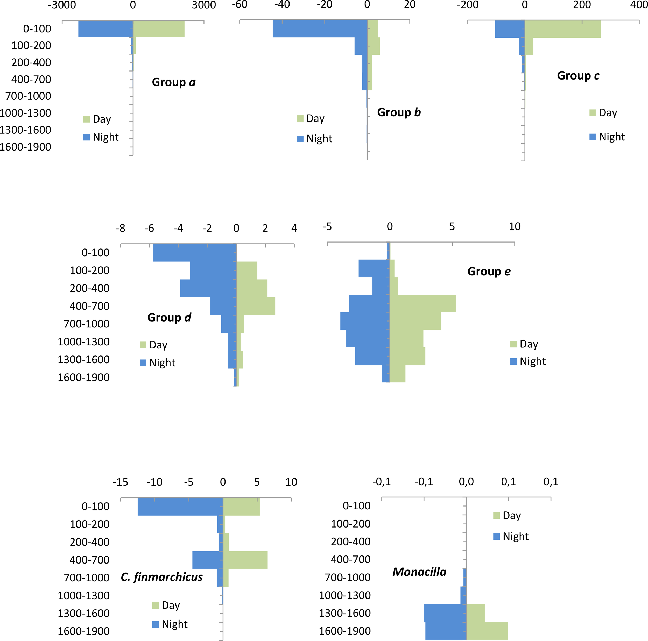
Copepod vertical distribution assemblages (ind m-3) observed at each stratum during day- and nighttime obtained using the previous shade plot of Figure 9.
Simper analysis showed the contribution to the dissimilarity of the representative taxa among day and night indicating the dominant copepods at the epipelagic, mesopelagic, and bathypelagic layers (Table 4). Accordingly, P. parvus, Calocalanus spp, Clausocalanus spp., M. tenuicornis, Ctenocalanus spp., and Oithona spp. dominated the upper 200 m layer. In the mesopelagic zone, C. finmarchicus dominated the mid-depth during day- and nighttime. They were only observed in high abundances in the northern St. 10 jointly with Metridia lucens , Heterorhabdus norvegicus, and Spinocalanus longicornis. Below 1000 m depth, different species of Conaea, Microcalanus, and Spinocalanus were dominant. Further south, Oncaea spp. were present in the whole water column, Pleuromamma spp., Euchirella spp., and Scaphocalanus spp. dominated the mesopelagic layer as well as P. sewelli, S. pileatus, Spinocalanus spp., and Tortanus spp. in the deepest layers. The contribution to similarity of the most representative copepod taxa is also indicated for the different studied layers (Supplementary Table S3) showing their depth preferences during day- and nighttime.
Table 4
| Groups ep day & night (0-200m) | Average dissimilarity (AD) = 62% | ||||
|---|---|---|---|---|---|
| Ep day | Ep night | ||||
| Copepod taxa | Av. Abund | Av. Abund | Av. Diss | Diss/SD | Contrib% |
| Oithona | 11.5 | 11.5 | 7.1 | 1.1 | 11.4 |
| P. parvus | 10.5 | 10.0 | 6.8 | 1.0 | 11.0 |
| Ctenocalanus | 6.3 | 6.2 | 4.1 | 1.2 | 6.7 |
| P. denudatus | 4.2 | 4.2 | 3.4 | 0.8 | 5.6 |
| C. pergens | 3.8 | 3.6 | 2.8 | 0.9 | 4.5 |
| C. arcuicornis | 3.2 | 4.0 | 2.8 | 1.0 | 4.5 |
| Oncaea | 3.6 | 3.9 | 2.4 | 1.2 | 3.9 |
| Calocalanus | 3.7 | 3.2 | 2.2 | 1.6 | 3.5 |
| Microcalanus | 2.8 | 2.7 | 2.1 | 0.6 | 3.5 |
| M. tenuicornis | 3.3 | 3.3 | 2.1 | 1.2 | 3.4 |
| Pleuromamma | 2.6 | 4.4 | 2.0 | 1.3 | 3.3 |
| Groups UMs day& night (200–400 m) | AD =55% | ||||
|---|---|---|---|---|---|
| UMs Day | UMs Night | ||||
| Copepod taxa | Av. Abund | Av. Abund | Av. Diss | Diss/SD | Contrib% |
| Oithona | 2.3 | 4.0 | 8.2 | 1.1 | 15.0 |
| C. pergens | 0.6 | 1.5 | 3.6 | 1.2 | 6.5 |
| Ctenocalanus | 1.4 | 1.2 | 3.3 | 1.0 | 6.1 |
| Pleuromamma | 2.2 | 2.1 | 3.0 | 1.6 | 5.5 |
| Oncaea | 1.3 | 1.9 | 2.6 | 1.3 | 4.7 |
| Metridia | 0.8 | 0.5 | 2.4 | 0.8 | 4.3 |
| Scaphocalanus | 0.7 | 0.9 | 1.8 | 1.6 | 3.3 |
| C. finmarchicus | 0.4 | 0.4 | 1.8 | 0.6 | 3.3 |
| Spinocalanus | 0.4 | 0.7 | 1.6 | 1.3 | 2.9 |
| Heterorhabdus | 0.7 | 0.8 | 1.5 | 1.8 | 2.7 |
| Scolecithricella | 0.8 | 1.0 | 1.4 | 1.7 | 2.6 |
| Microcalanus | 0.3 | 0.6 | 1.4 | 0.9 | 2.5 |
| Groups CMs day & night (400–700 m) | AD =56% | ||||
|---|---|---|---|---|---|
| CMs Day | CMs Night | ||||
| Copepod taxa | Av. Abund | Av. Abund | Av. Diss | Diss/SD | Contrib% |
| C. finmarchicus | 1.2 | 0.9 | 4.9 | 0.6 | 8.8 |
| Oithona | 1.5 | 1.4 | 4.6 | 1.1 | 8.2 |
| Conaea | 1.2 | 1.0 | 3.1 | 1.2 | 5.5 |
| Spinocalanus | 0.9 | 0.8 | 2.8 | 1.6 | 5.0 |
| Metridia | 1.1 | 1.1 | 2.7 | 1.2 | 4.9 |
| Oncaea | 1.1 | 1.6 | 2.6 | 1.0 | 4.7 |
| Pleuromamma | 1.3 | 1.1 | 2.3 | 1.7 | 4.0 |
| C. pergens | 0.3 | 0.7 | 2.0 | 1.0 | 3.6 |
| Tortanus | 0.4 | 0.5 | 1.8 | 1.0 | 3.2 |
| Scolecithricella | 0.6 | 0.8 | 1.6 | 1.1 | 2.9 |
| Scaphocalanus | 0.8 | 0.9 | 1.6 | 1.3 | 2.8 |
| Ctenocalanus | 0.1 | 0.8 | 1.5 | 0.5 | 2.8 |
| Heterorhabdus | 0.5 | 0.7 | 1.5 | 1.2 | 2.7 |
| Groups LMs day& night (700–1000 m) | AD =54% | ||||
|---|---|---|---|---|---|
| LMs Day | LMs Night | ||||
| Copepod taxa | Av. Abund | Av. Abund | Av. Diss | Diss/SD | Contrib% |
| Conaea | 1.1 | 1.3 | 5.0 | 1.5 | 9.2 |
| Oncaea | 0.9 | 0.8 | 4.1 | 1.4 | 7.6 |
| Metridia | 0.6 | 1.1 | 3.6 | 1.2 | 6.6 |
| Scaphocalanus | 0.4 | 0.9 | 3.1 | 1.6 | 5.8 |
| C. finmarchicus | 0.4 | 0.5 | 3.1 | 0.7 | 5.7 |
| Tortanus | 0.5 | 0.5 | 3.0 | 1.0 | 5.6 |
| Microcalanus | 0.5 | 0.3 | 3.0 | 0.8 | 5.5 |
| Spinocalanus | 0.6 | 0.7 | 2.6 | 1.2 | 4.9 |
| Subeucalanus | 0.4 | 0.4 | 2.6 | 0.9 | 4.9 |
| Gaetanus | 0.3 | 0.3 | 1.5 | 1.4 | 2.8 |
| Groups BT day & night (1000–1900 m) | AD =51% | ||||
|---|---|---|---|---|---|
| BTDay | BTNight | ||||
| Copepod taxa | Av. Abund | Av. Abund | Av. Diss | Diss/SD | Contrib% |
| Metridia | 0.6 | 0.7 | 4.4 | 1.1 | 8.7 |
| Conaea | 0.9 | 0.9 | 4.4 | 1.4 | 8.7 |
| Tortanus | 0.4 | 0.4 | 2.8 | 1.4 | 5.5 |
| Oncaea | 0.4 | 0.5 | 2.8 | 1.3 | 5.4 |
| Spinocalanus | 0.6 | 0.6 | 2.7 | 1.3 | 5.4 |
| Microcalanus | 0.3 | 0.2 | 2.6 | 0.6 | 5.1 |
| Subeucalanus | 0.3 | 0.2 | 2.5 | 0.9 | 4.9 |
| P. sewelli | 0.2 | 0.2 | 2.2 | 0.9 | 4.2 |
| Heterorhabdus | 0.3 | 0.4 | 2.1 | 1.4 | 4.2 |
| E. hyalinus | 0.2 | 0.2 | 2.0 | 0.9 | 3.6 |
| Rhincalanus | 0.2 | 0.2 | 1.9 | 1.0 | 3.6 |
Contribution to dissimilarity of the most representative Copepod taxa (cut off 60%) among pairs of samples at each layer by “Day and Night” factor (Ep, Epipelagic; UMs, Upper Mesopelagic; CMs, Central Mesopelagic; LMs, Lower Mesopelagic; BT, Bathypelagic; Av. Abund, Average Abundance).
4 Discussion
A boundary region was found at around 45-47°N in the epipelagic layer as observed from the chlorophyll a, micro-, and mesozooplankton distribution coinciding with the frontal system described by Gaard et al. (2008) and Søiland et al. (2008). As expected, we also notice the bulk of mesozooplankton concentrated in the upper 100 m layer, particularly copepods (Weikert and Koppelmann, 1993). These organisms decreased sharply below the euphotic zone in agreement with earlier data in the North Atlantic Ocean (Weikert and Trinkaus, 1990; Gaard et al., 2008; Bode et al., 2018). Besides, a northward increase of zooplankton abundance and biomass in the epipelagic zone was observed by Clark et al. (2001); Søiland et al. (2008), and Vecchione et al. (2010). We also found a high abundance of copepod nauplii coinciding with the intense phytoplankton bloom in the frontal system; also in agreement with the presence of small stages of copepods found in other frontal areas (see Mackas et al., 1991; Kiørboe, 1993; Sournia, 1994). The predominance of carnivorous zooplankton in the southern region and herbivorous northward was also indicated by Gaard et al., 2008. These differences in zooplankton composition between both regions are also consistent with the associated productivity of temperate oceans (Sumich, 1984; Boudreau et al., 1991) and the increase of zooplankton during spring (Sameoto, 1984; Richardson, 1985; Gislason et al., 2008). However, although large-scale latitudinal and DVM were studied for the zooplankton abundance and biomass (Longhurst and Williams, 1979; Gislason, 2003; Vinogradov, 2005), depth stratified studies of the copepod community were not reported for this area.
4.1 Latitudinal distribution of copepods
We observed differences in the composition of copepods between the southern and northern latitudes (see groups in Figure 5A) and according to Sundby (2000) it could be related to temperature and stratification as two of the most important factors determining the structure of the copepod community. However, although in the epipelagic layer (0–200 m) the copepod community showed different structure among regions, most copepods were, as in our study, cosmopolitan (Bucklin et al., 2010). Among the Calanoids, Clausocalanus spp., and Paracalanus spp. were rather abundant, being P. parvus and their juveniles the dominant copepods in the frontal zone. Among the non-calanoids, Oithona spp. was by far the most abundant copepod, an ubiquitous organism in the world ocean whose information about its distribution pattern is still limited (Gallienne and Robins, 2001). In our study, O. setigera was found in the whole transect while O. tenuis and O. plumifera were found in the southern area. Other species such as O. similis and O. atlantica were only found in the northern area with a southern limit at 47°N.
Some copepods such as C. styliremis or M. tenuicornis were found in the whole area, while C. arcuicornis, N. minor, M. clausi as well as Sapphirina spp., F. rostrata and other Corycaeidae spp. were abundant in the southern stations. They are characteristic species of warm latitudes (Vives and Shmeleva, 2007, 2011; Schnack-Schiel et al., 2010; Wootton and Castellani, 2016). By contrast, in the northern region the latter copepods were absent observing a high abundance of Metridia spp. and C. finmarchicus in agreement with authors working in the area (Gaard et al., 2008; Gislason et al., 2008). C. finmarchicus dominated the northern latitudes replacing C. helgolandicus observed toward the south as expected (Fleminger and Hulsemann, 1977; Conover, 1988; Planque et al., 1997; Beaugrand et al., 2001).
A high abundance of P. parvus was also noticed in other areas of the North Atlantic Ocean also showing a surface distribution (Frost and Fleminger, 1968; Vinogradov et al., 1970; Deevey and Brooks, 1977) which could be related to the warm waters found at the east of the MAR (Pollard et al., 2004). The northeastward trajectory of the North Atlantic currents enables species of southern warmer areas to appear east of the MAR and north the frontal system. As a result, the northern limit of warm water species could be observed further north in the eastern side than the western side of the ridge. Accordingly, the copepod distribution pattern showed a non-symmetrical horizontal distribution, underlining the complexity of the biogeographic area (Beaugrand et al., 2001; Gallienne et al., 2001; Hays et al., 2001; Stemmann et al., 2008; Barnard et al., 2011). In any case, Paracalanus spp. are a widespread cosmopolitan epipelagic species, living in high chlorophyll conditions (Siokou-Frangou et al., 2010), which could be found forming intense patches and being well adapted to many ecosystems and food resources (Siokou et al., 2019).
4.2 Copepod diversity
To our knowledge, the number of genera found in the present study was slightly higher than previous studies carried out in the North Atlantic (Gaard et al., 2008). This might be probably due to our extensive sampled area from low latitudes (20°N) and to the important depth range of our study (Roe, 1984; Woodd-Walker et al., 2002). In similar latitudes, Grice and Hulsemann (1965) found 66 calanoid genera between 0 and 5000 m depth, most of them in the upper 2000 m depth, close to our record of 68 calanoid genera.
In relation to the rather large area covered from subtropical to temperate latitudes, we found only one third of the copepod species and one half of the genera in the northern stations. Copepod diversity as the number of copepod genera and species declined northward as previously observed in different Atlantic areas (Angel, 1993; Pierrot-Bults, 1997; Woodd-Walker et al., 2002; Bode et al., 2018). Variable diversity and less clear latitudinal trend were observed north of 40°N (Woodd-Walker et al., 2002). This could be explained by the complex distribution of currents, the warmer water supplied from southern areas (Pollard et al., 2004), and the intensity of the frontal system (Beaugrand and Ibañez, 2002). The west-east asymmetry also confirmed the different diversity of calanoids on either side of the MAR forming different species association (Beaugrand et al., 2001, 2002).
The highest diversity observed from 100 to 700 m depth during daytime and at the 100–200 m layer at night is also in agreement with other authors working in the subtropical and temperate oceans (Gaard et al., 2008; Bode et al., 2018). The concentration of available food but also environmental gradients decreasing with depth, could be behind the decline of the number of ecological niches and consequently in species diversity (Longhurst, 1985). It was interesting to observe a high diversity in the deepest layers during the night (3, Table 2) which can be due to the low abundance and the inhabiting species of copepods probably reaching up from below depths.
4.3 Vertical distribution of copepods
We found a large number of copepods living in the upper 100 m layer. Group a was formed by species quite abundant during the day in the epipelagic layer (35%). This abundant group was mainly composed by different species of Paracalanus, Clausocalanus, Ctenocalanus and Calocalanus. Another group seemed to display a reverse migration since they were rather abundant during the day in the epipelagic layer and at night were dispersed by the different adjacent layers in quite low abundances. This was the case of Group c composed by different species of Oithona, Oncaea and Microcalanus. Because of this, it was not easy to define their vertical movements. By opposite, some species were rather abundant in the epipelagic layer particularly during the night but in low abundance during the day (Group b). Most copepods living in the upper layers were associated with the highest food abundance as it was the case of Paracalanus spp. and Clausocalanus spp. (omnivores-herbivores) and Oithona spp. and Oncaea spp. (detritivores), reflecting their trophic regime disparity (Kiørboe, 2011; Benedetti et al., 2016). Fernández de Puelles et al. (2023) found, in lower latitudes, many of these copepods moving daily around the upper 100 m depth, and increasing their abundances during the night in the upper 50 m. However, we were not able to observe this migration due to our wider sampling strategy in this layer.
We also found strong interzonal migrants which were a group of species moving from meso- or bathypelagic layers toward the epipelagic layer at night (Group d, 13%). We also showed that each stratum was inhabited by different copepod assemblages, indicating differences among day- and nighttime. We found two groups of strong migrants moving from deep layers to the surface, one with bimodal vertical profiles (Group d: different species of Euchirella, Gaetanus, Paraeuchaeta, Scaphocalanus and H. norvegicus) and the other with also vertical migration during the night (Group b: R. cornutus, M. lucens, M. brevicauda and P. robusta or P. piseki). All of these were migratory copepods too, which were found in high abundances in the epipelagic waters at night (15%), exhibiting similar vertical migrations as in tropical and subtropical latitudes (Deevey and Brooks, 1977; Roe, 1984; Roe et al., 1984; Longhurst et al., 1990; Fernández de Puelles et al., 2023).
We also observed the group of species characteristic in the twilight layers (Group e: 21%) showing closer abundances during day- and nighttime (such as species of Conaea, Tortanus, Nullosetigera, Subeucalanus, P. sewelli or M. princeps). They could be present slightly shallower at night but never reaching the upper 100 m layer, exhibiting a similar vertical distribution to the ones found at lower latitudes (Roe, 1984; Roe et al., 1984; Fernández de Puelles et al., 2023).
Although in low abundances, other copepods were always living in bathypelagic layers such as Monacilla. Some deep copepods such as P. sewelli in our data exhibited different vertical distribution than in lower latitudes (Fernández de Puelles et al., 2023). In this sense, it is important to mention that some deep copepods such as Euchirella spp., Heterorhabdus spp., or Gaetanus spp. showed differences in their vertical distribution with latitude, usually becoming deeper in southern regions (Gride, 1963; Bucklin et al., 2010). We also found that deep copepods collected in southern stations did not appear in the northern ones (e.g., T. mayumbaensis, P. sewelli, different species of Scottocalanus or Nullosetigera), in agreement with earlier studies in close areas (Gaard et al., 2008). A similar pattern was observed for decapods and ostracods in different regions of the North Atlantic Ocean (Foxton, 1972; Fasham and Angel, 1975).
Particular mention is given to the well-studied C. finmarchicus (Marshall and Orr, 1972) which was highly abundant in northern latitudes (Gaard et al., 2008). In our study, C. finmarchicus showed a bimodal vertical profile, more abundant at night in the upper layer (Figure 10). This copepod is known to display a large variability in the vertical distribution of their developmental stages, including diel variation (Kaartvedt, 1996; Mauchline, 1998). The apparent absence of regular DVM of some species (e. g. C. helgolandicus in our data), does not necessarily mean that a population does not migrate vertically since they could change their vertical displacements with latitude (Roe et al., 1984). There are many difficulties in interpreting vertical distribution patterns since it is possible that apparent non-migrants move acyclically or migrate every two days. The vertical distribution patterns of copepods could vary in time and space exhibiting a complex behavior and sometimes showing irregular and chaotic movements (Sameoto, 1976; Roe and Badcock, 1984).
In summary, this study provides the vertical distribution of the dominant copepods in the North Atlantic Ocean across an extensive region and spanning down to bathypelagic layers. We found that almost half of the total copepods were living in the epipelagic layer while others were abundant in deeper layers during the day moving or not during the night towards the surface. This pattern was close to the distribution observed in tropical and subtropical latitudes at the basin scale (Fernández de Puelles et al., 2023). In this study, we observed a latitudinal decreasing gradient northward in the number of genera and species, and an increasing gradient in their abundances. Small copepod nauplii and Paracalanus parvus predominated in the frontal zone found between 45 and 47°N, while in the northern region, Calanus finmarchicus and several Oithona dominated. South of this latitude, warmer species such as C. helgolandicus, N. minor, and M. clausi were more abundant. Deep copepods were also of importance in the vertical distribution and structure of the community with the larger species living in meso- and bathy-pelagic layers, moving upward at night. Accordingly, we found at least five groups in their vertical distribution: (1) the non-migrant epipelagic copepods, (2) those migrant copepods observed in high abundances in the epipelagic layer only at night and in deeper layers during the day, (3) the copepods abundant in the epipelagic layer by day performing reverse migrations, (4) the strong migrants moving from the meso- and bathypelagic layers to the epipelagic zone at night and finally (5) those just moving into the twilight zone. Here, we disentangled the structure of these communities in the above related five groups shedding light about their role in the ocean as epipelagic non-migrant consumers and those performing strong diel vertical migrations, being also key copepods promoting active flux (Turner, 2015). Accordingly, all of them are essential contributors to the ocean biogeochemistry and carbon flux through the water column. Finally, we underline the need for taxonomic studies in more extensive areas and seasons for further understanding of the role of these organisms in the biological carbon pump.
Statements
Data availability statement
The raw data supporting the conclusions of this article will be made available by the authors, without undue reservation.
Ethics statement
The manuscript presents research on animals that do not require ethical approval for their study.
Author contributions
MLFP: Conceptualization, Funding acquisition, Validation, Software, Investigation, Resources, Writing – review & editing, Project administration, Writing – original draft, Supervision, Data curation, Visualization, Formal Analysis, Methodology. MG: Formal Analysis, Methodology, Investigation, Writing – original draft. MC-R: Supervision, Software, Writing – review & editing, Validation. SH-L: Formal Analysis, Validation, Supervision, Writing – review & editing, Funding acquisition, Conceptualization.
Funding
The author(s) declare financial support was received for the research, and/or publication of this article. This work was supported by the projects “Biomass and Active flux study in the Bathypelagic zone of the North Atlantic Ocean” (BATHYPELAGIC, CTM 2016-78853-R) and “Disentangling Seasonality and Active Flux In the Ocean (DESAFÍO, PID2020-118118RB-100) from the Spain Ministry of Science and Innovation, and by the European Union (Horizon 2020 Research and Innovation Programme) through projects SUMMER (Grant Agreement 817806) and TRIATLAS (Grant Agreement 817578).
Acknowledgments
We would like to acknowledge the crew and staff on board of the R/V Sarmiento de Gamboa, particularly to the “Unidad deTecnologı́a Marina (UTM)” for their valuable support during the survey. We also wish M. Mar Santandreu, technical staff of the“Centro Oceanográfico de Baleares (COB), for her help on board and in the sampling analysis of microzooplankton and its biomass. Also to Dra. Itziar Alvarez from the COB who helped us with some figures. We also wish to acknowledge Prof. E. Guerra for his suggestions and support with the statistical treatment and multivariate analysis with the Primer 7, and to the Working Group of Zooplankton ecology (WGZE) of the International Council for the Exploration of the Sea (ICES) for their constant support.
Conflict of interest
The authors declare that the research was conducted in the absence of any commercial or financial relationships that could be construed as a potential conflict of interest.
Generative AI statement
The author(s) declare that no Generative AI was used in the creation of this manuscript.
Any alternative text (alt text) provided alongside figures in this article has been generated by Frontiers with the support of artificial intelligence and reasonable efforts have been made to ensure accuracy, including review by the authors wherever possible. If you identify any issues, please contact us.
Publisher’s note
All claims expressed in this article are solely those of the authors and do not necessarily represent those of their affiliated organizations, or those of the publisher, the editors and the reviewers. Any product that may be evaluated in this article, or claim that may be made by its manufacturer, is not guaranteed or endorsed by the publisher.
Supplementary material
The Supplementary Material for this article can be found online at: https://www.frontiersin.org/articles/10.3389/fmars.2025.1641055/full#supplementary-material
References
1
Anderson M. J. Gorley R. N. Clarke K. R. (2008). PERMANOVA+ for PRIMER: Guide to Software and Statistical Methods (Plymouth: PRIMER-E).
2
Angel M. V. (1993). Biodiversity of the pelagic ocean. Conserv. Biol.7, 760–772. Available online at: http://www.jstor.org/stable/2386808.
3
Barnard R. Batten S. Beaugrand G. Buckland C. Conway D. Edwards M. et al . (2011). Continuous plankton records: Plankton atlas of the North Atlantic Ocean, (1958-1999). II. Biogeographical charts. Mar. Ecol. Prog. Ser. MEPS Suppl. 11–75
4
Beaugrand G. Ibañez F. (2002). Spatial dependence of calanoid copepod diversity in the North Atlantic Ocean. Mar. Ecol. Prog. Ser.232, 197–211. Available online at: https://www.int-res.com/abstracts/meps/v232/p197-211/.
5
Beaugrand G. Ibañez F. Lindley J. A. (2001). Geographical distribution and seasonal and diel changes in the diversity of calanoid copepods in the North Atlantic and North Sea. Mar. Ecol. Prog. Ser.219, 189–203. Available online at: https://www.int-res.com/abstracts/meps/v219/p189-203/.
6
Beaugrand G. Ibañez F. Lindley J. A. Reid P. C. (2002). Diversity of calanoid copepods in the North Atlantic and adjacent seas: species associations and biogeography. Mar. Ecol. Prog. Ser.232, 179–195. Available online at: https://www.int-res.com/abstracts/meps/v232/p179-195/.
7
Beaugrand G. Reid P. C. Ibañez F. Planque B. (2000). Biodiversity of North Atlantic and North Sea calanoid copepods. Mar. Ecol. Prog. Ser.204, 299–303. Available online at: https://www.int-res.com/abstracts/meps/v204/p299-303/.
8
Benedetti F. Gasparini S. Ayata S. D. (2016). Identifying copepod functional groups from species functional traits. J. Plankton Res.38, 159–166. doi: 10.1093/plankt/fbv096
9
Bode M. Hagen W. Cornils A. Kaiser P. Auel H. (2018). Copepod distribution and biodiversity patterns from the surface to the deep sea along a latitudinal transect in the eastern Atlantic Ocean (24°N to 21°S). Prog. Oceanogr.161, 66–77. doi: 10.1016/j.pocean.2018.01.010
10
Boltovskoy D. (1981). Atlas del zooplankton del Atlántico Sudoccidental y métodos de trabajo con el zooplancton marino. Ed. BoltovskoyD. (Mar de la Plata, Argentina: INIDEP Publisher), 933.
11
Boudreau P. R. Dickie L. M. Kerr S. R. (1991). Body-size spectra of production and biomass as system-level indicators of ecological dynamics. J. Theor. Biol.152, 329–339. doi: 10.1016/S0022-5193(05)80198-5
12
Bucklin A. Nishida S. Schnack-Schiel S. Wiebe P. H. Lindsay D. Machida R. J. et al . (2010). “ A Census of Zooplankton of the Global Ocean,” in Life in the World’s Oceans. Ed. McIntyreA. D. (Oxford, United Kingdom: Blackwell Publisher), 247–263. doi: 10.1002/9781444325508.ch13
13
Clark D. R. Aazem K. V. Hays G. C. (2001). Zooplankton Abundance and Community Structure Over a 4000 km transect in the North-east Atlantic. J. Plankton Res.23, 365–372. doi: 10.1093/plankt/23.4.365
14
Clarke K. R. Gorley R. N. (2006). PRIMER v6: User Manual/Tutorial (Plymouth: PRIMER-E).
15
Clarke K. R. Somerfield P. J. Gorley R. N. (2008). Testing of null hypotheses in exploratory community analyses: similarity profiles and biota-environment linkage. J. Exp. Mar. Biol. Ecol.366, 56–69. doi: 10.1016/j.jembe.2008.07.009
16
Conover R. J. (1988). Comparative life histories in the genera Calanus and Neocalanus in high latitudes of the northern hemisphere. Hydrobiologia167, 127–142. doi: 10.1007/BF00026299
17
Conway D. (2012). Marine Zooplankton of Southern Britain - Part 2: Arachnida, Pycnogonida, Cladocera, Facetotecta, Cirripeda and Copepoda (Plymouth (UK). Available online at: https://plymsea.ac.uk/id/eprint/5633.
18
Cushing D. H. (1951). The vertical migration of planktonic crustacea. Biol. Rev.26, 158–192. doi: 10.1111/j.1469-185X.1951.tb00645.x
19
Deevey G. B. Brooks A. L. (1977). Copepods of the Sargasso Sea off Bermuda: Species Composition, and Vertical and Seasonal Distribution between the Surface and 2000m. Bull. Mar. Sci.27, 256–291. Available online at: https://www.ingentaconnect.com/content/umrsmas/bullmar/1977/00000027/00000002/art00006.
20
Fasham M. J. R. Angel M. V. (1975). The relationship of the zoogeographic distributions of the planktonic ostracods in the North-east Atlantic to the water masses. J. Mar. Biol. Assoc. Unite. KDm.55, 739–757. doi: 10.1017/S0025315400017380
21
Fernández de Puelles M. L. Gazá M. Cabanellas-Reboredo M. Santandreu M. D. Irigoien X. González-Gordillo J. I. et al . (2019). Zooplankton abundance and diversity in the tropical and subtropical ocean. Diversity (Bs)11, 1–22. doi: 10.3390/d11110203
22
Fernández de Puelles M. L. Gazá M. Santandreu M. Hernández-León S. (2023). Diel vertical migration of copepods in the tropical and subtropical Atlantic Ocean. Prog. Oceanogr.219, 103147. doi: 10.1016/j.pocean.2023.103147
23
Fernández de Puelles M. L. Valdés L. Varela M. Alvarez-Ossorio M. T. Holliday N. (1996). Diel variations in the vertical distribution of copepods off the north coast of Spain. ICES J. Mar. Sci.53, 97–106. doi: 10.1006/jmsc.1996.0009
24
Fleminger A. Hulsemann K. (1977). Geographical range and taxonomic divergence in North Atlantic Calanus (C. helgolandicus, C. finmarchicus and C. glacialis). Mar. Biol.40, 233–248. doi: 10.1007/BF00390879
25
Foxton P. (1972). Observations on the Vertical Distribution of the Genus Acanthephyra (Crustacea: Decapoda) in the eastern North Atlantic, with particular reference to Species of the ‘purpurea’ Group. Proc. R Soc. Edin. Biol.73, 301–313. doi: 10.1017/S0080455X00002356
26
Frost B. W. Fleminger A. (1968). A revision of the genus Clausocalanus: (Copepoda: Calanoida) with remarks on distributional patterns in diagnostic characters. Available online at: https://api.semanticscholar.org/Corpus%20ID:127996548.
27
Gaard E. Gislason A. Falkenhaug T. Søiland H. Musaeva E. Vereshchaka A. et al . (2008). Horizontal and vertical copepod distribution and abundance on the Mid-Atlantic Ridge in June 2004. Deep Sea Res. Part II: Topical Stud. Oceanogr.55, 59–71. doi: 10.1016/j.dsr2.2007.09.012
28
Gallienne C. P. Robins D. B. (2001). Is Oithona the most important copepod in the world’s oceans? J. Plankton Res.23, 1421–1432. doi: 10.1093/plankt/23.12.1421
29
Gallienne C. P. Robins D. B. Woodd-Walker R. S. (2001). Abundance, distribution and size structure of zooplankton along a 20° west meridional transect of the northeast Atlantic Ocean in July. Deep Sea Res. Part II: Topical Stud. Oceanogr.48, 925–949. doi: 10.1016/S0967-0645(00)00114-4
30
Gibb S. W. Cummings D. G. Irigoyen X. Barlow R. G. Fauzi R. Mantoura C. (2001). Phytoplankton pigment chemotaxonomy of the northeastern Atlantic. Deep Sea Res. Part II: Topical Stud. Oceanogr.48, 795–823. doi: 10.1016/S0967-0645(00)00098-9
31
Gislason A. (2003). Life-cycle strategies and seasonal migrations of oceanic copepods in the Irminger Sea. Hydrobiologia503, 195–209. doi: 10.1023/B:HYDR.0000008498.87941.7d
32
Gislason A. Gaard E. Debes H. Falkenhaug T. (2008). Abundance, feeding and reproduction of Calanus finmarchicus in the Irminger Sea and on the northern Mid-Atlantic Ridge in June. Deep Sea Res. Part II: Topical Stud. Oceanogr.55, 72–82. doi: 10.1016/j.dsr2.2007.09.008
33
Grice G. D. Hulsemann K. (1965). Abundance, vertical distribution and taxonomy of calanoid copepods at selected stations in the northeast Atlantic. Proc. Zool. Soc. London146, 213–262. doi: 10.1111/j.1469-7998.1965tb05210.x
34
Gride G. D. (1963). Deep water copepods from the western North Atlantic with notes on five species. Bull. Mar. Sci. Gulf Carib.13, 493–501.
35
Harris R. (2000). ICES zooplankton methodology manual (San Diego: Academic Press). Available online at: http://lib.ugent.be/catalog/ebk01:1000000000364309.
36
Hays G. C. Clark D. R. Walne A. W. Warner A. J. (2001). Large-scale patterns of zooplankton abundance in the NE Atlantic in June and July 1996. Deep Sea Res. Part II: Topical Stud. Oceanogr.48, 951–961. doi: 10.1016/S0967-0645(00)00103-X
37
Hernández-León S. Koppelmann R. Fraile-Nuez E. Bode A. Mompeán C. Irigoien X. et al . (2020). Large deep-sea zooplankton biomass mirrors primary production in the global ocean. Nat. Commun.11, 6048. doi: 10.1038/s41467-020-19875-7
38
Hooff R. C. Peterson W. T. (2006). Copepod biodiversity as an indicator of changes in ocean and climate conditions of the northern California current ecosystem. Limnol Oceanogr.51, 2607–2620. doi: 10.4319/lo.2006.51.6.2607
39
Kaartvedt S. (1996). Habitat preference during overwintering and timing of seasonal vertical migration of Calanus finmarchicus. Ophelia44, 145–156. doi: 10.1080/00785326.1995.10429844
40
Kiørboe T. (1993). “ Turbulence, Phytoplankton Cell Size and the Structure of Pelagic Food Webs,” in Advances in Marine Biology. Eds. BlaxterJ. H. S.SouthwardA. J. ( Academic Press, London), 1–72. doi: 10.1016/S0065-2881(08)60129-7
41
Kiørboe T. (2011). How zooplankton feed: mechanisms, traits and trade-offs. Biol. Rev.86, 311–339. doi: 10.1111/j.1469-185X.2010.00148.x
42
Longhurst A. R. (1985). Relationship between diversity and the vertical structure of the upper ocean. Deep Sea Res. Part A. Oceanogr. Res. Papers32, 1535–1570. doi: 10.1016/0198-0149(85)90102-5
43
Longhurst A. R. (2007). Ecological geography of the sea (Burlington: Academic Press), 398.
44
Longhurst A. R. Bedo A. W. Harrison W. G. Head E. J. H. Sameoto D. D. (1990). Vertical flux of respiratory carbon by oceanic diel migrant biota. Deep Sea Res. Part A. Oceanogr. Res. Papers37, 685–694. doi: 10.1016/0198-0149(90)90098-G
45
Longhurst A. Williams R. (1979). Materials for plankton modeling: Vertical distribution of Atlantic zooplankton in summer. J. Plankton Res.1, 1–28. doi: 10.1093/plankt/1.1.1
46
Lovegrove T. (1966). The determination of the dry weight of plankton and the effect of various factors on the values obtained. In: BarnesH., (Ed.). in Some Contemporary Studies in Marine Science. St. Leonard, NSW, Australia: Allen and Unwind, 429–467.
47
Mackas D. L. Washburn L. Smith S. L. (1991). Zooplankton community pattern associated with a California Current cold filament. J. Geophys. Res. Oceans.96, 14781–14797. doi: 10.1029/91JC01037
48
Marshall S. M. Orr A. P. (1972). The Biology of a Marine Copepod: Calanus finmarchicus (Gunnerus). 1st (Berlin, Heidelberg, New York: Oliver and Boyd, Springer Verlag), 195.
49
Mauchline J. (1998). The biology of calanoids copepods. Eds. BlaxterJ. H. S.SouthwardA. J.TylerP. A. (Oxford: Academic Press), 710.
50
Mcgowan J. A. (1989). “ Pelagic Ecology and Pacific Climate,” in Aspects of Climate Variability in the Pacific and the Western Americas, Washington, D.C: American Geophysical Union (AGU)141–150. doi: 10.1029/GM055p0141
51
Pierrot-Bults A. C. (1997). “ Biological diversity in oceanic macrozooplankton: More than counting species,” in Marine Biodiversity: Patterns and Processes. Eds. OrmondR. F. G.GageJ. D.AngelM. V. ( Cambridge University Press, Cambridge), 69–93. doi: 10.1017/CBO9780511752360.005
52
Planque B. Hays G. C. Ibanez F. Gamble J. C. (1997). Large scale spatial variations in the seasonal abundance of Calanus finmarchicus. Deep Sea Res. Part I.: Oceanogr. Res. Papers44, 315–326. doi: 10.1016/S0967-0637(96)00100-8
53
Pollard R. T. Read J. F. Holliday N. P. Leach H. (2004). Water masses and circulation pathways through the Iceland Basin during Vivaldi 1996. J. Geophys. Res. Oceans.109, 1–10. doi: 10.1029/2003JC002067
54
Razouls C. Desreumaux N. Kouwenberg J. Bovée F. (2002-2025). Biodiversité des Copépodes planctoniques marins (morphologie, répartition géographique et données biologiques) ( Sorbonne Université, CNRS). Available online at: http://copepodes.obs-banyuls.fr/ (Accessed October 28, 2025).
55
Richardson K. (1985). Plankton distribution and activity in the North Sea/Skagerrak Kattegat frontal area in April 1984. Mar. Ecol. Prog. Ser.26, 233–244. doi: 10.3354/meps026233
56
Roe H. S. J. (1984). The diel migrations and distributions within a mesopelagic community in the North East Atlantic. 4. The copepods. Prog. Oceanogr.13, 353–388. doi: 10.1016/0079-6611(84)90013-2
57
Roe H. S. J. Angel M. V. Badcock J. Domanski P. James P. T. Pugh P. R. et al . (1984). The diel migrations and distributions within a mesopelagic community in the North East Atlantic. 1. Introduction and sampling procedures. Prog. Oceanogr.13, 245–268. doi: 10.1016/0079-6611(84)90010-7
58
Roe H. S. J. Badcock J. (1984). The diel migrations and distributions within a mesopelagic community in the North East Atlantic. 5. Vertical migrations and feeding of fish. Prog. Oceanogr.13, 389–424. doi: 10.1016/0079-6611(84)90014-4
59
Sameoto D. D. (1976). Distribution of sound scattering layers caused by euphausiids and their relationship to chlorophyll a concentration in the gulf of st. Lawrence estuary. J. Fish. Res. Board CA.33, 681–687. doi: 10.1139/f76-084
60
Sameoto D. D. (1984). Environmental factors influencing diurnal distribution of zooplankton and ichthyoplankton. J. Plankton Res.6, 767–792. doi: 10.1093/plankt/6.5.767
61
Sarmiento-Lezcano A. N. Pilar Olivar M. Peña M. Landeira J. M. Armengol L. Medina-Suárez I. et al . (2022). Carbon remineralization by small mesopelagic and bathypelagic Stomiiforms in the Northeast Atlantic Ocean. Prog. Oceanogr.203, 102787. doi: 10.1016/j.pocean.2022.102787
62
Schlitzer R. (2022). Ocean Data View, [Software]. https://epic.awi.de/id/eprint/56921/.
63
Schnack-Schiel S. B. Mizdalski E. Cornils A. (2010). Copepod abundance and species composition in the Eastern subtropical/tropical Atlantic. Deep Sea Res. Part II: Topical Stud. Oceanogr.57, 2064–2075. doi: 10.1016/j.dsr2.2010.09.010
64
Shannon C. Weiver W. (1964). The mathematical theory of Communication (Urbana: The University of Illinois Press), 150.
65
Siokou I. Zervoudaki S. Velaoras D. Theocharis A. Christou E. D. Protopapa M. et al . (2019). Mesozooplankton vertical patterns along an east-west transect in the oligotrophic Mediterranean sea during early summer. Deep Sea Res. Part II: Topical Stud. Oceanogr.164, 170–189. doi: 10.1016/j.dsr2.2019.02.006
66
Siokou-Frangou I. Christaki U. Mazzocchi M. G. Montresor M. Ribera d’Alcalá M. Vaqué D. et al . (2010). Plankton in the open Mediterranean Sea: a review. Biogeosciences7, 1543–1586. doi: 10.5194/bg-7-1543-2010
67
Søiland H. Budgell W. P. Knutsen Ø. (2008). The physical oceanographic conditions along the Mid-Atlantic Ridge north of the Azores in June–July 2004. Deep Sea Res. Part II: Topical Stud. Oceanogr.55, 29–44. doi: 10.1016/j.dsr2.2007.09.015
68
Sournia A. (1994). Pelagic biogeography and fronts. Prog. Oceanogr.34, 109–120. doi: 10.1016/0079-6611(94)90004-3
69
Steinberg D. K. Landry M. R. (2017). Zooplankton and the ocean carbon cycle. Ann. Rev. Mar. Sci.9, 413–444. doi: 10.1146/annurev-marine-010814-015924
70
Stemmann L. Hosia A. Youngbluth M. J. Søiland H. Picheral M. Gorsky G. (2008). Vertical distribution (0–1000m) of macrozooplankton, estimated using the Underwater Video Profiler, in different hydrographic regimes along the northern portion of the Mid-Atlantic Ridge. Deep Sea Res. Part II: Topical Stud. Oceanogr.55, 94–105. doi: 10.1016/j.dsr2.2007.09.019
71
Sumich J. L. (1984). “ Primary production in the sea,” in An introduction in the Biology of Marine Life. Ed. StoutJ., Missouri (USA): Von Hoffmann Press, Inc.193–224.
72
Sundby S. (2000). Recruitment of Atlantic cod stocks in relation to temperature and advection of copepod populations. Sarsia85, 277–298. doi: 10.1080/00364827.2000.10414580
73
Turner J. T. (2015). Zooplankton fecal pellets, marine snow, phytodetritus and the ocean´s biological pump. Prog. Oceanogr.130, 205–248. doi: 10.1016/j.pocean.2014.08.005
74
UNESCO . (1968) Zooplankton Sampling. Monographs in Oceanographic Methodology 2, Paris (France): UNESCO pp. 174.
75
Vecchione M. Bergstad O. Byrkjedal I. Falkenhaug T. Gebruck A. Godø O. et al . (2010). “ Biodiversity Patterns and Processes on the Mid - Atlantic Ridge,” in Life in the World’s Oceans: Diversity, Distribution, and Abundance, Oxford (United Kingdom): Wiley-Blackwell103–121. doi: 10.1002/9781444325508.ch6
76
Vinogradov M. E. (1977). “ Vertical distribution of the oceanic zooplankton,” in Oceanology, Biology of the Ocean. Ed. VinogradovM. E. (Nauka, Moscow, Russia: Nauka, Moscow), 132–151.
77
Vinogradov M. E. (1997). “ Some Problems of Vertical Distribution of Meso- and Macroplankton in the Ocean,” in The Biogeography of the Oceans. Eds. BlaxterJ. H. S.SouthwardA. J.GebruckA. V.SouthwardE. C. ( Academic Press), 1–92. doi: 10.1016/S0065-2881(08)60015-2
78
Vinogradov G. M. (2005). Vertical distribution of macroplankton at the Charlie-Gibbs Fracture Zone (North Atlantic), as observed from the manned submersible “Mir-1. Mar. Biol.146, 325–331. doi: 10.1007/s00227-004-1436-1
79
Vinogradov M. E. Gitelzon I. I. Sorokin Y. (1970). The vertical structure of a pelagic community in the tropical ocean. Mar. Biol.6, 187–194. doi: 10.1007/BF00347226
80
Vives F. Shmeleva A. A. (2007). “ Crustacea: Copépodos marinos I Calanoida,” in Fauna Iberica. Ed. RamosM. A. ( Museo Nacional de Ciencias Naturales, Madrid, Spain), 1152.
81
Vives F. Shmeleva A. A. (2011). “ Crustacea: Copépodos marinos II. Non Calanoida,” in Fauna Iberica. Ed. RamosM. A. ( Museo Nacional de Ciencias Naturales, Madrid, Spain), 486.
82
Weikert H. Koppelmann R. (1993). Vertical structural patterns of deep-living zooplankton in the Atlantic, the Levantine Sea and the red Sea - A comparison. Oceanol. Acta16, 163–177. Available online at: https://archimer.ifremer.fr/doc/00099/21044/.
83
Weikert H. Trinkaus S. (1990). Vertical mesozooplankton abundance and distribution in the deep Eastern Mediterranean Sea SE of Crete. J. Plankton Res.12, 601–628. doi: 10.1093/plankt/12.3.601
84
Wiebe P. H. Morton A. W. Bradley A. M. Backus R. H. Craddock J. E. Barber V. et al . (1985). New development in the MOCNESS, an apparatus for sampling zooplankton and micronekton. Mar. Biol.87, 313–323. doi: 10.1007/BF00397811
85
Woodd-Walker R. S. Ward P. Clarke A. (2002). Large-scale patterns in diversity and community structure of surface water copepods from the Atlantic Ocean. Mar. Ecol. Prog. Ser.236, 189–203. Available online at: https://www.int-res.com/abstracts/meps/v236/p189-203/.
86
Wootton M. Castellani C. (2016). “ Crustacean copepods,” in Marine plankton, a practical guide to Ecology, Methodology and Taxonomy. Eds. CastellaniC.EdwardsM. ( University Press, Oxford), 267–380.
87
Yamaguchi A. Matsuno K. Homma T. (2015). Spatial changes in the vertical distribution of calanoid copepods down to great depths in the North Pacific. Zool Stud.54, 13–17. doi: 10.1186/s40555-014-0091-6
Summary
Keywords
zooplankton, copepod community, diel vertical migration, latitudinal variability, mesopelagic, bathypelagic, North Atlantic Ocean
Citation
Fernández de Puelles ML, Gazá M, Cabanellas-Reboredo M and Hernández-León S (2025) Diel vertical distribution of copepods during spring in the Northeast Atlantic Ocean. Front. Mar. Sci. 12:1641055. doi: 10.3389/fmars.2025.1641055
Received
04 June 2025
Accepted
22 October 2025
Published
12 November 2025
Volume
12 - 2025
Edited by
Daniel Pech, El Colegio de la Frontera Sur, Mexico
Reviewed by
Carlos Paz, Universidad Autónoma de Campeche, Mexico
Marijana Hure, Sveucilista u Zagrebu Poslijediplomsko srediste Dubrovnik, Croatia
Updates
Copyright
© 2025 Fernández de Puelles, Gazá, Cabanellas-Reboredo and Hernández-León.
This is an open-access article distributed under the terms of the Creative Commons Attribution License (CC BY). The use, distribution or reproduction in other forums is permitted, provided the original author(s) and the copyright owner(s) are credited and that the original publication in this journal is cited, in accordance with accepted academic practice. No use, distribution or reproduction is permitted which does not comply with these terms.
*Correspondence: Maria Luz Fernández de Puelles, mluz.fernandez@ieo.csic.es
Disclaimer
All claims expressed in this article are solely those of the authors and do not necessarily represent those of their affiliated organizations, or those of the publisher, the editors and the reviewers. Any product that may be evaluated in this article or claim that may be made by its manufacturer is not guaranteed or endorsed by the publisher.