Abstract
Despite its crucial role in sustaining the global meridional overturning circulation, turbulent mixing remains poorly observed, particularly in the deep ocean. We deployed 1200 kHz Acoustic Doppler Current Profilers (ADCPs) with high temporal [O(1 s)] and spatial [O(2 cm)] resolution to obtain continuous measurements of turbulent mixing at a depth of 1086 m in the northeastern South China Sea. Comparative experiments and the evaluation of four different analysis methods were conducted to determine optimal configurations and effective methodologies for continuous observations of turbulent mixing accompanied by background shear flow. Our observations revealed large temporal fluctuations in near-bottom turbulent kinetic energy dissipation rates, varying by up to two orders of magnitude within a single day. These fluctuations were primarily driven by shear instabilities associated with high-mode diurnal internal tides. These findings provide optimized observational strategies for deep-ocean turbulence studies and enhance our understanding of turbulent processes and their implications for large-scale oceanic dynamics.
1 Introduction
A thorough understanding of the pathways and energetics of the ocean’s overturning circulation is a necessity to address global climate and environmental challenges (Marshall and Speer, 2012; Talley, 2013). Despite theoretical and observational efforts over the past decades, there is still a major gap in elucidating how the dense bottom water returns to the upper ocean (Ferrari, 2014). The turbulence mixing, typically enhanced near rough bottom topography (Polzin et al., 1997; Ledwell et al., 2000; Tian et al., 2009; Alford et al., 2013; Waterhouse et al., 2014; Shang et al., 2017; Wynne-Cattanach et al., 2024), is thought to provide the necessary potential energy for upwelling of the deep ocean water (Munk, 1966; Ferrari, 2014; McDougall and Ferrari, 2017; Ye et al., 2022; Xiao et al., 2023). Therefore, investigating the characteristics of turbulent mixing in the deep ocean is crucial for clarifying variability of the overturning circulation, understanding the mass and energy transport, and discerning the implications for climate change (Polzin et al., 1997; Jochum et al., 2013; Hummels et al., 2020; Whalen et al., 2020).
Observations of turbulent mixing are typically achieved by estimating the turbulent kinetic energy dissipation rate ɛ or temperature dissipation rate χ at the microscale [O (0.1–1 cm)] or fine-scale [O (10–100 cm)] (Gregg, 1991; Lueck et al., 2002; Meredith and Garabato, 2021). Direct microscale measurements require rapid sampling of variables such as temperature and velocity shear using profilers deployed from a research vessel, necessitating a very fast response and a stable platform to ensure the sensor to sample undisturbed fluid (Ledwell et al., 2000; Wolk and Lueck, 2002; St. Laurent, 2008; Ferris et al., 2022; Lueck, 2022). With the recent advancement in technology, high-resolution sensors such as microstructure shear probes and high-resolution thermistors have been equipped onto gliders (Wolk et al., 2009; Fer et al., 2014), AUVs (Levine and Lueck, 1999; Thorpe et al., 2003), Argo-style profiling floats (Lien et al., 2016), and other platforms (Hughes et al., 2020; Alford et al., 2025). However, due to their discreteness, these approaches still cannot achieve continuous observations of turbulent mixing.
To tackle temporal discontinuities caused by sparse profile data, moored turbulent mixing meters, χpods, have been developed and deployed on several Tropical Atmosphere–Ocean (TAO) array moorings since late 2005 (Moum and Nash, 2009; Moum et al., 2013). Providing near-continuous turbulent mixing measurements, χpods have markedly expanded the length of deployment time. They derive χ from high-frequency temperature time series, and focus on the viscous-convective subrange, the dissipation subrange, and the inertial-convective subrange (Moum and Nash, 2009; Zhang and Moum, 2010). However, estimation of turbulent mixing solely based on temperature observations could overestimate the dissipation rate if salinity compensation occurs (Meredith and Garabato, 2021).
High-frequency Acoustic Doppler Current Profilers (ADCPs) may overcome the limitations of temperature observations by focusing on the inertial subrange, ensuring that the noise from instrument vibration does not affect the measurements. Since the signal-to-noise ratio of acoustic observations depends on water clarity, turbulence mixing has been observed by ADCP only in shallow waters (Rowe and Young, 1979; Gargett, 1988; Lohrmann et al., 1990; van Haren et al., 1994; Stacey et al., 1999), such as lakes (Lohrmann et al., 1990; Nielson and Henderson, 2022), tidal channels (Lu and Lueck, 1999; McMillan et al., 2016; McMillan and Hay, 2017), and coastal regions (Wiles et al., 2006; Zippel et al., 2021; Miller et al., 2022). To our best knowledge, few continuous observations of turbulence by ADCPs are available in the deep ocean.
Enhanced turbulent mixing has been observed in the northeastern SCS, with potential impacts on the deep water upwelling under the influence of multiscale dynamic processes, such as internal tides, internal waves, and mesoscale eddies (St. Laurent, 2008; Liu and Lozovatsky, 2012; Huang et al., 2016; Yang et al., 2017; Sun et al., 2019). Particularly, the Luzon Strait and Zhongsha Islands are two hotspots of near-bottom turbulent dissipation, with its diffusivity rate reaching the order of (Yang et al., 2014; Huang et al., 2016; Li et al., 2022). To address this issue, we deploy a mooring in the northeastern South China Sea at the depth of 1086m during 1–7 August 2023. Here, we report the findings of our analysis from the measurements of a 1200 kHz ADCP mounted on the mooring. Comparative experiments are conducted to determine optimal configurations, and four methods are employed for analyses of the observations. The mechanisms responsible for the observed variability of turbulent mixing are discussed.
2 Data and methods
2.1 Observations
The data used for this study were collected during a cruise in the SCS aboard the R/V Dongfanghong 3 from July to August 2023. At the near-shore station S1 (water depth ~12 m), we conducted comparative experiments using Teledyne RD Instruments Workhorse II Sentinel 1200 kHz ADCPs to assess the sensitivity of observations to the instrument configurations, aiming to determine the optimal configuration strategy for long-term turbulence observations. An experimental mooring was deployed at location T1 (water depth ~1086 m) for continuous deep ocean observations (Figure 1A). A 1200 kHz ADCP at ~20 m above the seabed was configured to sample at 1 Hz every 30 minutes for 2 hours. The ADCP was accompanied by a single-point Nortek Aquadopp DW acoustic current meter (NTK) and a Sea-Bird Electronics 37-SM MicroCAT (CTD). Additionally, a 600 kHz ADCP was installed 30 m above the 1200 kHz ADCP at T1 (Figure 1B). At location E1, 10 km northeast of T1, a twin mooring was also deployed to record the full-depth current around the experiment site.
Figure 1
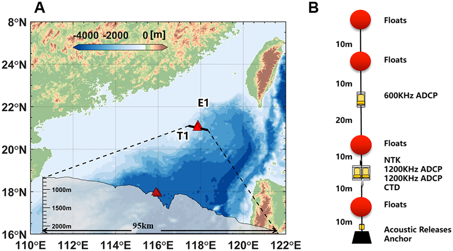
(A)Bathymetry of the northern SCS from the 15 arc-second General Bathymetric Chart of the Oceans (GEBCO) dataset. The red triangles show the mooring locations. (B) Schematic of the mooring at T1.
The downward-looking 1200 kHz ADCP had a blanking distance of 0.44 m, with a vertical bin size of 2 cm, covering 255 layers at a sampling frequency of 1 s. The downward-looking 600 kHz ADCP had a blanking distance of 0.88 m, a vertical bin size of 50 cm, and 150 measured layers (Table 1). The 20° beam angle of the ADCP transducers effectively avoided acoustic interference between the 600 kHz ADCP and 1200 kHz ADCPs mounted below. Its observational range fully covered that of the 1200 kHz ADCP, providing a background current field for collaborative observations of turbulent mixing. Due to the influence of echoes within a range of about 15m from the bottom of the sea, not all observation layers are used for calculations.
Table 1
| Instrument | Depth [m] | Orientation | Water mode | Bin size [cm] | Bin number | Internal [s] | Ensembles/ Burst duration |
|---|---|---|---|---|---|---|---|
| 600 kHz ADCP | 1033 | Down | / | 50 | 150 | 30 | 20/1h |
| NTK | 1063 | / | / | / | / | 10 | / |
| 1200 kHz ADCP-1 | 1064 | Down | 12 | 2 | 255 | 1 | 1800/2h |
| 1200 kHz ADCP-2 | 1064 | Down | 11 | 2 | 255 | 1 | 1800/2h |
The configuration information for mooring.
The ADCP datasets underwent quality control procedures prior to turbulence estimation. During background flow processing, invalid velocity measurements across all bins were eliminated based on echo intensity and correlation thresholds. Subsequent despiking was performed on raw beam velocities using a 3σ criterion. These data were then transformed from beam coordinates to Earth coordinates utilizing recorded instrument attitude parameters. Valid velocities were vertically interpolated onto standardized depth levels. The near-bottom deployment with sufficient buoyancy maintained taut mooring lines, effectively suppressing tilt-induced artifacts during short-term observations. Therefore, for the calculation of turbulent fluctuations, raw velocities in beam coordinates were preserved and used without interpolation to standard depths.
2.2 Estimation of turbulent dissipation rates
Based on the assumption of fully developed isotropic turbulence, four methods are used to estimate the turbulent dissipation rates, ɛ. The fluctuation of velocity u’ is obtained by subtracting the Reynolds-averaged velocity from the original velocity (Tennekes and Lumley, 1972). The separation of time scales is selected such that, over the averaging interval, the mean flow is statistically stationary, and . The overbar denotes an average, while the prime represents the fluctuation from the mean. Tests with averaging windows from 10 s to 30 min showed that intervals that were too short or too long introduced significant biases, whereas 40 s, 60 s, and 80 s windows produced nearly identical dissipation estimates. Thus, 60 s was adopted as an optimal compromise between accuracy and stability.
2.2.1 Second-order structure function method
Structure functions are used to quantify the statistical properties of turbulence (Kolmogorov, 1941). The longitudinal second-order structure function is described as the correlation of fluctuation velocity between two points separated by a close distance r, which refers to the spatial separation between two measurement points along an ADCP beam within a single profile:
where is the fluctuation of velocity as a function of space z and space separation r. The relationship between the second-order structure functions and the turbulent dissipation rate and the space separation r is described as:
where is a universal constant (Kolmogorov, 1941).
High-resolution ADCP measurements provide vertical velocity profiles, enabling the calculation of structure functions for estimating ɛ (Wiles et al., 2006; Lorke, 2007; Lucas et al., 2014; McMillan and Hay, 2017). As the noise is uncorrelated with the signal, the second-order structure function obtained by ADCPs is described as:
where denotes the error introduced by noise (McMillan and Hay, 2017), is the turbulent dissipation rate. According to Kolmogorov’s theory, α is expected to be 2/3 in the inertial subrange. Based on the above relationship, is obtained by least squares fitting of the second-order structure function. For the 1200 kHz ADCP measurements, we evaluated for separation distances r less than 0.84 m (42 layers from layer 1). Assuming isotropy, is calculated by averaging results from the four beams all four methods in this paper.
2.2.2 Inertial subrange wavenumber spectral method
The spectral form of the two-thirds law was obtained independently (Obukhov, 1941) which gives the familiar -5/3 dependence of the turbulent velocity spectral density on the wavenumber k in the inertial subrange. The inertial subrange of velocity spectrum is described as:
where is a universal constant, represents the wavenumber. Assuming that the noise is uncorrelated with the true signal, the inertial subrange of observed wavenumber spectrum is described as:
where denotes the noise introduced by measurement errors (McMillan and Hay, 2017). The noise level is obtained by averaging the spectral floor, which appears as the high-wavenumber plateau in the observed velocity spectra, typically caused by electronic and Doppler noise (van Haren et al., 1994; Hay et al., 2013). Then was estimated by iterative integral of the along-beam velocity spectral densities within the inertial subrange. Each profile consists of 150 measurements with a vertical spacing of , yielding a total extent of . The resolvable wavenumber range is therefore to the Nyquist wavenumber . The integration lower limit of 2 cpm following practice in microstructure turbulence analyses (e.g., Oakey, 1982; Bluteau et al., 2011), and it exceeds the theoretical lower wavenumber limit of the inertial subrange corresponding to the current dissipation rate intensity (W/kg). The upper limit of the integration domain was gradually increased until the difference between the integrated observed spectrum and the theoretical form reached a minimum. Meanwhile, the upper limit was further constrained to remain below the Kolmogorov wavenumber .
2.2.3 Inertial subrange frequency spectral method
Due to the challenge of obtaining high spatial resolution velocity measurement, estimation of ɛ often relies on single-point time series with the Taylor’s frozen-turbulence hypothesis (Lorke and Wüest, 2005; McMillan et al., 2016; McMillan and Hay, 2017). The Taylor frozen-turbulence hypothesis proposes that the turbulent eddy in a flow does not change significantly as they move downstream past a fixed observation point, as if they were frozen in time (Taylor, 1938). The corresponding mathematical expression of the hypothesis is
where represents space location, represents the time delay, the represents the constant convection velocity. In one dimension, the spectra described as:
where represents the wavenumber, and represents the frequency. Following the relationship:
the noise is estimated by computing the average the spectral floor, and is estimated by iterative integral of the along-beam velocity spectral densities within the inertial subrange. The iterative process follows the approach described in Section 2.2.2.
2.2.4 Elliptic approximation model
The EAM, proposed by He and Zhang (2006), was initially devised for analyzing the velocity space-time correlation function in turbulent shear flows. The Taylor hypothesis links spatiotemporal scales through a linear relationship, thereby eliminating the temporal dimension from spatiotemporal correlations. In practice, devices measuring turbulent fluctuations require a rapid response time to ensure that the probe samples undisturbed fluid. Additionally, the platform’s speed must be carefully controlled. It should neither be too fast nor too slow to precisely capture the structure of turbulent eddies. However, the Taylor frozen-turbulence hypothesis fails in cases where variations in advection past the sensor occur within the short duration allocated for spectrum calculation. Under such circumstances, the EAM offers a more appropriate framework for characterizing spatiotemporal correlations:
where R is the correlation function as a function of space separation z and time delay τ, the convective velocity characterizes the convection of currents, and the sweeping velocity V characterizes the distortion of currents which is related to sweeping hypothesis of Kraichnan (1964). Employing characteristic velocities and , this method produces an elliptical depiction of the iso-correlation contours in the z-τ plane.
For or close to 0, a length scale and a time scale are defined which gives the equivalence between the space and time domain (Fer et al., 2014; Wallace, 2014; He et al., 2015),
It can be Fourier transformed into the wavenumber and frequency space,
The correlation across space and time can be represented via spatial correlations, denoted as alongside U and V, which collectively satisfy the relation (He and Zhang, 2006; He and Tong, 2009; He et al., 2010):
Fulfilling the EAM allows for the determination of time scale constant and spatial scale constant , and facilitating the conversion of time spectra to spatial energy spectra (Fer et al., 2014; He et al., 2015),
Further determination of ɛ is achieved through,
where the noise is estimated by computing the average the spectral floor, and is estimated by iterative integral of the along-beam velocity spectral densities within the inertial subrange.
3 Results of estimation of turbulent dissipation rates
3.1 Configuration comparative experiments
Effective configurations of water mode, bin size, sampling frequency, ambiguous velocity and number of bins of 1200 kHz ADCPs contribute to diminishing measurement errors. To elucidate the influence of different configurations and to determine the optimal setup, a series of experiments were conducted at S1 (Table 1).
Experiments S108, S112, and S107, were configured with different bin sizes (5cm, 2cm, and 1cm, respectively). We used ISM-k and SFM to analyze the experimental data and compare results. As shown in Table 2, a smaller bin size results in a smaller noise introduced by measurement errors (N), but it also leads to a larger standard deviation. When analyzed using ISM-K, N is the smallest in S107 (W/kg).
Table 2
| Experiment | Bin size [cm] | Bin number | Internal [s] | Ensembles/ Burst duration | LOG10 () MEAN [W/kg] | LOG10 (ɛ) STD [W/kg] | LOG10 (N) MEAN [W/kg] |
|---|---|---|---|---|---|---|---|
| S102 | 25 | 120 | 4 | 60/10min | -7.76 | 0.32 | -5.68 |
| S104 | 1 | 120 | 1 | 600/10min | -8.03 | 0.31 | -5.63 |
| S107 | 1 | 200 | 1 | 600/10min | -8.69 | 0.51 | -5.72 |
| S108 | 5 | 255 | 1 | 600/10min | -8.23 | 0.30 | -5.21 |
| S112 | 2 | 160 | 1 | 1800/30min | -7.41 | 0.57 | -5.32 |
| S120 | 2 | 255 | 0.5 | 300/10min | -7.45 | 0.32 | -4.26 |
The deployment information and results of experiments at S1 with different settings.
In experiments S102, S107, and S120, which feature varying sampling frequencies (0.25 Hz, 1 Hz, and 2 Hz respectively), a higher temporal resolution is beneficial for reducing errors in ɛ estimation despite slightly increasing velocity observation error. Reducing the sampling interval improves the ability to meet turbulence measurement standards. However, data from S120 indicate that the instrument cannot calculate uniformly spaced samples when the sampling interval is less than 1 second.
The number of bins directly affects the algorithm’s processing speed and the standard deviation of the measurements, particularly in bins farther from the instrument. A balance between coverage and resolution is assessed by comparing S104 and S107; the selection of a limited number of bins was found not to significantly impact observation quality, with the noise level of ~ and ~ , respectively. To maximize data collection, selecting a larger number of bins is recommended. In addition to configurations mentioned above, the threshold of the correlation value, which is commonly set to a default value of 64, is recommended to be set to zero in the deep ocean.
3.2 Elliptic approximation model
In Taylor’s model, decorrelation is determined solely by the convection velocity caused by mean flows. He and Zhang (2006) theorized that EAM could precisely map out the areas of correlation over a broad range of z and τ, a feature ascribed to the inherent self-similarity of the flow (He et al., 2010). This theory was validated through the analysis of numerical simulations (Zhao and He, 2009; Wallace, 2014; He et al., 2015) and experimental investigations (Zhou et al., 2011; Hogg and Ahlers, 2013; Wang et al., 2014).
The EAM has been examined in the upper ocean (Liang et al., 2024). Here, we apply the EAM to in situ deep oceanographic observations. Using velocity data from a 1200 kHz ADCP, the spatiotemporal correlation function was computed, yielding correlation coefficients that exhibit unimodal distributions in both the spatial and temporal dimensions. The correlation peaks at the origin (r = 0, τ = 0) and decays progressively with increasing spatial lag r and temporal lag τ (Figure 2A). If the Taylor’s frozen turbulence hypothesis were well valid in this turbulent regime, the spatiotemporal correlation structure would degenerate into a straight line. However, the observed contours clearly form elliptical patterns, closely matching the theoretical ellipses predicted by the EAM. As an example, the spatiotemporal correlation field was computed using a 1-minute velocity time series from 05:30 to 05:31 on August 1, with the 80th vertical bin as the origin, spanning 160 adjacent vertical bins. Characteristic variables U and V were employed to further validate the EAM by examining the functional relationship between r, τ, and the correlation coefficients. The correlation curves of velocity versus time lag for different spatial internals first increase to a peak and then decay, all exhibiting unimodal behavior. Symmetry degrades with increasing r (Figure 2B). The temporal correlation functions derived from observations agree well with the theoretical correlation curves defined by the EAM when r< 1 m (Figure 2C), indicating that the model is valid within a finite spatial extent.
Figure 2
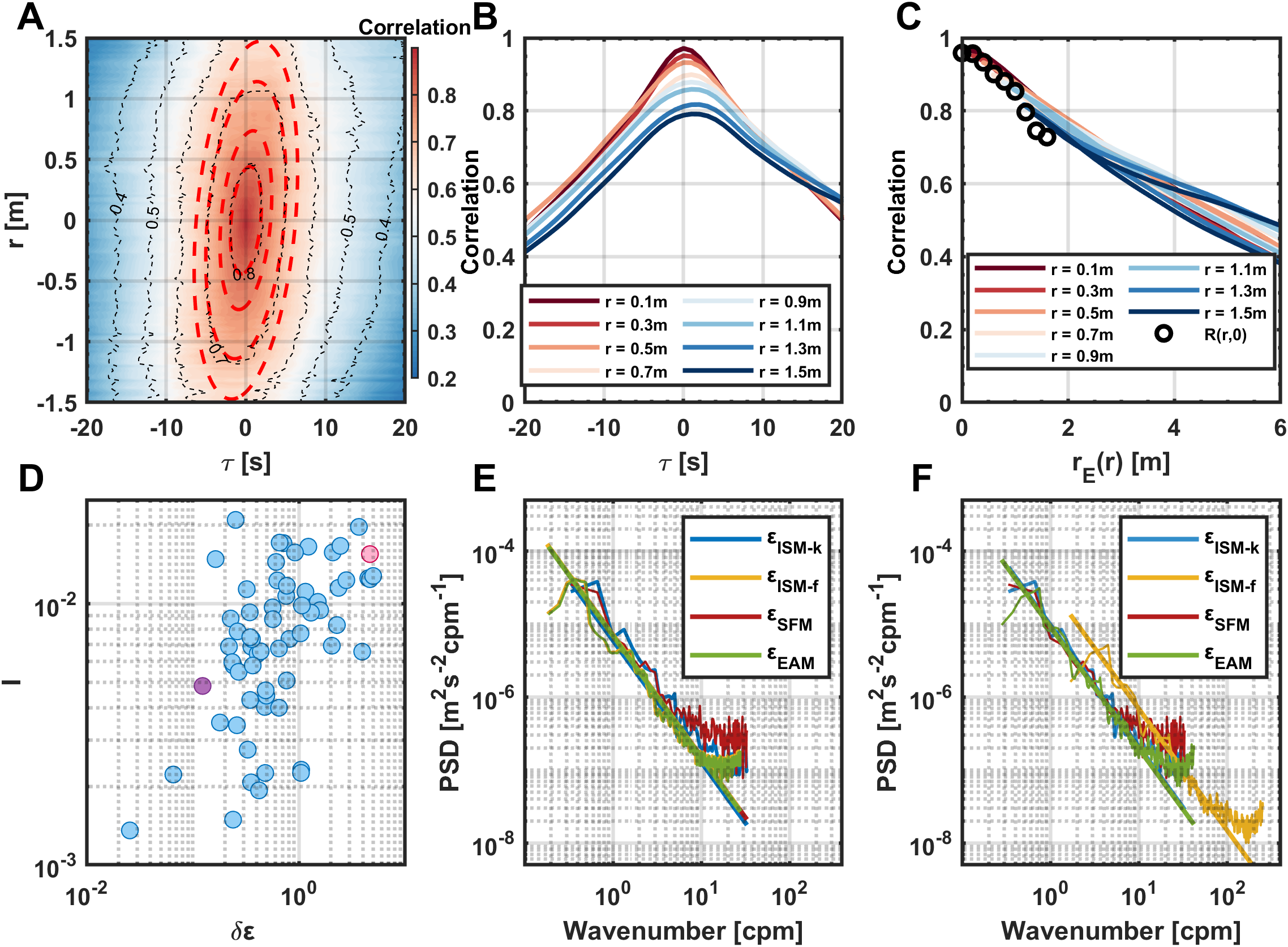
(A) Temporal and spatial correlation coefficients. The red dashed lines represent the theoretical ellipses obtained by EAM. (B) The relationship between and τ at different spatial intervals. (C) The relationship between different and at different spatial intervals. (D)δɛ is the difference between the ɛ calculated by ISM-f and the calculated by ISM-k and SFM, defined as . The turbulence intensity (I) is the ratio between the root-mean-square of the turbulent velocity and the time-averaged velocity. (E) Spectra calculated by the four methods corresponding to the purple points in (D, F) Spectra calculated by the four methods corresponding to the pink point in (D).
Turbulence intensity (I) is commonly used to quantify the strength of turbulence and is defined as the ratio of the root-mean-square (RMS) of velocity fluctuations to the mean flow velocity. In this study, the mean dissipation rates obtained from the SFM and ISM-k methods were taken as reference values, and the relative error δɛ was defined as the difference between the dissipation rate estimated by the ISM-f method and, normalized by . Results indicate that the estimation error increases with rising I (Figure 2D), implying that the Taylor frozen-turbulence hypothesis tends to break down under strong turbulence conditions in our observation, although it still meet the range required by the classical Taylor freezing assumption in terms of I. To further compare the performance of different estimation methods, the function of SFM was transformed into the spectral domain via Fourier transform. In comparison to the spectrum derived from ISM-f under the Taylor frozen-turbulence hypothesis, the results from the EAM show better agreement with those from ISM-k and SFM in this context (Figures 2E, F). These findings demonstrate the effectiveness of the EAM in accurately converting measurements from the time domain to the spatial domain. Furthermore, grounded in a robust spatiotemporal transformation framework, this method is not only applicable to 1200 kHz ADCP-based velocity measurements for ɛ estimation, but can also be extended to other high-frequency, time-continuous datasets with at least two spatially adjacent (within 1 m) velocity records, thereby enhancing the applicability and data utilization efficiency in ocean turbulence observation.
4 Variability of turbulent dissipation rates
Turbulence measurements require a high sampling resolution. To attain a robust observation of turbulence, the initial objective is to ensure that high-resolution sampling provides fundamentally stable and effective measurements of current velocity. In conjunction with more established single-point current meter NTK, ADCP velocity observations are utilized to assess the feasibility of employing high-resolution ADCP for deep-sea current observations. The observation results from 1200kHz ADCP and 600kHz ADCP show good consistency with the velocity observed by NTK (Figure 3).
Figure 3
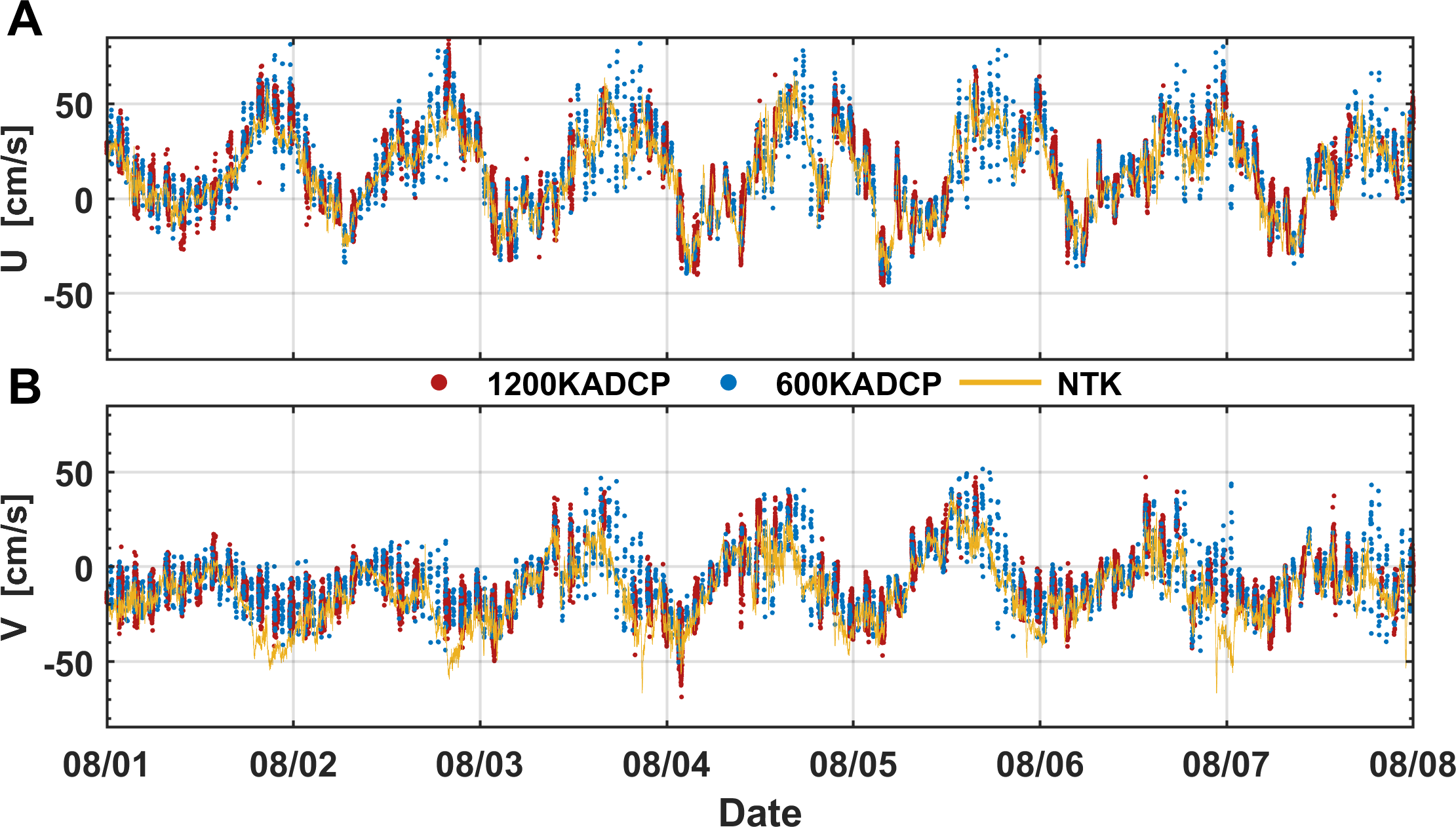
(A) The meridional and (B) zonal current velocities measured by the 1200 kHz ADCP (red points), 600 kHz ADCP (blue points), and acoustic current meter Nortek Aquadopp DW at similar depths (yellow lines).
The time series of ɛ derived from SFM, ISM-k, and EAM at T1 demonstrate excellent consistency with each other as shown in Figure 4. The average of results from these three methods (SFM, ISM-k, EAM) was taken as the observed value of ɛ. Throughout the observation period, the mean ɛ was W/kg. During the seven days of continuous observations, the two-hour resolution time series shows ɛ values ranging from W/kg to W/kg. Within each single day, ɛ can vary by up to two orders of magnitude. For instance, the minimum ɛ observed in 2 August is W/kg, but it reaches as high as W/kg, indicating a 143% increase within the period of just 24 hours. This result suggests that a single profiler measurement is by far not sufficient to capture the full structure of turbulent mixing in the deep ocean, and continuous observations are therefore necessary in order to obtain reliable ɛ measurements.
Figure 4
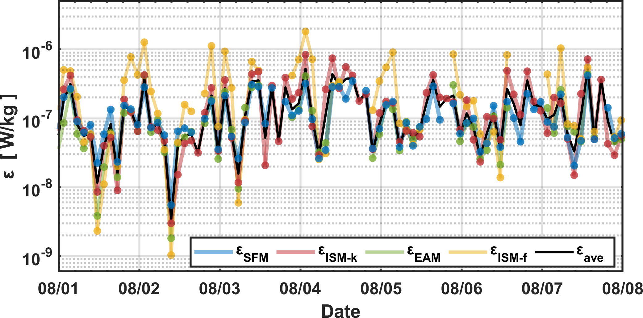
Time series of ɛ obtained by SFM (blue), ISM-k (red), EAM (green), ISM-f (yellow), and the average of the first three methods (black) at T1, with asterisks indicating 30-minute burst averages.
The Richardson number (Ri), defined as , is a predictor of shear instabilities, where is the buoyancy frequency and represents the shear of horizontal velocity (Howard, 1961; Miles, 1961). During the observation period, the temporal variability of mixing intensity matches well with Ri (r = 0.8), indicating that the enhanced mixing could be associated with the decrease in Ri (Figure 5). This suggests that local turbulent dissipation is intensified by pronounced shear instability in the background flow.
Figure 5
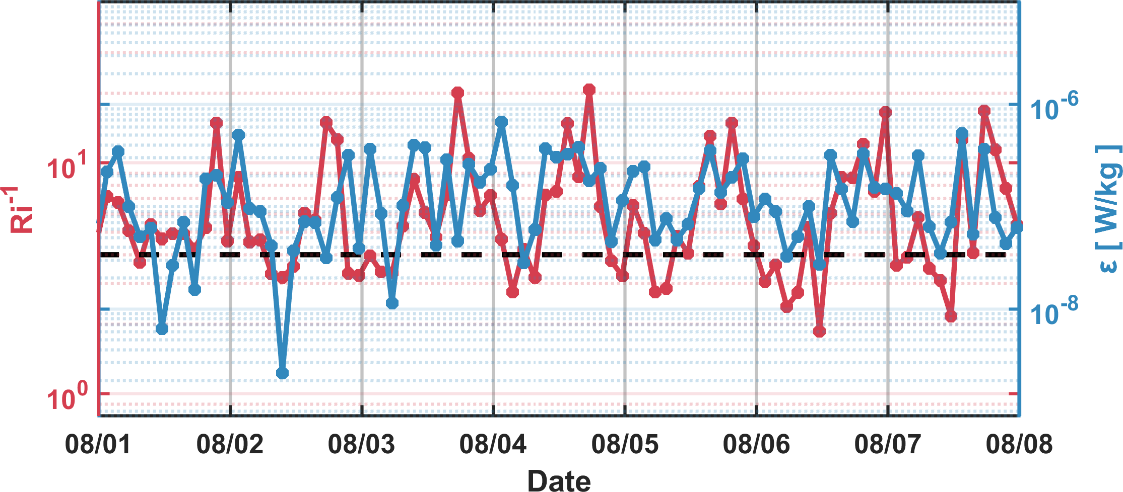
The turbulent kinetic energy dissipation rate averaged across all methods (blue), and the time series of Ri-1 (red). The black dashed line marks the value 4 of Ri-1 (Ri = 0.25).
Dissipation of internal tides is the primary mechanisms for generating shear instability and inducing deep ocean mixing (Shang et al., 2017). Spectral analysis of the horizontal velocity at station E1, a twin mooring located 10 km from T1, reveals distinct peaks corresponding to the diurnal and semi-diurnal tides. The topographic spectrum suggests that this location is conducive to the generation of high-mode internal tides (Figure 6), which is likely responsible for the variations of ɛ. Moreover, this location is also characterized by strong internal tides propagating from in the Luzon Strait (Zhao et al., 2014).
Figure 6
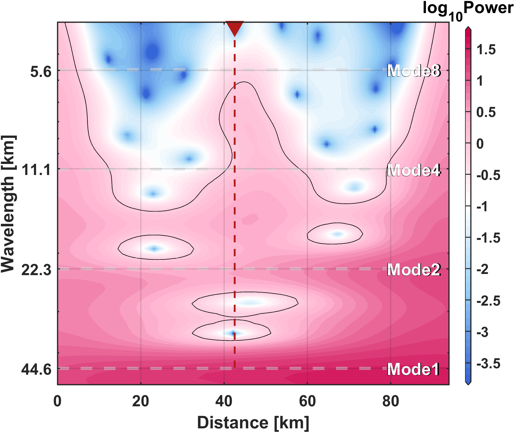
The wavelet spectrum of multibeam bathymetric data in Figure 1A. The red triangle and dashed line represent the location of station T1.
To investigate how these processes influence ɛ, a band-pass filtering was performed to calculate the correlation between changes in ɛ and kinetic energy at different frequencies (Figure 7A). The correlation is notably high in the diurnal band (r = 0.5, Figure 7B), but is negligible on the semi-diurnal frequencies. This result suggests that the dissipation of diurnal internal tides dominate the variability of ɛ. Significant temporal variability in turbulent mixing has also been reported on the northern continental shelf of the SCS (e.g., Huang et al., 2021; Qu et al., 2021; Zhu et al., 2024), with elevated mixing levels attributed to critical interactions between semidiurnal tides and slope topography. These findings further support the necessity of continuous long-term deep-ocean observations to capture the mechanisms linking internal tides to highly intermittent turbulent mixing.
Figure 7
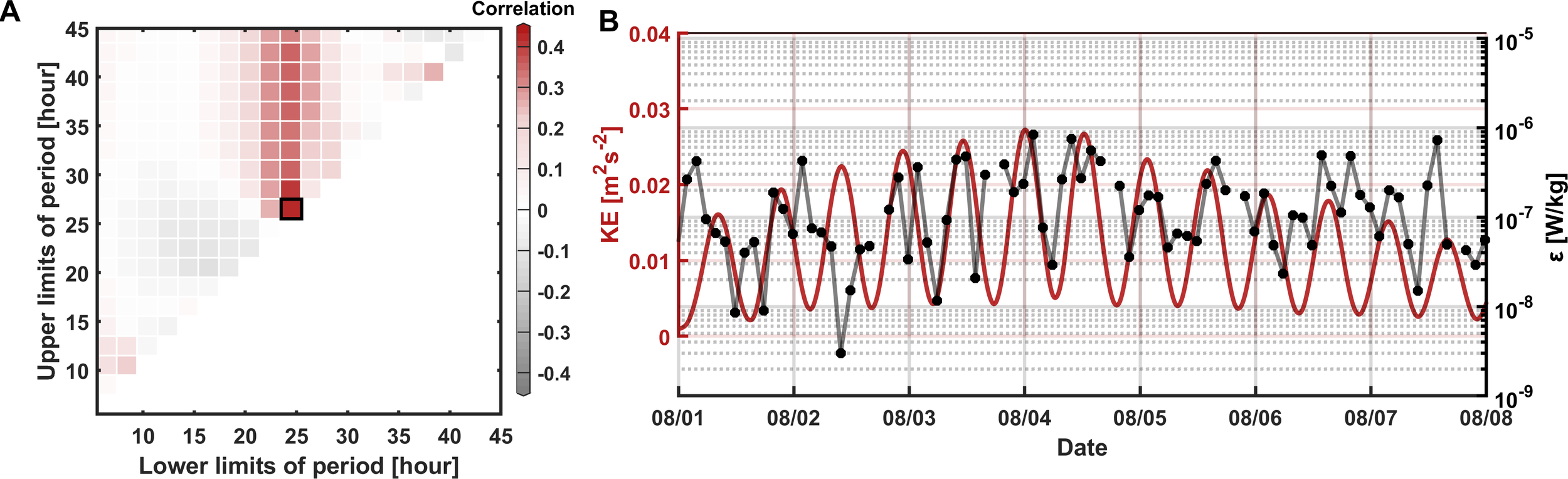
(A) Correlation between ɛ and kinetic energy obtained from horizontal velocities filtered by different time scales. (B) Diurnal kinetic energy (red line) and averaged ɛ (black dotted line) in the time range of the black box in (A).
To examine the influence of internal tides on turbulent mixing variability, modal decomposition was performed for the full-depth current velocity at station E1. Modes 1 and 2, accounting for an average of 69% of total kinetic energy, show low correlation with ɛ (r<0.2) (Figure 8A), while the energy of diurnal internal tides in modes 3–10 exhibits a higher correlation with ɛ (up to 0.5) (Figure 8B). The temporal variability of ɛ is closely related to the local shear instability, which is dominated by the dissipation of high-mode diurnal internal tide. Other multiscale dynamic processes, such as mesoscale eddies (Zhang et al., 2016) and near-inertial waves (Zheng et al., 2023), which extend from the surface to the near-bottom, may also contribute to the variability of ɛ in the deep South China Sea. Their relationships with ɛ will be examined in a future study over the extended observation period.
Figure 8
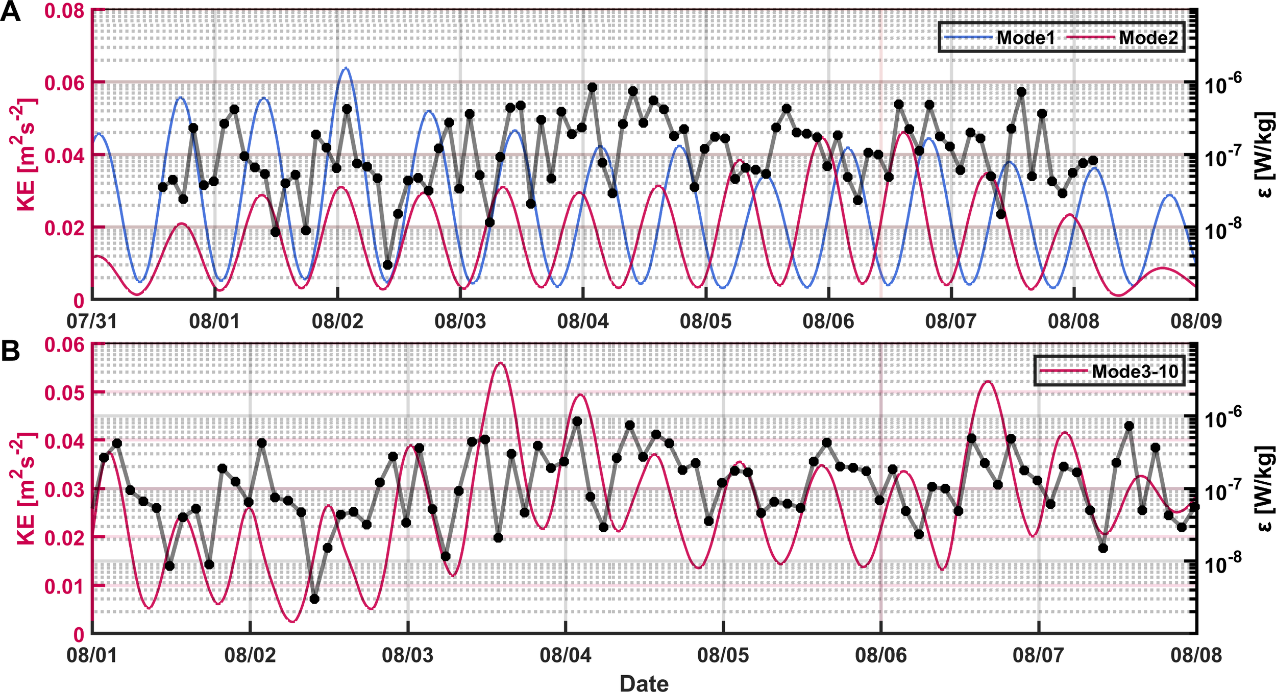
(A) Energy of modes 1 and 2 of the inertial tidal velocity decomposition at E1 and ɛ (black dotted line) (B) Energy of mode 3–10 of the tidal velocity decomposition at E1and averaged ɛ (black dotted line).
5 Conclusions
By conducting a set of mooring experiments in the northeastern South China Sea, we present, for the first time, the efficacy of the 1200 kHz ADCPs for continuous observations of turbulent mixing with high spatial (2cm) and temporal (1Hz) resolution in the deep ocean. Velocity profiles observed by the 1200 kHz ADCPs enable direct estimation of near-bottom dissipation rates using ISM-k and SFM without relying on Taylor’s frozen-turbulence hypothesis. We also test the EAM, which overcomes the limitations of profiling measurements and allows for continuous observations of turbulent mixing in deep ocean through high-frequency current measurements.
Continuous observations of turbulence unveil significant temporal variability in the northeastern South China Sea. With pronounced intermittency, the near bottom dissipation rates, ɛ, can change by up to two orders of magnitude in a single day. The variability of ɛ is closely correlated (r = 0.8) to Ri, which indicates the occurrence of shear instability. Further analysis of the background flow reveals that locally generated diurnal and high-mode internal tides are critical factors influencing the mixing variability. However, the variability of ɛ may also be influenced by other multiscale dynamic processes, whose roles will be explored in future investigations based on extended observation periods. The capability of the 1200 kHz ADCPs for remote current measurements and long-term deployment (months to years) make them suitable for characterizing current velocity across various timescales and investigating the turbulence in the deep ocean.
This study refines observation strategies and achieves continuous observations of turbulence in the deep South China Sea, underscoring the substantial variability of turbulence and the necessity for sustained observations. Further observations are necessary to access the full spectra of variability of turbulent mixing and associated dynamic processes in the deep ocean. The enhanced observational capability of the deep bottom boundary layer turbulent mixing holds significant potential for advancing the understanding of boundary layer dynamics and multiscale energy cascades.
Statements
Data availability statement
The original contributions presented in the study are included in the article/supplementary material, further inquiries can be directed to the corresponding author/s.
Author contributions
HX: Conceptualization, Methodology, Writing – original draft, Formal Analysis, Data curation. CZ: Project administration, Funding acquisition, Conceptualization, Writing – review & editing, Methodology, Formal Analysis. XX: Conceptualization, Data curation, Methodology, Writing – original draft, Formal Analysis. SG: Conceptualization, Writing – review & editing. XH: Writing – review & editing, Conceptualization. TQ: Writing – review & editing, Conceptualization. WZ: Conceptualization, Writing – review & editing. JT: Writing – review & editing, Conceptualization.
Funding
The author(s) declare that financial support was received for the research and/or publication of this article. This study was supported by the National Natural Science Foundation of China (Grants 92258301, 42076027, 91958205, 91858203), the “Taishan” Talents Program (Grant tsqn202306094) and the China Postdoctoral Science Foundation (Grant 2024M763111).
Acknowledgments
We acknowledge the support from the NSFC Shiptime Sharing Project (Grants 42049905, 42249905, 42349905) for the cruises NORC2021-05, NORC2023-05, and NORC2024-05. Special thanks to the crew of the R/V Dongfanghong 3 for their support during the expeditions. Additionally, we thank Dr. Jinhan Xie of the Peking University for helpful discussions on an earlier version of this manuscript.
Conflict of interest
The authors declare that the research was conducted in the absence of any commercial or financial relationships that could be constructed as a potential conflict of interest.
Generative AI statement
The author(s) declare that no Generative AI was used in the creation of this manuscript.
Any alternative text (alt text) provided alongside figures in this article has been generated by Frontiers with the support of artificial intelligence and reasonable efforts have been made to ensure accuracy, including review by the authors wherever possible. If you identify any issues, please contact us.
Publisher’s note
All claims expressed in this article are solely those of the authors and do not necessarily represent those of their affiliated organizations, or those of the publisher, the editors and the reviewers. Any product that may be evaluated in this article, or claim that may be made by its manufacturer, is not guaranteed or endorsed by the publisher.
References
1
Alford M. H. Girton J. B. Voet G. Carter G. S. Mickett J. B. Klymak J. M. (2013). Turbulent mixing and hydraulic control of abyssal water in the Samoan Passage. Geophysical Res. Lett.40, 4668–4674. doi: 10.1002/grl.50684
2
Alford M. H. Wynne-Cattanach B. Le Boyer A. Couto N. Voet G. Spingys C. P. et al . (2025). Buoyancy flux and mixing efficiency from direct, near-bottom turbulence measurements in a submarine canyon. J. Phys. Oceanography. 55(2), 97–118. doi: 10.1175/JPO-D-24-0005.1
3
Bluteau C. E. Jones N. L. Ivey G. N. (2011). Estimating turbulent kinetic energy dissipation using the inertial subrange method in environmental flows. Limnology Ocean Methods9(7), 302–321. doi: 10.4319/lom.2011.9.302
4
Fer I. Peterson A. K. Ullgren J. E. (2014). Microstructure measurements from an underwater glider in the turbulent Faroe Bank Channel overflow. J. Atmospheric Oceanic Technol.31, 1128–1150. doi: 10.1175/JTECH-D-15-0218.1
5
Ferrari R. (2014). What goes down must come up. Nature513, 179–180. doi: 10.1038/513179a
6
Ferris L. Gong D. Merrifield S. St. Laurent L. C. (2022). Contamination of finescale strain estimates of turbulent kinetic energy dissipation by frontal physics. J. Atmospheric Oceanic Technol.39, 619–640. doi: 10.1175/jtech-d-21-0088.1
7
Gargett A. E. (1988). A “large-eddy” approach to acoustic remote sensing of turbulent kinetic energy dissipation rate ɛ. Atmosphere-Ocean26, 483–508. doi: 10.1080/07055900.1988.9649314
8
Gregg M. C. (1991). The study of mixing in the ocean: A brief history. Oceanography4, 39–45. doi: 10.5670/oceanog.1991.21
9
Hay A. E. McMillan J. M. Cheel R. Schillinger D. (2013). Turbulence and drag in a high reynolds number tidal passage targetted for in-stream tidal power. IEEE. (San Diego). doi: 10.23919/OCEANS.2013.6741193
10
He G. Zhang J. (2006). Elliptic model for space-time correlations in turbulent shear flows. Phys. Rev. E73(5), 055303. doi: 10.1103/PhysRevE.73.055303
11
He X. He G. Tong P. (2010). Small-scale turbulent fluctuations beyond Taylor’s frozen-flow hypothesis. Phys. Rev. E81, 65303. doi: 10.1103/PhysRevE.81.065303
12
He X. Tong P. (2009). Measurements of the thermal dissipation field in turbulent Rayleigh-Bénard convection. Phys. Rev. E79, 26306. doi: 10.1103/PhysRevE.79.026306
13
He X. van Gils D. P. M. Bodenschatz E. Ahlers G. (2015). Reynolds numbers and the elliptic approximation near the ultimate state of turbulent Rayleigh–Bénard convection. New J. Phys.17, 63028. doi: 10.1088/1367-2630/17/6/063028
14
Hogg J. Ahlers G. (2013). Reynolds-number measurements for low-Prandtl-number turbulent convection of large-aspect-ratio samples. J. Fluid Mechanics725, 664–680. doi: 10.1017/jfm.2013.179
15
Howard L. N. (1961). Note on a paper of john W. Miles. J. Fluid Mechanics10, 509–512. doi: 10.1017/S0022112061000317
16
Huang P. Cen X. Guo S. Lu Y. Zhou S. Qiu X. et al . (2021). Variance of bottom water temperature at the continental margin of the northern south China sea. J. Geophysical Research: Oceans126(2), e2020JC015843. doi: 10.1029/2019jc015843
17
Huang X. Chen Z. Zhao W. Zhang Z. Zhou C. Yang Q. et al . (2016). An extreme internal solitary wave event observed in the northern South China Sea. Sci. Rep.6, 30041. doi: 10.1038/srep30041
18
Hughes K. G. Moum J. N. Shroyer E. L. (2020). Heat transport through diurnal warm layers. J. Phys. Oceanography50, 2885–2905. doi: 10.1175/JPO-D-20-0079.1
19
Hummels R. Dengler M. Rath W. Foltz G. R. Schütte F. Fischer T. et al . (2020). Surface cooling caused by rare but intense near-inertial wave induced mixing in the tropical Atlantic. Nat. Commun.11(1), 3829. doi: 10.1038/s41467-020-17601-x
20
Jochum M. Briegleb B. P. Danabasoglu G. Large W. G. Norton N. J. Jayne S. R. et al . (2013). The impact of oceanic near-inertial waves on climate. J. Climate26, 2833–2844. doi: 10.1175/jcli-d-12-00181.1
21
Kolmogorov A. N. (1941). Dissipation of energy in locally isotropic turbulence. Doklady Akademii Nauk SSSR32, 16–18.
22
Kraichnan R. H. (1964). Kolmogorov’s hypotheses and eulerian turbulence theory. Phys. Fluids7, 1723–1734. doi: 10.1063/1.2746572
23
Ledwell J. R. Montgomery E. T. Polzin K. L. St. Laurent L. C. Schmitt R. W. Toole J. M. (2000). Evidence for enhanced mixing over rough topography in the abyssal ocean. Nature403, 179–182. doi: 10.1038/35003164
24
Levine E. R. Lueck R. G. (1999). Turbulence measurement from an autonomous underwater vehicle. J. Atmospheric Oceanic Technol.16, 1533–1544. doi: 10.1175/1520-0426(1999)016<1533:TMFAAU>2.0.CO;2
25
Li J. Yang Q. Sun H. Zhao W. Tian J. (2022). Spatial variation of bottom mixed layer in the South China Sea and a potential mechanism. Prog. Oceanogr.206. doi: 10.1016/j.pocean.2022.102856
26
Liang C. Shang X. Chen G. He X. Tong P. (2024). Application of the EA model to the velocity transversal space-time cross-correlation functions measured in the ocean. Acta Mechanica Sin.40, 323381. doi: 10.1007/s10409-023-23381-x
27
Lien R.-C. Sanford T. B. Carlson J. A. Dunlap J. H. (2016). Autonomous microstructure EM-APEX floats. Methods Oceanography17, 282–295. doi: 10.1016/j.mio.2016.09.003
28
Liu Z. Lozovatsky I. (2012). Upper pycnocline turbulence in the northern South China Sea. Chin. Sci. Bull.57, 2302–2306. doi: 10.1007/s11434-012-5137-8
29
Lohrmann A. Hackett B. Røed L. P. (1990). High resolution measurements of turbulence, velocity and stress using a pulse-to-pulse coherent sonar. J. Atmospheric Oceanic Technol.7, 19–37. doi: 10.1175/1520-0426(1990)007<0019:HRMOTV>2.0.CO;2
30
Lorke A. (2007). Boundary mixing in the thermocline of a large lake. J. Geophysical Res.112(C9), 019. doi: 10.1029/2006jc004008
31
Lorke A. Wüest A. (2005). Application of coherent ADCP for turbulence measurements in the bottom boundary layer. J. Atmospheric Oceanic Technol.22, 1821–1828. doi: 10.1175/JTECH1813.1
32
Lu Y. Lueck R. G. (1999). Using a broadband ADCP in a tidal channel. Part II: Turbulence. J. Atmospheric Oceanic Technol.16, 1568–1579. doi: 10.1175/1520-0426(1999)016<1568:UABAIA>2.0.CO;2
33
Lucas N. S. Simpson J. H. Rippeth T. P. Old C. P. (2014). Measuring turbulent dissipation using a tethered ADCP. J. Atmospheric Oceanic Technol.31, 1826–1837. doi: 10.1175/jtech-d-13-00198.1
34
Lueck R. G. (2022). The statistics of oceanic turbulence measurements. Part I: shear variance and dissipation rates. J. Atmospheric Oceanic Technol.39, 1259–1271. doi: 10.1175/jtech-d-21-0051.1
35
Lueck R. Wolk F. Yamazaki H. (2002). Oceanic velocity microstructure measurements in the 20th century. J. Oceanography58, 153–174. doi: 10.1023/A:1015837020019
36
Marshall J. Speer K. (2012). Closure of the meridional overturning circulation through Southern Ocean upwelling. Nat. Geosci.5, 171–180. doi: 10.1038/NGEO1391
37
McDougall T. J. Ferrari R. (2017). Abyssal upwelling and downwelling driven by near-boundary mixing. J. Phys. Oceanography47, 261–283. doi: 10.1175/jpo-d-16-0082.1
38
McMillan J. M. Hay A. E. (2017). Spectral and structure function estimates of turbulence dissipation rates in a high-flow tidal channel using broadband ADCPs. J. Atmospheric Oceanic Technol.34, 5–20. doi: 10.1175/jtech-d-16-0131.1
39
McMillan J. M. Hay A. E. Lueck R. G. Wolk F. (2016). Rates of dissipation of turbulent kinetic energy in a high reynolds number tidal channel. J. Atmospheric Oceanic Technol.33, 817–837. doi: 10.1175/jtech-d-15-0167.1
40
Meredith M. Garabato A. N. (2021). Ocean mixing: Drivers, mechanisms and impacts (Amsterdam: Elsevier).
41
Miles J. W. (1961). On the stability of heterogeneous shear flows. J. Fluid Mechanics10, 496–508. doi: 10.1017/S0022112061000305
42
Miller U. K. Zappa C. J. Zippel S. F. Farrar J. T. Weller R. A. (2022). Scaling of moored surface ocean turbulence measurements in the southeast pacific ocean. J. Geophysical Research: Oceans128(1), e2022JC018901. doi: 10.1029/2022jc018901
43
Moum J. N. Nash J. D. (2009). Mixing measurements on an equatorial ocean mooring. J. Atmospheric Oceanic Technol.26, 317–336. doi: 10.1175/2008JTECHO617.1
44
Moum J. N. Perlin A. Nash J. D. McPhaden M. J. (2013). Seasonal sea surface cooling in the equatorial Pacific cold tongue controlled by ocean mixing. Nature500, 64–67. doi: 10.1038/nature12363
45
Munk W. (1966). Abyssal recipes. Deep Sea Res. Oceanographic Abstracts13, 707–730. doi: 10.1016/0011-7471(66)90602-4
46
Nielson J. R. Henderson S. M. (2022). Bottom boundary layer mixing processes across internal seiche cycles: Dominance of downslope flows. Limnology Oceanography67, 1111–1125. doi: 10.1002/lno.12060
47
Oakey N. S. (1982). Determination of the rate of dissipation of turbulent energy from simultaneous temperature and velocity shear microstructure measurements. J. Phys. Oceanography12, 256–271. doi: 10.1175/1520-0485(1982)012<0256:DOTROD>2.0.CO;2
48
Obukhov A. (1941). On the energy distribution in the spectrum of a turbulent flow. Doklady Akademii Nauk SSSR32, 19–21.
49
Polzin K. L. Toole J. M. Ledwell J. R. Schmitt R. W. (1997). Spatial variability of turbulent mixing in the abyssal ocean. Science276, 93–96. doi: 10.1126/science.276.5309.93
50
Qu L. Lu Y. Cen X. Guo S. Huang P. Yu L. et al . (2021). Temporal variability in bottom water structures of the continental slope in the northern south China sea. J. Geophysical Research: Oceans126(7), e2021JC017177. doi: 10.1029/2021jc017177
51
Rowe F. Young J. (1979). “An ocean current profiler using doppler sonar,” in OCEANS ‘79, Cambridge: MIT press. 292–297.
52
Shang X.-D. Liang C.-R. Chen G.-Y. (2017). Spatial distribution of turbulent mixing in the upper ocean of the South China Sea. Ocean Sci.13, 503–519. doi: 10.5194/os-13-503-2017
53
Stacey M. T. Monismith S. G. Burau J. R. (1999). Measurements of Reynolds stress profiles in unstratified tidal flow. J. Geophysical Research: Oceans104, 10933–10949. doi: 10.1029/1998jc900095
54
St. Laurent L. C. (2008). Turbulent dissipation on the margins of the South China Sea. Geophysical Res. Lett.35(23), L23615. doi: 10.1029/2008gl035520
55
Sun H. Zhao W. Yang Q. Cai S. Liang X. Tian J. (2019). Estimating four-dimensional internal wave spectrum in the northern south China sea. J. Atmospheric Oceanic Technol.36, 1199–1216. doi: 10.1175/jtech-d-18-0046.1
56
Talley L. (2013). Closure of the global overturning circulation through the Indian, pacific, and southern oceans: schematics and transports. Oceanography26, 80–97. doi: 10.5670/oceanog.2013.07
57
Taylor G. I. (1938). The spectrum of turbulence. Proc. R. Soc. London. Ser. A - Math. Phys. Sci.164, 476–490. doi: 10.1098/rspa.1938.0032
58
Tennekes H. Lumley J. L. (1972). A first course in turbulence. Cambridge: MIT press.
59
Thorpe S. A. Osborn T. R. Jackson J. F. E. Hall A. J. Lueck R. G. (2003). Measurements of turbulence in the upper-ocean mixing layer using autosub. J. Phys. Oceanography33, 122–145. doi: 10.1175/1520-0485(2003)033<0122:MOTITU>2.0.CO;2
60
Tian J. Zhao W. Yang Q. (2009). Enhanced diapycnal mixing in the south China sea. J. Phys. Oceanography39, 3191–3203. doi: 10.1175/2009jpo3899.1
61
van Haren H. Oakey N. Garrett C. (1994). Measurements of internal wave band eddy fluxes above a sloping bottom. J. Mar. Res.52(5), 909–946. doi: 10.1357/0022240943076876
62
Wallace J. M. (2014). Space-time correlations in turbulent flow: A review. Theor. Appl. Mechanics Lett.4, 022003. doi: 10.1063/2.1402203
63
Wang W. Guan X.-L. Jiang N. (2014). TRPIV investigation of space-time correlation in turbulent flows over flat and wavy walls. Acta Mechanica Sin.30, 468–479. doi: 10.1007/s10409-014-0060-7
64
Waterhouse A. F. Lee C. M. Sanford T. B. Naveira Garabato A. C. Waterman S. Fer I. et al . (2014). Global patterns of diapycnal mixing from measurements of the turbulent dissipation rate. J. Phys. Oceanography44, 1854–1872. doi: 10.1175/jpo-d-13-0104.1
65
Whalen C. B. de Lavergne C. Naveira Garabato A. C. Klymak J. M. MacKinnon J. A. Sheen K. L. (2020). Internal wave-driven mixing: governing processes and consequences for climate. Nat. Rev. Earth Environ.1, 606–621. doi: 10.1038/s43017-020-0097-z
66
Wiles P. J. Rippeth T. P. Simpson J. H. Hendricks P. J. (2006). A novel technique for measuring the rate of turbulent dissipation in the marine environment. Geophysical Res. Lett.33(21), 608. doi: 10.1029/2006gl027050
67
Wolk F. Lueck R. G. (2002). A new free-fall profiler for measuring biophysical microstructure. doi: 10.1175/1520-0426(2002)019<0780:ANFFPF>2.0.CO;2
68
Wolk F. Lueck R. G. St. Laurent L. C. (2009). “Turbulence measurements from a glider,” in OCEANS 2009 (MS: IEEE, Biloxi), 1–6.
69
Wynne-Cattanach B. L. Couto N. Drake H. F. Ferrari R. Le Boyer A. Mercier H. et al . (2024). Observations of diapycnal upwelling within a sloping submarine canyon. Nature630, 884–890. doi: 10.1038/s41586-024-07411-2
70
Xiao X. Zhou C. Yang Q. Jing Z. Liu Z. Yuan D. et al . (2023). Diapycnal upwelling over the kyushu-Palau ridge in the north pacific ocean. Geophysical Res. Lett.50(18), e2023GL104369. doi: 10.1029/2023gl104369
71
Yang Q. Tian J. Zhao W. Liang X. Zhou L. (2014). Observations of turbulence on the shelf and slope of northern South China Sea. Deep Sea Res. Part I Oceanogr. Res. Pap.87, 43–52. doi: 10.1016/j.dsr.2014.02.006
72
Yang Q. Zhao W. Liang X. Dong J. Tian J. (2017). Elevated mixing in the periphery of mesoscale eddies in the south China sea. J. Phys. Oceanography47, 895–907. doi: 10.1175/jpo-d-16-0256.1
73
Ye R. Shang X. Zhao W. Zhou C. Yang Q. Tian Z. et al . (2022). Circulation driven by multihump turbulent mixing over a seamount in the south China sea. Front. Mar. Sci.8. doi: 10.3389/fmars.2021.794156
74
Zhang Y. Moum J. N. (2010). Inertial-convective subrange estimates of thermal variance dissipation rate from moored temperature measurements. J. Atmospheric Oceanic Technol.27, 1950–1959. doi: 10.1175/2010JTECHO746.1
75
Zhang Z. Tian J. Qiu B. Zhao W. Chang P. Wu D. et al . (2016). Observed 3D structure, generation, and dissipation of oceanic mesoscale eddies in the South China Sea. Sci. Rep.6, 24349. doi: 10.1038/srep24349
76
Zhao X. He G.-W. (2009). Space-time correlations of fluctuating velocities in turbulent shear flows. Phys. Rev. E79, 46316. doi: 10.1103/PhysRevE.79.046316
77
Zhao W. Zhou C. Tian J. Yang Q. Wang B. Xie L. et al . (2014). Deep water circulation in the Luzon Strait. J. Geophysical Research: Oceans119, 790–804. doi: 10.1002/2013jc009587
78
Zheng H. Zhu X.-H. Zhao R. Chen J. Wang M. Ren Q. et al . (2023). Near-inertial waves reaching the deep basin in the South China Sea after typhoon Mangkhu). J. Phys. Oceanography53, 2435–2454. doi: 10.1175/JPO-D-22-0136.1
79
Zhou Q. Li C.-M. Lu Z.-M. Liu Y.-L. (2011). Experimental investigation of longitudinal space-time correlations of the velocity field in turbulent rayleigh-B\’{e}nard convection. J. Fluid Mechanics683, 94–111. doi: 10.1017/jfm.2011.249
80
Zhu M. Q. Cen X. R. Zhou S. Q. Lu Y. Z. Guo S. X. Huang P. Q. et al . (2024). Effects of internal waves on bottom thermal structures and turbulent mixing in the Xisha Islands. Deep Sea Res. Part I: Oceanographic Res. Papers209, 104327. doi: 10.1016/j.dsr.2024.104327
81
Zippel S. F. Farrar J. T. Zappa C. J. Miller U. St. Laurent L. C. Ijichi T. et al . (2021). Moored turbulence measurements using pulse-coherent Doppler sonar. J. Atmospheric Oceanic Technol.38, 1621–1639. doi: 10.1175/JTECH-D-21-0005.1
Summary
Keywords
turbulent mixing, high-resolution Acoustic Doppler Current Profiler, deep ocean observations, elliptic approximation model, internal tides, South China Sea
Citation
Xun H, Zhou C, Xiao X, Guan S, Huang X, Qu T, Zhao W and Tian J (2025) Variability of turbulent mixing observed by high-resolution Acoustic Doppler Current Profilers in the deep South China Sea. Front. Mar. Sci. 12:1643170. doi: 10.3389/fmars.2025.1643170
Received
08 June 2025
Accepted
29 July 2025
Published
26 August 2025
Volume
12 - 2025
Edited by
Donglai Gong, College of William & Mary, United States
Reviewed by
Junbiao Tu, Tongji University, China
Shuang-Xi Guo, Chinese Academy of Sciences (CAS), China
Updates
Copyright
© 2025 Xun, Zhou, Xiao, Guan, Huang, Qu, Zhao and Tian.
This is an open-access article distributed under the terms of the Creative Commons Attribution License (CC BY). The use, distribution or reproduction in other forums is permitted, provided the original author(s) and the copyright owner(s) are credited and that the original publication in this journal is cited, in accordance with accepted academic practice. No use, distribution or reproduction is permitted which does not comply with these terms.
*Correspondence: Chun Zhou, chunzhou@ouc.edu.cn
Disclaimer
All claims expressed in this article are solely those of the authors and do not necessarily represent those of their affiliated organizations, or those of the publisher, the editors and the reviewers. Any product that may be evaluated in this article or claim that may be made by its manufacturer is not guaranteed or endorsed by the publisher.