Reduction in ocean heat loss in Antarctic dense water formation regions from 1980 to 2024 using ERA5

This study uses ERA5 output to investigate long-term trends and interannual variability in surface heat fluxes across the main Antarctic dense water formation regions in Antarctica—Weddell Sea, Ross Sea, Prydz Bay, and Adélie Coast– over the period 1980–2024. We compute the net ocean heat budget (OHB) as the combined effect of radiative, turbulent, and conductive fluxes, focusing on the austral autumn and winter months (March–October), when ocean–atmosphere exchange is most active in promoting dense water formation. The analysis reveals a consistent reduction in oceanic heat loss across all regions, particularly pronounced after the mid-2010s, with the largest decline observed in the Weddell Sea (32%). These reductions are primarily linked to declining sensible heat fluxes associated with notable increases in 2-m air temperature (up to 0.2 °C per decade), thereby weakening thermal gradients and turbulent heat exchanges. Sea surface temperature and sea-ice concentration showed minimal interannual variability, underscoring atmospheric forcing as the primary driver of observed trends.

1 Introduction

Stommel’s The Gulf Stream: A Physical and Dynamical Description (1966) introduced the concept of oceanic circulation cells and emphasized the need to connect surface and deep ocean processes to fully understand the global transport of heat and mass. This framework underscored the role of vertical connectivity within the ocean in climate regulation. Decades later, Broecker (1987) explicitly proposed the concept of a global thermohaline “conveyor belt” linking ocean circulation to abrupt climate shifts. This idea was further developed and supported by paleoclimate evidence synthesized in Rahmstorf (2002), where the evolution of the Meridional Overturning Circulation (MOC) over the past 120,000 years was shown to be closely coupled with major climate transitions. Since then, numerous studies have sought to characterize the strength, variability, and long-term trends of the MOC, recognizing its central role in modulating global climate. A key contribution is the work by Marshall and Speer (2012), who emphasized that the closure of the MOC is fundamentally governed by Ekman divergence and associated upwelling in the Southern Ocean.

The Southern Ocean is a critical gateway for the upwelling of Circumpolar Deep Waters (CDW) and downwelling of Dense Shelf Water (DSW) formed on the Antarctic continental shelf, which transforms into Antarctic Bottom Water (AABW) and feeds the lower limb of the overturning circulation. The AABW ventilates the abyssal ocean, supplying dissolved oxygen, storing heat and carbon, and exports unused nutrients at depth through the biological pump, which are later brought to the surface in regions of enhanced vertical mixing thereby helping to regulate global primary production (Sarmiento et al., 2004; Johnson, 2008; De Lavergne et al., 2016; Holzer et al., 2021; Olivé Abelló et al., 2024). Its precursor, the DSW, forms over the Antarctic continental shelf predominantly in four key regions where several coastal polynyas are present (Tamura et al., 2016) (Figure 1): the Weddell Sea (Seabrooke et al., 1971; Orsi et al., 1999), the Ross Sea (Jacobs et al., 1970; Fusco et al., 2009), the Adélie Land and George V Land coasts (Williams et al., 2010), and Prydz Bay (Williams et al., 2016). In the Weddell Sea, the most prominent is the Weddell Sea coastal polynya, habitually form off the Ronne Ice Shelf in the southern Weddell Sea, and is closely linked to cyclonic activity and complex ocean dynamics (Renfrew et al., 2002). In the Ross Sea, the two most prominent coastal polynyas are the Ross Ice Shelf Polynya and Terra Nova Bay Polynya formed primarily due to strong offshore and katabatic winds, respectively, supporting high biological productivity (Zhang et al., 2024). Prydz Bay contains several medium-sized polynyas—Barrier Bay, Davis, and MacKenzie Bay—that significantly contribute to DSW formation, with the nearby Cape Darnley Polynya standing out as a major source of highly saline water crucial for AABW formation (Ohshima et al., 2013; Williams et al., 2016). Along the Adélie Land and George V Land coasts (hereafter Adélie Coast for simplicity), polynyas such as the Mertz Glacier Polynya and adjacent areas exhibit similarly high sea-ice production as in the Ross Sea and play a vital role in dense water generation (Williams et al., 2008). The Weddell Sea is responsible for nearly half of all AABW production — about 8 Sv according to Orsi et al. (2002); Naveira Garabato et al. (2016); Silvano et al. (2023) — followed by the Ross Sea with approximately 20-40% (Zhang et al., 2024), while the remaining smaller contribution originates from the Adélie Coast and Prydz Bay (Meredith et al., 2014; Budillon et al., 2011). The contribution of different regions to the total AABW export is still a topic of discussion (Silvano et al., 2023) due to the strong temporal variability, the scarcity of sustained observations across all source regions, and recent evidence and trends of AABW volume reduction, warming and salinity changes.

Figure 1

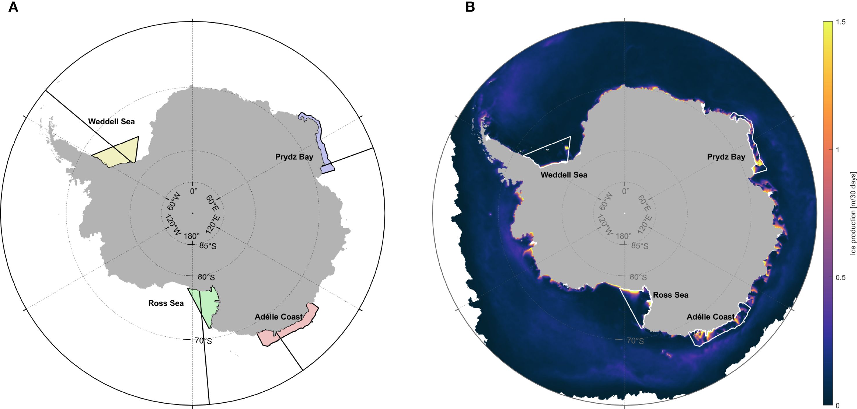
Figure 1. (A) Shaded polygons indicate the four main areas of dense water formation: Weddell Sea, Ross Sea, Prydz Bay, and Adélie Coast. Black lines show the meridional transects (310°E, 175°E, 70°E, 145°E) used to assess latitudinal variability in physical variables and surface heat fluxes. (B) Mean sea-ice production from March to October (2003-2010) highlighting coastal polynya hotpots, with the four main areas of dense water formation delimited in white line.

In these locations, shelf processes, coastal polynya dynamics, and brine rejection during sea-ice formation promote the generation of DSW that cascade down the continental slope and mix with warmer or fresher Southern Ocean waters, mostly CDW and Antarctic Surface Water, thereby contributing to this ventilation of the global abyss (Silvano et al., 2023). Specifically, in the ice-free coastal polynyas over the Antarctic continental shelf is where the High-Salinity Shelf Water (HSSW) is produced as a result of surface heat loss and salt input through brine rejection when sea ice forms. Freshwater fluxes from precipitation, ice-shelf melt, and sea-ice melt can counteract this salinification, modulating dense water formation and its variability (Pellichero et al., 2018). Then, HSSW undergoes additional cooling through mixing with basal meltwater beneath ice shelves, resulting in the formation of supercooled Ice Shelf Water (ISW). A portion of this ISW subsequently escapes the continental shelf and descends into the abyssal Southern Ocean. Both dense waters produced on the continental shelf (HSSW and ISW) are usually referred altogether as DSW (Silvano et al., 2023). Hence, the net heat loss from the ocean to the atmosphere is therefore a direct contributor to the generation of HSSW as well as in promoting upper-ocean destabilization and initiating convective overturning processes. In this sense, surface heat fluxes are more than just an energy exchange term: they encapsulate a key control on the transformation of water masses and the ventilating mechanisms of the deep ocean. These underlaying mechanisms have been studied extensively through both hydrographic campaigns and process-based analyses, such as in Meredith et al. (2000), which examined the source pathways of dense waters in the Weddell Gyre. Observational evidence of sustained AABW contraction over recent decades further supports the view that dense water formation is declining and hence weakening the deep overturning circulation around the Antarctica (Purkey and Johnson, 2012; Azaneu et al., 2013; Gunn et al., 2023; Zhou et al., 2023).

Moreover, an increasing number of modelling studies suggests that anthropogenic signals in the MOC may become evident first in the Southern Ocean. Lee et al. (2023), for instance, used a coupled ocean–sea ice diagnostic model to demonstrate that human-induced changes in overturning are now emerging from Antarctic latitudes. In parallel, modeling studies such as Heuzé (2020) and Lago and England (2019) have shown that ongoing changes in sea ice melt and freshwater input are likely to delay or weaken AABW formation in the coming decades. Similarly, Menezes et al. (2017) reported accelerated freshening and warming of AABW in the southern part of the Indian Ocean, suggesting a sustained decrease in bottom water density and a weakening of formation. These trends were linked in part to cryospheric perturbations, such as major iceberg calving events. High-resolution simulations by Jeong et al. (2023) further revealed that increased atmospheric CO₂ concentrations lead to surface freshening and substantially reduce DSW formation.

Building on this physical rationale, several studies have focused on quantifying surface heat fluxes and their role in controlling the thermohaline structure and ventilation of the deep ocean in polar regions. Fusco et al. (2009) and Budillon et al. (2000), for instance, analyzed the surface heat budget over the Ross Sea and the Terra Nova Bay polynya, revealing strong interannual variability in heat loss and its link to the production of HSSW. Newsom et al. (2016) highlights that a pronounced slowdown in the overturning circulation is primarily linked to reduced surface heat loss. In parallel, Holland et al. (2020) emphasized the importance of ocean circulation in regulating basal melting of Antarctic ice shelves and, by extension, the mass balance of the ice sheet. Complementary studies have also highlighted that water mass transformation in the Southern Ocean is strongly modulated not only by heat fluxes but also by freshwater and salt fluxes. For instance, Pellichero et al. (2018) and Abernathey et al. (2016) show that brine rejection and melt of sea ice dominate water mass transformations, specially influence upwelled CDW transformation, while Newsom et al. (2016) highlighted that the circulation is particularly sensitive to changes in surface transformation under atmospheric warming driven by rising CO₂ levels.

Despite the central importance of overturning circulation to the Earth system, direct observations of dense water formation remain sparse and geographically limited, particularly in the high-latitude Southern Ocean. This observational gap has led researchers to rely increasingly on indirect methods, including numerical models and reanalysis products. Among them, the ERA5 reanalysis output, developed by the European Centre for Medium-Range Weather Forecasts (ECMWF; Hersbach et al., 2020), offers a physically consistent, spatially continuous, and long-term estimate of atmospheric and surface fluxes. ERA5’s integration of satellite observations and improved model physics has enhanced its reliability in polar regions, making it a valuable resource for investigating dense water formation processes and their sensitivity to climate variability. By leveraging ERA5, this study aims to bridge existing observational gaps and provide a robust, large-scale assessment of surface heat fluxes across key AABW formation zones.

In this context, the present study aims to characterize spatial and interannual variability in surface heat fluxes across the main Antarctic dense water formation regions using ERA5 reanalysis. Specifically, we focus on identifying long-term trends and shifts in surface thermal forcing that modulate the ocean–atmosphere energy exchange. By tracking these fluxes and associated physical variables over time, we provide a clear and quantitative assessment of the ocean–atmosphere heat exchange processes that are critical to understanding the environmental conditions shaping bottom water formation.

2 Data and methods

2.1 Reanalysis output

This study utilizes output from the ERA5, which offers global estimates of atmospheric, land, and surface ocean variables, with a horizontal resolution of 0.25° × 0.25° (Hersbach et al., 2020). Specifically, we use the ERA5 single-level monthly mean output (reanalysis-era5-single-levels-monthly-means product) for the period from March to October, which corresponds to the austral autumn, winter, and early spring months, and is commonly considered to be the freezing period (Silvano et al., 2023). While the original ERA5 release provided output starting from 1979, the final version includes a back-extension covering the period 1940–1978. Based on the assessment by Bell et al. (2021), which indicates that ERA5 output achieves sufficient quality in the Antarctic region from the mid-1970s onward, this study only utilizes data from 1980 to 2024. This time range ensures both quality and sufficient temporal coverage to detect interannual variability and trends in the analyses.

To estimate the heat exchanges, we extract the main components of the surface energy balance: surface latent heat flux (L-HF), surface sensible heat flux (S-HF), surface net shortwave radiation flux (Net SWRF), and surface net longwave radiation flux (Net LWRF). All fluxes are expressed in W m⁻².

In addition to these surface fluxes, several physical variables are considered to provide context and assess the mechanisms influencing DSW formation. These include 2-metre air temperature (T_a), sea surface temperature (SST), 10-metre wind speed (zonal and meridional components, WS), sea ice cover (SIC), and incident solar radiation (ISR) for the same period and or the same period and spatiotemporal resolution.

2.2 Calculation of the ocean heat budget

The ocean heat budget (OHB) is assessed by considering the balance of incoming and outgoing heat fluxes at the ocean surface in contact with both the sea ice and the atmosphere. The surface heat flux Q (Equation 1) in a system involving interactions between the atmosphere, ice, and ocean can be decomposed as follows (Budillon et al., 2000):

$\begin{array}{ll}Q=Q_{SW}+Q_{LW}+Q_{SH}+Q_{LH}+Q_{COND}& (1)\end{array}$

where Q_SW is shortwave radiation, Q_LW is longwave radiation, Q_LH is latent heat flux, Q_SH is sensible heat flux, and Q_COND is the conductive heat flux (CF) through sea ice. The sign convention used throughout this manuscript is that fluxes are considered positive when the ocean gains heat.

The individual terms are computed as follows (ECMWF, 2024) (Equations 2–6). Short-wave radiation is given by:

$\begin{array}{ll}{Q}_{SW}=(1-\alpha )F_0& (2)\end{array}$

where α is the surface albedo and F₀ (W m⁻²) is the incoming solar radiation. Long-wave radiation follows the Stefan-Boltzmann law:

$\begin{array}{ll}{Q}_{LW}=\in (R_T-\sigma T_{sk}^4)& (3)\end{array}$

where ∈ is the surface emissivity, R_T is the downward longwave radiation from the atmosphere (W m⁻²), σ is the Stefan-Boltzmann constant (5.67× 10⁻⁸ W m⁻² K⁻⁴), and T_sk is skin temperature (K), equivalent to the SST over the ocean. Sensible heat flux is calculated as:

$\begin{array}{ll}{Q}_{SH}={\rho }_a{C}_H{c}_p\left|U\right|(T_a-T_{sk})& (4)\end{array}$

where ρ_a is the density of the air above the ocean (kg m⁻³), C_H is the sensible heat transfer coefficient, c_p is the specific heat (J kg⁻¹ K⁻¹), U is wind speed (m s⁻¹), T_a is air temperature (K). Latent heat flux is given by:

$\begin{array}{ll}{Q}_{LH}={\rho }_a{C}_Q\left|U\right|(q_a-q_{sat}(T_{sk}))L_v& (5)\end{array}$

where C_Q is the moisture transfer coefficient, q_a is specific humidity, and q_sat(T_sk) is saturation humidity at T_sk and L_v is the evaporation latent heat (J kg⁻¹). CF through ice is expressed as indicated in Semtner (1976) and Budillon et al. (2000):

$\begin{array}{ll}{Q}_{COND}=\frac{K_i}{d_e}(T_{sfc}-T_b)& (6)\end{array}$

where K_i =2.04 Wm⁻¹K⁻¹ is the thermal conductivity of ice, d_e is the effective ice layer thickness, T_sfc is the ice surface temperature, and T_b is the basal ice temperature, approximated as the freezing point of seawater (-1.8 °C or 271.35K). The effective ice thickness d_e is determined dynamically from ERA5 variables, selecting the deepest available ice temperature layer to assign T_b and the corresponding depth. Each layer depth is defined as the mean of each layer range: Layer 1 (0–7 cm, mean 3.5 cm), Layer 2 (7–28 cm, mean 17 cm), Layer 3 (28–100 cm, mean 64 cm), and Layer 4 (100–150 cm, mean 125 cm). If the temperature at the deepest layer is available, it is used; otherwise, the deepest available valid layer is chosen.

2.3 Spatial Integration of the heat budget in dense water formation regions

To analyze the interannual variability of the ocean heat budget, the final balance is integrated over the four dense water formation regions, defined by Schmidt et al. (2023): Weddell Sea, Ross Sea, Adélie Coast and Prydz Bay. These regions are characterized by strong surface water mass transformation and enhanced sea-ice production, providing a physically consistent framework for assessing DSW formation. Since the ERA5 outputs are provided in degrees, converting them into physical distances requires accounting for the Earth’s sphericity. This is particularly important in polar regions, where the convergence of meridians causes notable variations in grid cell size.

In a spherical projection, the area of each grid cell is proportional to the cosine of the latitude. The differential area element for a latitude-longitude grid in geographic coordinates is given (Equation 7):

$\begin{array}{ll}dA=R^2 \text{cos}(\varphi )d\varphi d\lambda & (7)\end{array}$

where R is the Earth’s radius (approximately 6371km), ϕ is latitude, λ is longitude, and dϕ and dλ are the latitude and longitude increments of the grid, which are converted into radians. This correction ensures that the integral calculations accurately represent physical processes in dense water formation regions and provide a robust basis for analyzing interannual variability.

2.4 Calculation of flux contributions to ocean heat budget

To quantify the relative importance of each surface heat flux component, we compute for each region and year both:

2.4.1 Absolute contribution:

$$P_i^{\text{abs}}(t)=\frac{|Q_i(t)|}{{\sum }_{j=1}^5|Q_j(t)|}\times 100\%,$$

where Q_i are the annual, March–October averaged integrated fluxes, and the subscripts i and j denote each of the five flux components: L-HF, S-HF, Net SWRF, Net LWRF, and CF.

2.4.2 Signed contribution

$$P_i^{\text{sign}}(t)=\frac{Q_i(t)}{{\sum }_{j=1}^5{Q}_j(t)}\times 100\%,$$

which preserves the sign of each term. The percentages sum to 100% only if the total budget is non-zero.

These metrics allow us to distinguish between the overall strength (magnitude) and the net effect (warming or cooling) of each component’s contribution to the OHB.

2.5 Sea ice production data for coastal polynyas

To confirm whether the study areas selected by Schmidt et al. (2023) coincide with the key productive coastal polynyas where the surface dense water transformation occurs, we incorporated a satellite-based dataset of sea ice production (SIP) specifically developed for the Southern Ocean. Monthly SIP fields were obtained from the AMSR-E Polar Research Group archive at Hokkaido University. The dataset provides daily estimates of sea ice production on a polar stereographic grid with a spatial resolution of 6.25 km, subsequently aggregated into monthly means.

The product combines AMSR-E passive microwave observations with ERA5 atmospheric reanalysis at 0.25° × 0.25° resolution. The estimation of ice production is based on a thin ice thickness algorithm with ice-type discrimination (active frazil vs. thin solid ice), initially developed by Nakata et al. (2019), and further applied to produce spatial maps of active frazil ice formation and sea ice production in Antarctic coastal polynyas (Nakata et al., 2021).

In this study, we used the monthly climatology of sea ice production during March–October (2003–2010) to highlight the main coastal polynya hotspots in the Antarctic continent surroundings (Figure 1B).

3 Results

This section presents the results beginning with a large-scale characterization of physical variables and surface fluxes across the Southern Ocean south of 60°S. This is followed by a latitudinal analysis along four selected meridional sections, and concludes with a temporal assessment of conditions in the four key continental shelf regions where dense water is formed. Within this final part, particular attention is given to the evolving contributions of individual surface heat flux components to the OHB, highlighting shifts in their relative importance over time.

3.1 Climatological distributions

The large-scale distribution of physical variables and fluxes over Antarctica and Southern Ocean surroundings are presented in Figures 2 and 3, averaged from March to October during the period 1980 to 2024. Near the Antarctic coastline, SST typically approach the freezing point, and gradually increase northward, often reaching 1–3 °C (or slightly higher) in open-ocean regions (Figure 2A). Over the continental interior, extremely cold T_a conditions prevail, with mean values often quite below -30 °C (not shown), rising to above -20 °C near the coast or over open water (Figure 2B). Regarding the SIC, coastal waters and high-latitude regions typically display near 100% coverage (values close to 1.0), creating a pronounced gradient of sea ice extent that decreases toward lower latitudes. In these regions, SIC may drop below 0.5 in summer although persistent sea ice, such as landfast ice, plays a significant role in maintaining higher concentrations in coastal areas, even during this period (areas with sea ice concentration ≥15% are considered ice-covered; otherwise, are considered ice-free; Figure 2C). Average wind intensities can vary considerably from gentle breezes (under 5 m s ⁻¹) to stronger flows above 10 m s ⁻¹, especially near the coastal margins and over the open ocean where atmospheric systems drive more vigorous circulation (Figure 2D). Finally, ISR values are generally lower over the pole and near the continent, reflecting the high latitude and persistent cloud/ice cover, but they can reach 1.5-2×10⁷ W m⁻² or more in areas of lower latitude and clearer skies.

Figure 2

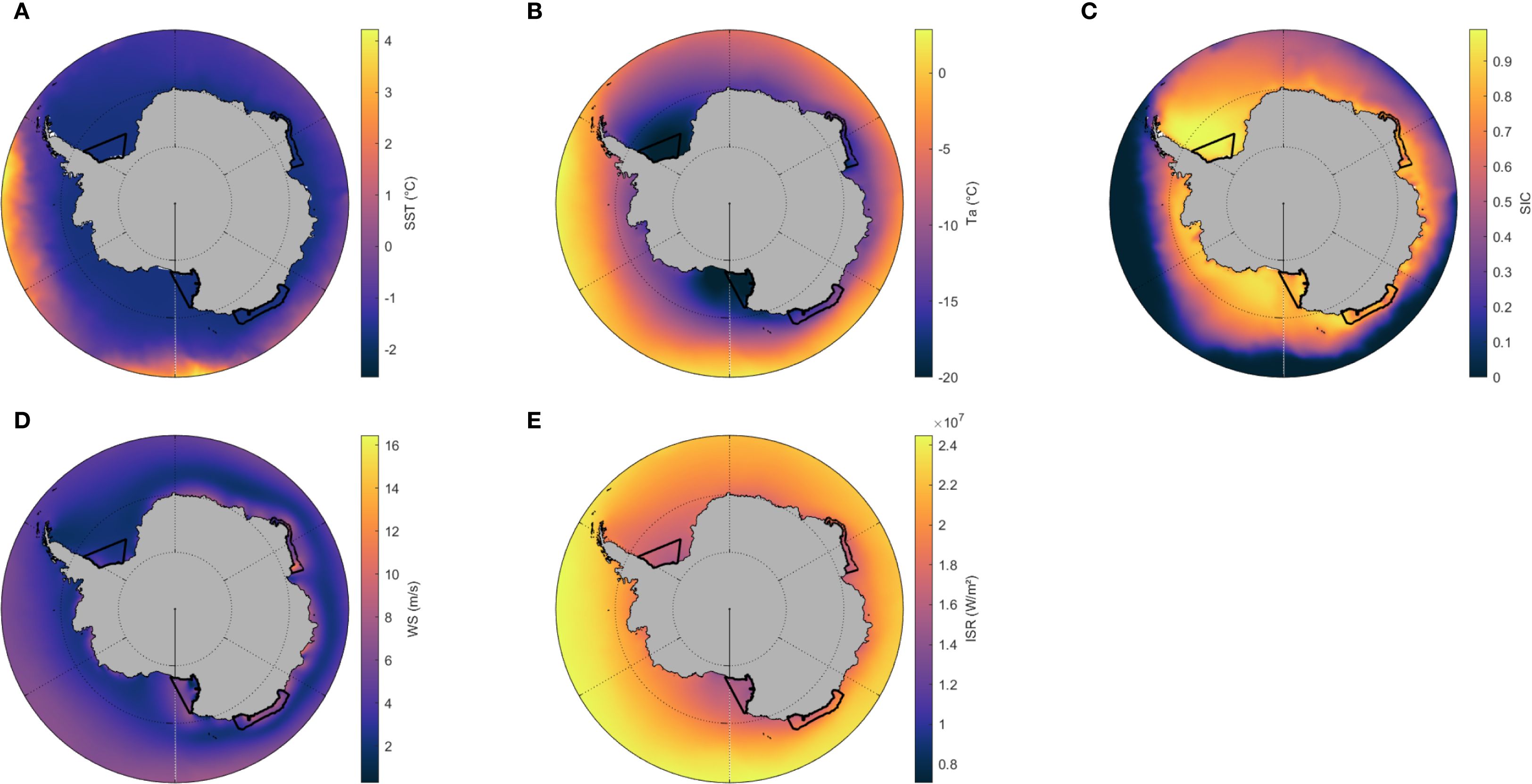
Figure 2. Mean state of key physical variables around Antarctica and over the Southern Ocean (1980–2024, March–October). (A–E) show sea surface temperature (SST), near-surface air temperature (T_a), sea-ice concentration (SIC), wind speed (WS), and incident solar radiation (ISR). The outlines of the main Dense Shelf Water or DSW formation regions (see Figure 1) are overlaid for reference.

Figure 3

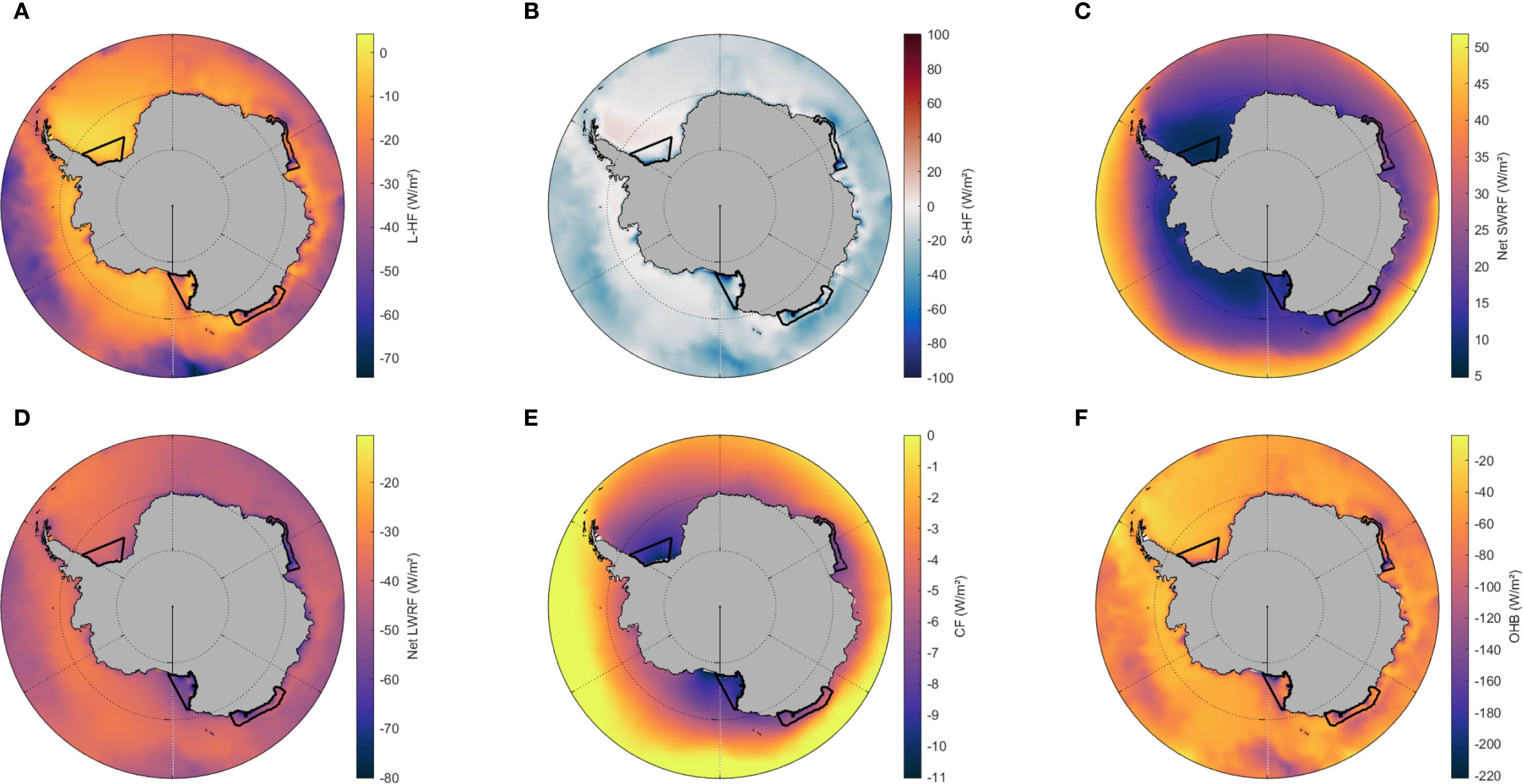
Figure 3. Mean state of surface heat flux components over Antarctica and the Southern Ocean (1980–2024, March–October). (A–F) show latent heat flux (L-HF), sensible heat flux (S-HF), net shortwave radiation flux (Net SWRF), net longwave radiation flux (Net LWRF), conductive flux (CF), and the ocean heat budget (OHB). The outlines of the main Dense Water formation regions (see Figure 1) are overlaid for reference.

Analyzing different components of the surface heat fluxes, L-HF typically takes negative values from about -20 W m⁻² to -5 W m⁻² across different regions, with strongest losses over open ocean where evaporation is highest (Figure 3A). The mean evaporation pattern (Supplementary Figure S1) shows maxima over the open Southern Ocean, particularly in ice-free regions north of 65°S, spatially coinciding with the strongest latent heat losses. This spatial agreement supports the link between L-HF and evaporation; however, other factors such as wind speed, near-surface humidity gradients, and sea ice conditions also modulate the magnitude of these losses. S-HF measures the direct transfer of heat between the surface and the atmosphere, commonly spanning from around -30 W m⁻² to +30 W m⁻², depending on air–sea (or air–sea-ice) temperature differences (Figure 3B). Net SWRF is always positive and can range from some 20 W m⁻² in areas with high albedo and reflection (especially over ice) up to 40–50 W m⁻² in regions with stronger incoming solar radiation and lower reflectivity (Figure 3C). The ocean typically loses heat via longwave emission, so the Net LWRF always takes negative values which are typically around -20/-30 W m⁻², taking values of -60 W m⁻² or below at some locations close to the continent (Figure 3D). CF generally constitutes a smaller component except where strong temperature gradients exist in ice or shallow ocean layers (Figure 3E); values are always negative in the range from 0 to -11 W m⁻². These fluxes combine in the OHB, which remains negative across the Southern Ocean, reflecting net surface heat losses to the atmosphere. The strongest values (up to –220 W m⁻²) occur near the Antarctic continent, particularly within the four main dense water formation zones (Figure 3F).

Within this climatological characterization of the surface physical variables and fluxes, the standard deviation (hereafter std for simplicity) is also assessed (Supplementary Figure S2). The interannual variability of SST is lowest along the South Atlantic and eastern Pacific sectors, near the mean position of the sea-ice edge reflecting lower year-to-year fluctuations in the ice–open-ocean boundary. The std of T_a displays a nearly opposite pattern, with maximum variability over the Antarctica’s coastal margins, especially in Adélie Coast, Wilkes Land, and the Antarctic Peninsula. These regions are more exposed to interannual atmospheric fluctuations, including warm-air intrusions and changes in surface albedo due to snow and ice conditions, while over the open ocean, air temperature variability is significantly lower. SIC variability peaks in the marginal ice zone, particularly in the Bellingshausen and Amundsen Seas, and north of the Weddell Sea, where the ice edge is most mobile, even with small latitudinal shifts in the ice margin, and it is minimal at locations closer to the continent, particularly at Weddell Sea, and in the open ocean. Wind speed shows moderate variability with a distinct maximum near 60°S in the Pacific and Indian sectors, aligned with the core of the westerly wind belt. The std of ISR is highest over the open Southern Ocean north of the sea-ice edge, spanning the Pacific, Atlantic, and Indian sectors. These regions are known to experience strong interannual fluctuations in cloud cover, solar zenith angle, and seasonal atmospheric dynamics, which modulate incoming solar radiation. In contrast, coastal Antarctic regions and the interior of the ice-covered seas display very low variability due to persistent sea-ice cover and reduced solar input during the March–October period.

With respect to fluxes, L-HF variability is highest along specific Antarctic coastal margins, particularly in the eastern Weddell Sea and the Adélie–Wilkes Land coast (Supplementary Figure S3). In contrast, most of the Amundsen and Bellingshausen Seas, along with the interior of the Weddell and Ross Seas, show low variability, consistent with persistent ice cover that dampens surface exchange processes. S-HF displays a pattern similar to L-HF, though generally with lower amplitude with high variability again concentrated near polynya-prone coastal regions, where strong ocean–atmosphere thermal gradients vary significantly interannually. Ice-covered regions show low std of S-HF, reflecting the insulating effect of the ice. The standard deviation of Net SWRF is largest in partially ice-covered coastal zones near the western Antarctic Peninsula, along the Adélie Land coast, and in the vicinity of Prydz Bay, due to variability in surface albedo and cloud cover. Areas with persistent sea ice or cloud cover have low variability. These patterns suggest that even modest shifts in sea-ice concentration or atmospheric transparency can substantially alter the surface ocean’s ability to absorb incoming solar radiation, primarily through changes in surface albedo. Net LWRF shows low and uniform interannual variability, with slightly elevated std values over open-ocean sectors and in some coastal regions of East Antarctica. This relative stability, more pronounced compared to other flux components, reflects the consistent longwave radiative cooling of the surface, weakly modulated by changes in surface temperature and cloud-induced variations in downward longwave radiation. CF variability is highest within ice-covered continental shelves of the Weddell Sea, Ross Sea, Prydz Bay, and the Adélie Coast, linked to interannual changes in sea-ice thickness, snow layering, and vertical temperature gradients, which directly affect conductive heat transfer. In contrast, it is minimal in the open ocean north of 65°S and over the Antarctic continent, reflecting the absence of sea ice in the former and minimal surface energy exchange in the latter. Contrary to other flux components, CF variability is not concentrated at the ice edge, but rather within the ice-covered regions, emphasizing the dynamic nature of conductive processes over the Antarctic ice shelves.

The interannual std of OHB displays a spatially heterogeneous structure. Elevated variability is observed in the open Southern Ocean north of 70°S, particularly in the Pacific and Indian sectors, and over the continental shelves mainly of Prydz Bay, Adélie Coast, and the eastern Ross Sea, where surface fluxes are strongly modulated by seasonal polynyas. The Weddell Sea area stands out as one of the most stable in terms of OHB interannual fluctuations, likely due to persistent multiyear ice cover and limited surface exchange. Other low-variability areas of OHB include the interior of the Amundsen and Bellingshausen Seas. Pockets of elevated variability also appear in the circumpolar South Atlantic and Scotia Sea, possibly linked to shifting atmospheric patterns or Antarctic Circumpolar Current frontal dynamics (Thompson and Youngs, 2013; Gurjão et al., 2025). Overall, OHB variability reflects the interplay between turbulent and radiative flux components, constrained by the presence or absence of sea ice, with the strongest year-to-year changes occurring near dynamically active coastal zones and marginal sea-ice areas.

3.2 Long-term trends

The dataset spans 45 years at monthly resolution, resulting in a time series of 540 monthly values per grid cell. Linear trends are computed for each variable at every grid point, revealing spatial patterns of long-term changes in the Antarctic system.

We first assessed the robustness of the trends in order to identify which regions exhibit statistically significant long-term changes. Supplementary Figures S4 and S5 present the spatial distribution of p-values corresponding to the linear trends computed for each surface variable and flux component during the March–October period over 1980–2024. The strongest and most widespread significance is observed in SST and T_a (Supplementary Figures S4A, B) over the northern sector of the Southern Ocean. Additional hotspots of significance are found on the continental shelf, mainly between 90°E and 175°E in the western Pacific Ocean sector—Adélie and Wilkes Lands— as well as in the southeastern Weddell Sea, the tip of Antarctic Peninsula and the Bellingshausen Sea, where p-values frequently fall below 0.01. Wind speed is generally weak and spatially heterogeneous, exhibiting limited statistical significance, whereas ISR show localized but meaningful areas of significance, suggesting regionally coherent atmospheric shifts (Supplementary Figures S4C, D). In contrast, SIC (Supplementary Figure S4E) exhibits broader areas of low p-values, particularly over the continental shelf and along the ice edge, consistent with seasonal sea ice changes and documented long-term changes in sea ice extent.

Among the heat fluxes, L-HF and S-HF (Supplementary Figures S5A, B) present scattered yet relevant areas of significance, mostly around coastal polynyas and marginal ice zones, indicating that interannual variability in air–sea turbulent exchange is not purely random. Radiative fluxes—Net SWRF and Net LWRF (Supplementary Figures S5C, D)—display more spatially coherent zones of significance, especially for Net SWRF, likely reflecting changes in cloud cover, sea-ice albedo, and surface radiative balance. CF (Supplementary Figure S5E) shows significant trends predominantly along the coastal shelf and sea-ice transition zone, closely following T_a significance pattern and reinforcing its sensitivity to ice thickness and temperature gradients. Finally, the OHB trend (Supplementary Figure S5F) is statistically significant across several key areas, including the Ross Sea, Weddell Sea, and Adélie Coast, supporting its use as an integrated indicator of long-term changes in surface heat exchange in dense water formation regions.

After establishing the robustness of the signals, we now describe the spatial patterns of the long-term trends. Figure 4 displays linear trends in five key physical variables around Antarctica. SST and T_a trends (Figures 4A, B) reflect warming or cooling of up to 0.2 °C/decade. The strongest SST cooling trends are observed in the eastern Pacific sector, north of approximately 65°S, while warming dominates southward, particularly pronounced in the western Antarctic Peninsula, the Bellingshausen Sea and Amundsen Sea. The Indian Ocean sector also shows predominantly a warming tendency, whereas in the Weddell Sea, trends are weaker and more spatially variable, often close to zero, remaining stable. The T_a trends present a more alternating spatial pattern: warming trends north of the Weddell Sea, reaching maximum values of 0.2 °C/decade, and negative trends in the eastern South Atlantic sector, mainly localized close to Queen Maud Land coast (between 0 - 45°E). Further east, positive trends re-emerge in the Indian sector up to around 80°E, after which a broad region of negative trends dominates until approximately 180°E. Beyond the Ross Sea, trends become positive again, before turning negative in the Amundsen Sea, and finally shifting back to a strong warming signal over the Bellingshausen Sea and the Antarctic Peninsula.

Figure 4

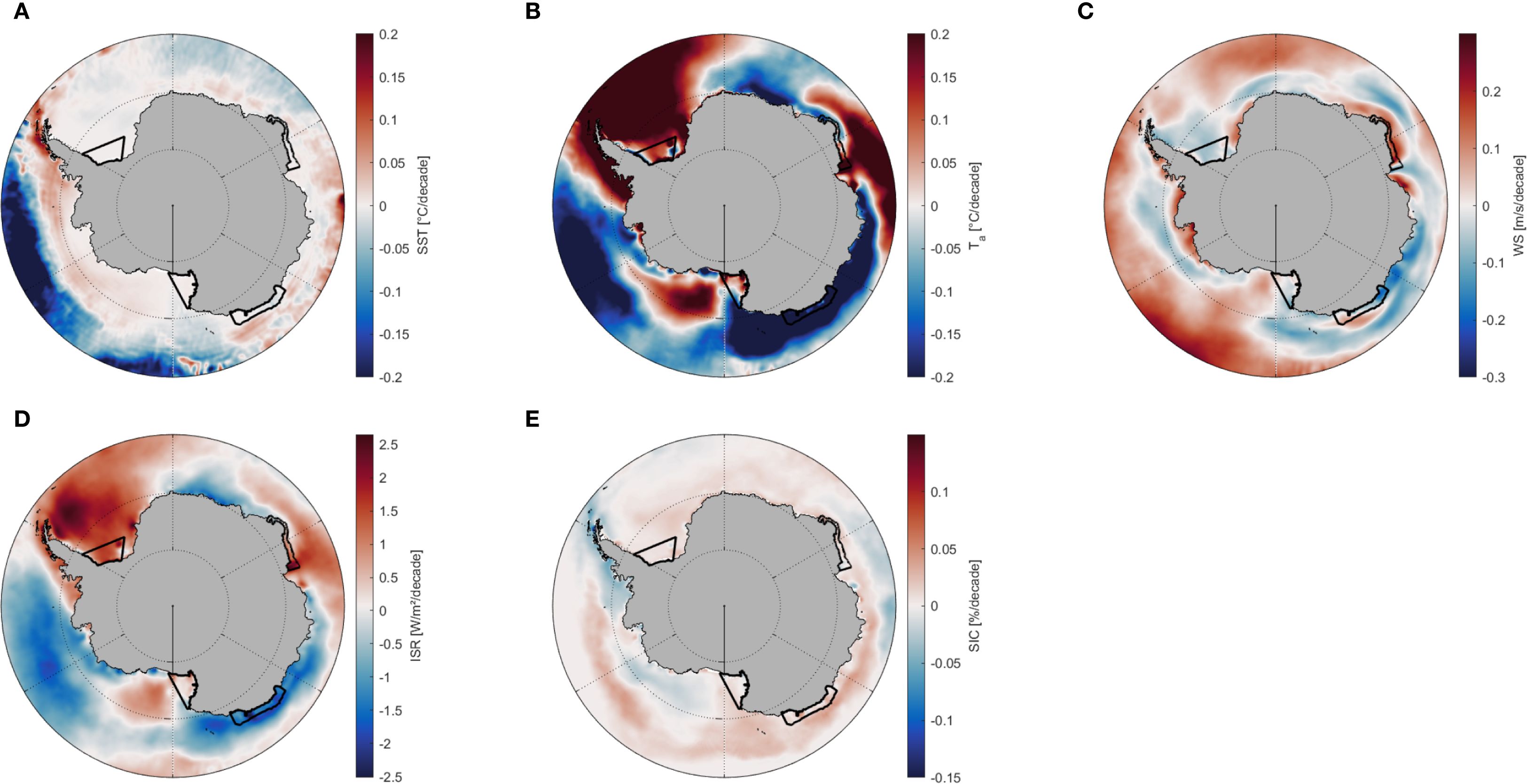
Figure 4. Linear trends (1980–2024, March–October) in key physical variables around Antarctica. (A–E) show direct trends in sea surface temperature (SST, °C/decade), near-surface air temperature (T_a, °C/decade), wind speed (WS, m/s/decade), incident solar radiation (ISR, W/m²/decade), and sea-ice concentration (SIC, %/decade). Negative (blue) and positive (red) values indicate decreasing or increasing trends, respectively. The outlines of the main Dense Shelf Water or DSW formation regions (see Figure 1) are overlaid for reference.

The wind speed panel shows predominantly an intensification of the Southern Ocean westerlies at latitudes north of approximately 65°S, transitioning to weaker winds farther south, with small positive anomalies in localized coastal regions. At the fourth panel, ISR displays very weak trends, generally between -1 and +1 W m⁻² per decade, with positive trends in the Weddell Sea, western side of the Antarctic Peninsula, Prydz Bay and in localized regions of the Ross Sea. In Figure 4E, SIC trends range from -0.15 to +0.05% per decade, remaining the sea-ice concentration stable or with a slight increase across most of the Southern Ocean. However, negative trends are evident in western Antarctic Peninsula, in the Amundsen Sea, and in the Prydz Bay—precisely the areas where the strongest warming trends in T_a are also observed.

In Figure 5, each panel represents a different surface heat flux component. Interpreting surface heat flux trends require consideration of both the trend maps and the mean state shown in Figure 3. A positive trend in a predominantly positive variable indicates intensification of the flux, whereas a positive trend in a predominantly negative variable implies a weakening of that flux—meaning the values are becoming less negative. Once said that, although the color bar is set in all cases from -100 to +100 W m⁻²/decade, for consistency and better comparison between them, many regions exhibit moderate magnitudes, corresponding roughly to -10 to +10 W m⁻²/decade in real terms.

Figure 5

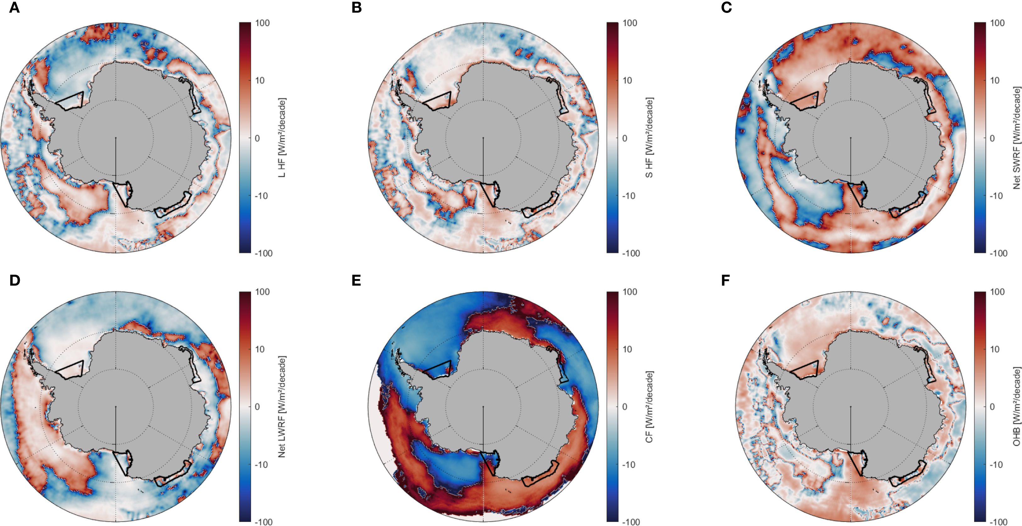
Figure 5. Linear trends (1980–2024, March–October) in surface heat flux components around Antarctica. (A–F) show latent heat flux (L-HF), sensible heat flux (S-HF), net shortwave radiation flux (Net SWRF), net longwave radiation flux (Net LWRF), conductive flux (CF), and the ocean heat budget (OHB). Trends are represented on a signed logarithmic scale ranging from approximately –100 to +100. Negative (blue) and positive (red) values indicate whether each component has decreased or increased over time. The outlines of the main Dense Shelf Water or DSW formation regions (see Figure 1) are overlaid for reference.

Both L-HF and S-HF show a patchwork of positive (reds) and negative (blues) trends, suggesting that evaporation/sublimation and turbulent heat exchanges are intensifying in some areas while diminishing in others heterogeneously. Remarkable positive trends are observed along the coast near the Antarctic Peninsula, Bellingshausen Sea, and Amundsen Sea, as well as in the offshore Indian and Australian sectors, whereas negative trends or stationary responses are evident in the Weddell Sea, Ross Sea, and along the nearshore of the Indian sector. These trends somewhat mirror the distribution already described for the T_a, indicating that where the T_a is rising, S-HF is also increasing—implying that the positive values are becoming larger while the negative values are becoming less pronounced except for the Weddell Sea.

Net SWRF shows a broad pattern of positive trends across most of the Antarctic coastline, particularly in the Weddell Sea, Ross Sea, and Adélie Coast, suggesting an increase in incoming shortwave energy over these regions during the March–October period. Negative trends, though less spatially extensive, are observed mainly in the Amundsen and Bellingshausen Seas, the eastern Weddell, and some localized offshore areas in the Indian sector. In contrast, Net LWRF displays strongly positive trends across the Amundsen and Bellingshausen Seas, the western Weddell, and the Indian and Australian sectors, pointing to an enhanced greenhouse effect and increased longwave energy loss. Negative trends are restricted to more localized regions, including parts of the Ross Sea, Prydz Bay, and the eastern coast of Queen Maud Land. The CF presents a spatial pattern broadly anti-correlated with T_a trends, showing decreasing values where surface air temperature increases, and vice versa. This inverse relationship is especially evident in West Antarctica, Wilkes Land, and along parts of the Weddell Sea margin, consistent with the sensitivity of CF to vertical temperature gradients across the snow and ice layers.

Finally, the OHB panel integrates all surface heat flux components, revealing where the net oceanic heat gain (red) or loss (blue) is intensifying or weakening (Figure 5F). The spatial pattern is complex but not entirely patchy, with coherent positive trends emerging over the Weddell Sea, Adélie Coast, and parts of the Ross Sea shelf, indicating a reduction in net oceanic heat loss in regions traditionally associated with strong surface cooling. In contrast, negative OHB trends dominate the Wilkes Land margin and parts of the Amundsen and Bellingshausen Seas, suggesting an intensification of oceanic heat loss in these areas. The positive OHB trend in the Weddell Sea—where the mean heat budget remains negative—indicates a weakening of net cooling, consistent with the interpretation for the Ross and Amundsen Seas, where positive trends in OHB coincide with predominantly negative long-term values. These spatial variations in OHB trends may reflect shifts in the balance among turbulent, radiative, and conductive processes, modulated by changes in sea ice and atmospheric forcing.

3.3 Latitudinal variability at selected sections

We now focus on the four key regions of interest to analyse in greater detail how surface heat fluxes, physical variables and their long trends influence dense water formation, using targeted meridional transects to capture latitudinal gradients from the open ocean to the Antarctic continental margin. The analysis is based on the latitudinal variability of these physical variables averaged over the period 1980–2024 for the March-October months (Figure 6). For each region, we selected the meridional transect from 60°S extending furthest south to capture the longest possible record in proximity to the continent (see the position of the latitudinal transects in Figure 1A). T_a consistently exhibits minimum values near the continent, approximately –25 °C in the Weddell and Ross Seas, increasing progressively toward the north, reflecting the strong continental cooling influence of Antarctica. SST remains predominantly at or near the freezing point of seawater (–1.8 °C), likely due to the extensive sea-ice cover in winter, rising to positive values only in the northernmost sections beyond roughly 62–63°S in both the Ross Sea and Adélie Coast regions.

Figure 6

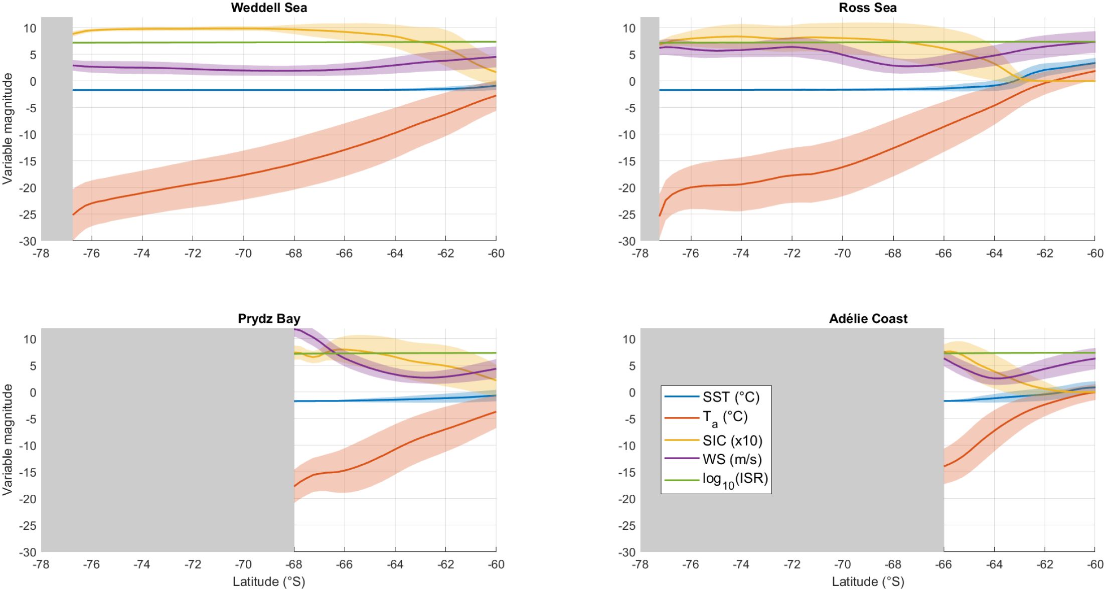
Figure 6. Latitudinal variability of selected physical variables along the four DSW formation regions sections around Antarctica (Weddell Sea, Ross Sea, Prydz Bay, and Adélie Coast). The locations of these sections correspond to the latitudinal transects indicated in Figure 1. Variables displayed include sea surface temperature (°C), air temperature (°C), sea-ice concentration (scaled by a factor of 10 for clarity), wind speed (m/s), and ISR (log10). Shaded areas represent latitudes with no available data due to the presence of land or ice shelf. Solid lines represent the climatological mean of each variable, while the surrounding shaded areas indicate the interannual standard deviation.

Wind speed generally remains moderate, averaging around 2–3 m s⁻¹, and intensifies further north where westerlies dominate as well as near the continent, particularly evident in Prydz Bay and the Adélie Coast, surpassing 10 m s⁻¹ in Prydz Bay. This intensification near the continent reflects persistent katabatic winds descending from the Antarctic Ice Sheet, particularly during winter months (Dong et al., 2020; Caton Harrison et al., 2024). These winds shape local weather patterns and are the primary drivers of coastal polynya formation, as they remove and export the newly formed sea ice and sustain open-water areas that facilitate coastal ocean–atmosphere exchanges (Zhang et al., 2024; Golledge et al., 2025).

SIC demonstrates distinct regional differences: it is minimal north of approximately 62–63°S in the Ross Sea and Adélie Coast, increasing rapidly southward with values surpassing 50% at the Ross Sea and smoothly at Adélie Coast, and shows low interannual variability in the extent of the sea ice coverage in the Weddell Sea. In the Weddell Sea, sea-ice concentration reaches nearly complete coverage (∼100%) across a large portion of the analyzed domain– from 68 to 75°S–, decreasing slightly near coastal areas, likely due to the presence of the Weddell Polynya. A similar pattern is observed in Prydz Bay, where sea-ice coverage also increases markedly toward the continent. ISR exhibits a latitudinal gradient, increasing northward from 1.5–1.8×10⁷ to 2.2–2.4×10⁷ W m⁻². This distribution underscores the strong dependence of solar energy input on latitude, with implications for melting dynamics and the seasonal evolution of sea ice.

The latitudinal distribution of surface heat fluxes is presented in Figure 7, following the same four meridional sections. Recall that negative surface flux values denote heat release from the ocean surface to the atmosphere. Net SWRF remains consistently positive in all four regions across the entire latitudinal span considered. This radiative input increases gradually toward lower latitudes (northward), becoming especially notable north of approximately 64°S. The remaining components are predominantly negative, representing heat loss from the ocean. For instance, CF through sea ice remains negative and mostly negligible across all sections, indicating a limited direct contribution to the net ocean–atmosphere heat exchange.

Figure 7

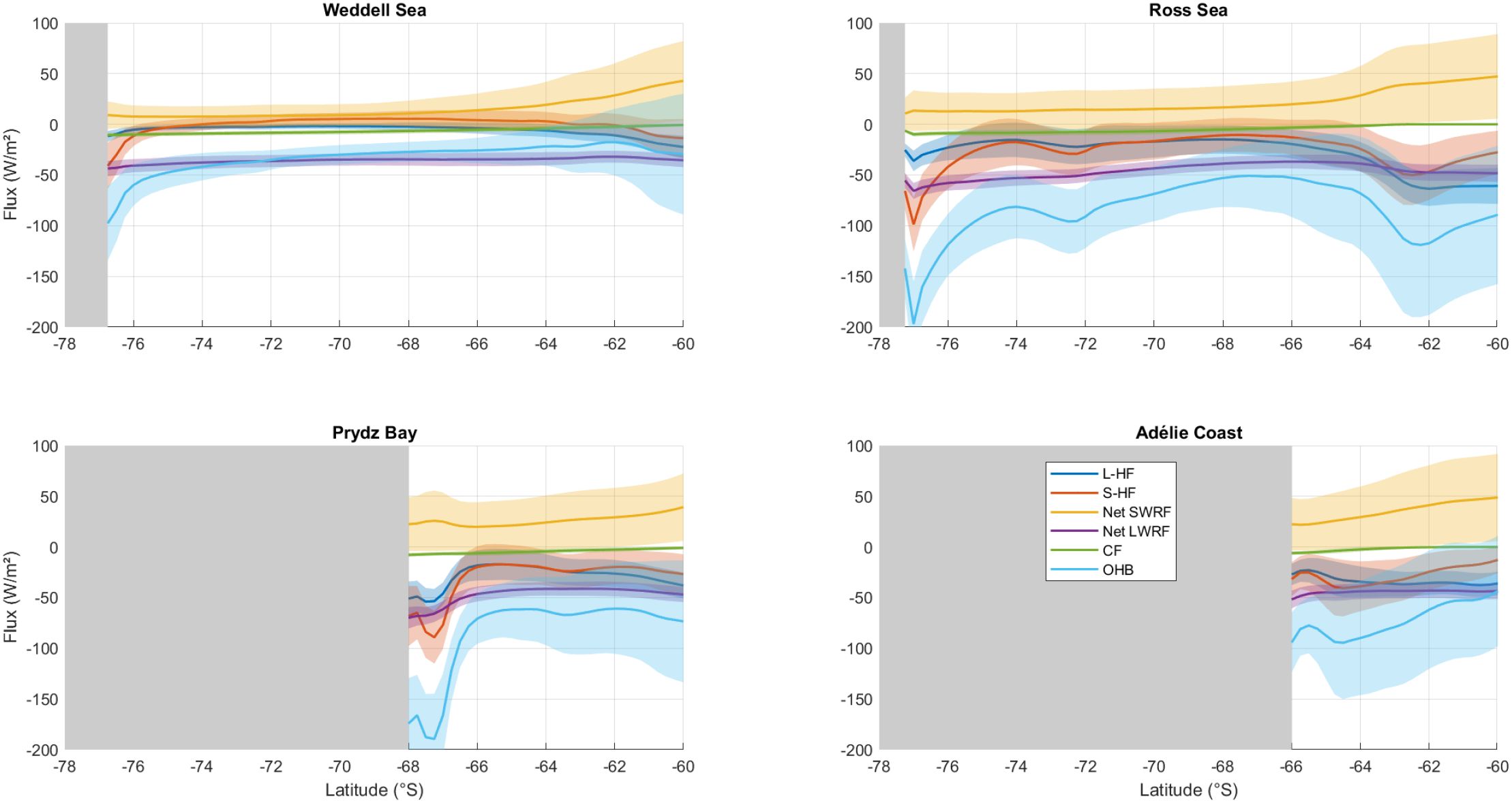
Figure 7. Latitudinal profiles of surface heat flux components (latent, sensible, shortwave net, longwave net, and conductive fluxes) and total ocean heat budget along four meridional sections (Weddell Sea, Ross Sea, Prydz Bay, and Adélie Coast). Negative fluxes indicate oceanic heat loss to the atmosphere, highlighting regions significant for Dense Shelf Water or DSW formation. The shaded grey areas represent latitudes without available data. Solid lines represent the climatological mean of each variable, while the surrounding shaded areas indicate the interannual standard deviation.

Net LWRF consistently emerges as the dominant contributor to oceanic heat loss, maintaining strong negative values across all sections, highlighting radiative cooling of the ocean surface as a major control on regional heat budgets. Generally, L-HF is more significant than S-HF in offshore areas. However, S-HF undergoes a sharp intensification – reaching the lowest values, i.e., maximum heat loss, except for the Adélie Coast – near the Antarctic coastline, emphasizing the role of atmospheric convection and strong thermal gradients between cold continental air and relatively warmer ocean surfaces—particularly in regions where dense water formation is most active.

Regional differences highlight the Ross Sea and Prydz Bay as areas of exceptionally intense oceanic heat loss, with OHB exceeding –180 W m⁻² near the Antarctic coast. In contrast, OHB is more moderate in the Weddell Sea and Adélie Coast (∼–100 W m⁻² maximum). These values reflect the dominance of strong surface cooling over the continental shelf, consistent with the presence of coastal polynyas, persistent katabatic winds, and efficient turbulent and conductive heat extraction—key conditions for dense water formation. In contrast, OHB in the Weddell Sea and Adélie Coast is comparatively moderate, reaching around –100 W m⁻² at most, with flatter latitudinal profiles and lower spatial gradients. This suggests that while these regions also contribute to dense water formation, the net surface cooling is less extreme, possibly due to thicker and more persistent sea-ice cover, which insulates the ocean from atmospheric forcing. The latitudinal structure of OHB also differs: in Ross Sea and Prydz Bay, OHB exhibits a sharp increase toward the coast, whereas in Weddell Sea and Adélie Coast it evolves more gradually, hinting at differing balances between radiative, turbulent, and conductive fluxes across sectors.

All four sections exhibit a consistent pattern of enhanced OHB, in magnitude, adjacent to the Antarctic continent, strongly supporting the formation of colder and saltier dense waters that contribute to AABW formation. Specifically, L-HF and S-HF become increasingly negative toward the coast, eventually surpassing the magnitude of Net LWRF in the Ross Sea and slightly at Prydz Bay.

3.4 Trends at selected locations

In this subsection, we focus the analysis of surface heat fluxes on the dense water formation areas. These polygons capture regions of intense surface water mass transformation, consistent with the location of coastal polynyas and associated brine rejection processes (Schmidt et al., 2023). The strength of coastal easterlies modulates sea-ice import and polynya extent, and their variability is a dynamic driver of the interannual variability observed within these regions. Hence, Figure 8 shows annual time series (1980–2024) of several key physical variables, spatially averaged over the four regions and from March to October. ISR remains remarkably constant across all four regions throughout the analyzed period, exhibiting minimal interannual variability. This suggests that recent changes in regional heat fluxes or ocean–atmosphere interactions cannot be attributed directly to variations in solar forcing. Similarly, SST remains consistently stable at around –1.8 °C in all regions, reflecting near-freezing ocean conditions and showing no apparent response to the global warming trends.

Figure 8

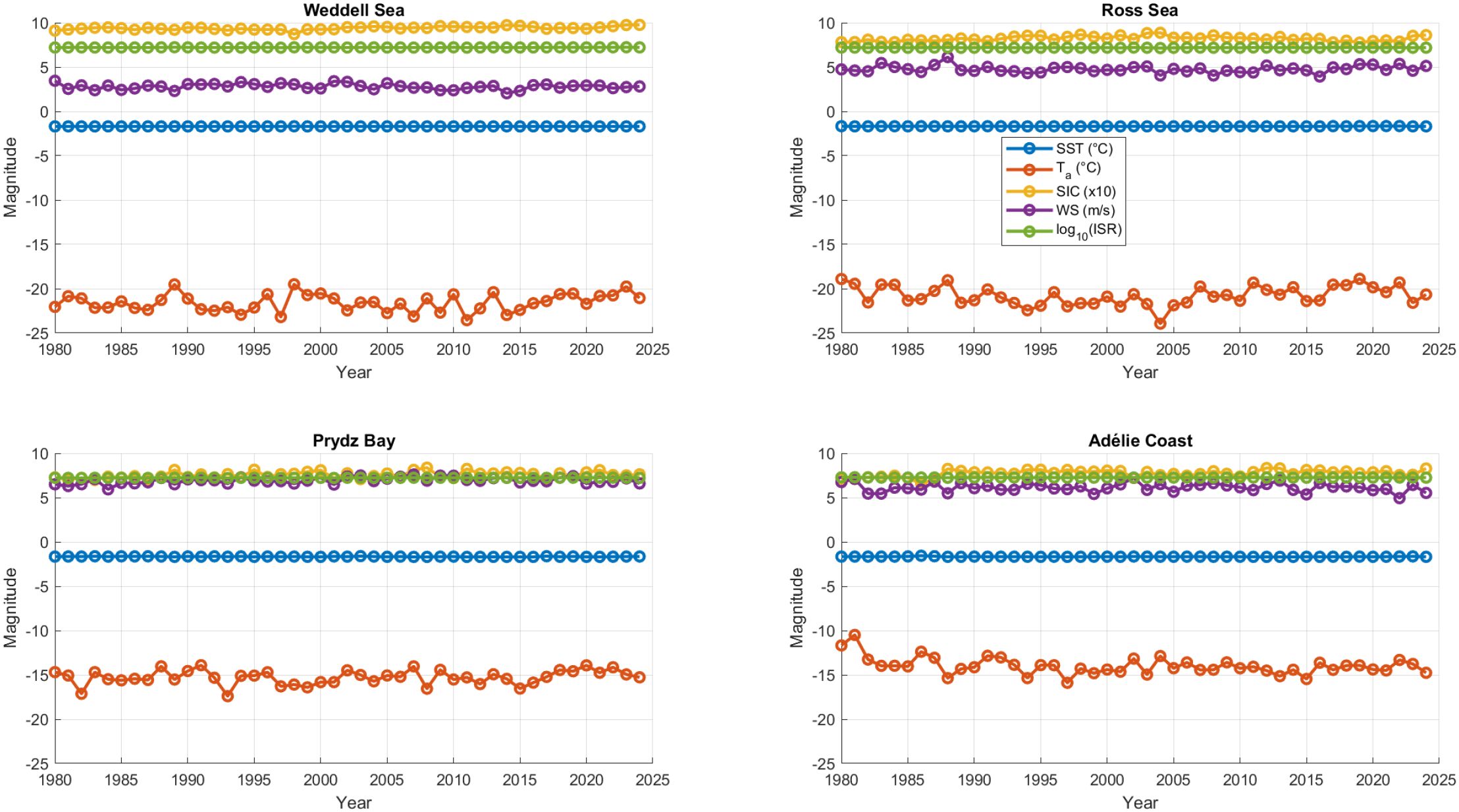
Figure 8. Annual time series of physical variables computed over dense water formation areas in the Antarctic (using data within the polygons defined by Schmidt et al. (2023). Each subplot represents one of four regions—Weddell Sea, Ross Sea, Prydz Bay, and Adélie Coast—and displays the area-weighted annual means (1980–2024) for Sea Surface Temperature (°C), Air Temperature (°C), Sea-Ice Concentration (×10), Wind Speed (m/s), and Incident Solar Radiation (log₁₀). The legend is located in the Ross Sea panel.

Wind speeds are also notably stable over time, although regional differences are evident. The Weddell Sea consistently exhibits lower wind speeds (2–3 m s⁻¹), compared to the Ross Sea, Prydz Bay, and Adélie Coast, which register higher values (5–7 m s⁻¹). T_a presents clear regional contrasts as well: in the Ross and Weddell Seas, values remain between –24 °C and –18 °C, whereas Prydz Bay and the Adélie Coast experience slightly warmer conditions, typically ranging between –17 °C and –13 °C. SIC consistently exceeds 50–60% across all regions, reaching maximum values near 100% in the Weddell Sea. These relatively stable conditions suggest that the interannual variations observed in regional heat fluxes or air–sea exchanges are primarily driven by subtle changes in atmospheric properties or by dynamic ocean-air-sea-ice interactions although they may also be influenced by several physical variables such as the interannual variability in T_a and changes in wind direction rather than wind speed.

Regarding the surface heat flux components, Figure 9 displays their annual evolution (1980–2024), spatially integrated over the same four regions, taking the output in the months from March to October. Net SWRF is consistently directed toward the ocean, with the highest values in the Adélie Coast, followed by the Ross Sea, and the lowest at Weddell Sea, and Prydz Bay. This pattern reflects differences in incident solar radiation and surface albedo, likely influenced by sea-ice cover and cloud variability.

Figure 9

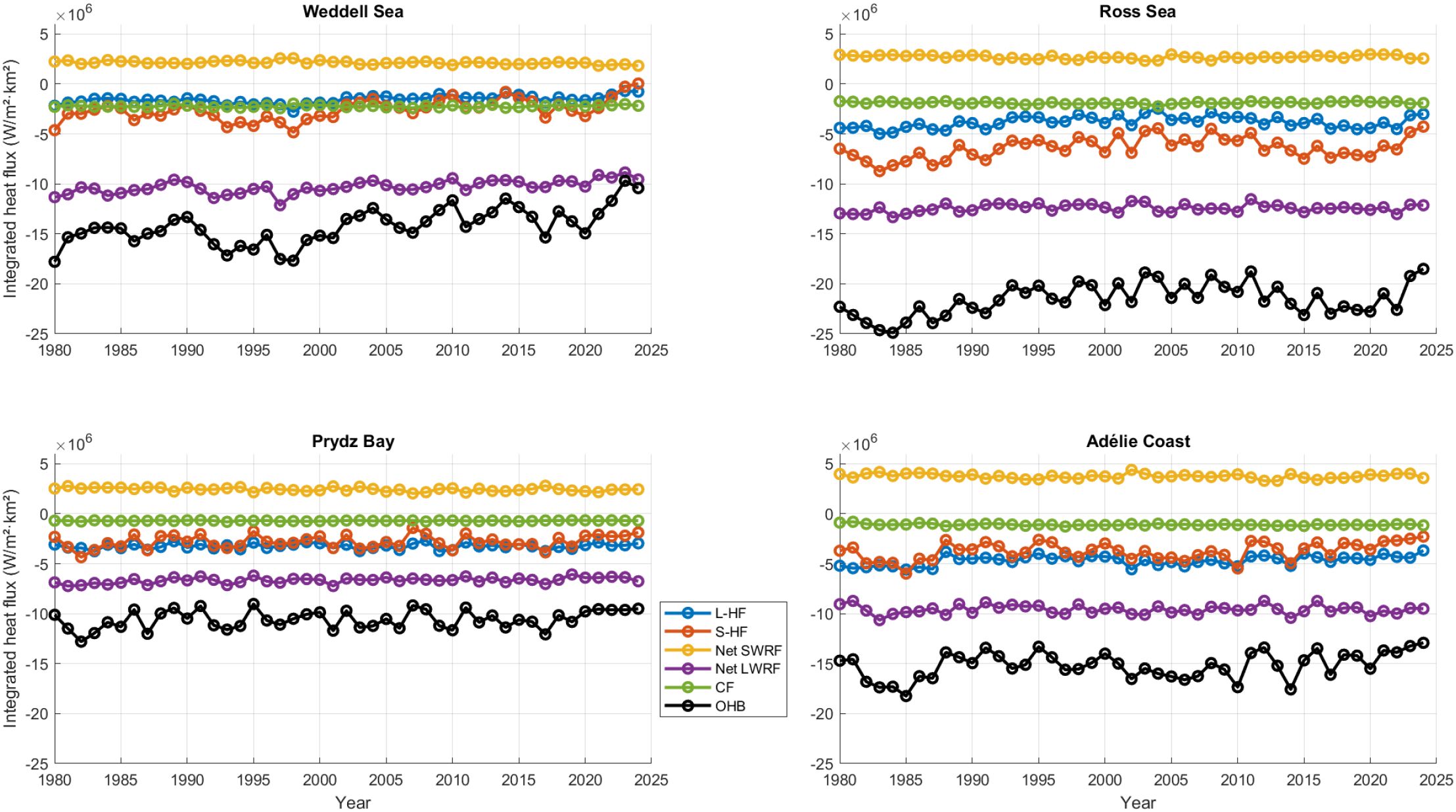
Figure 9. Annual time series of integrated heat flux components (1980–2024) computed over Antarctic dense water formation regions. Six flux components are shown—latent, sensible, shortwave net, longwave net, conductive, and total heat balance—all expressed in W m⁻² km². Each subplot corresponds to one of the four regions (Weddell Sea, Ross Sea, Prydz Bay, and Adélie Coast) with a common y-axis range from –1.5×10⁷ to 2×10⁷. Spatial integration was performed using area-weighted averaging with spherical correction within the polygons defining the dense water formation areas (Schmidt et al., 2023). The legend—displaying the flux component names and their corresponding colors—is positioned only next to the Prydz Bay panel.

All other components represent a net release of heat from the ocean to the atmosphere. Both Net LWRF and CF are relatively stable over time. Net LWRF reaches its most negative values (strongest oceanic heat loss) in the Ross Sea, followed by the Weddell Sea and Adélie Coast, and is weakest in Prydz Bay. CF is also relatively constant, particularly in regions with persistent sea-ice cover, such as the Weddell and Ross Seas.

The turbulent heat fluxes—latent and sensible—show moderate interannual variability. In the Adélie Coast and Prydz Bay, L-HF loss is slightly greater than S-HF, consistent with relatively milder air temperatures and lower relative humidity. In the Weddell Sea, both components contribute quite similarly, while in the Ross Sea, S-HF clearly exceeds L-HF, which may reflect colder, drier atmospheric conditions typical of that region, due to the frequent intrusions of very cold-dry air masses proceeding from the high continental East Antarctic plateau (Monaghan et al., 2005). Notably, a clear declining trend in S-HF appears after 2015 in the Weddell Sea, with a similar but less pronounced reduction in the Ross Sea and Adélie Coast after 2020. In Prydz Bay, however, interannual variability dominates and no robust post-2015 trend can be established.

The OHB shows that the ocean consistently loses heat to the atmosphere across all regions. Some temporal variability is observed –specially in Ross Sea and Adélie Coast up to 15-20% and 20-30%, respectively–, with a particularly notable positive trend emerging after 2015–2016, indicating a net reduction in the amount of heat released to the atmosphere. To assess the relative importance of this ocean heat loss among the regions, we compare the average heat release during a reference period (1990–2010) to the most recent two-year average (2023–2024). Even though the ice extent was unusually lower in 2022, the past two years, 2023 and 2024, have been marked by dramatically low ice cover—reaching the lowest levels observed in recent decades (Josey et al., 2024)— although this is not yet reflected by a reduction in SIC in Figure 8. Table 1 summarizes the surface heat fluxes and the relative reduction in OHB between the two periods. The Ross Sea exhibits the largest total ocean heat loss on average, followed by the Weddell Sea, Adélie Coast, and Prydz Bay; all of them experienced a reduction in ocean heat loss in 2023–2024 compared to the 1990–2010 average. The decline is strongest in the Weddell Sea (–32.0%), followed by the Adélie Coast (–14.4%), and is least pronounced in Prydz Bay (–9.8%) and the Ross Sea (–9.3%).

Table 1

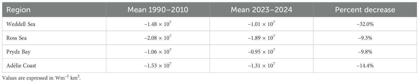
Table 1. Comparison of oceanic heat release between the 1990–2010 reference period and 2023–2024, in each Antarctic dense water formation region.

When analyzing the components of OHB, S-HF also shows a reduction in the Weddell and Ross Seas, suggesting that the observed increasing trends in 2-m air temperature observed in Figure 4 may be contributing to the reduction in S-HF and, consequently, to the overall decrease in OHB.

3.5 Shifting contributions of surface heat fluxes to OHB

In this final subsection of the results, we focus on the temporal evolution of the relative contribution of individual surface heat flux components to the ocean heat budget in the four key Antarctic regions considered (Figures 10–13). Both absolute and signed contributions are presented to distinguish between the magnitude and the direction of each component’s effect, perspective that cannot be inferred from integrated values alone. Hence, this analysis complements previous subsections revealing how the relative weight of specific heat fluxes has evolved as total ocean heat loss declined, thereby identifying which processes have become more or less influential over time.

Figure 10

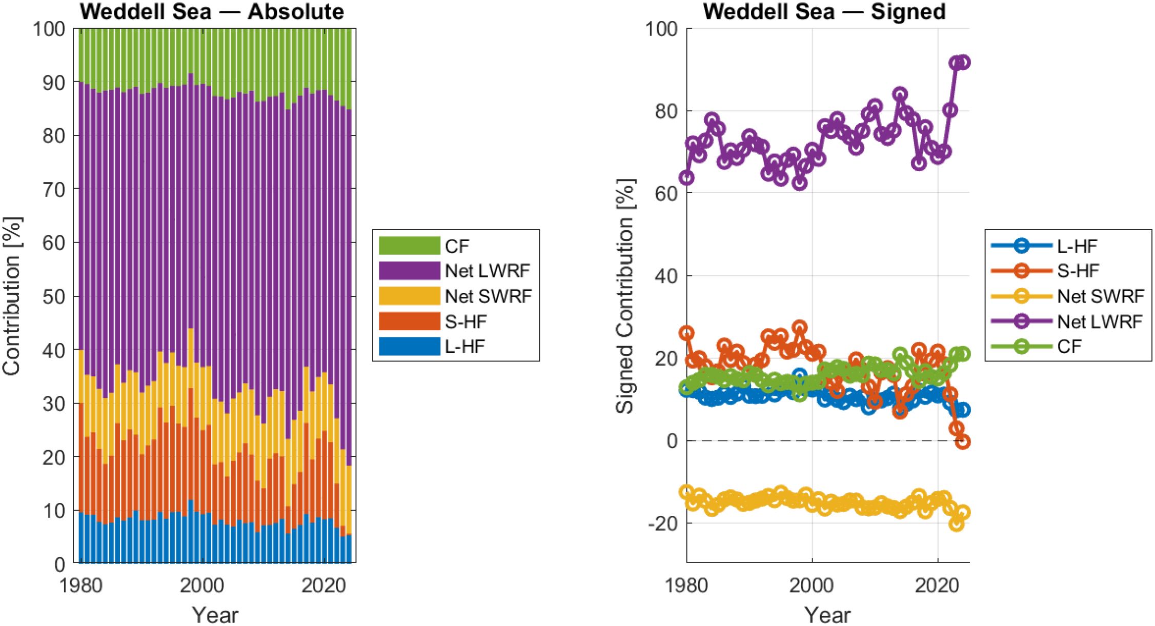
Figure 10. Relative contribution of surface heat flux components to the ocean heat budget at the Weddell Sea. The left panel shows the absolute contribution (in % of the total absolute heat budget) of each term: latent heat flux (L-HF), sensible heat flux (S-HF), net shortwave radiation (Net SWRF), net longwave radiation (Net LWRF), and conductive flux (CF). The right panel shows the signed contribution of the same components (in %) to the total heat budget, allowing the identification of net heating or cooling roles. All values are calculated over the March–October period for each year from 1980 to 2024.

Figure 11

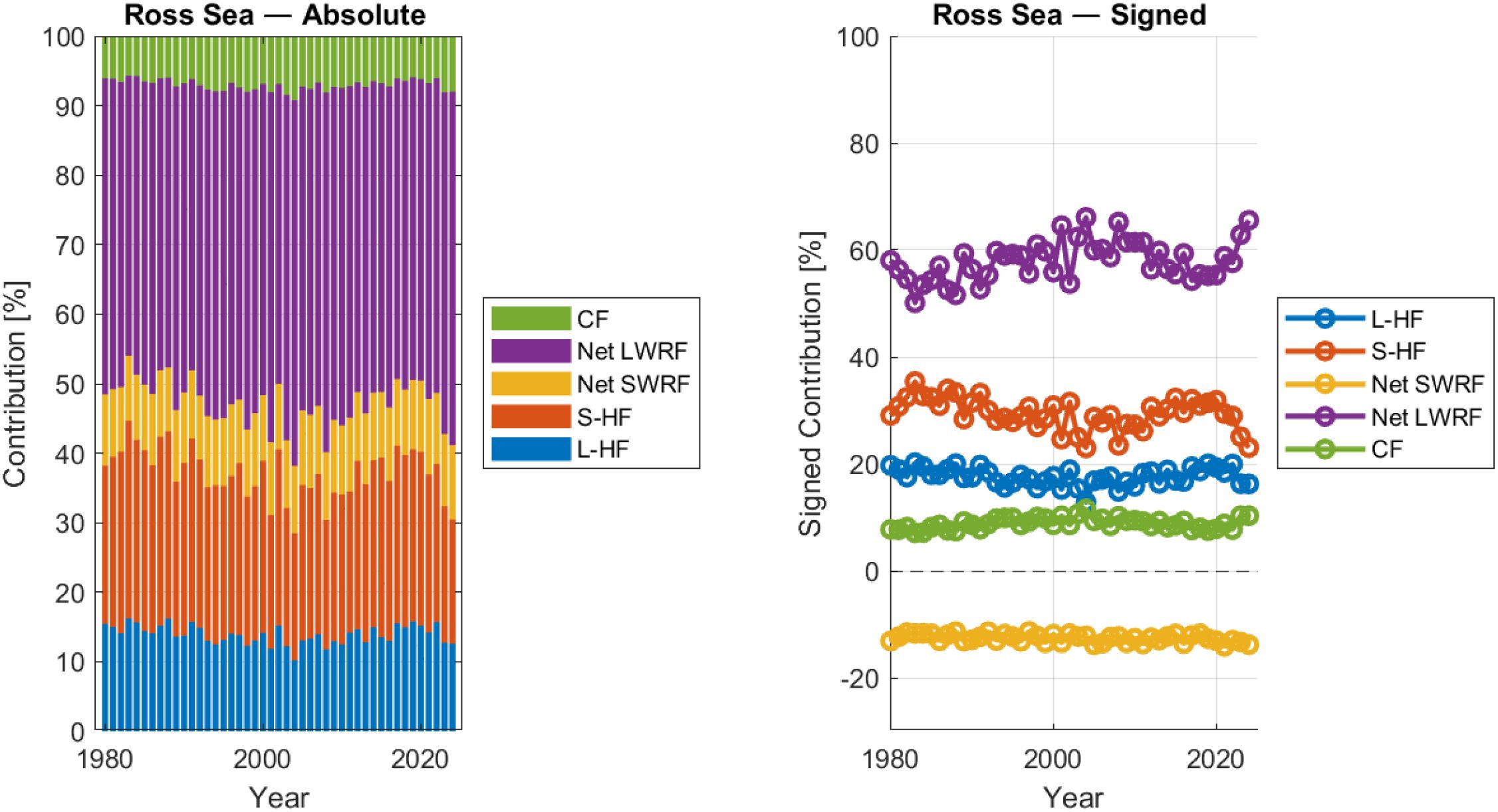
Figure 11. Relative contribution of surface heat flux components to the ocean heat budget at the Ross Sea. The left panel shows the absolute contribution (in % of the total absolute heat budget) of each term: latent heat flux (L-HF), sensible heat flux (S-HF), net shortwave radiation (Net SWRF), net longwave radiation (Net LWRF), and conductive flux (CF). The right panel shows the signed contribution of the same components (in %) to the total heat budget, allowing the identification of net heating or cooling roles. All values are calculated over the March–October period for each year from 1980 to 2024.

Figure 12

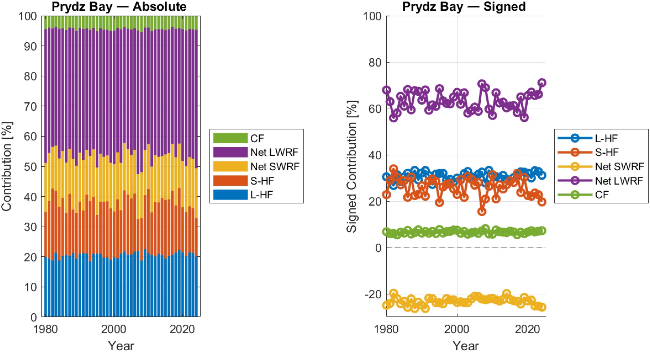
Figure 12. Relative contribution of surface heat flux components to the ocean heat budget at the Prydz Bay. The left panel shows the absolute contribution (in % of the total absolute heat budget) of each term: latent heat flux (L-HF), sensible heat flux (S-HF), net shortwave radiation (Net SWRF), net longwave radiation (Net LWRF), and conductive flux (CF). The right panel shows the signed contribution of the same components (in %) to the total heat budget, allowing the identification of net heating or cooling roles. All values are calculated over the March–October period for each year from 1980 to 2024.

Figure 13

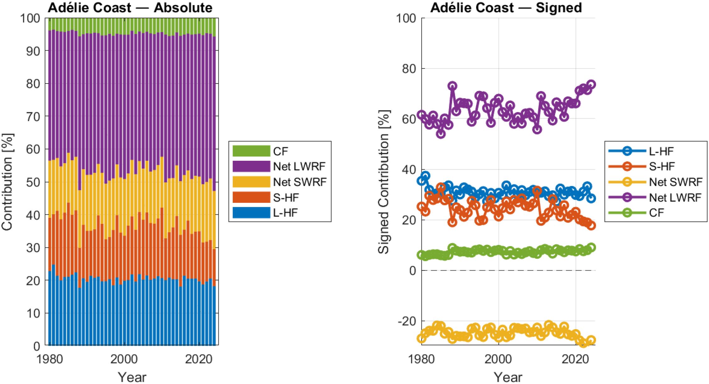
Figure 13. Relative contribution of surface heat flux components to the ocean heat budget at the Adélie Coast. The left panel shows the absolute contribution (in % of the total absolute heat budget) of each term: latent heat flux (L-HF), sensible heat flux (S-HF), net shortwave radiation (Net SWRF), net longwave radiation (Net LWRF), and conductive flux (CF). The right panel shows the signed contribution of the same components (in %) to the total heat budget, allowing the identification of net heating or cooling roles. All values are calculated over the March–October period for each year from 1980 to 2024.

Across all regions, Net LWRF consistently dominates the absolute heat budget, often exceeding half of the total energy exchange, with a consistent positive sign (warming), indicating a persistent net gain of energy from longwave processes across the seasonal ice zone. Recently, its relative contribution increases across all four regions, not because Net LWRF intensifies remaining indeed relatively stable over time, but because the total OHB has decreased.

L-HF and S-HF generally rank second in importance, displaying consistent interannual patterns throughout most of the study period. However, unlike Net LWRF, both fluxes—particularly S-HF—exhibit a gradual decrease in the final decade, declining their share in the heat budget, being especially pronounced in the Weddell and Ross Seas after 2015. A similar tendency is also observed for L-HF although less consistent across regions. The decreasing trend in these turbulent fluxes contributes to their diminishing role in the recent evolution of the surface heat exchange, in contrast to the increasingly dominant—and relatively stable—Net LWRF component.

Net SWRF remains a substantial component in absolute terms, its signed contribution shows little temporal variability, suggesting that its cooling influence has remained relatively stable over the decades. As the OHB decreases in recent years, this constancy results in a slight increase in its relative contribution, further reinforcing its role as a steady, though seasonally constrained, source of surface cooling in Antarctic waters.

CF shows a modest contribution in all regions, but it becomes relatively more relevant in the Weddell Sea, at the same level as L-HF and S-HF, where its link to seasonal sea ice dynamics and polynya activity is well established (Figure 10). Although its magnitude remains relatively stable, its relative contribution increases markedly in recent years, particularly as both L-HF and S-HF decline. In fact, in the Weddell Sea, CF surpasses S-HF—and at times even L-HF—in relative importance during the final years of the record, underscoring a shift toward ice-regulated processes as dominant contributors to surface heat exchange in this key dense water formation region.

Altogether, the signed panels reveal that while some components contribute large energy fluxes, their net effect may be partially or fully canceled by opposing terms, underscoring the importance of resolving both magnitude and sign. Beyond this compensation, the results also highlight a progressive shift in the relative weight of individual components—driven not necessarily by their own variability, but by the decline in the OHB. In particular, the increasing prominence of stable fluxes such as Net LWRF and CF in recent years reflects a reconfiguration of the surface heat exchange balance, with turbulent fluxes losing influence. These diagnostics thus provide not only a snapshot of the distinct heat exchange regimes operating in each dense water formation region, but also a window into how those regimes may evolve under ongoing global warming.

4 Discussion

This study aimed to characterize spatial and interannual variability in Antarctic surface heat fluxes and physical variables, focusing on four key dense water formation regions. Our analysis identified significant reductions in ocean–atmosphere heat exchange, particularly after 2015–2016, consistent with a weakening of thermal forcing relevant to dense water formation. While these changes may have implications for the overturning circulation, full attribution requires integrated analyses including freshwater fluxes and water-mass observations.

4.1 A physically consistent signal of declining ocean–atmosphere heat exchange

Our analysis reveals a consistent reduction in oceanic heat loss in the recent years, particularly marked in the Weddell Sea, Ross Sea, Adélie Coast, and Prydz Bay. These reductions, especially evident after 2015–2016, are primarily associated with a weakening of sensible heat fluxes, which in turn are linked to rising near-surface air temperatures. This trend reduces the thermal gradient between the atmosphere and ocean surface, thereby decreasing the efficiency of turbulent heat exchange during the austral autumn and winter months.

These observed shifts are not attributed to direct changes in solar forcing or SST, both of which remained relatively stable in our analysis, but rather to subtle atmospheric shifts, particularly the observed increase in T_a at 2m height (Figure 8). Similar atmospheric-driven processes were reported by Jullion et al. (2013), who linked freshening of exported bottom waters from the Weddell Sea to changing atmospheric conditions, including anthropogenic influences. However, the recent dramatic loss of Antarctic sea ice has substantially modified air–sea interactions in the Southern Ocean, as newly ice-free zones may serve as important sources of turbulent ocean heat loss to the atmosphere during winter (Josey et al., 2024). This may introduce a small bias in our comparison of ocean heat loss between 1990–2010 and 2023–2024 in the four selected regions, especially if sea-ice absence in one region is due to long-term decline from global warming rather than the presence of a coastal polynya. In that case, ocean heat loss in earlier years may have been greater than recent values suggest.

While we do not assess salinity or water density directly, the observed reduction in net surface heat loss—particularly in regions known to be involved in dense water production—signals a weakening in one of the key drivers of surface destabilization. Net buoyancy forcing, however, results from the combined effect of heat and freshwater fluxes. As shown by Pellichero et al. (2018), in the sea-ice sector of the Southern Ocean the meridional overturning that feeds AABW formation is primarily driven by freshwater inputs from sea-ice melt, glacial discharge, and precipitation–evaporation; surface heat exchanges modulate this freshwater-driven signal. Our results therefore provide physically consistent evidence of a shift in the thermal conditions that support bottom water formation, even though the full buoyancy forcing cannot be constrained without complementary salinity diagnostics. Further investigation integrating salinity, ocean stratification, and wind pattern analyses will be essential to fully resolve the mechanisms driving the observed decline in surface heat loss.

4.2 Regional contrasts in surface heat flux trends and their drivers

While a general reduction in heat fluxes was observed across all four sectors, important regional differences were apparent. The Ross Sea maintains the highest magnitude of oceanic heat loss, despite experiencing the smallest relative decline. This is consistent with the episodic recovery observed by Silvano et al. (2020), who linked intermittent periods of increased sea ice production and dense-water formation in the Ross Sea to specific atmospheric anomalies (positive Southern Annular Mode (SAM) and strong El Ninõ events). These episodic recoveries could partly offset the long-term declining trend in the heat budget.

In contrast, the Weddell Sea exhibited the greatest relative decrease in heat release (Table 1). This pronounced shift is consistent with reported atmospheric changes and recent warming and freshening trends in bottom waters, although we do not directly quantify water mass formation in this study. Previous studies have identified near-surface wind changes and enhanced sea-ice concentration in this region (Zhou et al., 2023) as drivers of reduced sensible heat fluxes—patterns that match those observed in our results. This northerly wind trend over the Ronne Ice Shelf favors an increase in sea-ice concentration, promoting a decreasing trend in sensible heat loss, consistent with the patterns observed in Figures 8, 9.

Fusco et al. (2018), using similar ECMWF reanalysis output, showed that oceanic heat loss in the Ross Sea reached its maximum in 2008 (-98 W m⁻²), while in the Weddell Sea it peaked in 2015 (-99 W m⁻²). Although their study only covered the 1972–2015 period, it already suggested a decreasing trend in heat loss in recent years, consistent with our results.

Prydz Bay and the Adélie Coast displayed intermediate patterns, with moderate decreases in heat fluxes. These regions experience notable wind-driven processes, with Prydz Bay characterized by strong katabatic winds, as shown in our wind-speed analysis, maintaining open water through the formation of wind-driven polynyas, which support sea-ice production, and drive ocean convection dynamics (Heywood et al., 2014; Hou and Shi, 2021). Although our study focuses on surface fluxes alone, the temporal evolution of sensible and latent heat loss in these areas provides indirect insight into changes in surface forcing that may affect dense shelf water formation.

4.3 Implications for dense water formation and the future of the MOC

The observed decline in surface ocean heat loss—particularly in regions traditionally associated with dense water production—has potential implications for AABW formation and, by extension, for the lower limb of the global MOC. Although we do not quantify dense water formation directly, the reduction in sensible and latent heat fluxes points to a weakening of one of the key surface processes that contributes to upper-ocean destabilization during the austral cold season.

These patterns are consistent with model projections suggesting that anthropogenic forcing may reduce dense shelf water production under continued atmospheric CO₂ increases (e.g., Jeong et al., 2023). If sustained, such changes in surface thermal forcing could impact the ventilation of deep ocean layers, with consequences for heat storage, oxygen distribution, and carbon sequestration. However, it is important to emphasize that these potential impacts cannot be assessed from surface fluxes alone. Full evaluation of changes in the overturning circulation requires complementary analyses of salinity, water mass properties, and transport pathways.

In this context, our results serve as an early indicator of evolving thermal conditions in Antarctic continental shelf regions. They highlight the need to integrate surface flux diagnostics with observations of water mass transformation and high-resolution coupled modeling in order to assess whether the recent changes in thermal forcing are already influencing the global overturning system.

4.4 Methodological considerations and limitations

Although ERA5 reanalysis provides robust and spatially comprehensive output from 1980 onward (Bell et al., 2021), our approach has limitations. The absence of direct measurements of salinity and comprehensive ocean density profiles prevents a complete assessment of the buoyancy-driven convective processes. As a result, our analysis is restricted to surface thermal forcing around Antarctica, without resolving the freshwater contributions that also play a critical role in driving deep convection and fully characterizing of AABW formation. Moreover, analyzing only the March–October period captures the critical dense water formation season but may overlook subtle yet significant summer changes. Additionally, and according to Schmidt et al. (2023), the free-ice open water area, i.e., coastal polynya formation, occurs during different months depending on the region: in Prydz Bay, it spans from April to June; along the Adélie Coast, it extends from April to September; and in the Ross Sea, it also occurs from April to June. However, recent studies suggest that the period of sea ice and coastal polynyas formation is shifting later in the season (Fraser et al., 2012; Josey et al., 2024). Moreover, while our analysis effectively captures large-scale spatial trends and temporal variability, small-scale processes crucial for DSW formation (such as coastal polynyas, tidal-driven mixing, or iceberg calving events) were only indirectly considered (Heywood et al., 2014; Holland et al., 2020; Menezes et al., 2017).

The inherent uncertainties in reanalysis datasets, especially regarding surface fluxes and sea-ice processes, also necessitate caution. Moreover, Truong et al. (2022) and Mallet et al. (2023) reported biases in the thermodynamic structure of the lower troposphere and in the specific humidity due to deficiencies in simulating cloud cover and water content in the ERA5 reanalysis over the high latitudes of Southern Ocean.

4.5 Perspectives and future work

Future research should address key gaps identified in this study. Incorporating salinity-related processes—such as brine rejection, initial mixed-layer salinity, and monthly salinity changes—would improve assessment of the salt budget and its role in dense shelf water formation, as shown by Portela et al. (2022). Expanding subsurface ocean observations through gliders, Argo floats (Heywood et al., 2014; Johnson and Purkey, 2024), and instrumented marine mammals—particularly southern elephant seals, which are effective samplers of Antarctic coastal polynyas during winter (Roquet et al., 2014; Labrousse et al., 2018; Malpress et al., 2017)—would further enhance the characterization of density and buoyancy changes needed to validate trends in dense water formation. In parallel, high-resolution coupled ocean–ice–atmosphere models are needed to explore the nonlinear interactions between surface forcing, sea-ice dynamics, and ocean stratification. Such models can also simulate scenarios of changing atmospheric and cryospheric conditions to assess the sensitivity of ice-shelf processes to ongoing climatic shifts.

Additionally, assessing freshwater fluxes from melting ice shelves and icebergs, and their oceanic impacts (Holland et al., 2020; Olivé Abelló et al., 2025; Sohail et al., 2025) is crucial for improved understanding of future trends. Finally, integrating climate model projections (CMIP6) to explore future scenarios of Antarctic dense water formation and global overturning circulation would significantly complement the observational and reanalysis-based approaches presented here.

5 Conclusions

This study analyzed ocean–atmosphere heat fluxes over the Southern Ocean south of 60°S using ERA5 monthly reanalysis output from March to October for the period 1980–2024, focusing specifically on the four main dense water formation regions: the Weddell Sea, Ross Sea, Prydz Bay, and Adélie Coast. The analysis allowed us to quantify long-term trends and interannual variability in surface heat fluxes and associated physical variables to characterize changes in surface thermal forcing. There is a consistent, regionally varying reduction in the OHB, indicating decreased oceanic heat loss to the atmosphere, especially after the mid-2010s. Between the reference period (1990–2010) and recent years (2023–2024), the reduction in oceanic heat loss was most pronounced in the Weddell Sea (–32.0%) and Adélie Coast (–14.4%), moderate in Prydz Bay (–9.8%), and relatively small in the Ross Sea (–9.3%).

The reduction in OHB across these regions is mainly attributed to a decreased S-HF, consistent with observed positive trends in air temperature at 2-m height. This warming in the near-surface atmosphere was particularly notable around the Antarctic Peninsula, Bellingshausen Sea, Amundsen Sea, and certain sectors of the Indian Ocean. For example, the Ross Sea experienced air temperature increases of up to 0.2 °C per decade, contributing to a measurable decline in heat loss and consequent stabilization of surface waters. These atmospheric warming trends have directly reduced vertical thermal gradients, diminishing turbulent heat exchanges between the ocean and atmosphere.

Sea surface temperature remained stable throughout the analyzed period (1980–2024), predominantly near the freezing point. Likewise, incident solar radiation did not show significant changes, suggesting that variations in ocean–atmosphere heat fluxes and subsequent dense water formation are predominantly driven by atmospheric processes (temperature and winds) rather than by direct solar or ocean surface thermal forcing.

Regional contrasts were observed in both the magnitude and variability of the fluxes. The Ross Sea consistently exhibited the strongest heat loss (typically around –100 W m⁻² nearshore), confirming its role as a zone of intense surface cooling, although the relative decline was more modest. In comparison, the Weddell Sea (∼-50 W m⁻²) and Adélie Coast (∼-30 W m⁻²) displayed intermediate heat losses, while Prydz Bay demonstrated moderate values (∼-40 to -60 W m⁻²). These contrasts highlight the heterogeneous response of Antarctic shelf regions to atmospheric forcing and reinforce the importance of local dynamics—such as polynya activity and wind regimes—in modulating surface thermal conditions.

Sea-ice concentration, generally high and stable in all four regions (frequently above 60%, approaching 100% in the Weddell Sea), did not exhibit major temporal trends during the analysis period. However, even subtle variations in sea-ice coverage and associated conductive fluxes were consistent with observed patterns of reduced oceanic heat loss. Particularly, a negative correlation was observed between conductive flux trends and 2-m air temperature, reflecting the role of atmospheric warming in decreasing ice–ocean temperature gradients. Warmer air reduces the vertical temperature contrast that drives conduction through sea ice, thereby decreasing the conductive flux.

Methodologically, using ERA5 reanalysis provided robust, spatially extensive, and temporally consistent datasets, overcoming observational limitations at high southern latitudes. Nevertheless, the absence of direct salinity and subsurface water density profiles implies that our conclusions would benefit from additional validation through direct observational studies or complementary numerical modeling. Future work incorporating direct ocean measurements, buoyancy-driven convection trends and high-resolution modeling would significantly enhance confidence in these findings.

While we do not directly evaluate salinity or dense water formation, the trends identified in surface thermal forcing provide physically consistent evidence of changing boundary conditions that may influence dense water formation processes. The use of reanalysis-based diagnostics, particularly when integrated over time and space, offers a valuable means to monitor surface energy exchange in regions where in situ data remain scarce. These diagnostics, while limited in scope, contribute to our understanding of how climate variability and long-term atmospheric changes may affect the dynamics of the Southern Ocean.

Data availability statement

Publicly available datasets were analyzed in this study. This data can be found here: https://cds.climate.copernicus.eu/.

Author contributions

FM: Conceptualization, Investigation, Data curation, Methodology, Visualization, Formal analysis, Writing – original draft. AOA: Writing – review & editing, Methodology, Conceptualization.

Funding

The author(s) declare that no financial support was received for the research and/or publication of this article.

Acknowledgments

The authors gratefully acknowledge the European Centre for Medium-Range Weather Forecasts (ECMWF) and the Copernicus Climate Data Store for providing the ERA5 reanalysis output. The authors are very grateful to the editor, Dr. Donglai Gong, and to the two reviewers, Dr. Christina Schmidt and Dr. Felipe Vilela-Silva, for their many valuable comments and suggestions.

Conflict of interest

The authors declare that the research was conducted in the absence of any commercial or financial relationships that could be construed as a potential conflict of interest. The author(s) declared that they were an editorial board member of Frontiers, at the time of submission. This had no impact on the peer review process and the final decision.

Generative AI statement

The author(s) declare that Generative AI was used in the creation of this manuscript. The authors used generative AI tools (e.g., ChatGPT) to assist with language refinement and editorial suggestions during the manuscript preparation. All scientific content, analyses, and final text were written and verified by the authors, who take full responsibility for the work.

Any alternative text (alt text) provided alongside figures in this article has been generated by Frontiers with the support of artificial intelligence and reasonable efforts have been made to ensure accuracy, including review by the authors wherever possible. If you identify any issues, please contact us.

Publisher’s note

All claims expressed in this article are solely those of the authors and do not necessarily represent those of their affiliated organizations, or those of the publisher, the editors and the reviewers. Any product that may be evaluated in this article, or claim that may be made by its manufacturer, is not guaranteed or endorsed by the publisher.

Supplementary material

The Supplementary Material for this article can be found online at: https://www.frontiersin.org/articles/10.3389/fmars.2025.1644717/full#supplementary-material

References

Abernathey R. P., Cerovecki I., Holland P. R., Newsom E., Mazloff M., and Talley L. D. (2016). Water-mass transformation by sea ice in the upper branch of the southern ocean overturning. Nat. Geosci. 9, 596–601. doi: 10.1038/ngeo2749

Crossref Full Text | Google Scholar

Azaneu M., Kerr R., Mata M. M., and Garcia C. A. (2013). Trends in the deep Southern Ocean, (1958–2010): Implications for Antarctic Bottom Water properties and volume export. J. Geophysical Research: Oceans 118, 4213–4227. doi: 10.1002/jgrc.20303

Crossref Full Text | Google Scholar

Bell B., Hersbach H., Simmons A., Berrisford P., Dahlgren P., Horányi A., et al. (2021). The ERA5 global reanalysis: Preliminary extension to 1950. Q. J. R. Meteorological Soc. 147, 4186–4227. doi: 10.1002/qj.4174

Crossref Full Text | Google Scholar

Broecker W. S. (1987). Unpleasant surprises in the greenhouse? Nature 328, 123–126. doi: 10.1038/328123a0

Crossref Full Text | Google Scholar

Budillon G., Castagno P., Aliani S., Spezie G., and Padman L. (2011). Thermohaline variability and Antarctic bottom water formation at the Ross Sea shelf break. Deep Sea Res. Part I: Oceanographic Res. Papers 58, 1002–1018. doi: 10.1016/j.dsr.2011.07.002

Crossref Full Text | Google Scholar

Budillon G., Fusco G., and Spezie G. (2000). A study of surface heat fluxes in the Ross Sea (Antarctica). Antarctic Sci. 12, 243–254. doi: 10.1017/S0954102000000298

Crossref Full Text | Google Scholar

Caton Harrison T., King J. C., Bracegirdle T. J., and Lu H. (2024). Dynamics of extreme wind events in the marine and terrestrial sectors of coastal Antarctica. Q. J. R. Meteorological Soc. 150, 2646–2666. doi: 10.1002/qj.4727

Crossref Full Text | Google Scholar

De Lavergne C., Madec G., Le Sommer J., Nurser A. G., and Naveira Garabato A. C. (2016). On the consumption of Antarctic Bottom Water in the abyssal ocean. J. Phys. Oceanography 46, 635–661. doi: 10.1175/JPO-D-14-0201.1

Crossref Full Text | Google Scholar

Dong X., Wang Y., Hou S., Ding M., Yin B., and Zhang Y. (2020). Robustness of the recent global atmospheric reanalyses for antarctic near-surface wind speed climatology. J. Climate 33, 4027–4043. doi: 10.1175/JCLI-D-19-0648.1

Crossref Full Text | Google Scholar

ECMWF (2024). IFS Documentation CY49R1 - Part IV: Physical Processes (Reading, United KIngdom: ECMWF). chap. 4. doi: 10.21957/c731ee1102

Crossref Full Text | Google Scholar

Fraser A. D., Massom R. A., Michael K. J., Galton-Fenzi B. K., and Lieser J. L. (2012). East antarctic landfast sea ice distribution and variability 2000–08. J. Climate 25, 1137–1156. doi: 10.1175/JCLI-D-10-05032.1

Crossref Full Text | Google Scholar

Fusco G., Budillon G., and Spezie G. (2009). Surface heat fluxes and thermohaline variability in the Ross Sea and in Terra Nova Bay polynya. Continental Shelf Res. 29, 1887–1895. doi: 10.1016/j.csr.2009.07.006

Crossref Full Text | Google Scholar

Fusco G., Cotroneo Y., and Aulicino G. (2018). Different behaviours of the ross and weddell seas surface heat fluxes in the period 1972–2015. Climate 6, 17. doi: 10.3390/cli6010017

Crossref Full Text | Google Scholar

Golledge N. R., Keller E. D., Gossart A., Malyarenko A., Bahamondes-Dominguez A., Krapp M., et al. (2025). Antarctic coastal polynyas in the global climate system. Nat. Rev. Earth Environ. 6, 126–139. doi: 10.1038/s43017-024-00634-x

Crossref Full Text | Google Scholar

Gunn K. L., Rintoul S. R., England M. H., and Bowen M. M. (2023). Recent reduced abyssal overturning and ventilation in the Australian Antarctic Basin. Nat. Climate Change 13, 537–544. doi: 10.1038/s41558-023-01667-8

Crossref Full Text | Google Scholar

Gurjão C. D., Pezzi L. P., Parise C. K., Justino F. B., Carpenedo C. B., Schumacher V., et al. (2025). Atmospheric variability and sea-ice changes in the southern hemisphere. Atmosphere 16, 284. doi: 10.3390/atmos16030284

Crossref Full Text | Google Scholar

Hersbach H., Bell B., Berrisford P., Hirahara S., Horányi A., Muñoz-Sabater J., et al. (2020). The ERA5 global reanalysis. Q. J. R. meteorological Soc. 146, 1999–2049. doi: 10.1002/qj.3803

Crossref Full Text | Google Scholar

Heuzé C. (2020). Antarctic bottom water and North Atlantic deep water in CMIP6 models. Ocean Sci. Discussions 2020, 1–38. doi: 10.5194/os-17-59-2021

Crossref Full Text | Google Scholar

Heywood K. J., Schmidtko S., Heuzé C., Kaiser J., Jickells T. D., Queste B. Y., et al. (2014). Ocean processes at the Antarctic continental slope. Philos. Trans. R. Soc. A: Mathematical Phys. Eng. Sci. 372, 20130047. doi: 10.1098/rsta.2013.0047

PubMed Abstract | Crossref Full Text | Google Scholar

Holland D. M., Nicholls K. W., and Basinski A. (2020). The southern ocean and its interaction with the Antarctic ice sheet. Science 367, 1326–1330. doi: 10.1126/science.aaz5491

PubMed Abstract | Crossref Full Text | Google Scholar

Holzer M., DeVries T., and de Lavergne C. (2021). Diffusion controls the ventilation of a Pacific Shadow Zone above abyssal overturning. Nat. Commun. 12, 4348. doi: 10.1038/s41467-021-24648-x

PubMed Abstract | Crossref Full Text | Google Scholar

Hou S. and Shi J. (2021). Variability and formation mechanism of polynyas in eastern Prydz Bay, Antarctica. Remote Sens. 13, 5089. doi: 10.3390/rs13245089

Crossref Full Text | Google Scholar

Jacobs S. S., Amos A. F., and Bruchhausen P. M. (1970). “Ross Sea oceanography and Antarctic bottom water formation,” in Deep Sea Research and Oceanographic Abstracts, vol. 17. (Elsevier), 935–962. doi: 10.1016/0011-7471(70)90046-X

Crossref Full Text | Google Scholar

Jeong H., Lee S.-S., Park H.-S., and Stewart A. L. (2023). Future changes in Antarctic coastal polynyas and bottom water formation simulated by a high-resolution coupled model. Commun. Earth Environ. 4, 490. doi: 10.1038/s43247-023-01156-y

Crossref Full Text | Google Scholar

Johnson G. C. (2008). Quantifying Antarctic bottom water and North Atlantic deep water volumes. J. Geophysical Research: Oceans 113. doi: 10.1029/2007JC004477

Crossref Full Text | Google Scholar

Johnson G. C. and Purkey S. G. (2024). Refined estimates of global ocean deep and abyssal decadal warming trends. Geophysical Res. Lett. 51, e2024GL111229. doi: 10.1029/2024GL111229

Crossref Full Text | Google Scholar

Josey S. A., Meijers A. J., Blaker A. T., Grist J. P., Mecking J., and Ayres H. C. (2024). Record low antarctic sea ice in 2023 increased ocean heat loss and storms. Nature 636, 635–639. doi: 10.1038/s41586-024-08368-y

PubMed Abstract | Crossref Full Text | Google Scholar

Jullion L., Naveira Garabato A. C., Meredith M. P., Holland P. R., Courtois P., and King B. A. (2013). Decadal freshening of the Antarctic Bottom Water exported from the Weddell Sea. J. Climate 26, 8111–8125. doi: 10.1175/JCLI-D-12-00765.1

Crossref Full Text | Google Scholar

Labrousse S., Williams G., Tamura T., Bestley S., Sallée J.-B., Fraser A. D., et al. (2018). Coastal polynyas: Winter oases for subadult southern elephant seals in East Antarctica. Sci. Rep. 8, 3183. doi: 10.1038/s41598-018-21388-9

PubMed Abstract | Crossref Full Text | Google Scholar

Lago V. and England M. H. (2019). Projected slowdown of Antarctic Bottom Water formation in response to amplified meltwater contributions. J. Climate 32, 6319–6335. doi: 10.1175/JCLI-D-18-0622.1

Crossref Full Text | Google Scholar

Lee S.-K., Lumpkin R., Gomez F., Yeager S., Lopez H., Takglis F., et al. (2023). Human-induced changes in the global meridional overturning circulation are emerging from the Southern Ocean. Commun. Earth Environ. 4, 69. doi: 10.1038/s43247-023-00727-3

Crossref Full Text | Google Scholar

Mallet M. D., Alexander S. P., Protat A., and Fiddes S. L. (2023). Reducing Southern Ocean shortwave radiation errors in the ERA5 reanalysis with machine learning and 25 years of surface observations. Artif. Intell. Earth Syst. 2, e220044. doi: 10.1175/AIES-D-22-0044.1

Crossref Full Text | Google Scholar

Malpress V., Bestley S., Corney S., Welsford D., Labrousse S., Sumner M., et al. (2017). Bio-physical characterisation of polynyas as a key foraging habitat for juvenile male southern elephant seals (mirounga leonina) in prydz bay, east Antarctica. PloS One 12, e0184536. doi: 10.1371/journal.pone.0184536

PubMed Abstract | Crossref Full Text | Google Scholar

Marshall J. and Speer K. (2012). Closure of the meridional overturning circulation through Southern Ocean upwelling. Nat. Geosci. 5, 171–180. doi: 10.1038/ngeo1391

Crossref Full Text | Google Scholar

Menezes V. V., Macdonald A. M., and Schatzman C. (2017). Accelerated freshening of Antarctic Bottom Water over the last decade in the Southern Indian Ocean. Sci. Adv. 3, e1601426. doi: 10.1126/sciadv.1601426

PubMed Abstract | Crossref Full Text | Google Scholar

Meredith M. P., Jullion L., Brown P. J., Naveira Garabato A. C., and Couldrey M. P. (2014). Dense waters of the Weddell and Scotia Seas: recent changes in properties and circulation. Philos. Trans. R. Soc. A: Mathematical Phys. Eng. Sci. 372, 20130041. doi: 10.1098/rsta.2013.0041

PubMed Abstract | Crossref Full Text | Google Scholar

Meredith M. P., Locarnini R. A., Van Scoy K. A., Watson A. J., Heywood K. J., and King B. A. (2000). On the sources of Weddell Gyre Antarctic bottom water. J. Geophysical Research: Oceans 105, 1093–1104. doi: 10.1029/1999JC900263

Crossref Full Text | Google Scholar

Monaghan A. J., Bromwich D. H., Powers J. G., and Manning K. W. (2005). The climate of the mcmurdo, Antarctica, region as represented by one year of forecasts from the antarctic mesoscale prediction system. J. Climate 18, 1174–1189. doi: 10.1175/JCLI3336.1

Crossref Full Text | Google Scholar

Nakata K., Ohshima K. I., and Nihashi S. (2019). Estimation of thin-ice thickness and discrimination of ice type from amsr-e passive microwave data. IEEE Trans. Geosci. Remote Sens. 57, 263–276. doi: 10.1109/TGRS.2018.2853590

Crossref Full Text | Google Scholar

Nakata K., Ohshima K., and Nihashi S. (2021). Mapping of active frazil for antarctic coastal polynyas, with an estimation of sea-ice production. Geophysical Res. Lett. 48, e2020GL091353. doi: 10.1029/2020GL091353

Crossref Full Text | Google Scholar

Naveira Garabato A. C., Zika J. D., Jullion L., Brown P. J., Holland P. R., Meredith M. P., et al. (2016). The thermodynamic balance of the weddell gyre. Geophysical Res. Lett. 43, 317–325. doi: 10.1002/2015GL066658

Crossref Full Text | Google Scholar

Newsom E. R., Bitz C. M., Bryan F. O., Abernathey R., and Gent P. R. (2016). Southern ocean deep circulation and heat uptake in a high-resolution climate model. J. Climate 29, 2597–2619. doi: 10.1175/JCLI-D-15-0513.1

Crossref Full Text | Google Scholar

Ohshima K. I., Fukamachi Y., Williams G. D., Nihashi S., Roquet F., Kitade Y., et al. (2013). Antarctic Bottom Water production by intense sea-ice formation in the Cape Darnley polynya. Nat. Geosci. 6, 235–240. doi: 10.1038/ngeo1738

Crossref Full Text | Google Scholar

Olivé-Abelló A., Pelegrí J., Haumann F., and Machín F. (2024). Dominant biogeochemical processes in the Scotia Sea revealed by an inverse box model. Authorea Preprints. doi: 10.22541/essoar.173557595.54433895/v1

Crossref Full Text | Google Scholar

Olivé-Abelló A., Mathiot P., Jourdain N. C., Kostov Y., Holland P. R., Gascoin S., et al (2025). Iceberg grounding enhances the release of freshwater on the Antarctic continentalshelf. Journal of Geophysical Research: Oceans. 130, e2025JC022857. doi: 10.1029/2025JC022857

Crossref Full Text | Google Scholar

Orsi A. H., Johnson G. C., and Bullister J. L. (1999). Circulation, mixing, and production of Antarctic Bottom Water. Prog. Oceanography 43, 55–109. doi: 10.1016/S0079-6611(99)00004-X

Crossref Full Text | Google Scholar

Orsi A. H., Smethie W. M. Jr., and Bullister J. L. (2002). On the total input of Antarctic waters to the deep ocean: A preliminary estimate from chlorofluorocarbon measurements. J. Geophysical Research: Oceans 107, 31–31. doi: 10.1029/2001JC000976

Crossref Full Text | Google Scholar

Pellichero V., Sallée J.-B., Chapman C. C., and Downes S. M. (2018). The southern ocean meridional overturning in the sea-ice sector is driven by freshwater fluxes. Nat. Commun. 9, 1789. doi: 10.1038/s41467-018-04101-2

PubMed Abstract | Crossref Full Text | Google Scholar

Portela E., Rintoul S. R., Herraiz-Borreguero L., Roquet F., Bestley S., Van Wijk E., et al. (2022). Controls on dense shelf water formation in four east antarctic polynyas. J. Geophysical Research: Oceans 127, e2022JC018804. doi: 10.1029/2022JC018804

Crossref Full Text | Google Scholar

Purkey S. G. and Johnson G. C. (2012). Global contraction of Antarctic bottom water between the 1980s and 2000s. J. Climate 25, 5830–5844. doi: 10.1175/JCLI-D-11-00612.1

Crossref Full Text | Google Scholar

Rahmstorf S. (2002). Ocean circulation and climate during the past 120,000 years. Nature 419, 207–214. doi: 10.1038/nature01090

PubMed Abstract | Crossref Full Text | Google Scholar

Renfrew I. A., King J. C., and Markus T. (2002). Coastal polynyas in the southern weddell sea: Variability of the surface energy budget. J. Geophysical Research: Oceans 107, 16–11. doi: 10.1029/2000JC000720

Crossref Full Text | Google Scholar

Roquet F., Williams G., Hindell M. A., Harcourt R., McMahon C., Guinet C., et al. (2014). A southern Indian ocean database of hydrographic profiles obtained with instrumented elephant seals. Sci. Data 1, 1–10. doi: 10.1038/sdata.2014.28

PubMed Abstract | Crossref Full Text | Google Scholar

Sarmiento J. L., Gruber N., Brzezinski M. A., and Dunne J. P. (2004). High-latitude controls of thermocline nutrients and low latitude biological productivity. Nature 427 (6969), 56–60.

PubMed Abstract | Google Scholar

Schmidt C., Morrison A. K., and England M. H. (2023). Wind–and sea-ice–driven interannual variability of Antarctic Bottom water formation. J. Geophysical Research: Oceans 128, e2023JC019774. doi: 10.1029/2023JC019774

Crossref Full Text | Google Scholar

Seabrooke J. M., Hufford G. L., and Elder R. B. (1971). Formation of Antarctic bottom water in the Weddell Sea. J. Geophysical Res. 76, 2164–2178. doi: 10.1029/JC076i009p02164

Crossref Full Text | Google Scholar

Semtner A. J. Jr. (1976). A model for the thermodynamic growth of sea ice in numerical investigations of climate. J. Phys. Oceanography 6, 379–389. doi: 10.1175/1520-0485(1976)006<0379:AMFTTG>2.0.CO;2

Crossref Full Text | Google Scholar

Silvano A., Foppert A., Rintoul S. R., Holland P. R., Tamura T., Kimura N., et al. (2020). Recent recovery of Antarctic Bottom Water formation in the Ross Sea driven by climate anomalies. Nat. Geosci. 13. doi: 10.3389/fmars.2023.1221701

Crossref Full Text | Google Scholar

Silvano A., Purkey S., Gordon A. L., Castagno P., Stewart A. L., Rintoul S. R., et al. (2023). Observing Antarctic bottom water in the Southern Ocean. Front. Mar. Sci. 10, 1221701. doi: 10.1038/s41561-020-00655-3

Crossref Full Text | Google Scholar

Sohail T., Gayen B., and Klocker A. (2025). Decline of antarctic circumpolar current due to polar ocean freshening. Environ. Res. Lett. 20. doi: 10.1088/1748-9326/adb31c

Crossref Full Text | Google Scholar

Stommel H. (1966). The Gulf Stream: a physical and dynamical description (Berkeley, USA: Univ of California Press). doi: 10.5962/bhl.title.34897

Crossref Full Text | Google Scholar

Tamura T., Ohshima K. I., Fraser A. D., and Williams G. D. (2016). Sea ice production variability in antarctic coastal polynyas. J. Geophysical Research: Oceans 121, 2967–2979. doi: 10.1002/2015JC011537

Crossref Full Text | Google Scholar

Thompson A. F. and Youngs M. K. (2013). Surface exchange between the Weddell and Scotia seas. Geophysical Res. Lett. 40, 5920–5925. doi: 10.1002/2013GL058114

Crossref Full Text | Google Scholar

Truong S. C., Huang Y., Siems S. T., Manton M. J., and Lang F. (2022). Biases in the thermodynamic structure over the Southern Ocean in ERA5 and their radiative implications. Int. J. Climatology 42, 7685–7702. doi: 10.1002/joc.7672

Crossref Full Text | Google Scholar

Williams G. D., Aoki S., Jacobs S., Rintoul S., Tamura T., and Bindoff N. (2010). Antarctic bottom water from the Adélie and George V land coast, east Antarctica (140–149 E). J. Geophysical Research: Oceans 115. doi: 10.1029/2009JC005812

Crossref Full Text | Google Scholar

Williams G., Bindoff N., Marsland S., and Rintoul S. (2008). Formation and export of dense shelf water from the adélie depression, east Antarctica. J. Geophysical Research: Oceans 113. doi: 10.1029/2007JC004346

Crossref Full Text | Google Scholar

Williams G., Herraiz-Borreguero L., Roquet F., Tamura T., Ohshima K., Fukamachi Y., et al. (2016). The suppression of Antarctic bottom water formation by melting ice shelves in Prydz Bay. Nat. Commun. 7, 12577. doi: 10.1038/ncomms12577

PubMed Abstract | Crossref Full Text | Google Scholar

Zhang Z., Xie C., Castagno P., England M. H., Wang X., Dinniman M. S., et al. (2024). Evidence for large-scale climate forcing of dense shelf water variability in the ross sea. Nat. Commun. 15, 8190. doi: 10.1038/s41467-024-52524-x

PubMed Abstract | Crossref Full Text | Google Scholar

Zhou S., Meijers A. J., Meredith M. P., Abrahamsen E. P., Holland P. R., Silvano A., et al. (2023). Slowdown of Antarctic Bottom Water export driven by climatic wind and sea-ice changes. Nat. Climate Change 13, 701–709. doi: 10.1038/s41558-023-01695-4

Crossref Full Text | Google Scholar