Wind-stress misalignment in the presence of swells in the Bay of Bengal

This study investigates the directional characteristics of momentum flux, τ, under diverse wind-wave conditions in the Bay of Bengal (BoB). Using high-frequency data from an eddy covariance flux system deployed on a moored buoy, we identify various cases of wind-swell alignment and their resulting τ directions, with emphasis on seasonal variations. During June-August (JJA), when winds and swells are generally aligned, τ lies between wind and swell directions in 34% of wind-dominated cases, facilitating momentum transfer to developing seas. However, in 57% of cases where swells dominate or winds weaken, τ shifts toward the swell direction. In December-February (DJF), counter-swell conditions with moderate winds dominate, aligning τ between wind and opposing swell directions under wind dominance or between wind and swell directions when swells dominate. For the first time, this study quantifies the biases in Monin-Obukhov Similarity Theory (MOST)-based bulk flux models, which underestimate stress by ~12% under counter-swell conditions and ~7% in swell-dominated regimes due to their inability to account accurately the sea-state effects. These findings highlight the key role of wind-swell misalignment and swell-induced stresses in modulating τ direction and magnitude. Our results emphasize the need for parameterizations that account more accurately the sea-state effects to improve air-sea interaction models in seasonally wind-reversing, swell-dominated regions like the BoB.

1 Introduction

Accurate estimation of the momentum flux ($\text{τ}$), is crucial as it plays a fundamental role in various air-sea interaction processes, including the generation of surface waves, and currents, development of the oceanic mixed layer and large-scale atmospheric and oceanic circulation patterns (Cronin et al., 2019). $\text{τ}$ results from the turbulent exchanges between winds and ocean surface waves, and can be measured directly using eddy covariance methods (Edson et al., 1998; Hanley and Belcher, 2008). However, measurement challenges such as platform motion correction and flow distortion (Edson et al., 1998), and the inability to completely resolve the near-surface turbulence (Husain et al., 2022) act as barriers to accurate momentum flux estimations. Instead, $\text{τ}$ is typically parameterized using the bulk aerodynamic equation, which relates stress to the mean surface wind speed using a transfer coefficient, $C_d$, as (Equation 1);

$\begin{array}{ll}\text{τ}=\text{ρ}{C}_d{U}_z^2& (1)\end{array}$

where, $\rho$ represents air density, $C_d$ is the transfer coefficient called the drag coefficient, and $U_z$ is the mean wind speed at height z. Monin-Obukhov Similarity Theory (MOST; Monin and Obukhov, 1954) provides the theoretical foundation for these parameterizations, allowing $C_d$ to be estimated under neutral conditions as (Equation 2);

$\begin{array}{ll}{C}_{dN}={[k/\ln (\frac{z}{z_0}\left)\right]}^2& (2)\end{array}$

where, k is the von-Kármán constant, and $z_0$, is the roughness length. However, over the ocean, the roughness length $z_0$ depends on the sea state, which adds additional complexity in accurately measuring $\text{τ}$, making the estimation of $z_0$ a subject of significant scientific attention over the years (Donelan et al., 1993; Drennan et al., 2005; Edson et al., 2013; Fairall et al., 1996; Large and Pond, 1981; Reichl et al., 2014; Sauvage et al., 2023).

Typically, when estimating $\tau$, local winds are considered, which primarily capture the effect of wind-driven waves on flux transfer (Edson et al., 2013). However, parameterizations of $z_0$ that account only for local winds may not fully capture the influence of swells on the $\text{τ}$. From a climatological perspective, swell waves dominate global oceans (Semedo et al., 2011), and they frequently coexist and dominate over local wind seas (Hanley et al., 2010) in low-latitude regions. To address this, studies have attempted to refine $z_0$ parameterizations based on wave age (Oost et al., 2002) and wave steepness (Taylor and Yelland, 2001). Although the present study will not discuss these approaches, previous studies have demonstrated deficiencies in parameterized $z_0$ from wave-based formulations resulting from inaccurate representation of sea state when swell impacts are important (Li, 2023; Sauvage et al., 2023, 2024). Hence, these approaches have not been widely adopted due to challenges in accounting for the swell effect and the limited availability of wave data (Drennan, 2003).

MOST remains a widely used approach for surface heat and momentum flux estimation since no alternatives exist with this simplicity and practicality (Vincent et al., 2020). It is based on idealized stationarity and horizontal homogeneity assumptions, which may not hold well in regions with complex terrain or during swell-dominated conditions (Foken, 2006). For instance, stationarity and horizontal homogeneity assumptions can break down in areas with complex terrain, near land-sea interfaces, or during transient atmospheric events (Sauvage et al., 2024), leading to inaccuracies in flux estimations. MOST have also been found to have limitations under swell conditions based on field observations and numerical simulations (Grachev and Fairall, 2001; Hara and Sullivan, 2015; Kahma et al., 2016).

Another key assumption of MOST is that the wind stress vector aligns with the wind direction. However, both observational and modelling studies have demonstrated significant deviations in the wind stress vector from the wind direction (Chen et al., 2020; Raj et al., 2024). For instance, Grachev et al. (2003) showed that the stress vector could deviate substantially from the mean wind flow, including cases where it crosses or even opposes the wind direction, especially in the presence of ocean swells. Numerous studies have further documented these wind-wave alignment effects across diverse contexts, such as low-wind, swell-dominated regimes (Grachev and Fairall, 2001; Sullivan et al., 2008; Chen et al., 2018; Zou et al., 2019), mixed seas under trade winds (Sauvage et al., 2023), tropical cyclones (Voermans et al., 2019; Zhou et al., 2022), and atmospheric cold fronts (Sauvage et al., 2024). However, limited data periods often constrain these findings and their results show considerable site dependency (Sauvage et al., 2024). Moreover, the influence of wind-swell alignment on the magnitude of wind stress, which could have significant implications, remains inadequately quantified.

Despite significant progress in understanding the effect of wind-swell alignment on stress direction across various ocean basins, the North Indian Ocean (NIO), in particular, has lagged in acquiring the high-frequency meteorological data required for such analyses. The NIO basins, including the Arabian Sea (AS) and the Bay of Bengal (BoB), are particularly well-suited for directional analysis of wind stress due to their year-round exposure to strong swells and the complete reversal of wind direction between monsoon and non-monsoon periods. Weller et al. (2016, 2019) reported long time series of flux variability in the northern Bay of Bengal based on mooring observations, focusing primarily on seasonal-to-annual timescales. Their analysis used bulk air-sea variables to interpret the flux variability; however, the absence of direct covariance flux measurements limited their ability to examine the micrometeorological processes governing flux transfer in the region.

Figure 1 illustrates the wind speed, swell significant height, and wind sea significant height in the BoB during the summer monsoon period (June-August; top panel) and the winter monsoon period (December-January; bottom panel). During the JJA period, strong south-westerly monsoon winds and aligned wind seas are observed, while the swells propagate at an acute angle to the left of the wind direction, heading northeast. In contrast, the DJF period is characterized by northerly winds and northward swells, with the wind sea aligned with the wind direction. These along-swell and counter-swell conditions, due to seasonal reversal of the prevailing wind direction, make this location ideal for analyzing τ directionality concerning wind speed and swell direction. The present study aims to explore the directional characteristics of wind-swell misalignment on the wind stress direction and the resulting magnitude biases in MOST-based bulk parameterizations, using data collected from a buoy deployed in the northern BoB (marked in Figure 1a).

Figure 1

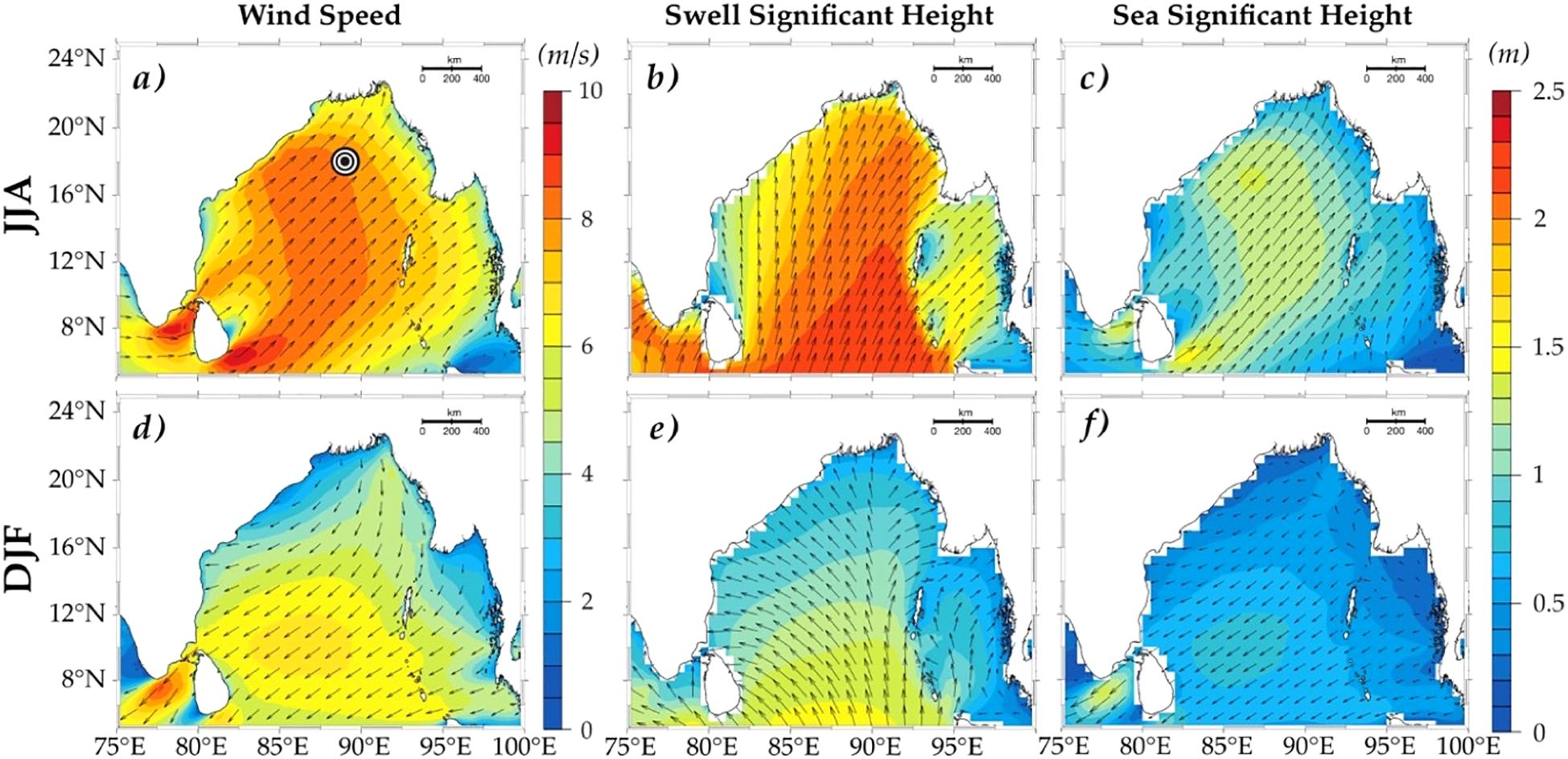
Figure 1. Seasonal averages of (a, d) wind speed (m/s) (shading) and direction (arrows), (b, e) Significant Wave height of Swells (magnitude shading and direction arrows) and (c, f) wind-sea (magnitude shading and direction arrows) during June–August (JJA) and December–February (DJF) from ERA5 data. The Black marker in (a) represents the location of the ECFS mooring at 18°N, 89°E.

The remainder of this paper is organized as follows: Section 2 describes the buoy data used in this study and the correction methods applied. The theoretical background adopted in this study is outlined in Section 3. Section 4 presents the mean sea state conditions prevailing at the buoy location during the data collection period, while Section 5 focuses on the directional analysis of wind stress. Finally, the results are summarized in Section 6.

2 Data and processing methods

The Indian National Centre for Ocean Information Services (INCOIS) deployed a highly instrumented buoy system at 18°N, 89°E in the northern Bay of Bengal (BoB) under the Ocean Mixing and Monsoon (OMM) program. This buoy is equipped with a suite of surface meteorological instruments, including a high-frequency Eddy Covariance Flux System (ECFS) sampling at 20 Hz and a lower-frequency Air-Sea Interaction Meteorology (ASIMET) package operating at 1 Hz. The ECFS setup included a Gill R3-50 sonic anemometer, a LI-7500RS Infrared Gas Analyzer (IRGA), and a Microstrain 3DM-GX5-35 motion sensor pack, all mounted at a height of 3.47 meters above mean sea level. The ECFS data were recorded every hour in 20-minute intervals over 16 months, from May 2019 to August 2020, collecting 12,087 averaged data points.

This study utilized high-frequency data from the sonic anemometer and motion sensors. The measured wind velocities are subject to errors arising from buoy motion. Following Edson et al. (1998) and Fujitani (1981), we applied a motion correction algorithm to remove the influence of platform movement. Corrected wind velocities are then rotated to the mean wind direction using a coordinate rotation procedure (ie; $\overline{v\text{'}}=\overline{w\text{'}}=0$). After removing the linear trend from each 20-min signal, flux was computed as the covariance of horizontal and vertical velocities in the along-wind and cross-wind directions. Using accelerometer and gyroscope data from the motion sensor pack, wave parameters such as significant wave height, peak and mean wave periods, and direction were calculated. Accelerometer data were integrated to obtain velocity and surface elevation, followed by Fast Fourier Transform (FFT)–based spectral analysis to extract wave metrics (Anctil et al., 1993; Thomson et al., 2018). The wind, wave, and associated stress directions used in the study, are defined following the meteorological convention (“from”). Quality control procedures were applied to remove erroneous data caused by instrument errors and outliers, leaving a total of 9,113 valid data points.

We also used the wind speed, significant wave height of wind seas and swells from the ERA-5 reanalysis product, obtained from https://www.ecmwf.int/en/forecasts/dataset/ecmwf-reanalysis-v5, to show the seasonal characteristics in the BoB.

3 Theoretical background

Wind stress vector at levels above the viscous sublayer as measured by eddy covariance methods (e.g., Grachev et al., 2003) may be represented by the following equation:

$\begin{array}{ll}\overrightarrow{\tau }={\tau }_x+{\tau }_y=-\rho \langle u\text{'}w\text{'}\rangle \widehat{i}-\rho \langle v\text{'}w\rangle \widehat{j}& (3)\end{array}$

Where $\langle \rangle$ represents time averaging operator; and $u^{\prime },v^{\prime }and w^{\prime }$ are the longitudinal, lateral, and vertical velocity component fluctuations. Here (in Equation 3), ${\tau }_x=-\rho \langle u\text{'}w\text{'}\rangle \widehat{i}$ is the alongwind component and ${\tau }_y=-\rho \langle v\text{'}w\text{'}\rangle \widehat{J}$ is the cross-wind component of wind stress vector in a coordinate system with x-axis aligned in the mean wind direction. In most studies, stress is assumed to be aligned with the wind direction to ensure that the total τ is predominantly captured by the along-wind stress, rendering the cross-wind component negligible. Standard MOST also assumes this alignment between stress and wind direction and follows $\langle v"w\text{" }\rangle =0$ by definition. However, studies have indicated that these key assumptions of MOST often break down under typical low wind and/or swell conditions and the cross-wind stress component is not always negligible (Geernaert, 1988; Geernaert et al., 1993; Grachev et al., 2003; Chen et al., 2018).

In such a scenario, there will be a deviation of the stress vector from the wind direction (herein after stress-off wind angle, $\text{α}$), which is calculated as (Equation 4);

$\begin{array}{ll}\text{α}=\arctan \left(\frac{\langle v^{\prime }{w}^{\prime }\rangle }{\langle u^{\prime }{w}^{\prime }\rangle }\right)& (4)\end{array}$

Where positive (negative) α corresponds to $\text{τ}$ directed towards the right (left) of the wind vector (Grachev et al., 2003). Studies have shown that at low winds, stress can deviate significantly from the mean wind direction (Drennan et al., 1999; Chen et al., 2018) leaving $\alpha$ exceeding 90° in some cases. This deviation is found to decrease with an increase in wind speed.

Over the ocean, with waves present, the total stress ${\text{τ}}_{\text{total}}$ is the sum of turbulent, wave-induced and viscous components (Phillips, 1977) and ${\text{τ}}_{\text{total}}$ can be expressed as follows:

$\begin{array}{ll}\overrightarrow{{\text{τ}}_{\text{total}}}=\overrightarrow{{\text{τ}}_{\text{turb}}}+\overrightarrow{{\text{τ}}_{\text{wave}}}+\overrightarrow{{\text{τ}}_{\text{visc}}}& (5)\end{array}$

where, $\overrightarrow{{\tau }_{\text{turb}}}$ is the turbulent shear stress, $\overrightarrow{{\tau }_{\text{wave}}}$ is the wave-induced stress responsible for the transfer of momentum to/from the waves, and $\overrightarrow{{\tau }_{\text{visc}}}$ is viscous stress, which is considered negligible, as it is only significant within the millimeter layer just above the sea surface.

The ocean waves span a wide spectrum of frequencies, comprising both locally generated wind waves and remotely generated swells. Swell waves are generated by distant wind systems, meaning their propagation direction remains unaffected by local wind conditions (Alves, 2006; Remya et al., 2020; Sreejith et al., 2022). Locally generated wind waves propagate in the direction of the prevailing winds. In contrast, swells can propagate in directions that do not coincide with the local wind. Hence $\overrightarrow{{\tau }_{\text{wave}}}$ can be approximated by the combined contribution of these two wave systems and Equation 5 is rewritten as;

$\begin{array}{ll}\overrightarrow{{\text{τ}}_{\text{total}}}=\overrightarrow{{\text{τ}}_{\text{turb}}}+\overrightarrow{{\text{τ}}_{\text{wind-sea}}}+\overrightarrow{{\text{τ}}_{\text{swells}}}& (6)\end{array}$

Here, both $\overrightarrow{{\tau }_{\text{turb}}}$ and $\overrightarrow{{\tau }_{\text{wind-sea}}}$ are aligned with the wind direction, while ${\tau }_{\text{swells}}$ follows the direction of swell propagation. Following Grachev et al. (2003), Equation 6 can be further simplified into two components in a coordinate system in the wind direction and the direction of the swell propagation, respectively as; ${\text{τ}}_1=\overrightarrow{{\tau }_{\text{turb}}}+\overrightarrow{{\tau }_{\text{wind-sea}}}$ and ${\text{τ}}_2=\overrightarrow{{\tau }_{\text{swells}}}$. The relationship between this wind-swell coordinate system and the orthogonal coordinate system (as in Equation 3) is illustrated in Figure 2. Here, θ is the angle between the peak wave direction and wind, and α is the stress-off wind angle (Equation 4) and the relationships between these quantities can be represented as:

Figure 2

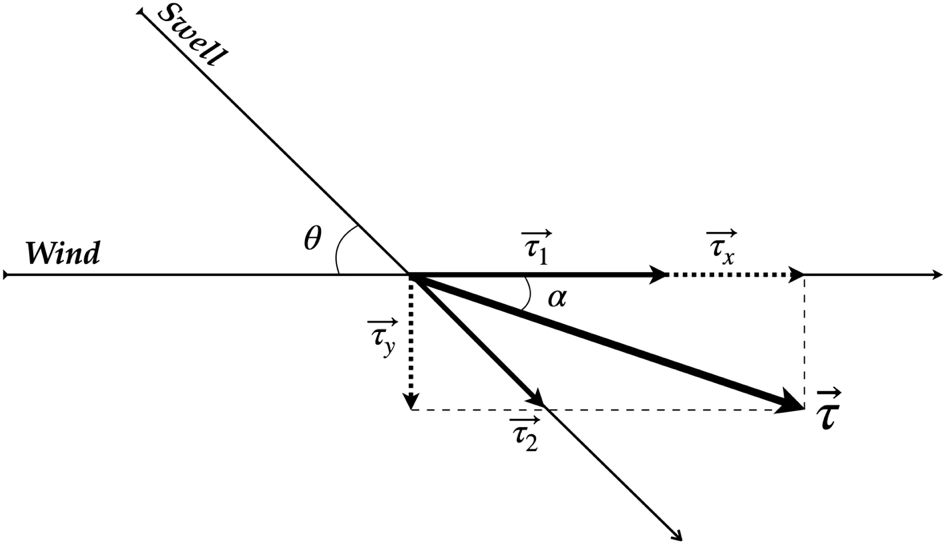
Figure 2. Schematic illustrating the decomposition of stress vector $\tau$, in wind-aligned cartesian coordinates (as ${\tau }_x and {\tau }_y$), and wind-swell coordinates (as ${\tau }_1 and {\tau }_2$). The angle between peak wave direction and wind is θ, and α is the stress-off wind angle.

$\begin{array}{ll}{\text{τ}}_1={\text{τ}}_x-{\text{τ}}_y\cot \theta \hspace{1em}\text{and}\hspace{1em}{\tau }_2=\frac{{\text{τ}}_y}{\sin \text{θ}}& (7)\end{array}$

This decomposition transforms the wind stress from the orthogonal cartesian system to the non-orthogonal wind-swell coordinate system, which is particularly useful in swell-dominated or mixed-seas conditions where swells are prominent. Here, θ or α is taken as positive (negative) if a swell propagation direction or stress vector lies to the right (left) of wind propagation direction. Data corresponds to $\left|\text{θ}\right|\approx$ 0 are discarded as coordinate conversion following Equation 7 fails when $|sin \text{θ}|<0.2$ (Grachev et al., 2003). ${\text{τ}}_1$ and ${\text{τ}}_2$ are positive when aligned with wind and swell directions, respectively. Thus, the total stress ${\text{τ}}_{tot}$ can either be positive or negative, depending on the relative magnitude and direction of ${\text{τ}}_1$ and ${\text{τ}}_2$.

To exlain the sea state characteristics, we used inverse wave age, which is defined as,

$\begin{array}{ll}\text{Inverse Wave Age}=U\cos (\text{θ})/C_p& (8)\end{array}$

Here, $C_p$ is the phase velocity of waves at the spectral peak derived from the peak wave period as $C_p = g T_p/2\pi$, where $T_p$ is the peak wave period, $U$ is the wind speed, and $\theta$ is the angle between wind and wave directions. Wind-wave directional misalignment is taken into consideration by having cosine $\text{θ}$ dependence of wave age (Hanley et al., 2010). A negative inverse wave age thus corresponds to counter swell events, and positive higher values correspond to wind-seas. The definition of sea state based on wave age/inverse wave age still remains a topic of ongoing debate (Li et al., 2024). Rather than endorsing a specific definition, we defined sea state categories based on inverse wave age frequency distribution in our data (Hanley et al., 2010; Patton et al., 2019).

4 Mean sea-state conditions

A notable feature of the BoB’s wind pattern is its seasonal reversal during the monsoon period (Figure 1). As illustrated, the JJA period is marked by prevailing south-westerly winds (Figures 1a, c), which shift to north-easterly during the DJF period (Figures 1d, f). Figure 3a highlights that, during JJA, the wind direction at the buoy location predominantly falls within the 180-270° range, whereas in the DJF period, it is in the 0-90° range. The wave direction at the buoy location ranges from 180-220°, indicating south-westerly waves, except for a few instances during DJF when most swells propagate toward the north-northeast (Figure 3b). These in situ observations align well with the basin-scale wind-wave patterns shown in Figure 1 from ERA-5 data. During JJA, the swell directions are aligned within ±45° of the wind direction. In contrast, both Figure 1 and Figure 3 suggest cross-swell and opposing swell conditions during DJF. Figure 4 presents histograms showing the frequency of occurrence (%) of inverse wave age for JJA and DJF. Here, an inverse wave age value below zero represents the presence of counter-swell conditions, where the swell travels against the wind direction. An inverse wave age greater than 0.8 is considered wind-sea-dominated, where waves grow by absorbing momentum from the local winds. Lower inverse wave ages, less than 0.5, are associated with the old sea and non-locally generated swell and are named swell-dominated conditions. Inverse wave age in the range of 0.5 to 0.8 is considered mixed seas, as it includes both swells, which impart momentum to the wind, and wind seas, which extract momentum from the wind. So, based on this sea state categorization. DJF has more occurrences of counter swells and mixed sea conditions while JJA has swells or mixed sea conditions dominating through the analysis period.

Figure 3

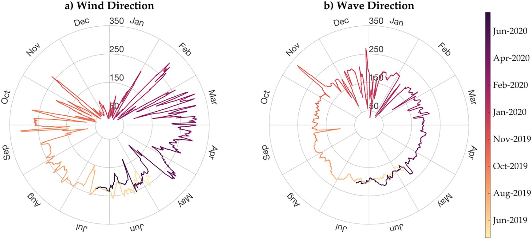
Figure 3. Temporal evolution of wind (a) and wave (b) directions from the Eddy Covariance Flux System (ECFS) mooring at 18°N, 89°E, with direction (in degrees) along radius and months along the perimeter of the circle. Wind and wave directions follows the meteorological convention (“from”).

Figure 4

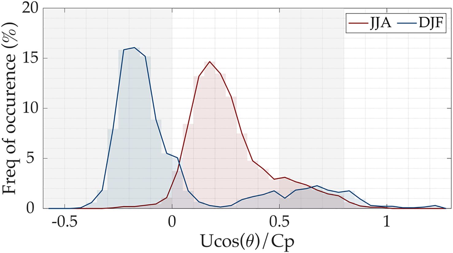
Figure 4. Frequency distribution (%) of inverse wave age ($U\cos (\theta )/C_p$) during June–August (JJA) and December–February (DJF) from the ECFS mooring at 18°N, 89°E.

Figure 5 displays the time series of wind speed (Ws), significant wave height (Hs), inverse wave age (Equation 8), and wind-wave directional alignment angle (θ) data obtained from the buoy deployed at 18°N, 89°E in BoB. Ws ranges from 5 to 13 m/s (Figure 5a), with notable peaks during JJA associated with the Indian summer monsoon. On average, Hs (Figure 5b) reaches ~$4$ meters during the JJA period and decreases to ~$2$ meters during DJF. Clear intra-seasonal oscillations, characteristic of the monsoon, are visible in both Hs and the inverse wave age in JJA. During the active phase of the monsoon, stronger winds lead to a wind-sea-dominated sea state, with Hs increasing and inverse wave age values falling between 0.5 and 0.8 (Figure 5c). This reflects a mixed sea state where wind-sea conditions prevail. In contrast, during the break phase of the monsoon, the sea state transitions to a predominantly swell-dominated regime, with inverse wave age values dropping between 0 and 0.5. In DJF, lower Ws and reduced Hs are observed, resulting in a swell-dominated sea state ($U\cos (\theta )/C_p <0.5$), often transitioning into negative values, indicating counter-swell conditions. The θ (Figure 5d) further highlights that during JJA, swells are aligned at an acute angle to the wind direction, whereas in DJF, a significant portion of the data shows values between 145° and 180°, indicating prevalent counter swell conditions.

Figure 5

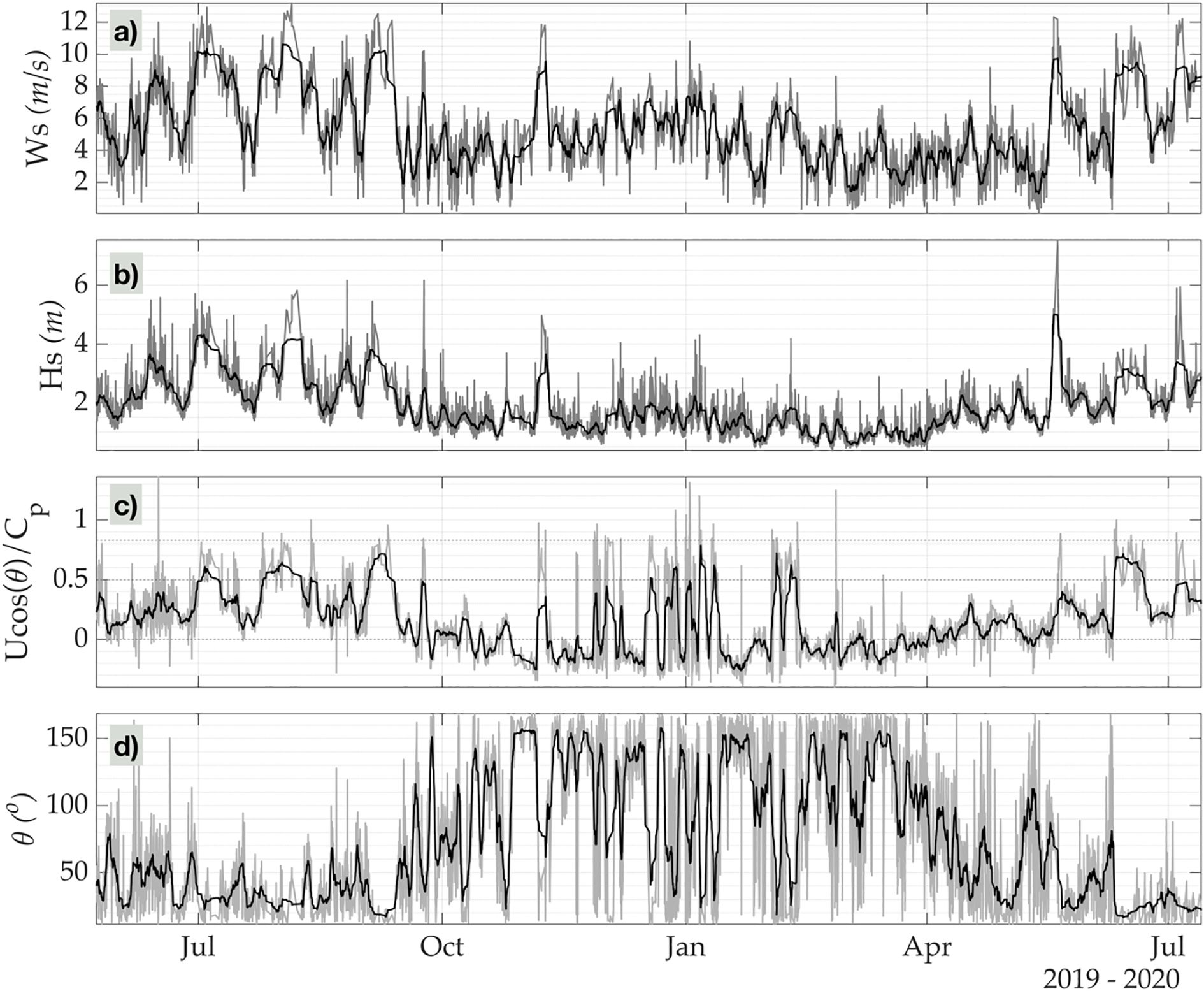
Figure 5. Temporal evolution of (a) Wind speed (m/s), (b) Significant wave height (Hs; m), (c) inverse wave age ($U\cos (\theta )/C_p$), and (d) wind-wave directional alignment angle ($\left|\text{θ}\right|;\text{ deg}$) obtained from the ECFS mooring at 18°N, 89°E. The grey line represents 20-minute averages, and the black line represents daily average values.

5 Directional analysis of wind stress

Figure 6 presents ${\tau }_1$ and ${\tau }_2$ as a function of wind speed for JJA (Figures 6a, b) and DJF (Figures 6c, d). The colour scale indicates the absolute value of the wind-wave angle ($\left|\theta \right|$). ${\tau }_1$ increases with wind speed for both JJA and DJF. On the other hand, ${\tau }_2$ spreads to either side of zero and the scatter increases with wind speed. While both seasons have a similar trend, the increased scatter at higher winds could be attributed to more complex interactions between the local wind sea and swells. Larger $\left|\theta \right|$ suggests a higher amount of misalignment between wind and waves and is seen in DJF.

Figure 6

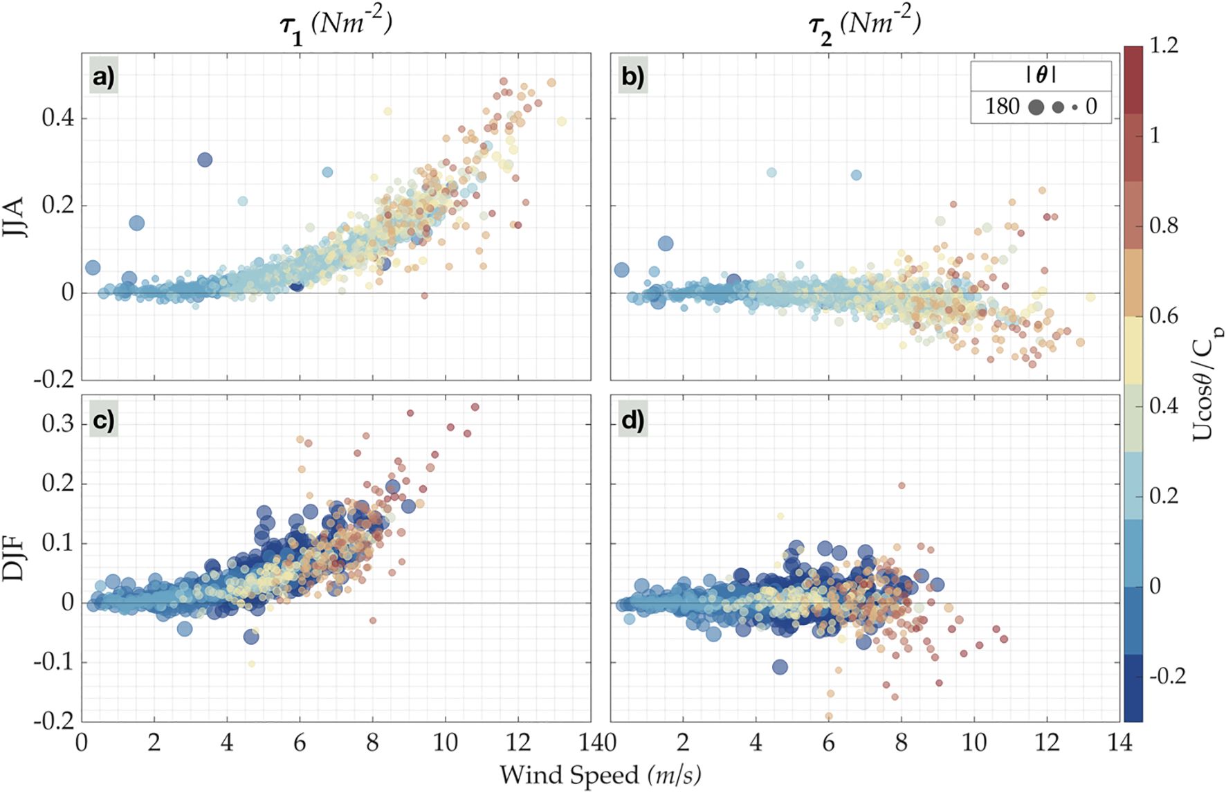
Figure 6. Comparison of wind-aligned (${\text{τ}}_1$) and swell-aligned (${\text{τ}}_2$) stress components (N/m²) against wind speed (m/s) from the ECFS mooring at 18°N, 89°E. (a) ${\text{τ}}_1$ vs wind speed during June-August (JJA), (b) ${\text{τ}}_2$ vs wind speed during JJA, (c) ${\text{τ}}_1$ vs wind speed during December-February (DJF), and (d) ${\text{τ}}_2$ vs wind speed during DJF. Color denotes the inverse wave age ($U\cos (\theta )/C_p$) and marker size shows absolute relative angle between wind and peak-wave directions (|θ|; deg), with larger size representing greater deviation.

Further, we estimated ${\tau }_1$ and ${\tau }_2$ for different possible combinations of θ and α following Equation 7 and defined them as 16 distinct cases. These defined cases, along with their respective conditions and the number of occurrences identified in our study, are summarized in Table 1. During the JJA season, three cases—1, 9 and 11—together account for approximately 90% of the wind stress cases at the study location, which is elaborated further below.

Table 1

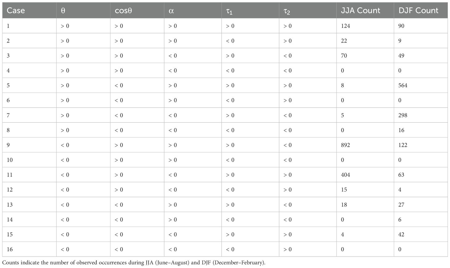
Table 1. Summary of wind-wave alignment conditions. Each represents a unique combination of wind and wave directional alignment condition, as defined in the study.

Case 1 (Figure 7a) occurs when moderate to strong winds blow over swells on the right side of the wind $(\theta > 0,\alpha > 0)$. In this scenario, both ${\tau }_x$ and ${\tau }_y$ are positive, and the stress vector forms an acute angle between the wind and swell propagation directions, lying to the right of the wind vector. As a result, both ${\tau }_1$ and ${\tau }_2$ are positive. This condition contributes ~8% (124 cases) to the total JJA wind stress data.

Figure 7

Figure 7. Schematic diagrams of the five most frequent wind-swell-stress interaction cases observed during June-August (JJA) and December-February (DJF) in the Bay of Bengal. (a) Case 1 (JJA: 124; DJF: 90): Moderate-strong winds with swells to the wind’s right. (b) Case 9 (JJA: 892; DJF: 122): Weak winds and near-aligned stronger swells. (c) Case 11 (JJA: 404; DJF: 63): Moderate-strong winds with swells to the wind’s left. (d) Case 5 (JJA: 8; DJF: 564): Strong counter-swells opposing weak-moderate winds. (e) Case 7 (JJA: 5; DJF: 298): Strong winds opposing weaker swells. The number of occurrences for each season are given in parentheses.

Case 11 (Figure 7c), which makes up ~26% (404 cases) of the JJA data, occurs when strong winds blow over swells to the left of the wind $(\theta <0,\alpha <0)$. Similar to Case 1, both ${\tau }_1$ and ${\tau }_2$ are positive, and the total stress vector lies at an acute angle between the wind and swell directions. Cases 1 and 11 represent scenarios with strong winds over swells, together contributing ~34% of JJA data, with the primary difference being the swell orientation—to the right of the wind in Case 1 and to the left in Case 11. Since the wind and swell move in the similar direction and the winds are stronger, the strongly coupled wind waves can still grow and extract momentum from the wind. These wind waves co-exist with (ride) swells. Since $\text{τ}$ lies in the acute angle between wind and swell, the sea state due to swell might play a more important role. That is, for a given wind speed, the aligned swell results in a lower roughness making ${\tau }_1<{\tau }_x$.

As wind speed decreases or the swells strengthen, the swell-induced ${\tau }_2$ reverses sign, leading to Case 9 (Figure 7b). Here the swells act as a drag on the airflow above. This situation is the most common during our observation periods which occurs for 57% (892 cases) of JJA period. In Case 9, weak to moderate winds blow over strong swells. Here, the swell moves faster than the wind, resulting in a different $\tau$ vector alignment. This can be either swells in the direction of wind or cross-wind. This case is characterized byxxx $\text{θ}\langle 0\hspace{0.33em}\text{and}\hspace{0.33em}\alpha \rangle 0$, with the $\tau$ vector positioned to the right of the wind vector, forming an obtuse angle between the wind direction and the direction opposite to swell propagation. In this scenario, ${\tau }_x$, ${\tau }_y$, and ${\tau }_1$ are positive, while ${\tau }_2$ is negative, pointing opposite to the swell propagation (Figure 7b). The negative swell-induced stress under this case results in $\tau$ to orient between wind and opposite swell direction. Theoretically, when weak winds exist over strong aligned swells, the net stress can become negative, and a momentum transfer happens from waves to wind [Observation: Grachev and Fairall (2001), LES: Sullivan et al. (2008), Numerical model: Kudryavtsev and Makin (2004)]. Cross-wind stress component can be non negligible if $\left|\text{θ}\right|$ increases. In short, in the northern BoB, during the JJA season, the swell is predominantly unidirectional, moving from south to north, while wind direction (Figure 3) and magnitude vary particularly on intraseasonal time-scales (Figure 5a). The transitions between cases 1, 9, and 11 are primarily driven by wind speed and direction changes.

During the DJF, the wind stress was predominantly contributed by cases 5, 7, and 9, which together accounted for 76% (984 cases) of the entire season. Of these, approximately 9% corresponded to case 9, characterized by strong background swells combined with weak to moderate winds—a scenario similar to that discussed for JJA. Unlike JJA, where most data indicated nearly aligned wind and wave conditions, DJF saw about 67% (862 cases) of the cases involving counter swells $(\text{θ}>0\hspace{0.33em}\text{and}\hspace{0.33em}\cos \text{θ}<0)$ represented by cases 5 and 7 in Table 1.

Case 5 (Figure 7d) shows counter-swell conditions, where strong swells coexist with weak to moderate winds. $\tau$ is aligned in the direction between swells and wind, with stress magnitude found to be amplified by the counter swells, as discussed by Husain et al. (2022). Observational and large-eddy simulation (LES) studies indicate that swells influence boundary-layer vortical structures, either amplifying or dampening near-surface turbulence based on the alignment of wind and swell directions and wave age. For instance, LES findings reveal increased stress when strong opposing swells induce wave-coherent motions, altering near-surface shear (Sullivan et al., 2008). In this case, the swell-induced stress component is positive $({\tau }_2> 0)$. However, as the wind gets stronger, and/or swells weakens ${\tau }_2$ decreases and becomes negative, as observed in case 7 (Figure 7e). This scenario is marked by dominant, steady winds over relatively weak, opposing waves, with $\tau$ aligning at an acute angle between the wind and the opposing swell direction.

Figure 8 presents the scatter diagram of ${\text{τ}}_1$ vs ${\text{τ}}_x$ for both JJA and DJF. The most occurring cases namely 1, 9, and 11 for JJA (Figure 8a) and 9, 5 and 7 for DJF (Figure 8b) are highlighted with different colours. The grey-shaded region shows the distribution of ${\text{τ}}_1$ vs ${\text{τ}}_x$ from all other cases. A linear relationship is observed, where ${\text{τ}}_x$ increases as ${\text{τ}}_1$ increases. In both seasons, for Case 9 (blue colour), ${\text{τ}}_1$ is higher in magnitude compared to ${\text{τ}}_x$. This condition corresponds to a swell-dominated regime with wind-following swell. In contrast, Cases 11 and 1 in JJA, characterized by moderate to strong winds with light swell aligned to the wind, show ${\text{τ}}_1< {\text{τ}}_x$ with the difference between them increasing as the magnitude of wind stress rises.

Figure 8

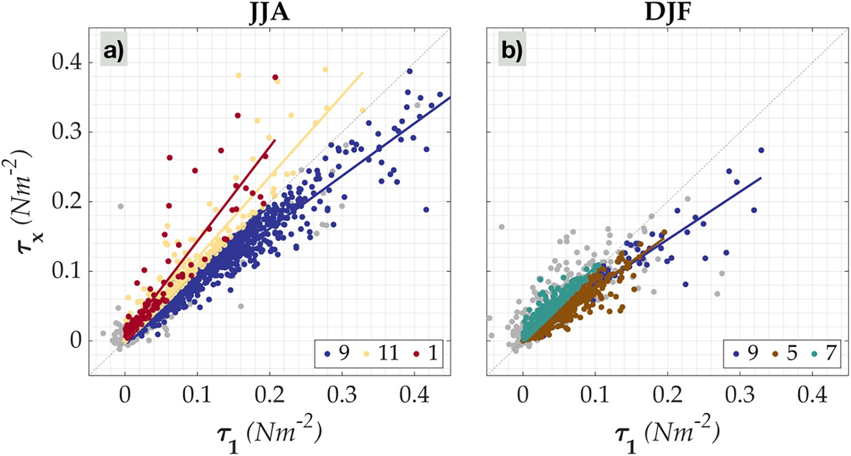
Figure 8. Scatter diagram of wind-aligned stress component in non-orthogonal (wind-swell) coordinates (${\tau }_1$) and orthogonal (cartesian) coordinates (${\tau }_x$) for for (a) June-August (JJA) and (b) December-February (DJF) from the ECFS mooring. Grey shading represents all cases, while color-coded points highlight the most frequent cases: Case 9 (blue), Case 11 (yellow), Case 1 (red), Case 5 (brown), and Case 7 (teal). The dotted 1:1 line indicates perfect agreement (${\text{τ}}_1={\text{τ}}_x$) and colored lines show case-specific linear fits.

Cases 5, 7, 8, 13, 14, and 15 from Table 1 correspond to counter-swell conditions. Under case 7 (Figure 8b), ${\text{τ}}_1$ is having comparable magnitude as ${\text{τ}}_x$, representing situations where strong winds oppose the swell. Conversely, in case 5, where swells dominate, ${\text{τ}}_1$ tends to be larger than ${\text{τ}}_x$. Counter swells tend to increase surface friction compared to wind-following waves (Husain et al., 2022), leading to higher wind stress and drag, particularly at low wind speeds and strong counter swells (García-Nava et al., 2009). However, at higher wind speeds, the presence of swell can reduce drag by modifying surface roughness. These dynamics demonstrate that wind stress critically depends on the combined effects of wind-swell alignment and their relative magnitudes.

To investigate this relationship further, the percentage contribution of stress from various sea state categories, classified based on inverse wave age as described in Section 4 is presented in Figure 9. The percentage contributions of different sea state categories to stress during JJA and DJF are determined for wind speed intervals of 1 m/s.

Figure 9

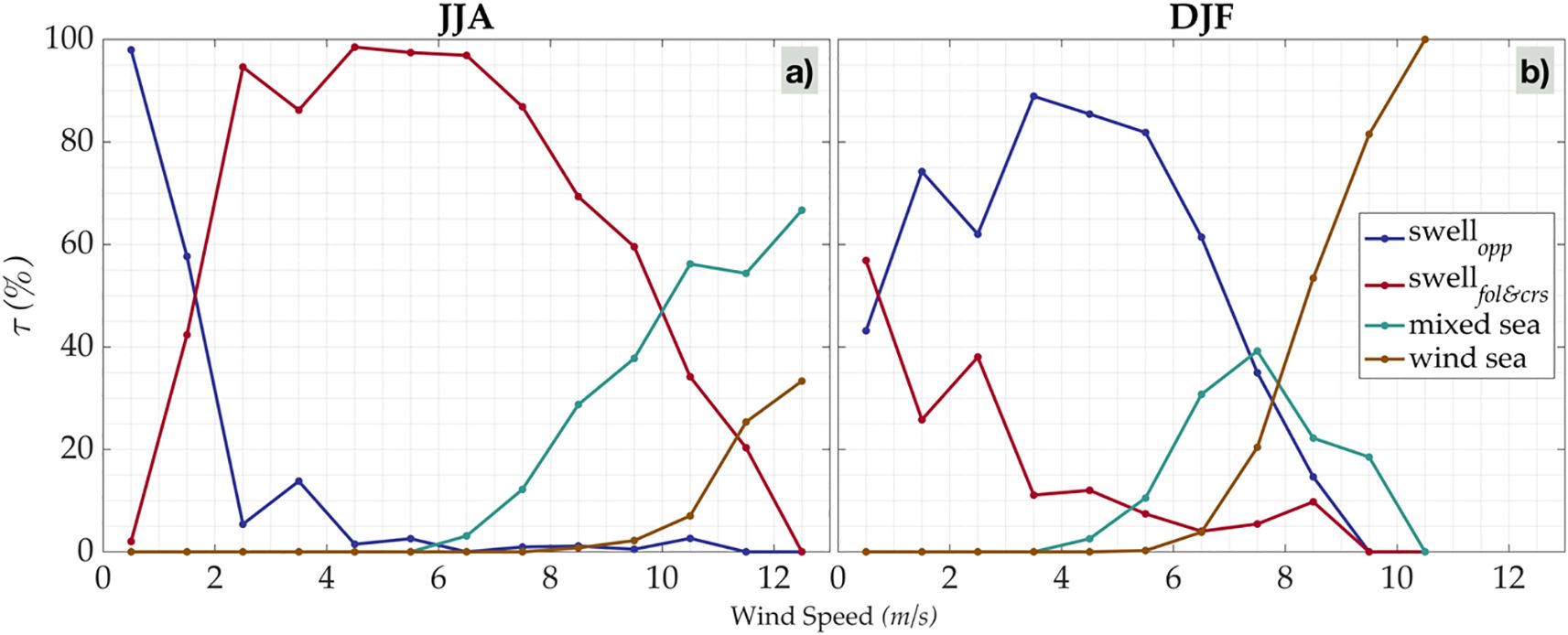
Figure 9. Contribution of sea state categories to along-wind stress (${\tau }_x$) across wind speeds (grouped into 1 m s_-¹ bins) for (a) June-August (JJA) and (b) December-February (DJF) from the ECFS mooring. Sea states are classified by inverse wave age ($U\cos (\theta )/C_p$) and color-coded as: Counter swells (blue) when ($U\cos (\theta )/C_p$)<0, Swell-dominated (red) when 0<($U\cos (\theta )/C_p$)<0.5 indicates old sea and non-locally generated swell, Mixed seas (green) when 0.5<($U\cos (\theta )/C_p$)<0.8 and Wind-sea dominated (brown) when ($U\cos (\theta )/C_p$)> 0.8.

In JJA (Figure 9a), under low wind conditions, surface stress is mainly driven by swells. At wind speeds below 2 m/s, counter swells contribute the majority (~90%) of the stress, with the remainder supported by along and cross swells. As wind speed increases, the contribution from counter swells decreases, while that of along and cross swells rises to approximately 80%. The influence of wind sea becomes evident as wind speed increases, but mixed seas dominate through JJA under this wind regime. In DJF (Figure 9b), under low to moderate wind conditions, counter swells remain the primary contributors to surface stress, with along and cross swells providing the rest. As wind speeds increase, the contribution of the wind sea becomes more significant. Mixed sea contributions appear at wind speeds above 5 m/s and gradually decline as wind sea-induced stress becomes dominant. Over most of the wind speed range observed in the BoB, the contribution of swell to stress is striking. These swells, being decoupled from local winds, pose challenges to MOST-based bulk flux parameterizations, which mostly rely on wind-speed-dependent roughness lengths and transfer coefficients. Such formulations often fail to capture the true magnitude of τ, particularly in swell-dominated conditions.

In order to check that, we compared the COARE 3.6-derived bulk momentum flux against direct EC flux measurements. COARE 3.6 provides two formulations for the calculation of the roughness length, the Wind-Based Formulation (WiBF) and Wave-Based Formulation (WBF), based on field observations (Blomquist et al., 2017; Brumer et al., 2017b, 2017a). Figure 10 shows the percentage bias in stress from these two estimates across sea states categorized by inverse wave age. The results show significant underestimations by both WiBF and WBF under swell-influenced conditions. In counter-swell conditions, the underestimations were 9.4% (WiBF) and 15.5% (WBF) while in aligned swell dominated conditions, the underestimations were 5.2% (WiBF) and 10.1% (WBF). Deviations were smaller in mixed sea states with WiBF showing modest underestimation (4.2%), while WBF exhibited a 6.7% overestimation. For wind sea dominated regime, WiBF performs well with marginal bias (~2.8%). Overall, WBF exhibited greater bias than WiBF in both swell-dominated and wind-sea-dominated conditions, suggesting that the incorporation of sea-state information in its current form does not improve and may even degrade the accuracy of momentum flux estimates compared to the purely wind-based WiBF approach.

Figure 10

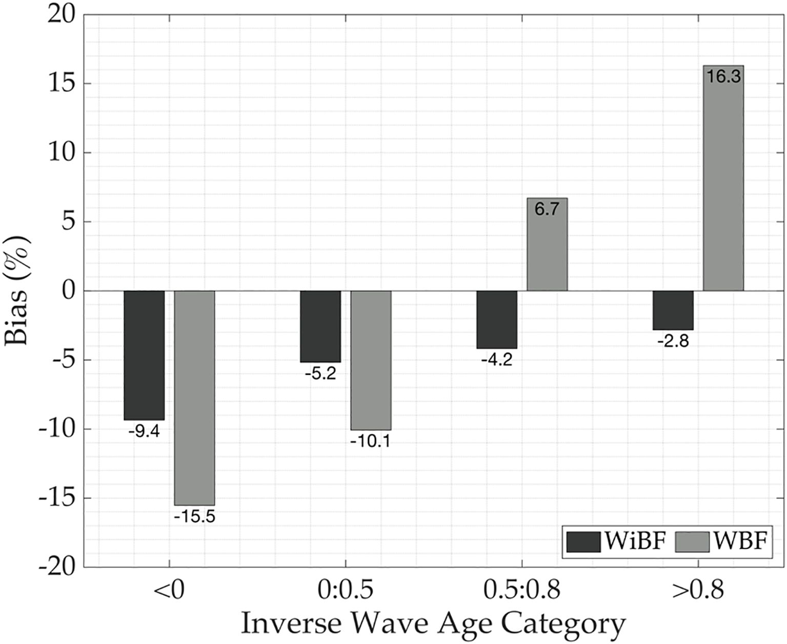
Figure 10. Percentage bias in momentum flux ($\text{τ}$) estimates from the COARE 3.6 bulk model, comparing the Wind-based Formulation (WiBF) and the Sea-state-based Formulation (WBF) against eddy covariance (EC) measurements at the ECFS mooring site. Results are categorized by sea state, with classifications (based on inverse wave age) as defined in Figure 9.

MOST-based bulk flux formulations estimate only the along-wind wind stress. But, cross swells add a non-zero cross-wind component to stress and can result in enhanced stress estimates. Hence the observed deviations are primarily driven by the inability of such bulk flux formulations to account for wind-swell misalignment appropriately in swell-dominated sea state conditions, and the resulting swell-induced stress component. Strong Counter swells result in an enhanced stress transfer due to additional drag. These influences are not negligible and necessitate the inclusion of wind-swell interactions in bulk flux parameterizations to improve their accuracy, as evidenced by Figure 10. The findings underscore the need for better accounting the sea state dynamics in momentum flux estimation, especially in regions where swells dominate and/or low wind conditions.

6 Summary and discussions

The present study investigates wind stress vector directionality under various wind-wave conditions using 16-month-long high-frequency eddy covariance flux and wave data from a moored buoy in the Bay of Bengal (BoB). By decomposing the wind stress vector into components aligned with the wind (${\tau }_1$) and swell directions (${\tau }_2$), following the method of Grachev et al. (2003), we explored how the stress vector orientation varies relative to wind and swell directions and their respective magnitudes. Our findings underscore the significant influence of swells on momentum transfer, particularly under swell-dominated conditions where the stress vector deviates from the mean wind direction.

The BoB’s seasonally reversing monsoonal winds present diverse wind-swell alignment scenarios. During JJA, winds and swells are mostly aligned, while counter-swells dominate DJF. When winds are stronger and aligned with swells during JJA, the stress vector orients between wind and swell directions, contributing to ~34% of cases (528 observations). In these situations, young or developing seas extract momentum from the wind, leading to a net reduction in along-wind stress magnitude (${\tau }_1$ < ${\tau }_x$). Conversely, as aligned/cross swells strengthen or wind speeds decrease, the swell-induced stress component (${\tau }_2$) reverses direction towards the swell, increasing the along wind stress magnitude (${\tau }_1$ > ${\tau }_x$). Most JJA cases fall into this category (57%), with the stress vector oriented between wind and opposing swell directions. In DJF, counter swells, when combined with weak to moderate winds result in increased along-wind stress magnitudes (${\tau }_1$ > ${\tau }_x$). The stress vector aligns between the wind and opposing swell direction, consistent with findings by Husain et al. (2022). Counter-swell conditions substantially increase surface friction compared to aligned swell or wind-sea states, highlighting the role of wind-swell directional misalignment in modifying stress dynamics. In DJF, the combined effects of counter swells and moderate winds similarly amplify stress challenging the assumptions of constant flux layers and steady-state dynamics inherent in MOST. Studies like Chen et al. (2019) have further shown that swell-induced influences can extend up to 26m above the sea surface, reinforcing the limitations of conventional parameterizations.

Further analysis of stress component contributions to the total wind stress across different sea state categories confirms the swell-induced stress dominance under low wind conditions across seasons. As previously discussed, these swells, often decoupled from local winds, pose challenges to bulk flux parameterizations based on Monin-Obukhov Similarity Theory (MOST). To evaluate this, we applied the COARE 3.6 algorithm, which includes two options for estimating roughness length: a wind-speed-based formulation (WiBF) and a wave-based formulation (WBF). Comparisons of COARE 3.6-derived bulk momentum fluxes from WiBF and WBF against EC measurements reveal significant discrepancies under swell-influenced conditions. In counter-swell scenarios, COARE underestimates momentum flux by approximately 12% (9.4% in case of WiBF and 15.5% in case of WBF), while in aligned swell conditions, the underestimations are less ~7% (5.2% and 10.1%, respectively for WiBF and WBF). In both cases, the percentage of bias is more than the targeted uncertainty of <5% (Cronin et al., 2019). In contrast, under mixed or wind-sea-dominated states, WiBF estimates show only marginal deviations from EC observations, indicating better agreement. Overall, WBF exhibits a larger bias than WiBF under both swell- and wind-sea-dominated regimes, suggesting that the current formulation of sea-state based parameterization for the roughness length calculation reduce the accuracy of momentum flux estimates. These results underscore the need to better account the wind-swell misalignment and swell-induced stress components in bulk flux formulations, particularly in low-wind, swell-dominated environments.

The in-situ bulk momentum flux data typically used for model validation are derived from moorings or ships employing marine meteorological data forced with a bulk flux model. However, as demonstrated in this study, the magnitude of τ is often underestimated in low-wind and/or swell-dominated conditions. In such cases, the in-situ τ data itself becomes an imperfect reference, potentially leading to misleading validation results for model simulations. This underscores the critical influence of wind-swell directional misalignment on the accuracy of bulk flux-derived τ and highlights the necessity of incorporating more accurate sea-state dynamics into flux parameterizations for accurate validation.

Previous studies on air-sea momentum transfer have been constrained by limited data periods and/or region specificity in their findings. Using long-term data from a mooring in the northern BoB, this study advances our understanding of wind stress directionality by providing detailed insights into stress dynamics in a seasonally wind-reversing, swell-dominated basin. This study also notes that the wind-wave alignment angle and the relative strength of winds and swells influence the magnitude and direction of the wind stress vector – processes that work consistently across diverse oceanic regimes, independent of geographic location. These findings have implications for improving air-sea interaction models by better integrating and representing sea-state information into wind stress parameterizations. While such formulations already exist, further research is needed to refine and validate them across diverse oceanic regimes before incorporating them into coupled climate models.

Data availability statement

The ERA5 reanalysis data are obtained from “https://cds.climate.copernicus.eu/datasets/reanalysis-era5-single-levels?tab=overview”. Version 3.6 of the COARE bulk flux algorithm is available at “https://github.com/NOAA-PSL/COARE-algorithm”. Further inquiries can be directed to the corresponding author.

Author contributions

AR: Investigation, Methodology, Writing – review & editing, Conceptualization, Data curation, Formal Analysis, Software, Visualization, Writing – original draft. BK: Conceptualization, Investigation, Methodology, Writing – review & editing, Funding acquisition, Project administration, Resources, Supervision, Validation. VJ: Formal Analysis, Investigation, Writing – review & editing. PR: Formal Analysis, Investigation, Writing – review & editing. HS: Formal Analysis, Investigation, Writing – review & editing. NS: Formal Analysis, Investigation, Writing – review & editing. EP: Formal Analysis, Investigation, Writing – review & editing.

Funding

The author(s) declare financial support was received for the research and/or publication of this article. Ministry of Earth Sciences (MoES), Govt. of India provided the necessary funding to carry out this research.

Acknowledgments

The EC data used in this study comes from the Bay of Bengal mooring deployed as part of the Ministry of Earth Sciences (MoES, Govt. of India) funded Monsoon Mission project, ‘Coupled Physical Processes in the Bay of Bengal and Monsoon Air-Sea Interaction (Ocean Mixing and Monsoon)’. The crew of ORV Sagar Nidhi who deployed and recovered the mooring, is especially thanked for their service. This article is part of AR’s doctoral research, and he acknowledges the research fellowship through the Ministry of Earth Sciences (MoES, Govt. of India) “Development of Skilled Manpower in Earth Sciences (DESK)” Program. HS acknowledges the support from the U.S. Office of Naval Research (N00014-24-1-2570). This article has INCOIS contribution number 585.

Conflict of interest

The authors declare that the research was conducted in the absence of any commercial or financial relationships that could be construed as a potential conflict of interest.

Generative AI statement

The author(s) declare that no Generative AI was used in the creation of this manuscript.

Any alternative text (alt text) provided alongside figures in this article has been generated by Frontiers with the support of artificial intelligence and reasonable efforts have been made to ensure accuracy, including review by the authors wherever possible. If you identify any issues, please contact us.

Publisher’s note

All claims expressed in this article are solely those of the authors and do not necessarily represent those of their affiliated organizations, or those of the publisher, the editors and the reviewers. Any product that may be evaluated in this article, or claim that may be made by its manufacturer, is not guaranteed or endorsed by the publisher.

References

Alves J.-H. G. M. (2006). Numerical modeling of ocean swell contributions to the global wind-wave climate. Ocean Model. 11, 98–122. doi: 10.1016/j.ocemod.2004.11.007

Crossref Full Text | Google Scholar

Anctil F., Donelan M. A., Forristall G. Z., Steele K. E., and Ouellet Y. (1993). Deep-water field evaluation of the NDBC-SWADE 3-m discus directional buoy. J. Atmos Oceanic Tech 10, 97. doi: 10.1175/1520-0426(1993)010<0097:DWFEOT>2.0.CO;2

Crossref Full Text | Google Scholar

Blomquist B. W., Brumer S. E., Fairall C. W., Huebert B. J., Zappa C. J., Brooks I. M., et al. (2017). Wind speed and sea state dependencies of air-sea gas transfer: results from the high wind speed gas exchange study (HiWinGS). JGR Oceans 122, 8034–8062. doi: 10.1002/2017JC013181

Crossref Full Text | Google Scholar

Brumer S. E., Zappa C. J., Blomquist B. W., Fairall C. W., Cifuentes-Lorenzen A., Edson J. B., et al. (2017a). Wave-related reynolds number parameterizations of CO₂ and DMS transfer velocities. Geophysical Res. Lett. 44, 9865–9875. doi: 10.1002/2017GL074979

Crossref Full Text | Google Scholar

Brumer S. E., Zappa C. J., Brooks I. M., Tamura H., Brown S. M., Blomquist B. W., et al. (2017b). Whitecap coverage dependence on wind and wave statistics as observed during SO gasEx and hiWinGS. J. Phys. Oceanography 47, 2211–2235. doi: 10.1175/JPO-D-17-0005.1

Crossref Full Text | Google Scholar

Chen S., Qiao F., Huang C. J., and Zhao B. (2018). Deviation of wind stress from wind direction under low wind conditions. JGR Oceans 123, 9357–9368. doi: 10.1029/2018JC014137

Crossref Full Text | Google Scholar

Chen S., Qiao F., Jiang W., Guo J., and Dai D. (2019). Impact of surface waves on wind stress under low to moderate wind conditions. J. Phys. Oceanography 49, 2017–2028. doi: 10.1175/JPO-D-18-0266.1

Crossref Full Text | Google Scholar

Chen S., Qiao F., Xue Y., Chen S., and Ma H. (2020). Directional characteristic of wind stress vector under swell-dominated conditions. JGR Oceans 125, e2020JC016352. doi: 10.1029/2020JC016352

Crossref Full Text | Google Scholar

Cronin M. F., Gentemann C. L., Edson J., Ueki I., Bourassa M., Brown S., et al. (2019). Air-sea fluxes with a focus on heat and momentum. Front. Mar. Sci. 6. doi: 10.3389/fmars.2019.00430

Crossref Full Text | Google Scholar

Donelan M. A., Dobson F. W., Smith S. D., and Anderson R. J. (1993). On the dependence of sea surface roughness on wave development. J. Phys. Oceanogr. 23, 2143–2149. doi: 10.1175/1520-0485(1993)023<2143:OTDOSS>2.0.CO;2

Crossref Full Text | Google Scholar

Drennan W. M. (2003). On the wave age dependence of wind stress over pure wind seas. J. Geophys. Res. 108, 8062. doi: 10.1029/2000JC000715

Crossref Full Text | Google Scholar

Drennan W. M., Kahma K. K., and Donelan M. A. (1999). On momentum flux and velocity spectra over waves. Boundary-Layer Meteorology 92, 489–515. doi: 10.1023/A:1002054820455

Crossref Full Text | Google Scholar

Drennan W. M., Taylor P. K., and Yelland M. J. (2005). Parameterizing the sea surface roughness. J. Phys. Oceanography 35, 835–848. doi: 10.1175/JPO2704.1

Crossref Full Text | Google Scholar

Edson J. B., Hinton A. A., Prada K. E., Hare J. E., and Fairall C. W. (1998). Direct covariance flux estimates from mobile platforms at sea*. J. Atmos. Oceanic Technol. 15, 547–562. doi: 10.1175/1520-0426(1998)015<0547:DCFEFM>2.0.CO;2

Crossref Full Text | Google Scholar

Edson J. B., Jampana V., Weller R. A., Bigorre S. P., Plueddemann A. J., Fairall C. W., et al. (2013). On the exchange of momentum over the open ocean. J. Phys. Oceanography 43, 1589–1610. doi: 10.1175/JPO-D-12-0173.1

Crossref Full Text | Google Scholar

Fairall C. W., Bradley E. F., Rogers D. P., Edson J. B., and Young G. S. (1996). Bulk parameterization of air-sea fluxes for Tropical Ocean-Global Atmosphere Coupled-Ocean Atmosphere Response Experiment. J. Geophys. Res. 101, 3747–3764. doi: 10.1029/95JC03205

Crossref Full Text | Google Scholar

Foken T. (2006). 50 years of the monin–obukhov similarity theory. Boundary-Layer Meteorol 119, 431–447. doi: 10.1007/s10546-006-9048-6

Crossref Full Text | Google Scholar

Fujitani T. (1981). Direct measurement of turbulent fluxes over the sea during AMTEX. Pap. Met. Geophys. 32, 119–134. doi: 10.2467/mripapers.32.119

Crossref Full Text | Google Scholar

García-Nava H., Ocampo-Torres F. J., Osuna P., and Donelan M. A. (2009). Wind stress in the presence of swell under moderate to strong wind conditions. J. Geophys. Res. 114, C12008. doi: 10.1029/2009JC005389

Crossref Full Text | Google Scholar

Geernaert G. L. (1988). Measurements of the angle between the wind vector and wind stress vector in the surface layer over the North Sea. J. Geophys. Res. 93, 8215–8220. doi: 10.1029/JC093iC07p08215

Crossref Full Text | Google Scholar

Geernaert G. L., Hansen F., Courtney M., and Herbers T. (1993). Directional attributes of the ocean surface wind stress vector. J. Geophys. Res. 98, 16571–16582. doi: 10.1029/93JC01439

Crossref Full Text | Google Scholar

Grachev A. A. and Fairall C. W. (2001). Upward momentum transfer in the marine boundary layer. J. Phys. Oceanogr. 31, 1698–1711. doi: 10.1175/1520-0485(2001)031<1698:UMTITM>2.0.CO;2

Crossref Full Text | Google Scholar

Grachev A. A., Fairall C. W., Hare J. E., Edson J. B., and Miller S. D. (2003). Wind stress vector over ocean waves. J. Phys. Oceanogr. 33, 2408–2429. doi: 10.1175/1520-0485(2003)033<2408:WSVOOW>2.0.CO;2

Crossref Full Text | Google Scholar

Hanley K. E. and Belcher S. E. (2008). Wave-driven wind jets in the marine atmospheric boundary layer. J. Atmospheric Sci. 65, 2646–2660. doi: 10.1175/2007JAS2562.1

Crossref Full Text | Google Scholar

Hanley K. E., Belcher S. E., and Sullivan P. P. (2010). A global climatology of wind–wave interaction. J. Phys. Oceanography 40, 1263–1282. doi: 10.1175/2010JPO4377.1

Crossref Full Text | Google Scholar

Hara T. and Sullivan P. P. (2015). Wave boundary layer turbulence over surface waves in a strongly forced condition. J. Phys. Oceanography 45, 868–883. doi: 10.1175/JPO-D-14-0116.1

Crossref Full Text | Google Scholar

Husain N. T., Hara T., and Sullivan P. P. (2022). Wind turbulence over misaligned surface waves and air–sea momentum flux. Part I: waves following and opposing wind. J. Phys. Oceanography 52, 119–139. doi: 10.1175/JPO-D-21-0043.1

Crossref Full Text | Google Scholar

Kahma K. K., Donelan M. A., Drennan W. M., and Terray E. A. (2016). Evidence of energy and momentum flux from swell to wind. J. Phys. Oceanography 46, 2143–2156. doi: 10.1175/JPO-D-15-0213.1

Crossref Full Text | Google Scholar

Kudryavtsev V. N. and Makin V. K. (2004). Impact of swell on the marine atmospheric boundary layer. J. Phys. Oceanogr. 34, 934–949. doi: 10.1175/1520-0485(2004)034<0934:IOSOTM>2.0.CO;2

Crossref Full Text | Google Scholar

Large W. G. and Pond S. (1981). Open ocean momentum flux measurements in moderate to strong winds. J. Phys. Oceanogr. 11, 324–336. doi: 10.1175/1520-0485(1981)011<0324:OOMFMI>2.0.CO;2

Crossref Full Text | Google Scholar

Li S. (2023). On the consistent parametric description of the wave age dependence of the sea surface roughness. J. Phys. Oceanography 53, 2281–2290. doi: 10.1175/JPO-D-23-0021.1

Crossref Full Text | Google Scholar

Li H., Chapron B., Vandemark D., Lin W., Hauser D., He Y., et al. (2024). A novel sea state classification scheme of the global CFOSAT wind and wave observations. JGR Oceans 129, e2023JC020686. doi: 10.1029/2023JC020686

Crossref Full Text | Google Scholar

Monin A. S. and Obukhov A. M. (1954). Basic laws of turbulent mixing in the surface layer of the atmosphere. Geophys. Inst. Acad. Sci. USSR 24, -163–-187.

Google Scholar

Oost W. A., Komen G. J., Jacobs C. M. J., and Van Oort C. (2002). New evidence for a relation between wind stress and wave age from measurements during ASGAMAGE. Boundary-Layer Meteorology 103, 409–438. doi: 10.1023/A:1014913624535

Crossref Full Text | Google Scholar

Patton E. G., Sullivan P. P., Kosović B., Dudhia J., Mahrt L., Žagar M., et al. (2019). On the influence of swell propagation angle on surface drag. J. Appl. Meteorology Climatology 58, 1039–1059. doi: 10.1175/JAMC-D-18-0211.1

Crossref Full Text | Google Scholar

Phillips O. M. (1997). The Dynamics of the upper ocean. 2nd ed (Cambridge: Cambridge University Press).

Google Scholar

Raj A., Praveen Kumar B., Jampana V., Shivaprasad S., Sureshkumar N., Rao E. P. R., et al. (2024). Turbulent characteristics of momentum flux in the marine atmospheric boundary layer of North Bay of Bengal. Sci. Rep. 14, 22073. doi: 10.1038/s41598-024-71819-z

PubMed Abstract | Crossref Full Text | Google Scholar

Reichl B. G., Hara T., and Ginis I. (2014). Sea state dependence of the wind stress over the ocean under hurricane winds. JGR Oceans 119, 30–51. doi: 10.1002/2013JC009289

Crossref Full Text | Google Scholar

Remya P. G., Kumar B. P., Srinivas G., and Nair T. M. B. (2020). Impact of tropical and extra tropical climate variability on Indian Ocean surface waves. Clim Dyn 54, 4919–4933. doi: 10.1007/s00382-020-05262-x

Crossref Full Text | Google Scholar

Sauvage C., Seo H., Barr B. W., Edson J. B., and Clayson C. A. (2024). Misaligned wind-waves behind atmospheric cold fronts. JGR Oceans 129, e2024JC021162. doi: 10.1029/2024JC021162

Crossref Full Text | Google Scholar

Sauvage C., Seo H., Clayson C. A., and Edson J. B. (2023). Improving wave-based air-sea momentum flux parameterization in mixed seas. JGR Oceans 128, e2022JC019277. doi: 10.1029/2022JC019277

Crossref Full Text | Google Scholar

Semedo A., Sušelj K., Rutgersson A., and Sterl A. (2011). A global view on the wind sea and swell climate and variability from ERA-40. J. Climate 24, 1461–1479. doi: 10.1175/2010JCLI3718.1

Crossref Full Text | Google Scholar

Sreejith M., P. G. R., Kumar B. P., Raj A., and Nair T. M. B. (2022). Exploring the impact of southern ocean sea ice on the Indian Ocean swells. Sci. Rep. 12, 12360. doi: 10.1038/s41598-022-16634-0

PubMed Abstract | Crossref Full Text | Google Scholar

Sullivan P. P., Edson J. B., Hristov T., and McWilliams J. C. (2008). Large-eddy simulations and observations of atmospheric marine boundary layers above nonequilibrium surface waves. J. Atmospheric Sci. 65, 1225–1245. doi: 10.1175/2007JAS2427.1

Crossref Full Text | Google Scholar

Taylor P. K. and Yelland M. J. (2001). The dependence of sea surface roughness on the height and steepness of the waves. J. Phys. Oceanogr. 31, 572–590. doi: 10.1175/1520-0485(2001)031<0572:TDOSSR>2.0.CO;2

Crossref Full Text | Google Scholar

Thomson J., Girton J. B., Jha R., and Trapani A. (2018). Measurements of directional wave spectra and wind stress from a wave glider autonomous surface vehicle. J. Atmospheric Oceanic Technol. 35, 347–363. doi: 10.1175/JTECH-D-17-0091.1

Crossref Full Text | Google Scholar

Vincent C. L., Graber H. C., and Collins C. O. (2020). Effect of swell on wind stress for light to moderate winds. J. Atmospheric Sci. 77, 3759–3768. doi: 10.1175/JAS-D-19-0338.1

Crossref Full Text | Google Scholar

Voermans J. J., Rapizo H., Ma H., Qiao F., and Babanin A. V. (2019). Air–sea momentum fluxes during tropical cyclone olwyn. J. Phys. Oceanography 49, 1369–1379. doi: 10.1175/JPO-D-18-0261.1

Crossref Full Text | Google Scholar

Weller R., Farrar J. T., Buckley J., Matthew S., Venkatesan R., Lekha J. S., et al. (2016). Air-sea interaction in the bay of bengal. Oceanog 29, 28–37. doi: 10.5670/oceanog.2016.36

Crossref Full Text | Google Scholar

Weller R. A., Farrar J. T., Seo H., Prend C., Sengupta D., Lekha J. S., et al. (2019). Moored observations of the surface meteorology and air–sea fluxes in the northern bay of bengal in 2015. J. Climate 32, 549–573. doi: 10.1175/JCLI-D-18-0413.1

Crossref Full Text | Google Scholar

Zhou X., Hara T., Ginis I., D’Asaro E., Hsu J.-Y., and Reichl B. G. (2022). Drag coefficient and its sea state dependence under tropical cyclones. J. Phys. Oceanography 52, 1447–1470. doi: 10.1175/JPO-D-21-0246.1

Crossref Full Text | Google Scholar

Zou Z., Song J., Li P., Huang J., Zhang J. A., Wan Z., et al. (2019). Effects of swell waves on atmospheric boundary layer turbulence: A low wind field study. JGR Oceans 124, 5671–5685. doi: 10.1029/2019JC015153

Crossref Full Text | Google Scholar