Automatic eddy detection in Antarctic marginal ice zone using Sentinel-1 SAR data

Studying oceanic eddies in the Antarctic marginal ice zone (MIZ) is essential due to their unique characteristics and their significant influence on polar climate systems. However, the automated detection of such features remains largely underexplored in general. Moreover, even manual eddy detection has been practically neglected within the Antarctic MIZ specifically. This work presents the first study on the implementation of the machine learning approach for automatic eddy identification in the Antarctic MIZ. We investigate the potential of YOLOv11, a state-of-theart deep learning model, to detect and classify Antarctic eddies using high-resolution synthetic aperture radar imagery. By fine-tuning YOLOv11 on a specialized dataset representing the dynamic Antarctic MIZ, we achieved robust detection of submesoscale and mesoscale eddies. Special significance was placed on distinguishing between cyclonic and anticyclonic eddies, providing essential insights for compiling statistical datasets. Moreover, YOLOv11 architecture was evaluated through a variety of quantitative metrics and visual inspection. The integration of SAHI module with YOLOv11 demonstrated its capability to improve detection of small eddies and increased the mAP_{0.5 -0.95} by 50% in comparison with the baseline YOLOv11 model.Experimental results highlight the model’s capability to reliably identify eddies across diverse scales and environmental conditions. Overall, this study addresses a significant gap in Antarctic eddy research and sets the stage for advancing automated oceanographic studies in polar regions.

1 Introduction

The Southern Ocean, bounded to the north by the Antarctic Circumpolar Current (ACC) and to the south by subglacial continental shelf cavities, plays a crucial role in global climate dynamics due to its unique circulation pattern and significant capacity to absorb heat and carbon dioxide (DeVries, 2014; Frölicher et al., 2015). The Southern Ocean is the central hub of the world ocean, where the mixing of waters from the Atlantic, Pacific, and Indian basins occurs. The large-scale circulation of the Southern Ocean includes the Antarctic Circumpolar Current, the Antarctic Slope Current, the subpolar gyres, and the meridional overturning circulation, which is part of the global thermohaline circulation Bennetts et al. (2024). Here, warm, nutrient-poor water sinks, and cold, nutrient-rich water rises, facilitating the transport of heat and dissolved gases across the ocean basins. As the primary source for meridional heat and volume transport over the upper-ocean ACC, ocean eddies play a crucial role in the circulation system of the Southern Ocean (Jayne and Marotzke, 2002). Eddies also play one of the key roles in determining the shape of the Southern Ocean meridional overturning circulation (Speer et al., 2000; Marshall, 2003; Ivchenko et al., 2008) and the ACC momentum balance (Gille, 1997; Rintoul et al., 2001; Ivchenko et al., 2008).

The Antarctic Ice Sheet, which is millions of years old and averages 3.5 km thick, is the dominant feature of the region. The mass of the Antarctic Ice Sheet is increased by the accumulation of snow on the Antarctic continent. On the other hand, ice shelves regulate the flow of ice from the continent to the ocean. Ice shelf runoff occurs through several processes: basal melting (Palóczy et al., 2018; Stewart et al., 2018) and calving of icebergs at the ice shelf fronts (Greene et al., 2022). Total melting of the Antarctic ice shelf base is estimated to exceed iceberg calving (Rignot et al., 2013; Depoorter et al., 2013; Liu et al., 2015). The dynamics of sea ice extent is an important process that regulates heat exchange between the atmosphere and deep waters through changes in surface water salinity and density (Bitz et al., 2006; Kirkman and Bitz, 2011).

The Antarctic marginal ice zone (MIZ) separates the open ocean from dense drift ice. It is characterized by strong lateral gradients in temperature and salinity caused by seasonal sea ice regime, atmosphere-ice-ocean interactions (Lu et al., 2015; Manucharyan and Thompson, 2017; Timmermans et al., 2012), and increased biological productivity (von Appen et al., 2018). The presence of high lateral buoyancy gradients in the MIZ promotes the development of submesoscale oceanic processes (eddies and jets) with a characteristic scale of several kilometers and a time scale of several hours to several days (Boccaletti et al., 2007; Fox-Kemper et al., 2008; Horvat et al., 2016). These eddies can be enhanced or disrupted by interactions with wind currents (du Plessis et al., 2019; Mahadevan et al., 2012; Thomas, 2005). Horizontal buoyancy gradients also show some seasonality, characterized by two peaks during the year, in late summer and mid-winter (Biddle and Swart, 2020).

In the context of ongoing global warming, the Antarctic MIZ remains a major source of uncertainty in sea ice prediction models (Tietsche et al., 2014). The CMIP5 project (Taylor et al., 2012) has shown that global climate models have large uncertainties in the dynamics and distribution of Antarctic sea ice (Roach et al., 2018; Swart and Fyfe, 2013; Turner et al., 2013). Errors in the distribution of sea ice concentration are partly due to insufficient knowledge of the thermodynamic processes of sea ice, including the effects of lateral melting (Roach et al., 2018), which contributes to the development of ocean eddies (Horvat et al., 2016). The lack of in situ observations of sea ice dynamics leads to current climate models underestimating the magnitude of lateral buoyancy gradients of modeling sea ice. Studies investigating feedback between submesoscale processes and sea ice reveal the significance of accounting for these processes for correct climate change modeling (Lu et al., 2015; Manucharyan and Thompson, 2017; Timmermans et al., 2012).

Several researchers have made attempts to detect mesoscale eddies in the Southern Ocean subpolar zone using altimetry (Dotto et al., 2018; Mizobata et al., 2020; Auger et al., 2022). In Auger et al. (2023), mesoscale eddies were identified using a 25 km resolution retracked satellite altimetry product for the Southern Ocean. One of the major complications in eddy detection for this region is the decrease of the Rossby radius at high latitudes, which is only 10–20 km for subpolar eddies and a few km for eddies over the continental shelf. The eddy detection and tracking from satellite altimetry products are significantly limited by the spatial resolution of the conventional altimetry L4 datasets, as well as contamination from the presence of sea ice in the MIZ area.

Synthetic aperture radar (SAR) is a universal source for studying mesoscale and submesoscale eddies in the polar regions (Kozlov and Atadzhanova, 2022; Kozlov et al., 2020; Bondevik, 2011; Johannessen et al., 1987). High-resolution SAR images cover a large area, are weather and light-independent, and allow for detailed tracking of eddy dynamics and their effects on sea ice distribution. However, most studies are based on the visual identification of submesoscale eddies from SAR images, which significantly slows down the process of studying the dynamics of these phenomena. Therefore, the development of methods that optimize the detection of eddies from the SAR images is one of the priority tasks of this field.

In recent years, there have been repeated attempts to implement various machine learning algorithms for automatic eddy detection from SAR images (Du et al., 2019; Xu et al., 2019; Zhang et al., 2020; Xia et al., 2022; Zi et al., 2024). However, these studies are primarily focused on eddy detection in the open ocean areas. Eddy detection in the MIZ presents an additional challenge, due to the presence of sea ice. Hence, there is a clear necessity for a more robust and automated methodology for eddy detection in the MIZ. Additionally, no studies on the application of machine learning algorithms to eddy detection in the Antarctic MIZ have been found in the literature to date.

The main objective of this study is to develop an improved methodology for the automatic detection of oceanic eddies in the MIZ of Antarctica using machine learning techniques applied to SAR imagery. The selected study area is located in East Antarctica (5°–75°E, 33°–71°S, Fi), encompassing the Lazarev, Riiser-Larsen, Cosmonauts, and Commonwealth Seas. This region is known for its active eddy generation, driven by the complex interplay of ocean currents, atmospheric forcing, and dynamic sea ice processes. Additionally, the region is bordered by shelf glaciers exhibiting significant thinning trends, contributing to the instability of the Antarctic ice sheet (Pritchard et al., 2009; Davis et al., 2005).

Building upon our previous works (Khachatrian et al., 2023; Sandalyuk and Khachatrian, 2025), this study introduces several key advancements and novel contributions that further extend both the methodology and application scope:

● New geographic focus: Unlike prior studies, this work targets the East Antarctic MIZ (Figure 1), a region that not only lacks extensive prior eddy detection efforts but also plays a critical role in global ocean circulation and climate feedback mechanisms. The unique ocean-ice-atmosphere interactions in this zone necessitated the collection and incorporation of new SAR datasets, significantly expanding the model training.

● Extensive dataset collection and annotation: As part of this study, we collected and manually labelled a new set of 234 high-resolution SAR scenes from 2018 and 2022, covering the entire sea ice formation period. These scenes were specifically chosen to capture seasonal variability within the East Antarctic MIZ. All visible eddy structures were meticulously labeled to create a high-quality ground truth for training and validation. This manually curated dataset represents a substantial advancement in data availability and precision for eddy detection in polar regions.

● Updated model architecture: We employ the state-of-the-art YOLOv11 object detection framework, which offers enhanced accuracy, real-time inference capabilities, and improved generalization over earlier versions. This model was retrained and fine-tuned specifically for the Antarctic MIZ, accounting for its unique textural and structural features in SAR imagery.

● Integration of the SAHI Module: To better address the challenge of detecting small-scale and partially obscured eddy features, we incorporated the Slicing Aided Hyper Inference (SAHI) module. SAHI enables efficient detection at varying scales by dividing images into smaller slices, thereby enhancing detection resolution without incurring excessive computational costs.

Figure 1

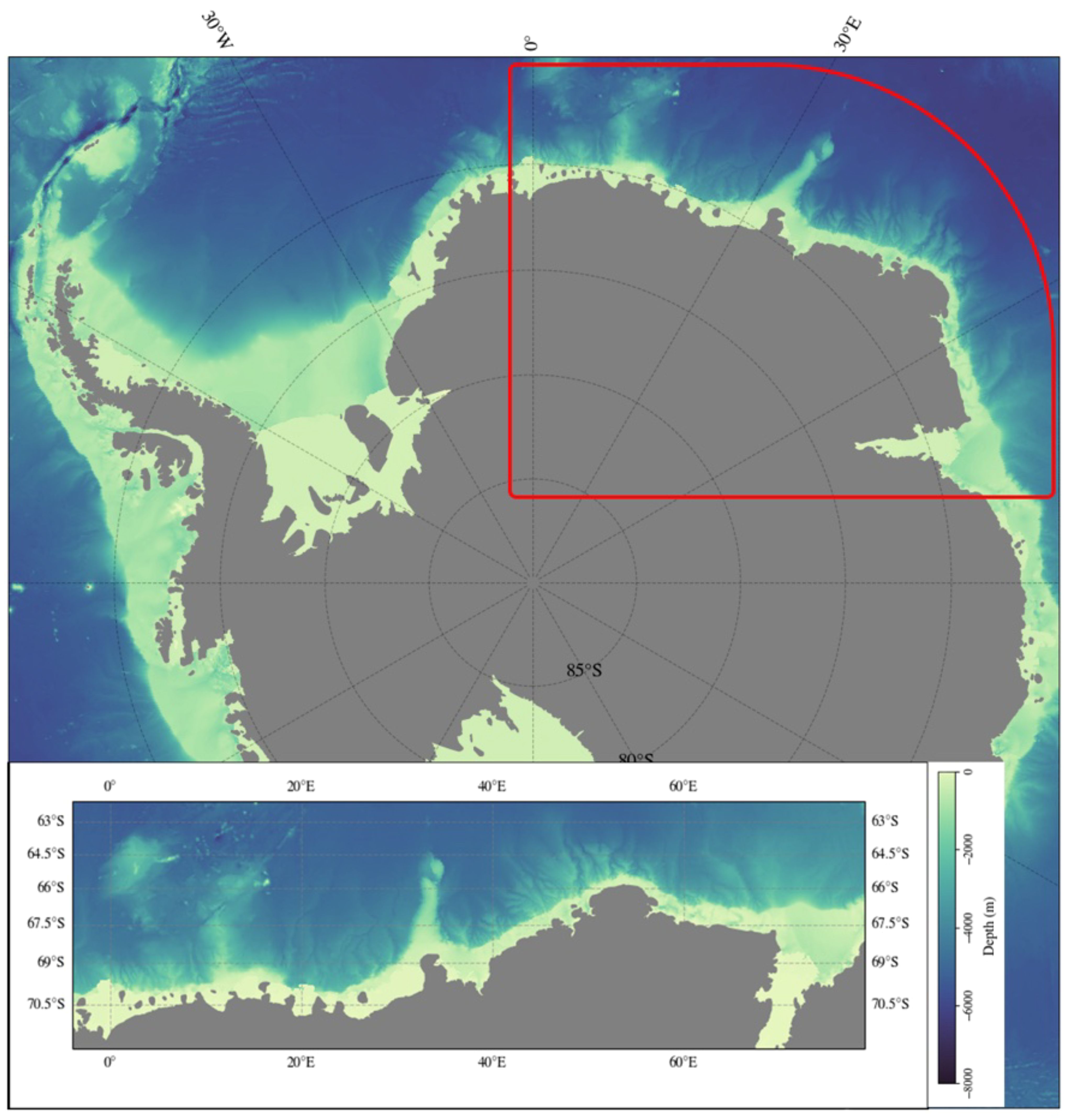
Figure 1. Overview map of the Antarctic region with a close-up of the study area.

These innovations collectively enable a more robust, scalable, and accurate eddy detection pipeline tailored to the unique environmental conditions of the Antarctic MIZ, positioning this work as a significant methodological advancement over previous efforts.

The paper is organized as follows: Section 2 provides details about the datasets and methods used in this study; Section 3 focuses on the obtained Experimental Results. The summary and conclusion are formulated in Section 4.

2 Datasets and methods

2.1 Datasets

2.1.1 Remote sensing data

Over recent decades, synthetic aperture radar (SAR) has become an indispensable remote sensing technology. It has significantly improved a wide range of applications. Currently, various SAR instruments orbit the Earth, operating across different frequency bands, polarization configurations, and spatial resolutions. One of SAR’s key advantages is its ability to provide reliable data under all weather and lighting conditions. This is particularly valuable in critical regions such as the polar areas, where optical sensors often fail to deliver complementary information. The combination of this capability with SAR’s high spatial resolution makes it especially effective for detecting oceanic phenomena, such as eddies in the marginal ice zone. However, interpreting SAR imagery remains challenging due to its complexity. Effective processing and analysis often require expert knowledge and experience.

This study focuses on the Sentinel-1 mission, widely utilized for its open-access data provided through the Copernicus Data Space Ecosystem, part of the European Union’s Earth observation program (ESA, 2024). The Sentinel-1 mission operates in the C-band with a central frequency of 5.404 GHz and includes polar-orbiting satellites Sentinel-1A, Sentinel-1B, and the recently launched Sentinel-1C. These satellites support multiple sensing modes tailored to various applications. For this research, we used data acquired in the extra-wide (EW) swath mode with dual polarization (HH and HV), a configuration commonly employed, particularly for sea ice monitoring. With a spatial resolution of 40 meters, this mode enables the identification of eddies of varying sizes and reveals complex details on the sea ice and ocean surface.

2.1.2 Dataset composition

To prepare the data for subsequent analysis, specifically, the automated detection of eddies in the MIZ, a series of preprocessing steps were applied. These included corrections for thermal and speckle noise, along with radiometric calibration to sigma nought values in dB, using the Sentinel Application Platform (SNAP) developed by the European Space Agency (ESA). The dataset consists of 234 scenes collected for 2018 and 2022, covering the whole year of the sea ice formation period, including ice development and melting. Additionally, the 115 scenes from MIZ of the Fram Strait region were added to the training sample. This data was partly collected for a case study on automatic eddy detection in the Arctic region Khachatrian et al. (2023) and partly for our current research on submesoscale dynamics in the Arctic MIZ (Sandalyuk and Khachatrian, 2025). Insertion of this data expanded our training sample and added additional variability patterns to the model training. Since the eddy vorticity sign changes in the Southern Hemisphere, it also helps balance the classes.

A subset of 14 scenes was reserved for testing, while the remaining scenes were divided into training and validation samples to evaluate model performance. It is worth mentioning that eddy signatures in the MIZ can vary depending on sensing parameters, geographic location, and environmental conditions. Hence, for the testing sample, we used only data from the Antarctic region.

To enhance eddy detection in SAR imagery, we employed a false-color composite approach. By combining the HV, HH, and HH bands into a composite representation, we improved the contrast and feature differentiation essential for identifying eddies in the MIZ. This technique leverages the distinct scattering properties captured by each polarization channel, accentuating subtle variations in sea ice cover and delineating the transition zone between open ocean and sea ice. The resulting false-color composite highlights eddy signatures by integrating surface roughness and scattering data, thereby facilitating more accurate and timely detection. This enhancement is particularly valuable for operational applications aimed at monitoring and understanding ice dynamics in near real-time.

2.2 Methodology

2.2.1 Overall framework of YOLO model

For automatic eddy detection in SAR imagery, we utilize the You Only Look Once (YOLO) model as a basic framework. YOLO is a one-stage state-of-the-art object detection model widely used for a wide range of object detection and classification tasks (Jocher et al., 2024). It has also proved to be an effective tool for eddy detection in SAR images in MIZ regions (Khachatrian et al., 2023), as well as in open ocean areas (Zi et al., 2024; Xia et al., 2022). In our work, we utilize the latest version of the YOLO model - YOLOv11, which incorporates various enhancements and provides better efficiency and optimized architecture in comparison with the previous versions. The basic structure of the YOLOv11 includes three modules: backbone, neck, and head (Jocher et al., 2024). The backbone module extracts features from the image at multiple scales. The neck is responsible for upsampling and concatenation of feature maps from different levels. On the head level, the final predictions are generated as a set of bounding boxes enclosing the objects on the image. More information regarding the specifics of the YOLOv11 architecture can be found at (Jocher et al., 2024).

2.2.2 Data augmentation

Data augmentation is a widely used technique in Machine Learning, which involves artificial expansion of the training dataset by generating new samples derived from the existing data. The use of various data augmentation techniques introduces additional variability into the training dataset. Given the limited training sample, we employ aggressive augmentation techniques during model training, including Hue/Saturation adjustments, Rotation, Mosaic transformations, Gaussian noise addition, and Copy-paste augmentation. During the fine-tuning process, the Mosaic augmentation technique has proven to be the most effective. Therefore, we set the probability of the Mosaic operation to 1, which means it was implemented in every training epoch.

We deliberately avoid certain widely used data augmentation techniques, such as Flip and Transpose. The reason for that is that the implementation of these settings will lead to changes in the eddies’ polarity, and consequently to the switching between classes. For example, if we flip an image containing CE horizontally or vertically, it becomes an AE, and vice versa. To tackle this problem, the flipping technique was implemented on the whole training dataset prior to training. Additionally, the corresponding labels were adjusted to align with the flipped images, and the classes were swapped accordingly. The resulting dataset was mixed with the main training dataset prior to model training. Flipping the training sample solved two problems at once: it significantly expanded the initial training dataset and balanced the two classes. Cyclonic eddies are usually more ubiquitous in the ocean, especially in the early stage of their life cycle (Chelton et al., 2011). This leads to the unequal representation of eddy polarities, which can also be observed in our dataset. We are aware that such an approach can lead to possible overfitting. However, no signs of model overfitting were observed after adding the flipped data to the training dataset.

2.2.3 Slicing aided hyper inference

During the model testing, we conducted additional experiments with the implementation of the Slicing Aided Hyper Inference (SAHI) module (Akyon et al., 2022). SAHI is designed to optimize the object detection process by splitting the image into separate overlapping tiles, running object detection on each slice, and finally merging slices back together into the resulting image. This effective technique allows for the enhancement of the detection of smaller objects on the satellite image. SAHI seamlessly integrated with the YOLOv11 model, offering easy implementation without requiring additional resources.

2.2.4 Geographical coordinates extraction

To extract actual geographical information of the detected eddies, we implement the affine transformation model, which converts pixel coordinates of the bounding boxes to their respective geographically referenced latitude and longitude coordinates (Warmerdam, 2008). We define the geometrical eddy center as the center of the bounding box that encloses the detected eddy. (Figure 2a) shows the geographical locations of the eddy centers, which were manually labeled for model training and validation.

Figure 2

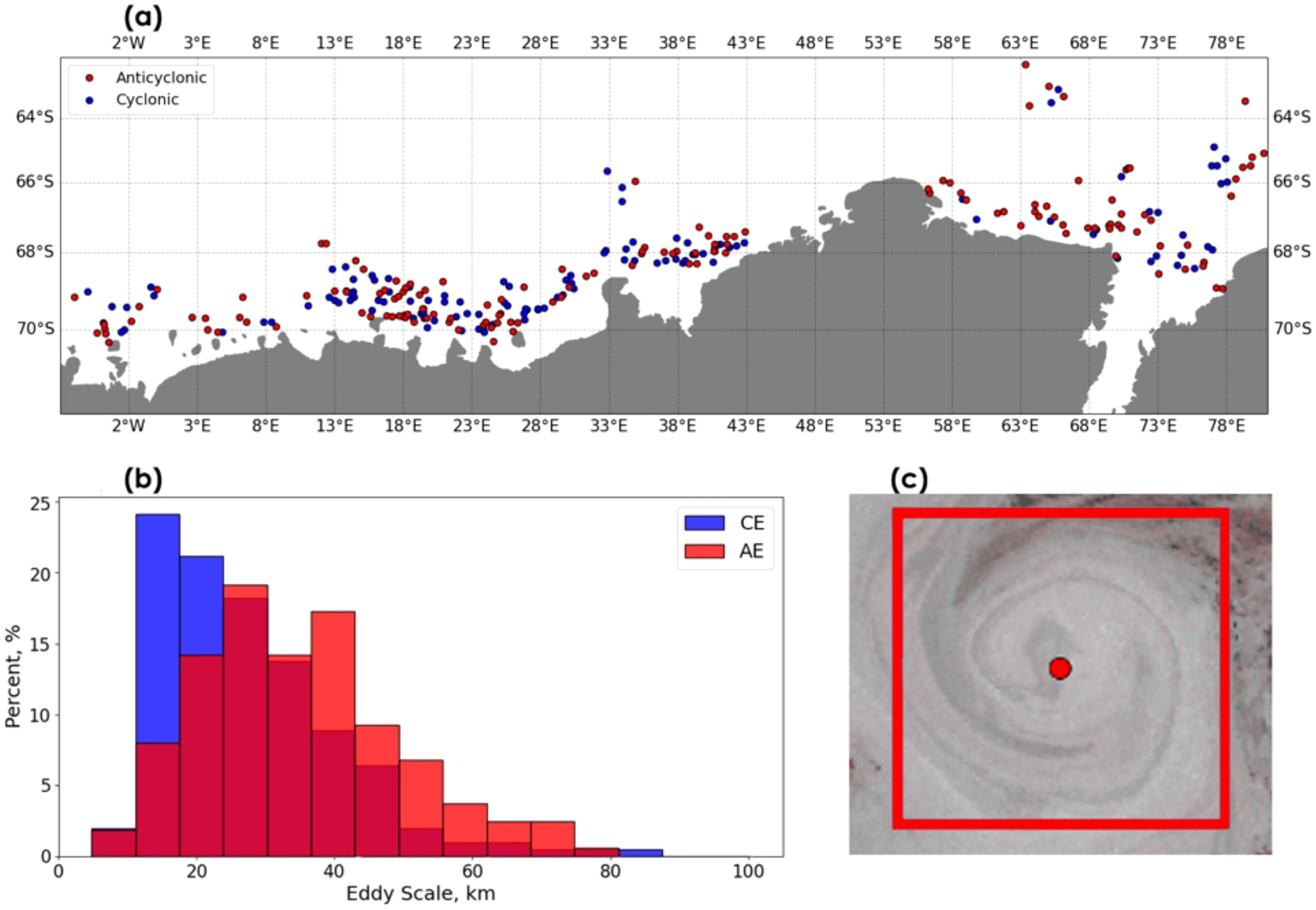
Figure 2. (a) Geographical position of the eddies acquired for the training and validation dataset; (b) Histogram distributions of the number of eddies and their scales; (c) The example of anticyclonic eddy center (red dot), obtained from the geographical coordinates extraction module.

Additionally, we compute the eddy spatial scale (Figure 2b). Following the assumption that generally eddies have an elliptical shape (Chen et al., 2019; Bashmachnikov et al., 2020), we define the eddy scale as an average of the lengths of the major and minor axes, which in our case corresponds to the average of the sum of the height and width of the eddy bounding box. The utilized approach for eddy spatial scale definition has been previously implemented in several studies (Kozlov et al., 2019b, a; Kozlov and Atadzhanova, 2022; Zi et al., 2024). Eddy spatial scales range from around 2.5 to 85 km. (Figure 2b). The cyclones have a peak in the scale range of 10–15 km. At this scale, cyclones strongly dominate over anticyclones. However, starting from the scale values above 25 km, anticyclones are predominant.

2.2.5 Evaluation Metrics

We assess the YOLO model’s performance using standard detection metrics: precision, recall, and mean average precision (mAP). The precision and recall metrics are defined according to the Equations 1, 2 where TP, FP, and FN are the number of true positive, false positive, and false negative predictions, respectively. TP is a correctly identified eddy, FP occur when non-eddy features are misclassified as eddies, while FN represent missed eddies. Precision reflects the ratio of true positives to all eddy predictions, whereas recall indicates the model’s ability to capture all genuine eddy occurrences in the data.

$\begin{array}{ll}\mathrm{Precision}=\frac{TP}{TP+FP}& (1)\end{array}$

$\begin{array}{ll}\mathrm{Recall}=\frac{TP}{TP+FN}& (2)\end{array}$

The AP (Equation 3) and mAP (Equation 4) indicate an optimal trade-off between precision and recall:

$\begin{array}{ll}AP={\displaystyle {\int }_0^{1}P(R)dR}& (3)\end{array}$

$\begin{array}{ll}mAP=\frac{{\sum }_{i=1}^{n}A{P}_i}{n}& (4)\end{array}$

where R is recall, P(R) is a function of recall, n is the number of classes being averaged. P(R) represents precision as a function of recall. The mAP (Equation 4) is usually calculated for a specific confidence level, which in our case is defined by the Intersection over Union (IoU) value. The IoU measures the level of overlap between the predicted and the ground-truth bounding boxes. The IoU thresholds of 0.5 (mAP_0.5) and threshold range of 0.5-0.95 (mAP_0.5−0.95) were employed for model evaluation. The main goal during the model training and tuning was the minimization of the number of false positive detections. This approach is preferable to alternatives that maximize recall at the expense of precision, as it avoids false detections of filamentary structures and other eddy-like features that could compromise quantitative analyses. Additionally, the visual inspection of every detection result for every image from the validation and test datasets was conducted.

3 Experimental results

3.1 Validation sample evaluation

Figure 3 displays examples of the YOLOv11 model’s outputs for validation samples taken from the same region, captured on February 01, 2018, and February 10, 2018. In these images, bounding boxes denote detected eddy signatures categorized as blue for cyclonic eddies, red for anticyclonic eddies (blue and red correspond to initially labeled and detected signatures), and yellow for eddies that were either misclassified or not initially labeled but detected by the algorithm.

Figure 3

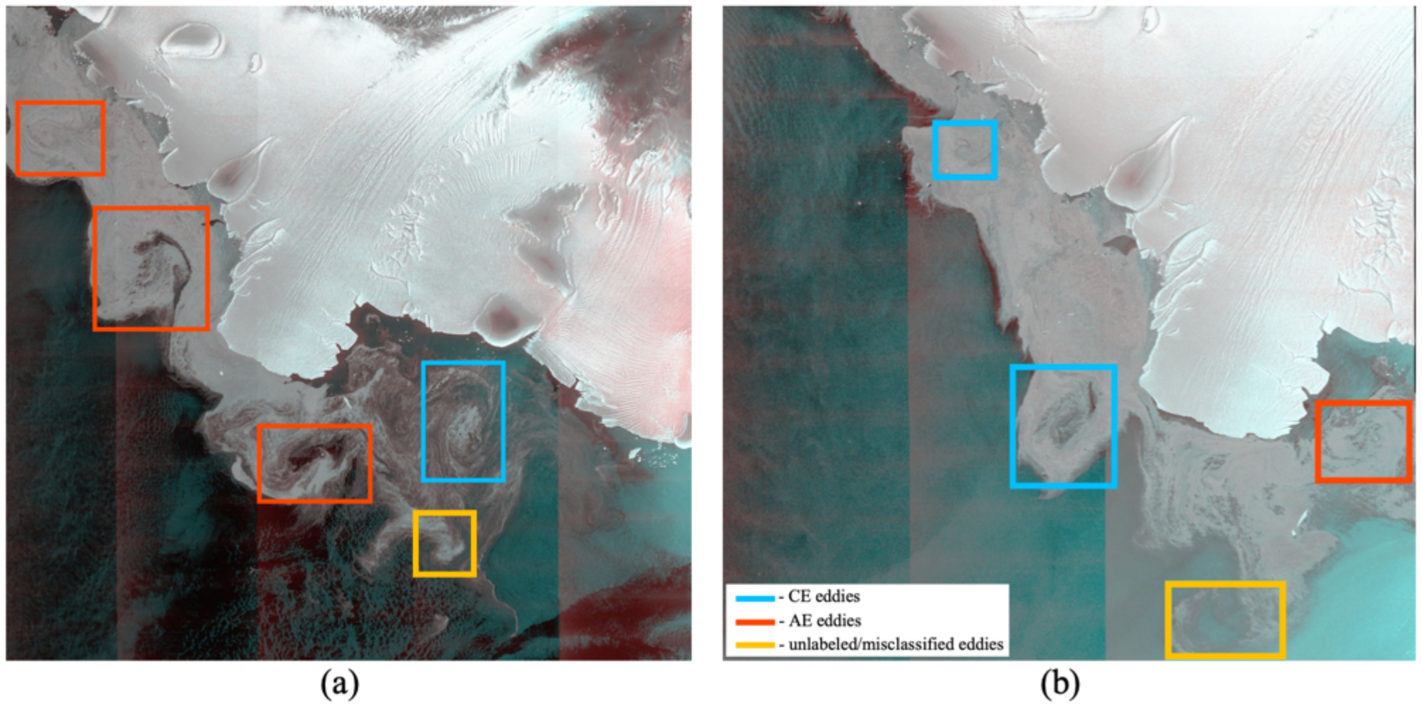
Figure 3. Examples of the YOLOv11 model’s outputs showing detected eddies within the MIZ from validation samples acquired on (a) February 01, 2018, and (b) February 10, 2018. Rectangles indicate identified eddy signatures: blue for cyclonic eddies that were both initially labeled and detected by the algorithm, red for anticyclonic eddies that were both initially labeled and detected by the algorithm, and yellow for eddies that were either misclassified or not initially labeled but detected by the algorithm.

The YOLOv11 model demonstrates strong performance in detecting submesoscale and mesoscale eddies within the MIZ, effectively identifying both cyclonic and anticyclonic features. In the first image (a), the model successfully detected an additional cyclonic eddy that was not initially labeled. This newly identified eddy appears accurate upon inspection and is notable for being in an early developmental stage compared to the more established eddies present in the scene. This highlights the model’s capability to recognize smaller-scale or less-developed features, which might be overlooked during manual labeling.

In contrast, the second image (b) shows a case where the algorithm missed a cyclonic eddy signature present in the initial labels. Despite this, the majority of the detected eddy signatures align with their respective categories, underscoring the model’s overall accuracy and consistency in identifying mesoscale eddies.

The side-by-side comparison of validation scenes illustrates both the strengths and limitations of the YOLOv11 model, offering valuable insights into its ability to capture dynamic eddy behavior over time and its sensitivity to changes in eddy characteristics.

3.2 Test sample evaluation

Figure 4 displays the YOLOv11 model’s outputs, illustrating eddy detection within the study region and providing a compelling demonstration of its capability to identify and classify eddies in diverse sea ice conditions. Each test image from December 23, February 01, and April 10, 2022, showcases distinct scenarios with varying levels of sea ice concentration and eddy dynamics.

Figure 4

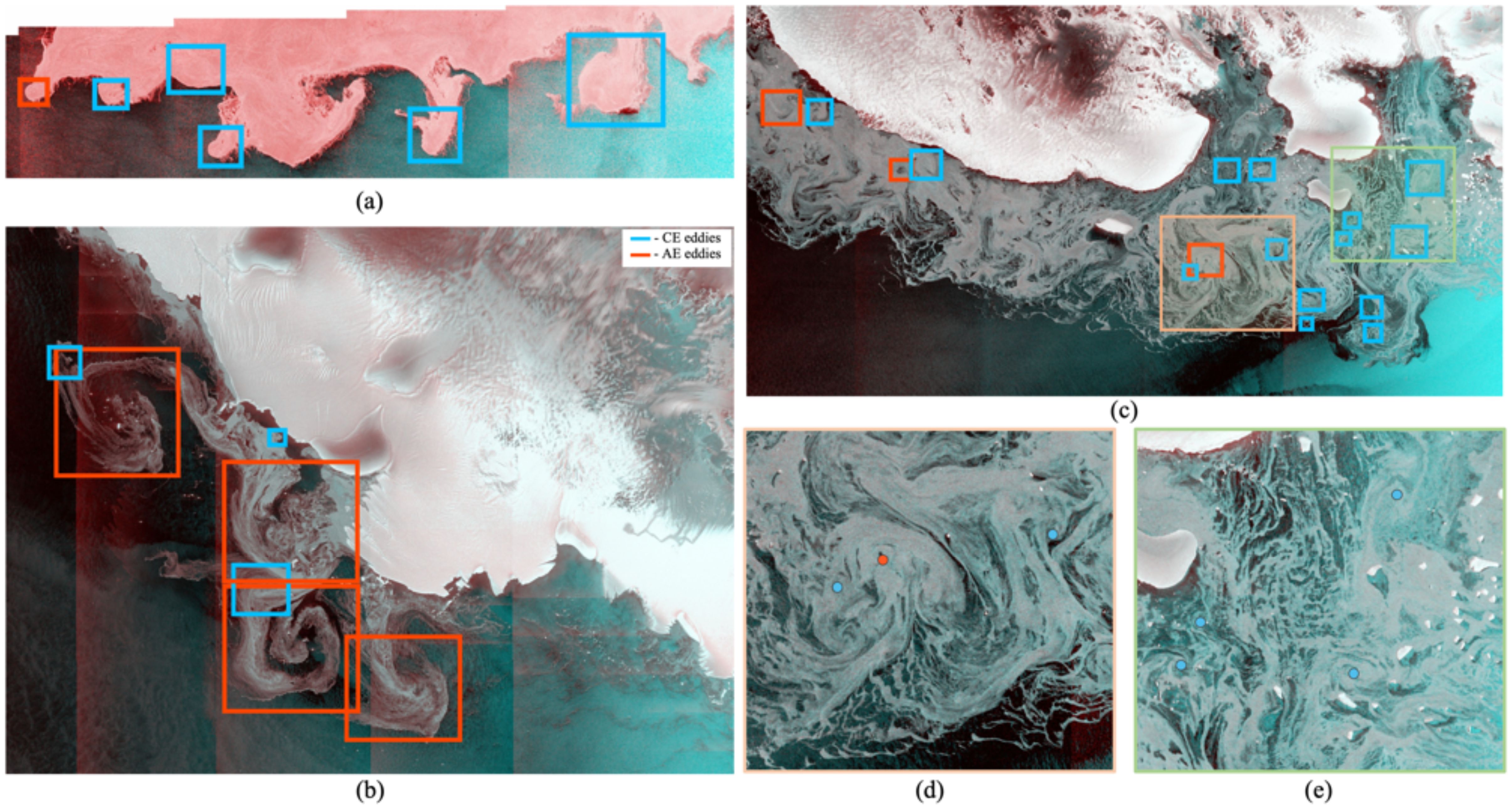
Figure 4. Examples of the YOLOv11 model’s outputs showing detected eddies within the MIZ from test data acquired on (a) December 23, (b) February 01, and (c) April 10, 2022. Rectangles indicate identified eddy signatures (blue for cyclonic, red for anticyclonic). Images (d, e) provide zoomed-in views of smaller-scale eddy dynamics in the MIZ, which exhibit highly chaotic behavior, as highlighted in image (c). Circles refer to the approximate eddy centers.

Figure 4a highlights the very edge of the MIZ, where sea ice concentration is notably high and observed eddies are densely packed in the ice field. The detected eddies in this region are in their early developmental stages but remain distinct and identifiable. The algorithm successfully identifies most eddies, demonstrating its robustness even in challenging high-concentration ice zones. However, one potential eddy on the right, which appears similar to the detected instances, is not identified. This feature might represent an eddy in an even earlier developmental stage, which has not yet formed a fully circular pattern and thereby explains the exclusion from detection by the model.

Figure 4b illustrates a scenario with reduced sea ice concentration compared to (a), revealing a mix of large anticyclonic eddies, approximately 50 km in diameter, and smaller cyclonic eddies. The YOLOv11 model performs admirably in this environment, correctly identifying all eddies and their polarities without misclassification. This scene underscores the algorithm’s precision in detecting eddy features across varying scales and contrasts, even in less congested ice fields. Nevertheless, the overall performance remains highly effective and reliable.

Figure 4c demonstrates a chaotic, smaller-scale eddy dynamic within the MIZ, capturing the intricate and turbulent nature of the environment. This complexity is emphasized in the zoomed-in views provided in Figures 4d, e, which focus on the finer-scale eddies present within the region. Despite the highly chaotic behavior exhibited in this dataset, the model continues to perform reliably, accurately detecting and distinguishing between cyclonic and anticyclonic eddies. These results demonstrate the model’s resilience and adaptability to challenging conditions.

Combined, these three images showcase the YOLOv11 model’s capacity to analyze and interpret exceptionally different sea ice scenarios. From high-concentration zones with dense sea ice fields to chaotic dynamics, the algorithm effectively identifies eddies and their polarities, proving its robustness across a range of conditions. While minor challenges remain, the overall performance indicates that the model is a valuable tool for studying eddy dynamics in the MIZ. The final metrics obtained during the model testing are presented in Table 1.

Table 1

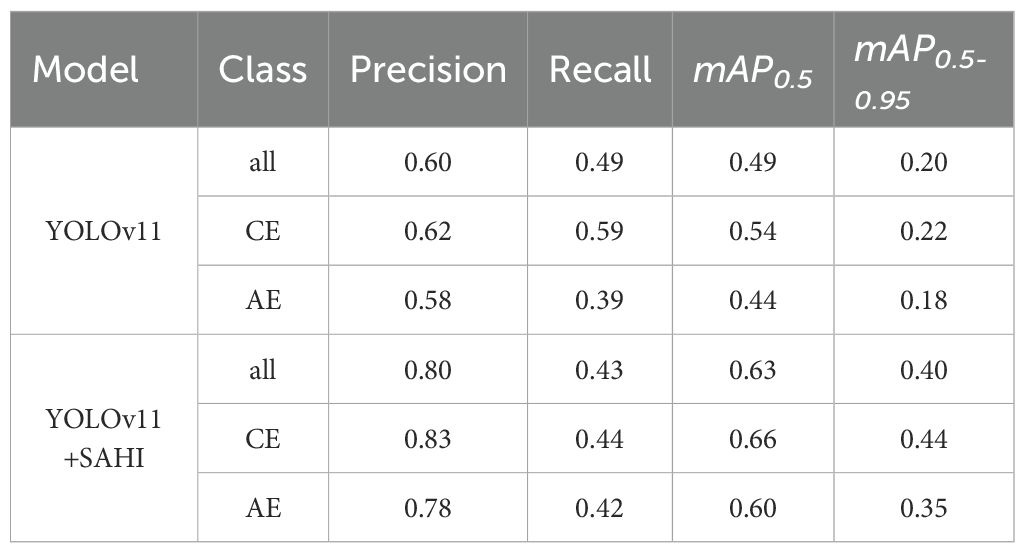
Table 1. Overview of performance evaluation metrics for multi-class model.

3.3 Enhancing eddy detection with SAHI

Figure 5 illustrates the outputs of the YOLOv11 model with the implementation of the SAHI module, showing detected eddies within the MIZ, based on test data acquired on December 23, February 01, and April 10, 2022.

Figure 5

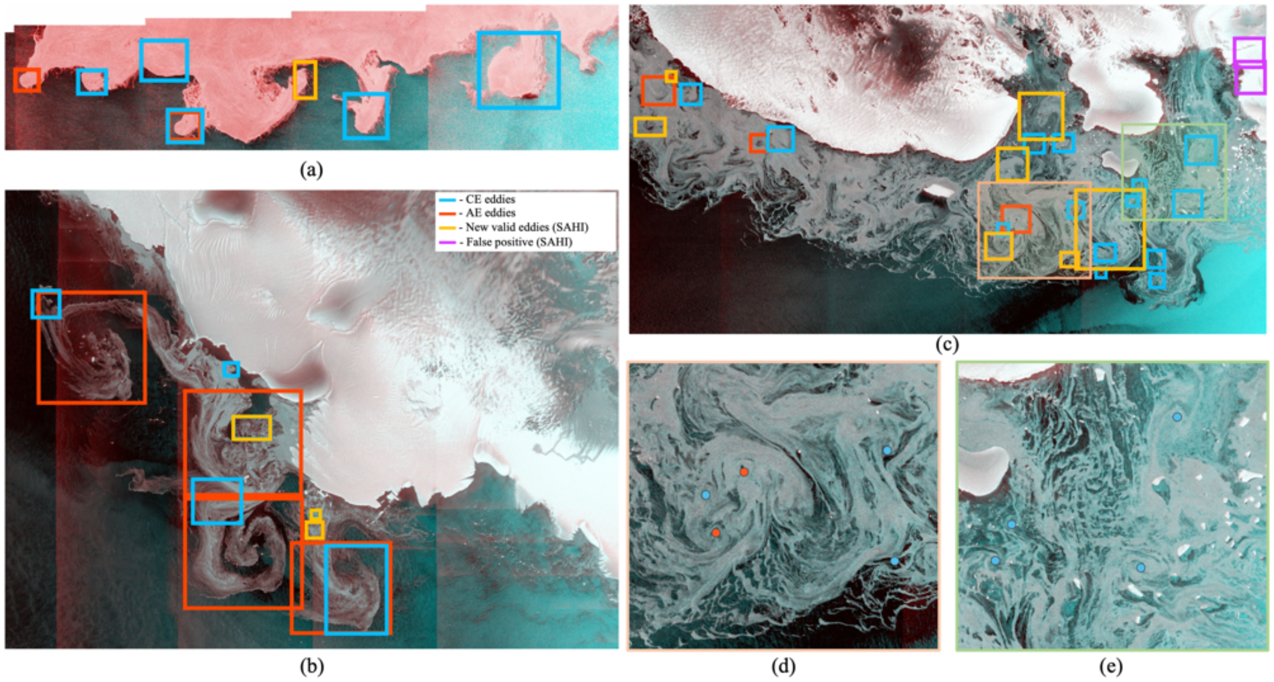
Figure 5. Examples of YOLOv11 model outputs using the SAHI module to detect eddies within the MIZ from test data acquired on (a) December 23, (b) February 01, and (c) April 10, 2022. Images (d, e) provide zoomed-in views of smaller-scale eddy dynamics in the MIZ. Blue and red rectangles correspond to cyclonic and anticyclonic eddies detected by YOLOv11 alone, as shown in Figure 4. Yellow rectangles indicate additional valid detections made by the SAHI module that were missed previously, while purple rectangles represent false positives introduced by SAHI.

It should be noted that the SAHI module has two basic settings: the height and width of the slice, and the overlap height and width ratio. Variations of these settings can significantly affect the final output, either decreasing the accuracy of eddy detection or leading to excessive detection of small features. Both scenarios result in a decline in overall metrics. After conducting a series of experimental runs, we identified the optimal combination of SAHI settings, which optimizes the detection of the small mesoscale eddies in the MIZ without compromising the overall quality. The updated results with SAHI demonstrate its potential to enhance object detection in complex and dynamic environments, as well as improve the detection of smaller-scale eddies, with noteworthy observations for each test case.

For the data acquired on December 23, 2022, there were minimal changes compared to the results without SAHI. The addition of one previously missed anticyclonic eddy highlighted an improvement in sensitivity. However, a limitation of the algorithm emerged when one eddy was simultaneously detected as both cyclonic and anticyclonic, revealing a potential conflict or ambiguity in detection. Overall, SAHI maintained the accuracy of the original model while marginally improving its ability to identify smaller features.

In the case of February 01, 2022, the majority of eddies detected matched those identified without the use of SAHI. Importantly, SAHI enabled the detection of smaller-scale eddies that were missed in the previous iteration, confirming its utility for identifying finer details. Similar to the December 23 results, one eddy was misclassified as both cyclonic and anticyclonic, indicating the need for better handling of overlapping or ambiguous features within the algorithm.

The results for April 10, 2022, demonstrated significant improvements with SAHI. The model detected more eddies in the highly dynamic and chaotic eddy field, underscoring SAHI’s ability to resolve complex spatial features. However, two cyclonic eddies were incorrectly identified on land. This misclassification points to a lack of geographical awareness in the model. One of the key features of the study region is the close proximity of the Antarctic ice sheet, which is present in almost every scene. In some cases, the glaciers exhibit circular patterns that can be misidentified by the model as eddies. This issue is illustrated in Figure 4c at the upper right corner (purple rectangles), where two marked false detections over the glacier/land can be seen. Nonetheless, this limitation is not critical, as it can be effectively addressed by incorporating a land mask. Despite this issue, the ability to detect additional instances in such a dynamic environment reflects the considerable potential of SAHI.

After SAHI implementation the Precision and mAP_0.5 values increased by the ~ 25% (Table 1), with the mAP_0.5–0.95 increased by 50% in comparision with the baseline YOLOv11 model. At the same time, the overall Recall value slightly decreased after the inclusion the SAHI in the detection process. The observed recall reduction likely occurs because some eddies located near slice overlap regions are either undetected or truncated during the slicing process.

In conclusion, the integration of SAHI with YOLOv11 demonstrates its capability to improve object detection by capturing smaller and more complex features, particularly in dynamic environments. SAHI enhances the sensitivity of the model to the small submesoscale structures while maintaining accuracy in simpler cases. However, it also highlights the need for refinement to address issues such as conflicting classifications and misdetections on land. The performance improvements achieved with SAHI suggest it has significant potential to enhance object detection workflows, especially when paired with supplementary modules like geographical masks. However, we did not apply a land mask in this study, as we aimed to clearly illustrate both the advantages and limitations of SAHI. This currently represents a limitation that could be addressed in future work.

4 Summary and conclusion

This work presents the first attempt to implement a machine learning approach for automatic eddy identification in the Antarctic MIZ region, as well as the first assessment of eddy dynamics using SAR images in this area. While the present study focuses on the Antarctic, the methodology builds upon our previous developments and applications in the Arctic MIZ (Khachatrian et al., 2023; Sandalyuk and Khachatrian, 2025), demonstrating its adaptability across polar environments. These prior studies highlight the robustness of YOLO-based eddy detection from Sentinel-1 SAR data, providing a solid foundation for extending the approach to different polar regions and for potential integration into operational sea ice and ocean monitoring systems.

The Antarctic MIZ is a region characterized by the highly intense dynamical processes that have a major influence on the atmosphere–ice-ocean interactions, heat and salt transport, and biological productivity. Moreover, this region remains a major source of uncertainty in eddy-resolving models, due to the sparse in situ measurements, presence of sea ice, and, specifically, limited data on the eddy dynamics (Tietsche et al., 2014). In our study, we took the first steps toward developing a robust tool for obtaining high-quality data on eddy characteristics in this region.

During the data collection and image labeling for training and validating the model, we collected extensive information on the locations and sizes of mesoscale and submesoscale eddies in the MIZ of the study area. As no prior research has been done in this area, these findings represent valuable new insights. We can observe a dense, wide band of eddy detections, resulting from the seasonal and inter-annual variability of the sea ice edge (Figure 2). It is evident from the experimental results that the study region presents a hot spot of MIZ eddy generation. The possible eddy generation mechanism and eddy influence on the location of the ice edge will be the main focus of future research.

Our research demonstrates the efficiency of YOLOv11, a state-of-the-art deep learning model, in detecting and classifying oceanic eddies within the Antarctic MIZ using high-resolution SAR imagery. By finetuning YOLOv11 on training and validation datasets, we successfully identified both submesoscale and mesoscale eddies across diverse sea ice conditions, achieving robust performance in distinguishing cyclonic and anticyclonic eddies. These advancements represent a vital step in the automated study of Antarctic oceanographic processes, an area that has remained largely unexplored compared to the more extensive efforts conducted in the Arctic.

The experimental results highlight the adaptability and accuracy of the YOLOv11 model. It performed reliably across varying ice concentrations and eddy dynamics, from high-concentration zones to chaotic, small-scale eddy fields. While the base model demonstrated considerable strength, the integration of the SAHI module further improved its performance, particularly in detecting smaller and more complex features. Notably, SAHI enhanced sensitivity and accuracy in dynamic environments, revealing additional eddies and capturing finer-scale dynamics that were previously overlooked.

Despite the robust performance, certain challenges were identified. A recurring issue was the occasional misclassification of eddies as both cyclonic and anticyclonic, reflecting ambiguities in detection under specific conditions. Additionally, the misidentification of eddies on land during SAHI-enabled inference underscores the need for the potential integration of additional features, such as the incorporation of a land mask. These limitations highlight opportunities for future refinement of the model architecture and supporting workflows.

The findings of this study underline the potential of deep learning models like YOLOv11, particularly when integrated with modules such as SAHI, for advancing polar oceanography. By enabling more detailed and accurate analysis of eddy dynamics in the Antarctic MIZ, this research lays the groundwork for compiling comprehensive statistical datasets and improving our understanding of polar climate systems. Future efforts could focus on addressing the identified limitations, exploring complementary datasets, and enhancing model robustness to ensure consistent performance across a broader range of environmental scenarios.

Overall, this work bridges a critical gap in Antarctic eddy research, providing a scalable and automated solution for studying these vital oceanographic features. The success of the YOLOv11 model and its integration with SAHI points to promising directions for further research, offering a pathway to more comprehensive and efficient studies of dynamic polar systems. As a potential future step, the authors intend to make publicly available the training dataset and YOLOv11 configuration after obtaining data on inter-annual variability and statistics on eddy occurrences for the study region.

Data availability statement

The Sentinel-1 data are publicly available through Copernicus Data Space Ecosystem (https://dataspace.copernicus.eu/) after registration. The YOLOv11 model is freely available at https://github.com/ultralytics/ultralytics.

Author contributions

NS: Conceptualization, Data curation, Formal Analysis, Visualization, Writing – original draft, Writing – review & editing. EK: Conceptualization, Data curation, Formal Analysis, Visualization, Writing – original draft, Writing – review & editing. EM: Data curation, Writing – original draft, Writing – review & editing.

Funding

The author(s) declare financial support was received for the research and/or publication of this article. This research was funded by the Moscow Institute of Physics and Technology under the Agreement No. 075-03-2024–117 dated January 17, 2024, and The Arctic University of Norway. Ekaterina Marchuk is supported by the state assignment of the A.M. Obukhov Institute of Atmospheric Physics RAS (FMWR125020501524-9).

Conflict of interest

The authors declare that the research was conducted in the absence of any commercial or financial relationships that could be construed as a potential conflict of interest.

Generative AI statement

The author(s) declare that no Generative AI was used in the creation of this manuscript.

Any alternative text (alt text) provided alongside figures in this article has been generated by Frontiers with the support of artificial intelligence and reasonable efforts have been made to ensure accuracy, including review by the authors wherever possible. If you identify any issues, please contact us.

Publisher’s note

All claims expressed in this article are solely those of the authors and do not necessarily represent those of their affiliated organizations, or those of the publisher, the editors and the reviewers. Any product that may be evaluated in this article, or claim that may be made by its manufacturer, is not guaranteed or endorsed by the publisher.

References

Akyon F. C., Altinuc S. O., and Temizel A. (2022). “Slicing aided hyper inference and fine-tuning for small object detection,” in 2022 IEEE international conference on image processing (ICIP), (Bordeaux, France) 966–970. doi: 10.1109/ICIP46576.2022.9897990

Crossref Full Text | Google Scholar

Auger M., Sallée J.-B., Prandi P., and Naveira Garabato A. C. (2022). Subpolar southern ocean seasonal variability of the geostrophic circulation from multi-mission satellite altimetry. J. Geophysical Research: Oceans 127, e2021JC018096. doi: 10.1029/2021JC018096

Crossref Full Text | Google Scholar

Auger M., Sallée J.-B., Thompson A. F., Pauthenet E., and Prandi P. (2023). Southern ocean ice-covered eddy properties from satellite altimetry. J. Geophysical Research: Oceans 128, e2022JC019363. doi: 10.1029/2022JC019363

Crossref Full Text | Google Scholar

Bashmachnikov I., Kozlov I., Petrenko L., Glock N., and Wekerle C. (2020). Eddies in the north Greenland sea and fram strait from satellite altimetry, sar and high-resolution model data. J. Geophysical Research: Oceans. 125, e2019JC015832. doi: 10.1029/2019JC015832

Crossref Full Text | Google Scholar

Bennetts L. G., Shakespeare C. J., Vreugdenhil C. A., Foppert A., Gayen B., Meyer A., et al. (2024). Closing the loops on southern ocean dynamics: From the circumpolar current to ice shelves and from bottom mixing to surface waves. Rev. Geophysics 62, e2022RG000781. doi: 10.1029/2022RG000781

Crossref Full Text | Google Scholar

Biddle L. C. and Swart S. (2020). The observed seasonal cycle of submesoscale processes in the antarctic marginal ice zone. J. Geophysical Research: Oceans 125, e2019JC015587. doi: 10.1029/2019JC015587

Crossref Full Text | Google Scholar

Bitz C. M., Gent P. R., Woodgate R. A., Holland M. M., and Lindsay R. (2006). The influence of sea ice on ocean heat uptake in response to increasing co2. . J. Climate 19, 2437 –2450. doi: 10.1175/JCLI3756.1

Crossref Full Text | Google Scholar

Boccaletti G., Ferrari R., and Fox-Kemper B. (2007). Mixed layer instabilities and restratification. J. Phys. Oceanography 37, 2228–2250. doi: 10.1175/JPO3101.1

Crossref Full Text | Google Scholar

Bondevik E. (2011). Studies of eddies in the marginal ice zone along the east Greenland current using spaceborne synthetic aperture radar (SAR). (Master’s Thesis). The University of Bergen, Bergen, Norway. 95p.

Google Scholar

Chelton D. B., Schlax M. G., and Samelson R. M. (2011). Global observations of nonlinear mesoscale eddies. Prog. Oceanography 91, 167–216. doi: 10.1016/j.pocean.2011.01.002

Crossref Full Text | Google Scholar

Chen G., Han G., and Yang X. (2019). On the intrinsic shape of oceanic eddies derived from satellite altimetry. Remote Sens. Environ. 228, 75–89. doi: 10.1016/j.rse.2019.04.011

Crossref Full Text | Google Scholar

Davis C. H., Li Y., McConnell J. R., Frey M. M., and Hanna E. (2005). Snowfall-driven growth in east antarctic ice sheet mitigates recent sea-level rise. Science 308, 1898–1901. doi: 10.1126/science.1110662

PubMed Abstract | Crossref Full Text | Google Scholar

Depoorter M. A., Bamber J. L., Griggs J. A., Lenaerts J. T. M., Ligtenberg S. R. M., van den Broeke M. R., et al. (2013). Calving fluxes and basal melt rates of antarctic ice shelves. Nature 502, 89–92. doi: 10.1038/nature12567

PubMed Abstract | Crossref Full Text | Google Scholar

DeVries T. (2014). The oceanic anthropogenic co2 sink: Storage, air-sea fluxes, and transports over the industrial era. Global Biogeochemical Cycles 28, 631–647. doi: 10.1002/2013GB004739

Crossref Full Text | Google Scholar

Dotto T. S., Naveira Garabato A., Bacon S., Tsamados M., Holland P. R., Hooley J., et al. (2018). Variability of the ross gyre, southern ocean: Drivers and responses revealed by satellite altimetry. Geophysical Res. Lett. 45, 6195–6204. doi: 10.1029/2018GL078607

Crossref Full Text | Google Scholar

Du Y., Liu J., Song W., He Q., and Huang D. (2019). Ocean eddy recognition in sar images with adaptive weighted feature fusion. IEEE Access 7, 152023–152033. doi: 10.1109/ACCESS.2019.2946852

Crossref Full Text | Google Scholar

du Plessis M., Swart S., Ansorge I. J., Mahadevan A., and Thompson A. F. (2019). Southern ocean seasonal restratification delayed by submesoscale wind–front interactions. J. Phys. Oceanography 491035–1053. doi: 10.1175/JPO-D-18-0136.1

Crossref Full Text | Google Scholar

ESA (2024). Sentinel-1 level 1 EW GRD products. Available online at: https://dataspace.copernicus (Accessed 18-April-2024).

Google Scholar

Fox-Kemper B., Ferrari R., and Hallberg R. (2008). Parameterization of mixed layer eddies. part i: Theory and diagnosis. J. Phys. Oceanography 381145–1165. doi: 10.1175/2007JPO3792.1

Crossref Full Text | Google Scholar

Frölicher T. L., Sarmiento J. L., Paynter D. J., Dunne J. P., Krasting J. P., and Winton M. (2015). Dominance of the southern ocean in anthropogenic carbon and heat uptake in cmip5 models. J. Climate 28, 862–886. doi: 10.1175/JCLI-D-14-00117.1

Crossref Full Text | Google Scholar

Gille S. T. (1997). The southern ocean momentum balance: Evidence for topographic effects from numerical model output and altimeter data. J. Phys. Oceanography 27, 2219–2232. doi: 10.1175/1520-0485(1997)027h2219:TSOMBEi2.0.CO;2

Crossref Full Text | Google Scholar

Greene C. A., Gardner A. S., Schlegel N.-J., and Fraser A. D. (2022). Antarctic calving loss rivals ice-shelf thinning. Nature 609, 948–953. doi: 10.1038/s41586-022-05037-w

PubMed Abstract | Crossref Full Text | Google Scholar

Horvat C., Tziperman E., and Campin J. (2016). Interaction of sea ice floe size, ocean eddies, and sea ice melting. Geophysical Res. Lett. 43, 8083–8090. doi: 10.1002/2016gl069742

Crossref Full Text | Google Scholar

Ivchenko V. O., Danilov S., and Olbers D. (2008). Eddies in numerical models of the Southern Ocean (American Geophysical Union) 177–198. doi: 10.1029/177gm13

Crossref Full Text | Google Scholar

Jayne S. R. and Marotzke J. (2002). The oceanic eddy heat transport. J. Phys. Oceanography 32, 3328–3345. doi: 10.1175/1520-0485(2002)032h3328:TOEHTi2.0.CO;2

Crossref Full Text | Google Scholar

Jocher G., Chaurasia A., and Qiu J. (2024). Ultralytics yolov8. Available online at: https://github.com/ultralytics/ultralytics (Accessed December 15, 2024).

Google Scholar

Johannessen O. M., Johannessen J. A., Svendsen E., Shuchman R. A., Campbell W. J., and Josberger E. (1987). Ice-edge eddies in the fram strait marginal ice zone. Science 236, 427–429. doi: 10.1126/science.236.4800.427

PubMed Abstract | Crossref Full Text | Google Scholar

Khachatrian E., Sandalyuk N., and Lozou P. (2023). Eddy detection in the marginal ice zone with sentinel-1 data using yolov5. Remote Sens. 15. doi: 10.3390/rs15092244

Crossref Full Text | Google Scholar

Kirkman C. H. and Bitz C. M. (2011). The effect of the sea ice freshwater flux on southern ocean temperatures in ccsm3: Deep-ocean warming and delayed surface warming. J. Climate 24, 2224–2237. doi: 10.1175/2010jcli3625.1

Crossref Full Text | Google Scholar

Kozlov I. E., Artamonova A. V., Manucharyan G. E., and Kubryakov A. A. (2019b). Eddies in the western arctic ocean from spaceborne sar observations over open ocean and marginal ice zones. J. Geophysical Research: Oceans 124, 6601–6616. doi: 10.1029/2019JC015113

Crossref Full Text | Google Scholar

Kozlov I. E. and Atadzhanova O. A. (2022). Eddies in the marginal ice zone of fram strait and svalbard from spaceborne sar observations in winter. Remote Sens. 14. doi: 10.5194/egusphere-egu22-3711

Crossref Full Text | Google Scholar

Kozlov I. E., Petrenko L. A., and Plotnikov E. V. (2019a). Statistical and dynamical properties of ocean eddies in fram strait from spaceborne sar observations. Remote Sens. 2019, 111500S. doi: 10.1117/12.2533317

Crossref Full Text | Google Scholar

Kozlov I. E., Plotnikov E. V., and Manucharyan G. E. (2020). Brief communication: Mesoscale and submesoscale dynamics in the marginal ice zone from sequential synthetic aperture radar observations. Cryosphere 14, 2941–2947. doi: 10.5194/tc-14-2941-2020

Crossref Full Text | Google Scholar

Liu Y., Moore J. C., Cheng X., Gladstone R. M., Bassis J. N., Liu H., et al. (2015). Ocean-driven thinning enhances iceberg calving and retreat of antarctic ice shelves. Proc. Natl. Acad. Sci. 112, 3263–3268. doi: 10.1073/pnas.1415137112

PubMed Abstract | Crossref Full Text | Google Scholar

Lu K., Weingartner T., Danielson S., Winsor P., Dobbins E., Martini K., et al. (2015). Lateral mixing across ice meltwater fronts of the chukchi sea shelf. Geophysical Res. Lett. 42, 6754–6761. doi: 10.1002/2015GL064967

Crossref Full Text | Google Scholar

Mahadevan A., D’Asaro E., Lee C., and Perry M. J. (2012). Eddy-driven stratification initiates north atlantic spring phytoplankton blooms. Science 337, 54–58. doi: 10.1126/science.1218740

PubMed Abstract | Crossref Full Text | Google Scholar

Manucharyan G. E. and Thompson A. F. (2017). Submesoscale sea ice-ocean interactions in marginal ice zones. J. Geophysical Research: Oceans 122, 9455–9475. doi: 10.1002/2017JC012895

Crossref Full Text | Google Scholar

Marshall G. J. (2003). Trends in the southern annular mode from observations and reanalyses. J. Climate 164134–4143. doi: 10.1175/1520-0442(2003)016h4134:TITSAMi2.0.CO;2

Crossref Full Text | Google Scholar

Mizobata K., Shimada K., Aoki S., and Kitade Y. (2020). The cyclonic eddy train in the Indian ocean sector of the southern ocean as revealed by satellite radar altimeters and in situ measurements. J. Geophysical Research: Oceans 125, e2019JC015994. doi: 10.1029/2019JC015994

Crossref Full Text | Google Scholar

Palóczy A., Gille S. T., and McClean J. L. (2018). Oceanic heat delivery to the antarctic continental shelf: Large-scale, low-frequency variability. J. Geophysical Research: Oceans 123, 7678–7701. doi: 10.1029/2018JC014345

Crossref Full Text | Google Scholar

Pritchard H. D., Arthern R. J., Vaughan D. G., and Edwards L. A. (2009). Extensive dynamic thinning on the margins of the Greenland and antarctic ice sheets. Nature 461, 971–975. doi: 10.1038/nature08471

PubMed Abstract | Crossref Full Text | Google Scholar

Rignot E., Jacobs S., Mouginot J., and Scheuchl B. (2013). Ice-shelf melting around Antarctica. Science 341, 266–270. doi: 10.1126/science.1235798

PubMed Abstract | Crossref Full Text | Google Scholar

Rintoul R., S. W., Hughes C., and Olbers D. (2001). “Chapter 4.6 the antarctic circumpolar current system,” in Ocean circulation and climate, vol. 77 . Eds. Siedler G., Church J., and Gould J. (Academic Press), 271–XXXVI. doi: 10.1016/S0074-6142(01)80124-8

Crossref Full Text | Google Scholar

Roach L. A., Dean S. M., and Renwick J. A. (2018). Consistent biases in antarctic sea ice concentration simulated by climate models. Cryosphere 12, 365–383. doi: 10.5194/tc-12-365-2018

Crossref Full Text | Google Scholar

Sandalyuk N. and Khachatrian E. (2025). Automatic eddy detection in the miz based on yolo algorithm and sar images. Sci. Remote Sens. 11, 100228. doi: 10.1016/j.srs.2025.100228

Crossref Full Text | Google Scholar

Speer K., Rintoul S. R., and Sloyan B. (2000). The diabatic deacon cell. J. Phys. Oceanography 30, 3212–3222. doi: 10.1175/1520-0485(2000)030h3212:TDDCi2.0.CO;2

Crossref Full Text | Google Scholar

Stewart A. L., Klocker A., and Menemenlis D. (2018). Circum-antarctic shoreward heat transport derived from an eddy- and tide-resolving simulation. Geophysical Res. Lett. 45, 834–845. doi: 10.1002/2017GL075677

Crossref Full Text | Google Scholar

Swart N. C. and Fyfe J. C. (2013). The influence of recent antarctic ice sheet retreat on simulated sea ice area trends. Geophysical Res. Lett. 40, 4328–4332. doi: 10.1002/grl.50820

Crossref Full Text | Google Scholar

Taylor K. E., Stouffer R. J., and Meehl G. A. (2012). An overview of cmip5 and the experiment design. Bull. Am. Meteorological Soc. 93, 485–498. doi: 10.1175/BAMS-D-11-00094.1

Crossref Full Text | Google Scholar

Thomas L. N. (2005). Destruction of potential vorticity by winds. J. Phys. Oceanography 352457–2466. doi: 10.1175/JPO2830.1

Crossref Full Text | Google Scholar

Tietsche S., Day J. J., Guemas V., Hurlin W. J., Keeley S. P. E., Matei D., et al. (2014). Seasonal to interannual arctic sea ice predictability in current global climate models. Geophysical Res. Lett. 41, 1035–1043. doi: 10.1002/2013GL058755

Crossref Full Text | Google Scholar

Timmermans M.-L., Cole S., and Toole J. (2012). Horizontal density structure and restratification of the arctic ocean surface layer. J. Phys. Oceanography 42659–668. doi: 10.1175/JPO-D-11-0125.1

Crossref Full Text | Google Scholar

Turner J., Bracegirdle T. J., Phillips T., Marshall G. J., and Hosking J. S. (2013). An initial assessment of antarctic sea ice extent in the cmip5 models. J. Climate 26 1473–1484. doi: 10.1175/JCLI-D-12-00068.1

Crossref Full Text | Google Scholar

von Appen W.-J., Wekerle C., Hehemann L., Schourup-Kristensen V., Konrad C., and Iversen M. H. (2018). Observations of a submesoscale cyclonic filament in the marginal ice zone. Geophysical Res. Lett. 45, 6141–6149. doi: 10.1029/2018GL077897

Crossref Full Text | Google Scholar

Warmerdam F. (2008). The geospatial data abstraction library (Berlin, Heidelberg: Springer Berlin Heidelberg), 87–104. doi: 10.1007/978-3-540-74831-15

Crossref Full Text | Google Scholar

Xia L., Chen G., Chen X., Ge L., and Huang B. (2022). Submesoscale oceanic eddy detection in sar images using context and edge association network. Front. Mar. Sci. 9. doi: 10.3389/fmars.2022.1023624

Crossref Full Text | Google Scholar

Xu G., Cheng C., Yang W., Xie W., Kong L., Hang R., et al. (2019). Oceanic eddy identification using an ai scheme. Remote Sens. 11. doi: 10.3390/rs11111349

Crossref Full Text | Google Scholar

Zhang D., Gade M., and Zhang J. (2020). “Sar eddy detection using mask-rcnn and edge enhancement,” in IGARSS 2020–2020 IEEE international geoscience and remote sensing symposium, (Waikoloa, HI, USA), 1604–1607. doi: 10.1109/IGARSS39084.2020.9323808

Crossref Full Text | Google Scholar

Zi N., Li X.-M., Gade M., Fu H., and Min S. (2024). Ocean eddy detection based on yolo deep learning algorithm by synthetic aperture radar data. Remote Sens. Environ. 307, 114139. doi: 10.1016/j.rse.2024.114139

Crossref Full Text | Google Scholar