Abstract
The Kuroshio Extension (KE) system in the western North Pacific includes energetic meanders of the Kuroshio jet that are full of mesoscale eddies. This study analyzed the variability of eddy kinetic energy (EKE) in the KE region, focusing on its connectivity between the upstream and downstream regions. Three dominant modes of the EKE variability were identified through the empirical orthogonal function (EOF) analysis during 1993–2014, using a high-resolution reanalysis product. The spatial patterns of both the first and third modes present an overall out-of-phase relationship between the upstream and downstream regions. The principal component (PC) time series of the first EOF mode exhibits interannual to decadal variability and is correlated to the North Pacific Gyre Oscillations index with a time lag of about three years. It is also correlated with the PC time series of the third mode with a two-year time lag, suggesting that the third mode precedes the first mode associated with the westward propagation of baroclinic Rossby waves. The second mode, however, shows an in-phase spatial pattern between the upstream and downstream, and its PC time series exhibits strong seasonal variability with an interannual modulation. It is concluded that the upstream-downstream connectivity of the EKE in the KE region is explained by a combination of the out-of-phase variability on interannual to decadal timescales and the in-phase variability on seasonal to interannual timescales.
1 Introduction
The Kuroshio Extension (KE) exhibits strong variability in current velocity as the Kuroshio flows eastward after separating from the Japanese eastern coast at approximately 36°N, 141°E (Figure 1). The Kuroshio jet often meanders and is accompanied by energetic mesoscale eddies (Mizuno and White, 1983; Sasaki and Minobe, 2015; Qiu and Chen, 2005, 2010; Yang et al., 2017), leading to oscillations of stable and unstable dynamic states in the KE (Qiu and Chen, 2005; Taguchi et al., 2007; Ceballos et al., 2009; Sasaki et al., 2013; Yang et al., 2018). When the KE system is in a stable state, the length of the Kuroshio jet tends to be shorter, the jet and recirculation gyre tend to be strengthened, and the regional mesoscale eddy kinetic energy (EKE) tends to decrease in comparison with an unstable state (Qiu and Chen, 2005, 2010; Qiu et al., 2014; Yang et al., 2018; Wang and Pierini, 2020).
Figure 1
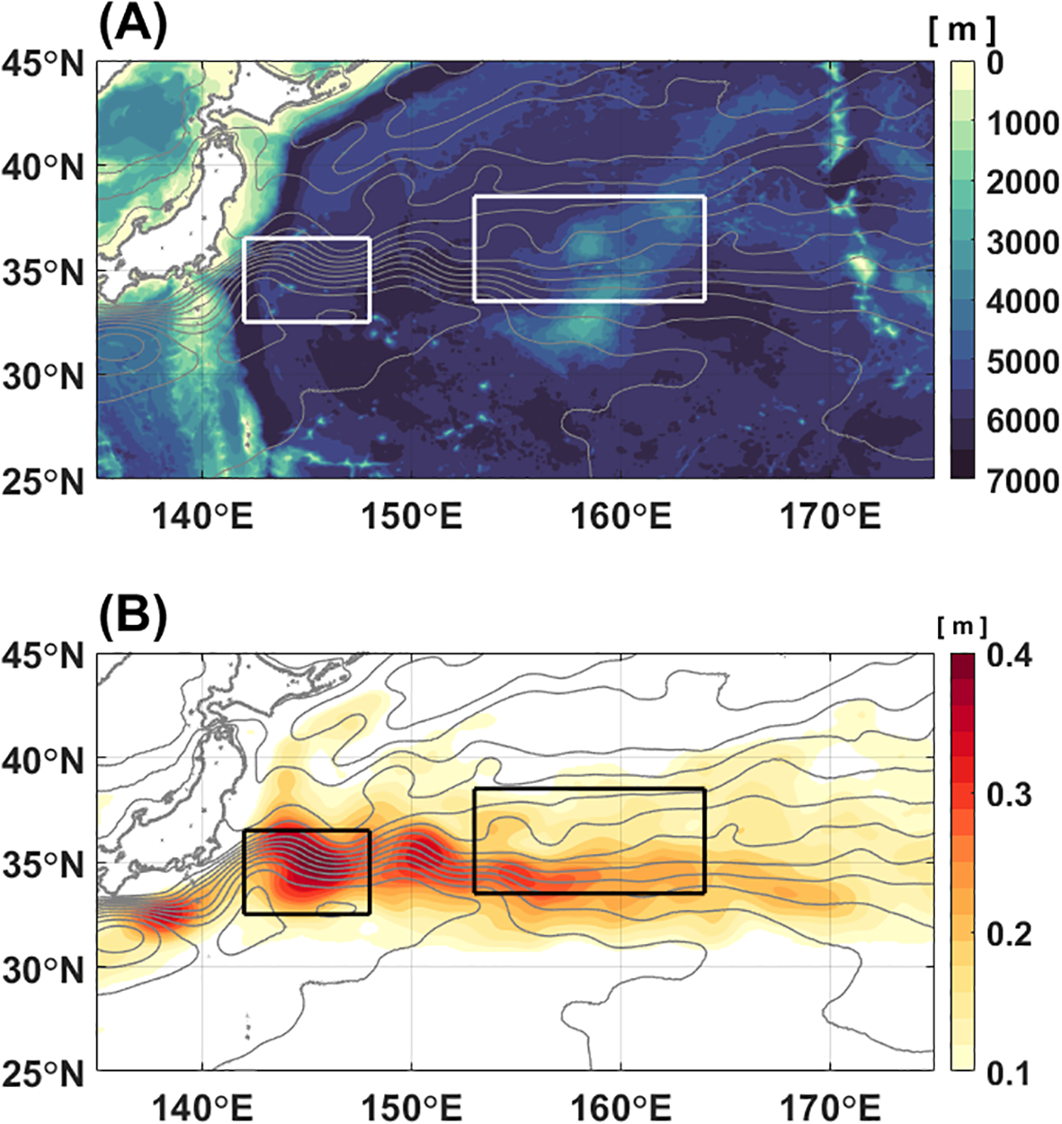
(A) Bathymetry and (B) standard deviation of SSH in the western North Pacific during 1993–2014 derived from FORA-WNP30. Contours denote the mean SSH with an interval of 10 cm. The mean and standard deviation were obtained after applying a 270-day low-pass filter. The upstream (142°–148°E, 32.5°–36.5°N) and downstream (153°–164°E, 33.5°–38.5°N) KE regions used in this study are indicated by rectangular boxes.
Previous studies have revealed that decadal variability of the KE dynamic states is related to atmospheric forcing in the eastern North Pacific (Miller et al., 1998; Deser et al., 1999; Qiu, 2003; Qiu and Chen, 2005, 2010; Andres et al., 2009; Kelly et al., 2010; Kwon et al., 2010; Qiu et al., 2014; Na et al., 2018; Joh and Di Lorenzo, 2019). The negative wind stress curl (WSC) anomalies associated with the negative phase of the Pacific Decadal Oscillation (PDO) or the positive phase of the North Pacific Gyre Oscillation (NPGO) induce positive sea surface height (SSH) anomalies in the subtropical eastern North Pacific. These wind-induced positive SSH anomalies propagate westward into the upstream KE region for 3–4 years as baroclinic Rossby waves and modulate the KE’s dynamic system, including the strengthening of the Kuroshio jet and stabilization of eddy activity (Miller et al., 1998, 2004; Di Lorenzo et al., 2008; Frankignoul et al., 2011; Newman et al., 2016). In turn, the KE is in a stable state (lower EKE) due to the positive SSH anomalies originating from the eastern North Pacific, indicating that downstream variability precedes upstream variability in the KE.
On the other hand, a study by Yang et al. (2018) suggested that the EKE variability in the upstream KE region precedes that in the downstream, exhibiting opposite signs between the upstream (142°–148°E, 32.5°–36.5°N) and downstream KE regions (153°–164°E, 33.5°–38.5°N). They demonstrated that weakening of the upstream KE jet intensifies baroclinic and barotropic instabilities, resulting in meandering of the jet and an increase in the EKE over the upstream region. However, the EKE in the downstream decreases due to the weakening of the KE jet and a decrease in the downstream advection of the EKE. Conversely, a stronger and more stable KE jet suppresses local eddy growth in the upstream region but induces stronger downstream advection of the EKE, indicating that downstream EKE levels are mainly controlled by the dynamics of the upstream KE (Yang et al., 2018).
Although these different sources of EKE variability, upstream-driven and downstream-driven, may appear contradictory, they can be distinguished by distinct temporal scales. For the downstream-driven case, the WSC-induced SSH anomalies over the eastern and central North Pacific propagate westward into the KE upstream region with a multiyear timescale. Meanwhile, for the upstream-driven case, the negative EKE anomalies in the upstream region enhance horizontal advection to the downstream on a shorter timescale of about 300 days (Yang et al., 2018). Since these two distinct processes have been investigated separately, it is necessary to examine whether they occur independently or exhibit some dynamical linkage. Demonstrating a possible linkage between the downstream-driven and the upstream-driven cases could deepen our understanding of the connectivity between the upstream and downstream KE region in terms of the EKE variability.
This study aims to investigate the connectivity of EKE variability between the upstream and downstream KE over timescales ranging from seasonal to decadal. Considering the temporal and spatial scales of the eddy variability in the KE region, a daily high-resolution (~ 1/10°) reanalysis product was utilized. In this study, the upstream KE is defined as 142°–148°E, 32.5°–36.5°N and the downstream KE as 153°–164°E, 33.5°–38.5°N (rectangular boxes in Figure 1), following Yang et al. (2018). Details of the data and methods are described in Section 2. The EKE variability and its characteristics are presented in Section 3. Section 4 provides a conclusion as well as discussions.
2 Data and methods
The Four-dimensional Variational Ocean Reanalysis for the Western North Pacific over 30 years (FORA-WNP30; Usui et al., 2017) was used to examine the EKE variability in the KE region. The FORA employs the four-dimensional variational analysis scheme version of the Multivariate Ocean Variational Estimation system (MOVE-4DVAR; Usui et al., 2015) to assimilate in situ and satellite observations. The horizontal resolution ranges from 1/10° to 1/6°, with 54 vertical levels using a sigma coordinate. In this study, the daily data sets of current velocity and temperature were analyzed from 1993 to 2014 in the upper 700 m for the KE region (130°–175°E, 25°–45°N).
The satellite altimetry data distributed by Copernicus Marine Service (https://marine.copernicus.eu/) was also analyzed and compared with the FORA. The gridded sea level anomalies are produced with a horizontal resolution of 1/4° by merging the measurements from multiple missions. The geostrophic current velocity from the daily absolute dynamic topography were used to calculate the EKE from 1993 to 2023.
The EKE was calculated as:
where the and represent the deviation of the zonal and meridional current velocity from their 270-day running mean values (Yang et al., 2018). To examine the EKE variability on seasonal to decadal time scales, a 270-day low-pass filter was further applied to the calculated EKE. “EKE” hereafter refers to the low-pass filtered time series. Changing the low-pass cutoff to either 180 or 365 days does not qualitatively affect the results.
The EKE index was calculated for the upstream region (EKE Index-UP; 142°–148°E, 32.5°–36.5°N) and for the downstream region (EKE Index-DN; 153°–164°E, 33.5°–38.5°N) as the spatially-averaged and normalized time series of the EKE, following Yang et al. (2018). The four dynamic states of the KE were also defined as follows: 1) “upU+downU”; larger EKE in both the upstream and downstream (EKE Index-UP > +1 and Index-DN > +1; both unstable), 2) “upU+downS”; larger EKE in the upstream (EKE Index-UP > +1; unstable) but smaller in the downstream (Index-DN < –1; stable), 3) “upS+downU”; smaller EKE in the upstream (EKE Index-UP < –1; stable) but larger in the downstream (Index-DN > +1; unstable), and 4) “upS+downS”; smaller EKE in both the upstream and downstream (EKE Index-UP < –1 and Index-DN < –1; both stable). The definitions of the four KE dynamic states are also presented in Table 1.
Table 1
| Dynamic state | Definition |
|---|---|
| upU+downU | EKE Index-UP > +1 and Index-DN > +1 |
| upU+downS | EKE Index-UP > +1 and Index-DN < –1 |
| upS+downU | EKE Index-UP < –1 and Index-DN > +1 |
| upS+downS | EKE Index-UP < –1 and Index-DN < –1 |
Definitions of KE dynamic states based on the upstream (UP) and downstream (DN) EKE indices.
Note that the EKE indices are calculated from spatially averaged and normalized time series of EKE.
To diagnose the eddy energy flux, the divergence induced by the advection process was examined using the following equation:
where are velocity anomalies used in equation (1), and the symbol ∇ represents the two-dimensional gradient operator. In addition, the empirical orthogonal function (EOF) technique was applied to extract dominant modes of the EKE variability in the entire KE region, including both upstream and downstream.
The sea level pressure (SLP) and 10-m wind speed were obtained from the European Centre for Medium-Range Weather Forecasts (ECMWF) Reanalysis-5 (ERA-5; https://cds.climate.copernicus.eu/; Hersbach et al., 2020). The monthly atmospheric variables with a horizontal resolution of 1/4° were analyzed for a longer period from 1990 to 2017 in order to understand the lead-lag relationship between the EKE and atmospheric variability. The 270-day (or 9-month) low-pass filtering was applied to all the oceanic and atmospheric variables used in this study to focus on their long-term (seasonal to decadal) variability.
3 Results
Figure 2 shows the mean and standard deviation of the EKE based on FORA and satellite altimetry during 1993–2014. The EKE from FORA generally exhibits a larger mean and standard deviation over an extended region compared to those from satellite altimetry, not only due to FORA’s higher spatial and temporal resolution, but also because of its model biases. However, both FORA and satellite altimetry show a large mean and standard deviation of EKE along the KE jet at 33°–36°N. The higher EKE along the KE jet is attributed to the meandering of the KE jet and the energetic pinch-off of eddies from the jet (Qiu and Chen, 2005, 2010; Qiu et al., 2014; Yang et al., 2018; Wang and Pierini, 2020). The mean and standard deviation decrease to the east of ~155°E, as the KE jet becomes broader and slower. All the following results use the EKE based on FORA.
Figure 2
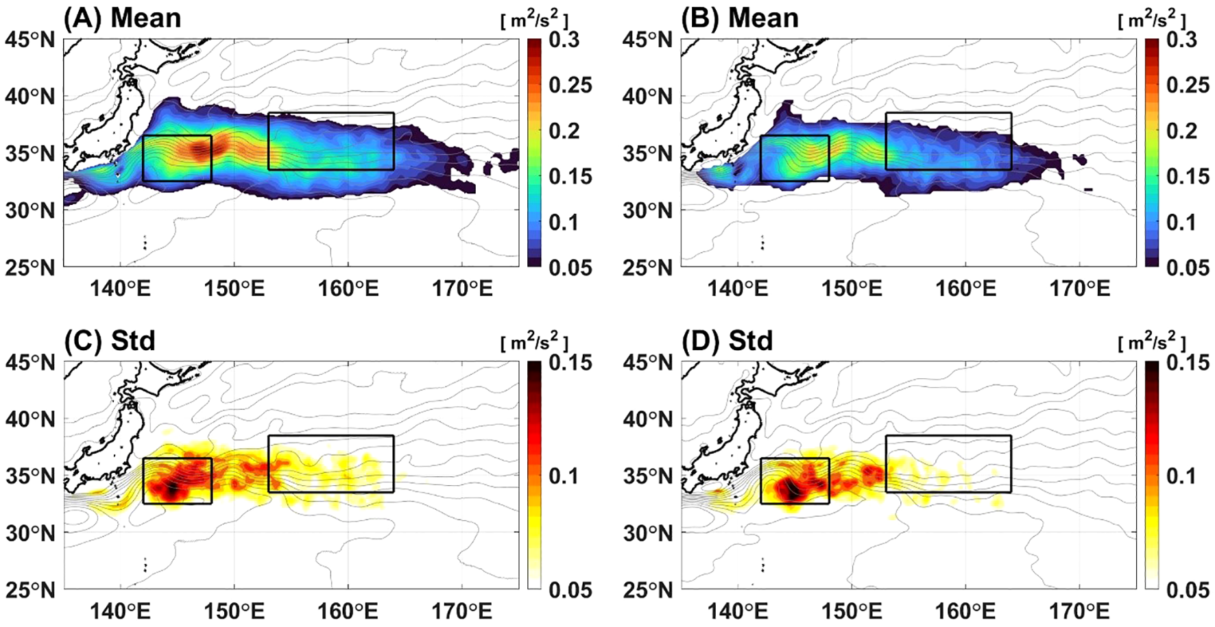
The (A) mean and (C) standard deviation of EKE during 1993–2014 derived from FORA-WNP30. (B, D) are the same as (A, C), respectively, but are derived from satellite altimetry. Contours denote the mean SSH of each dataset with an interval of 10 cm. The mean and standard deviation were obtained from a 270-day low-pass filtered EKE, as defined in equation (1).
Figure 3 presents the spatially-averaged and normalized EKE time series in the upstream and downstream regions (EKE Index-UP and EKE Index-DN). Both the upstream and downstream EKE exhibit pronounced decadal-scale fluctuations, possibly reflecting the influence of PDO and NPGO (Qiu and Chen, 2005, 2010; Andres et al., 2009; Kwon et al., 2010; Qiu et al., 2014; Na et al., 2018; Joh and Di Lorenzo, 2019). Notably, the strong negative correlation is found between the upstream and downstream EKE. At lag 0, the correlation is -0.31, which increases in magnitude to -0.54 when the upstream leads the downstream by 230 days. In other words, both upstream and downstream EKE vary on decadal timescales and are negatively correlated.
Figure 3
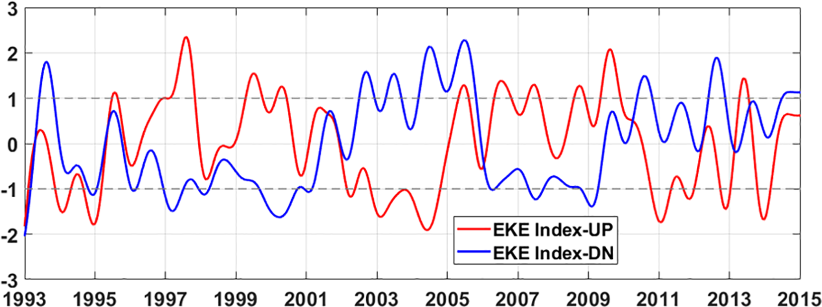
Time series of the EKE Index-UP (red; upstream; 142°–148°E, 32.5°–36.5°N) and EKE Index-DN (blue; downstream; 153°–164°E, 33.5°–38.5°N) derived from FORA-WNP30. The EKE indices were obtained from spatially averaged and normalized time series of the EKE for the KE upstream and downstream regions, respectively.
Although the negative relationship between upstream and downstream EKE, as reported by Yang et al. (2018), implies that a strengthening of EKE in one region tends to coincide with a weakening of EKE in the other region, there were instances when both upstream and downstream EKE strengthened (e.g., mid-2005) or weakened at the same time (e.g., winter 1994/1995). Accordingly, a composite analysis was conducted based on the EKE Index-UP and EKE Index-DN to investigate the spatial distribution of EKE under the different dynamic states (Table 1). According to the definition, 140 days were categorized as “upU+downU”, 369 days as “upU+downS”, 458 days as “upS+downU”, and 130 days as “upS+downS” states. Figure 4 shows the composites of the EKE for the four dynamic states. It can be expected that the upU+downU state shows a high EKE, and the “upS+downS” state shows a low EKE all over the KE region. During the “upU+downS state”, the EKE levels are pronounced in the upstream region, with large amplitudes confined to the west of 170°E. In contrast, although the “upS+downU” state generally exhibits weaker EKE compared to the “upU+downS” state, the region with EKE higher than 0.05 m2/s2 extends farther eastward beyond 170°E.
Figure 4
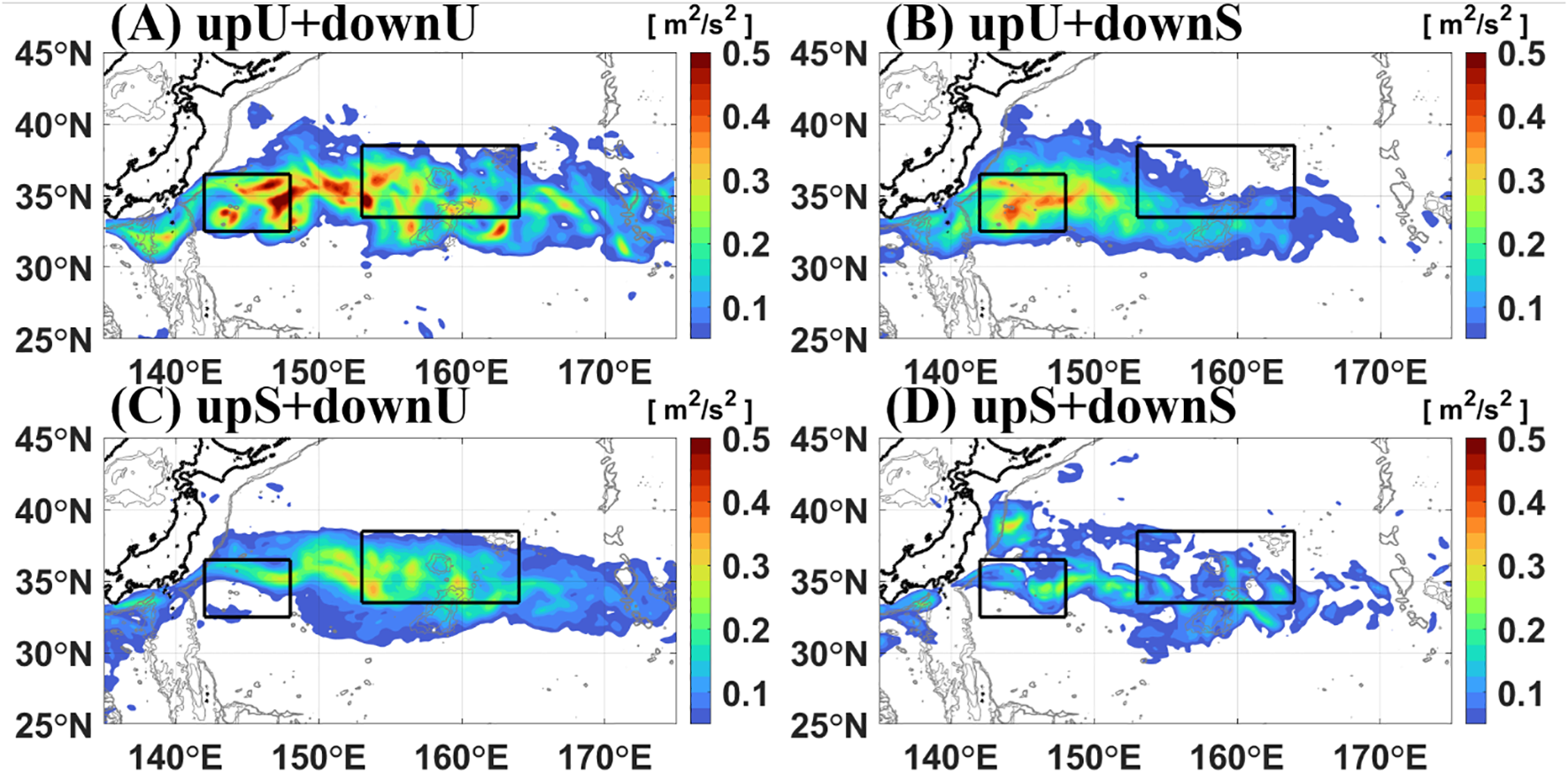
Composites of EKE for the four KE dynamic states: (A) “upU+downU” (EKE Index-UP > +1, Index-DN > +1), (B) “upU+downS” (EKE Index-UP > +1, Index-DN < –1), (C) “upS+downU” (EKE Index-UP < –1, Index-DN > +1), and (D) “upS+downS” (EKE Index-UP < –1, Index-DN < –1). The black boxes indicate the upstream and downstream KE regions.
To diagnose the conditions of KE jet associated with the four dynamic states based on the EKE indices, the anomalies of the upper 700 m depth-averaged temperature and 0.5 m current velocity are shown in Figure 5. During the “upU+downU” state, both warm and cold anomalies are observed in the upstream and downstream regions, with signatures of strong meandering and mesoscale eddies (Figure 5A; Mizuno and White, 1983; Yang et al., 2018). However, cold anomalies are observed to the south of the KE jet at approximately 35°N during the “upU+downS” state, while warm anomalies are observed during the “upS+downU” state (Figures 5B, C). The cold anomalies to the south contribute to weakening the jet and its recirculation gyre, while the warm anomalies contribute to strengthening the jet associated with the meridional gradient of temperature. This result is consistent with previous studies that have shown that when the KE jet and its recirculation gyre are in a weak state, higher EKE and lower SSH are observed compared to the stable state with a stronger KE jet (Qiu and Chen, 2005, 2010). In comparison to the “upU+downS” and “upS+downU” states, the “upS+downS” state exhibits colder temperature anomalies in the upstream region (Figure 5D), which would typically be associated with negative SSH anomalies and increased EKE. However, this state exhibits lower EKE levels (Figure 4D), which does not fully align with the previous studies.
Figure 5
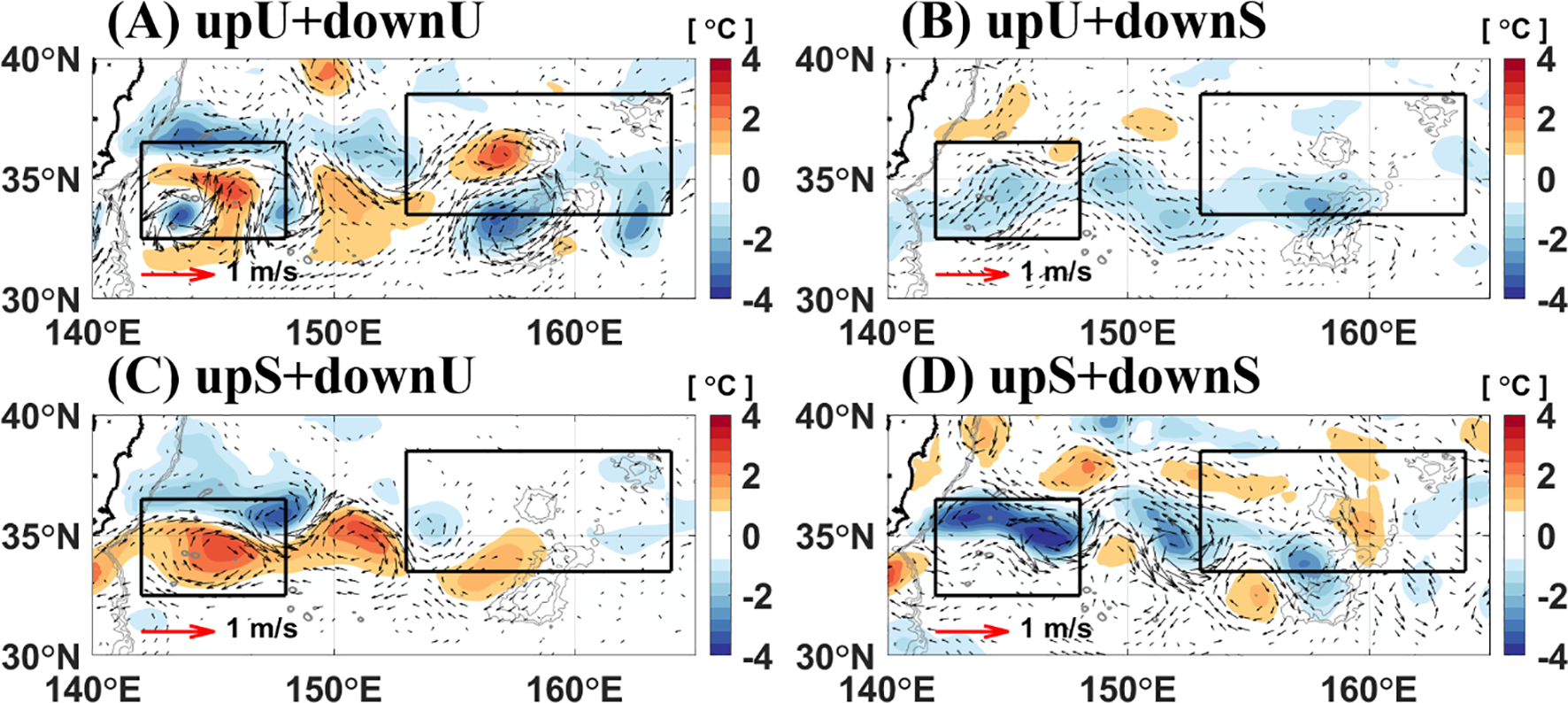
Composites of the upper 700-m depth-averaged temperature and 0.5-m current velocity anomalies for the four KE dynamic states: (A) “upU+downU” (EKE Index-UP > +1, Index-DN > +1), (B) “upU+downS” (EKE Index-UP > +1, Index-DN < –1), (C) “upS+downU” (EKE Index-UP < –1, Index-DN > +1), and (D) “upS+downS” (EKE Index-UP < –1, Index-DN < –1). The black boxes indicate the upstream and downstream KE regions.
Figure 6A compares the four dynamic states based on the latitudinal axis of the KE jet, determined by the location of the maximum meridional gradient of SSH. The axis is most variable during the “upU+downU” state, both upstream and downstream (highlighted in red in Figure 6A). Interestingly, although the “upS+downS” state is generally considered stable, the latitudinal axis of the KE jet also exhibits significant fluctuations in the downstream region (indicated in blue in Figure 6A). Figure 6B presents the meridional gradient of the SSH at the latitude defined as an axis in Figure 6A, indicating the strength of the jet. The KE jet is strongest both upstream and downstream during the upS+downU state (light blue in Figure 6B), not during the “upS+downS” state (blue in Figure 6B). This implies that the dynamical link between the northward shift and stronger jet during the stable state (Qiu and Chen, 2005; Qiu et al., 2014) may not apply to the downstream KE region.
Figure 6
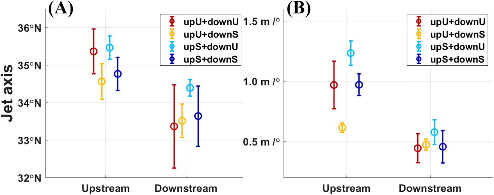
(A) The averaged latitudinal position of the KE jet and (B) the magnitude of the SSH gradient along the KE jet in the upstream and downstream regions during the four dynamic states. The vertical bars denote the standard deviations.
In order to understand the complex relationship of the EKE variability between the upstream and downstream KE regions, the EOF analysis was performed, including both regions. The first EOF mode explains approximately 30% of the total variance (Figure 7). The spatial pattern exhibits a dipole characteristic to the west and east of ~150°E, with the largest amplitude located at approximately 145°E and 34°N, to the south of the mean latitude of the KE jet. The first EOF mode is consistent with that from the EKE based on satellite altimetry both in terms of the spatial patterns and the principal component (PC) time series (correlation: 0.96; not shown). It is remarkable that the PC time series of the first mode is highly correlated with the EKE Index-UP (correlation: 0.90; black and red lines in Figure 7B), indicating that the EKE variability in the KE region is dominated by its upstream variability. Thus, the first mode exhibits an out-of-phase relationship between the upstream and downstream, particularly on a decadal time scale. This out-of-phase relationship between the upstream and downstream is consistent with the results reported by Yang et al. (2018). However, the negative anomalies in the downstream region appear to be more spatially extensive, spanning from 150°E to 175°E, compared to those reported by Yang et al. (2018). This broader zonal extent may reflect differences in temporal and spatial resolution of the dataset.
Figure 7
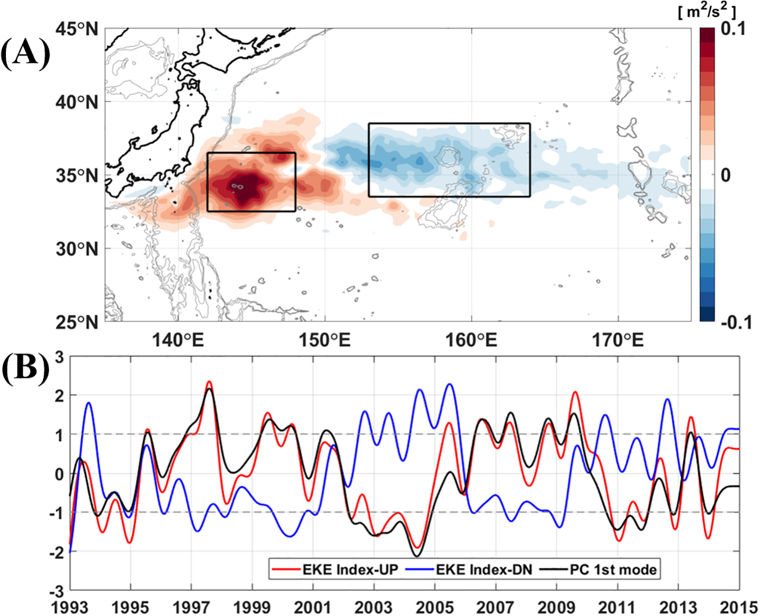
(A) Spatial pattern of the first EOF mode of EKE during 1993–2014 derived from FORA-WNP30. (B) Time series of EKE Index-UP (red), EKE Index-DN (blue), and the PC-1 time series (black). The black boxes in (A) denote the areas used to represent the upstream and downstream regions.
Figure 8 shows the first three EOF modes of the EKE variability in the KE region. Unlike the first mode, the second mode shows an in-phase spatial pattern between the upstream and downstream regions, and the PC time series exhibits strong seasonal variability with an interannual modulation, characterized by a maximum from June to September and a minimum from December to March. Wang and Pierini (2020) revealed that the EKE reaches its maximum in summer when the KE is in a stable state, while it peaks in autumn when the KE is in an unstable state. They found that the processes of baroclinic energy transfer related to the zonal (meridional) density gradients are the main factors in modulating the seasonal variation in the EKE for the stable (unstable) state. Although the EOF analysis was performed without considering the KE dynamic states in this study, the second mode exhibits higher EKE in summer and lower EKE in winter, which is consistent with previous studies (Wang and Pierini, 2020; Yang and Liang, 2018; Yang et al., 2023).
Figure 8
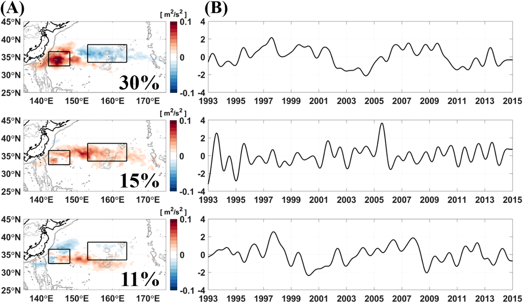
(A) The spatial patterns of the first three EOF modes and (B) their corresponding PC time series (from top to bottom). The percentage of variance explained by each mode is displayed in each panel in (A). The black boxes in (A) denote the areas used to represent the upstream and downstream regions.
The third mode exhibits positive anomalies in the eastern part of the upstream KE region, and its PC time series is correlated with that of the first mode when the third mode precedes the first mode with a time lag of two years (correlation: 0.53). This lagged relationship suggests that the positive EKE anomalies south of the downstream region associated with the third mode may contribute to the development of positive anomalies in the upstream region associated with the first mode after two years. The three EOF modes mostly explain the EKE variability in the KE region and modulate the relationship between upstream and downstream EKE variability.
4 Conclusion and discussions
This study investigated the EKE variability in the KE region by applying EOF analysis to the high-resolution ocean reanalysis, FORA, with a focus on the connectivity between its upstream and downstream variability. It was found that this connectivity occurs on multiple time scales. Seasonal-scale variability emerges as the second EOF mode, whose pattern reflects the strengthening and weakening of eddy activity across the entire KE system, including both upstream and downstream regions. Specifically, EKE tends to be enhanced in summer and suppressed in winter, modulated by interannual variability. In comparison, the decadal-scale variability is depicted as two separate modes, the first and third EOF modes. The spatial pattern of the first mode exhibits a dipole pattern with opposite signs between the upstream and downstream regions. The PC time series of the third EOF mode (PC-3) leads that of the first mode (PC-1) by about two years with a positive correlation. Notably, the spatial pattern of the third EOF mode extends zonally eastward from the upstream. The time-lag relationship between PC-1 and PC-3, together with their spatial patterns, suggests that a common process may be captured by two different modes depending on its temporal evolution.
Figure 9 shows that the out-of-phase relationship between the upstream and downstream EKE variability is linked to the NPGO index with distinct time lags. The NPGO index precedes the PC-3 by 10 months, and the PC-3 leads the PC-1 by 24 months. Considering these lead-lag relationships, the PC-1 and NPGO index (solid black and green lines in Figure 9) are shifted relative to PC-3, which serves as the reference time series. These lead–lag relationships are quantitatively summarized in Table 2, which lists the maximum correlation coefficients, the corresponding time lags, and the effective degrees of freedom (EDOF). Table 2 shows that the NPGO leads PC-3 by 10 months, PC-3 leads PC-1 by 23–24 months, and the NPGO leads PC-1 by about 30 months; all are significant at the 95% confidence level. The NPGO index and PC-1 show the strongest correlation when the NPGO index leads the PC-1 by approximately 30 months (correlation: -0.64). According to previous studies, the negative phase of the NPGO is linked to atmospheric forcing that induces negative SSH anomalies in the central and eastern North Pacific. These anomalies propagate westward into the KE region via baroclinic Rossby waves over ~3 years. The significant relationship with the NPGO index, particularly on the decadal time scale, suggests that the atmospheric forcing in the eastern North Pacific may be responsible for the first and third modes of the EKE variability in the KE region. In contrast, the correlation between the PDO and PC-3 is not statistically significant. However, the PDO shows a significant correlation with PC-1 (correlation: 0.57) with a time lag of approximately 40 months. Based on the correlations among PC-1, PC-3, the NPGO index, and the PDO index, decadal variability of the EKE in the KE region appears to be more closely linked to the NPGO than to the PDO. The correlation between the NPGO and KE EKE is -0.59 during 1993–2014 but becomes insignificant when the analysis period is extended to 1993–2023 based on satellite altimetry data. This weakening is likely associated with the large meander of the Kuroshio in 2017 (Wang and Pierini, 2023), which constrained the Kuroshio path to the northern deep channel of the Izu Ridge and sustained positive SSH anomalies in the upstream region (Qiu et al., 2020). Under such conditions, the westward propagation of NPGO-related SSH anomalies was suppressed, leading to a stable KE state that was no longer directly modulated by the NPGO. This regime-dependent linkage highlights that the influence of the NPGO on KE variability is not stationary but can be interrupted by a persistent large meander of the Kuroshio.
Figure 9
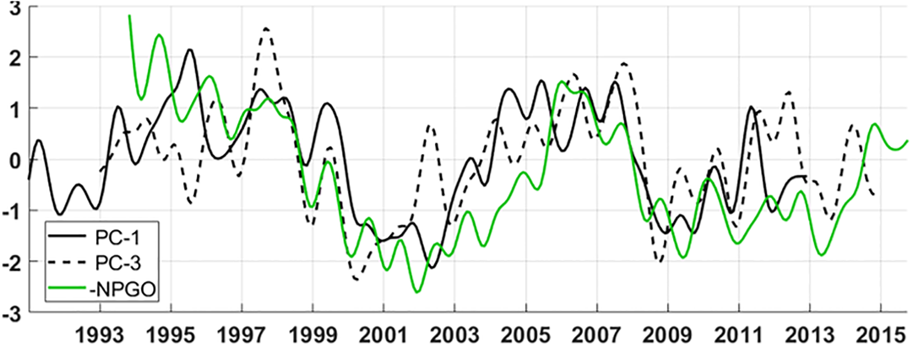
Time series of the first (PC-1, solid black) and third (PC-3, dashed black) EOF modes of the EKE, along with the North Pacific Gyre Oscillation (NPGO) index (green). The time axis is referenced to the PC-3 time series. Based on the lead-lag relationship, PC-1 is shifted forward by 24 months, and the NPGO index is shifted backward by 10 months. Note that the NPGO index is plotted with its sign inverted after applying a 9-month low-pass filter.
Table 2
| PC-1 & PC-3 | NPGO | PDO | ||
|---|---|---|---|---|
| r (lag) (EDOF) |
PC-1 | 0.54* (PC-3 leads by 23 m) (15) |
-0.64* (30 m) (10) |
0.57* (42 m) (20) |
| PC-3 | -0.56* (10 m) (16) |
0.39 (3 m) (28) |
Lag correlations of PC-1 and PC-3, and their correlations with the NPGO and PDO indices, obtained after applying a 270-day (9-month) low-pass filter.
The values shown are the maximum correlation coefficient (r), the corresponding time lag (lag, in months), and the effective degrees of freedom (EDOF) accounting for autocorrelation. Positive lags indicate that NPGO or PDO precedes the PC time series of EKE.*Significant at the 95% confidence level based on t-test.
To further examine whether these processes are reflected in the first and third modes, the SLP and WSC anomalies are plotted at a lag of 30 months, when the correlation between the NPGO and PC-1 was maximized (Figure 10). A negative SLP anomaly in the central–eastern North Pacific and a positive SLP anomaly in the Bering Sea (160°E–160°W, 55°N–65°N) represent the North Pacific Oscillation, which serves as the atmospheric expression of the NPGO (Di Lorenzo et al., 2008; Ceballos et al., 2009). The positive WSC anomaly accompanying the negative SLP anomaly leads to negative SSH anomalies in the central Pacific (Figure 11A). These anomalies propagate westward over ~30 months into the upstream KE region. Their propagation speed is estimated to be about 5.0 cm/s, which is similar to the speed of the first baroclinic Rossby wave at these latitudes (Chelton et al., 2011). As negative SSH anomalies, initially formed in the central Pacific, propagate toward the KE region, they develop a narrower meridional structure, explained by “thin-jet” theory (Sasaki and Schneider, 2011; Sasaki et al., 2013), in which Rossby waves are guided and trapped by the sharp KE front. Since the KE jet axis is located near 35°N, a negative SSH anomaly south of this latitude weakens the KE jet, as shown in Figure 5B. A weakened KE jet tends to lead to an unstable KE path, thereby enhancing eddy activity (Figure 11; Qiu and Chen, 2005, 2010). Meanwhile, a positive EKE anomaly is observed overlapping with the westward propagating negative SSH anomaly (Figure 11B). When the Rossby wave begins to influence the downstream region at a lag of 24 months, a zonally elongated positive EKE anomaly appears alongside the negative SSH anomaly (Figure 11). The resemblance of this pattern to the third EOF mode, together with the two-year lag between PC-1 and PC-3, suggests that the KE system responds to remote Rossby waves, resulting in the delayed relationship between the first and third EOF modes.
Figure 10
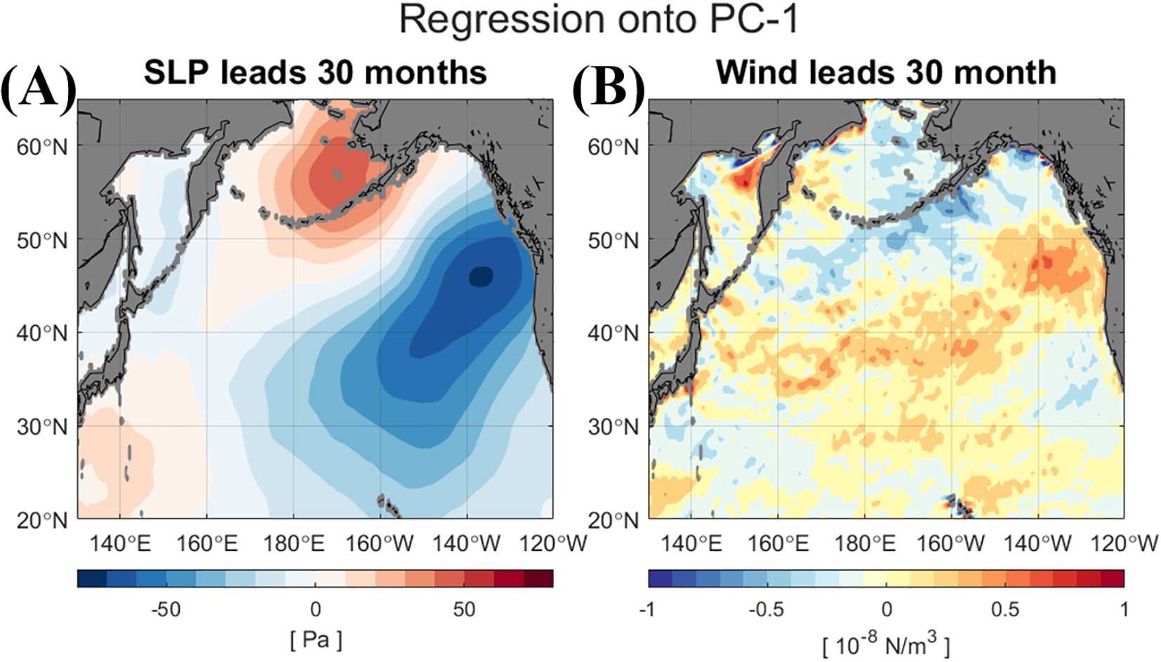
Regression maps of (A) sea level pressure (SLP) and (B) wind stress curl (WSC) onto PC-1, with a lag of 30 months. This lag corresponds to the time at which the NPGO index leads PC-1 with the strongest correlation, indicating that NPGO-related variability precedes that of PC-1 by approximately 30 months. The regression coefficients of SLP and WSC were calculated after removing their seasonal cycles.
Figure 11
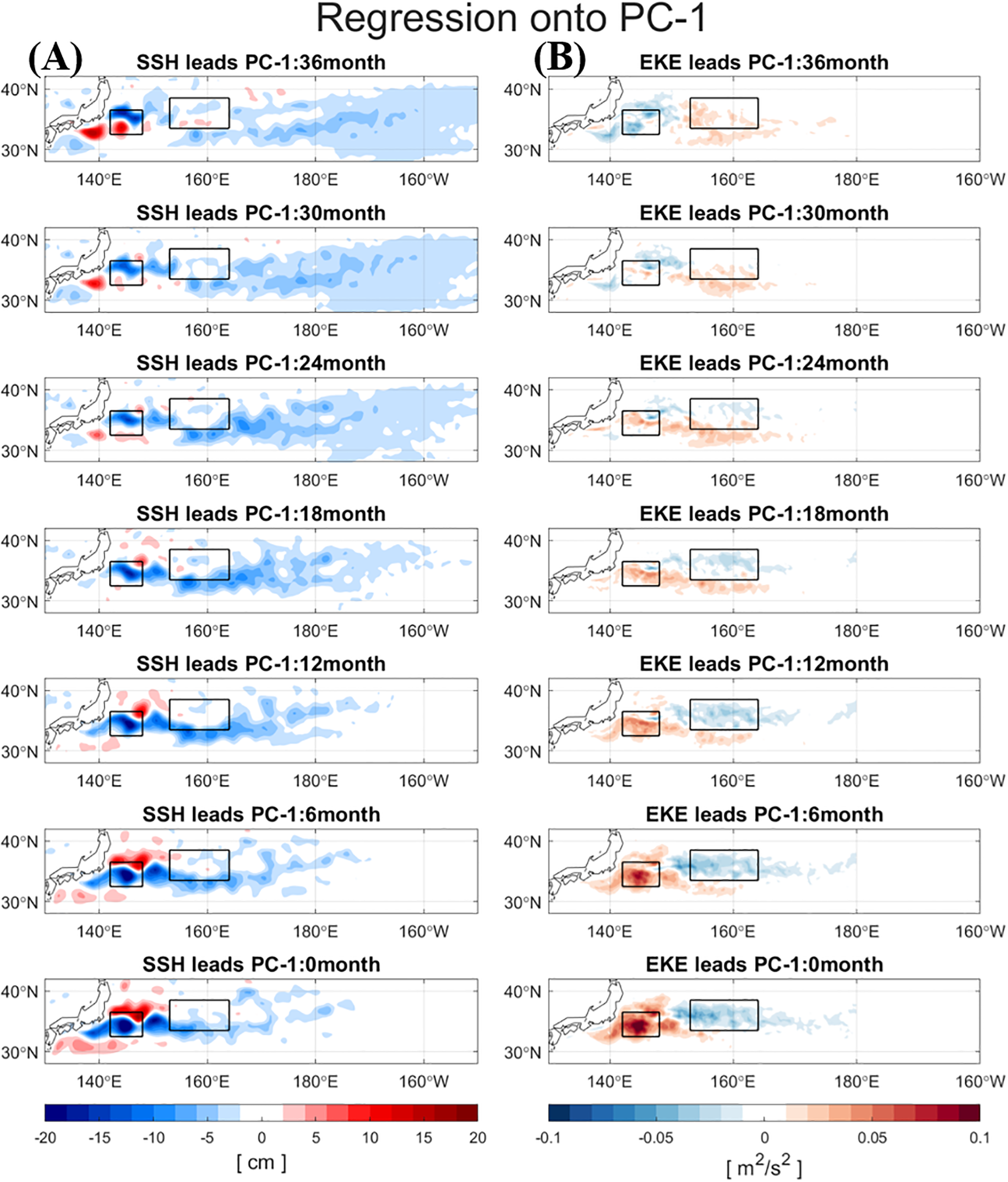
Lead–lag regression maps of (A) SSH and (B) EKE onto the PC-1 with time lags ranging from 36 to 0 months (top to bottom) at 6-month intervals. Positive lags indicate that SSH or EKE leads the PC-1. The regression coefficients of SSH and EKE were calculated after removing their seasonal cycles.
It may seem contradictory to Yang et al. (2018), who showed that a weakened upstream KE jet could contribute to a downstream reduction in EKE, dominated by the advective process. To investigate the dynamical linkage between downstream-driven and upstream-driven variability, the EKE advection term was calculated based on equation (2) and regressed onto PC-1. Figure 12 shows the spatially integrated EKE advection values over the upstream and downstream regions. A positive value indicates a gain of EKE through advection. Indeed, starting from approximately 24 months, when the negative SSH anomaly begins to affect the downstream region, positive (negative) EKE advection in the upstream (downstream) region is observed (Figure 12). The advection of anomalies persists for several months, reaching a peak approximately 6 months before the EKE dipole pattern fully develops. Following the peak in EKE advection, the anomalies in both the upstream and downstream regions appear to weaken. However, the negative anomaly in the downstream region intensifies again, which provides a favorable condition for a reduction in EKE. It may help explain why the positive EKE anomaly in the upstream region leads the negative anomaly in the downstream region by 230 days.
Figure 12
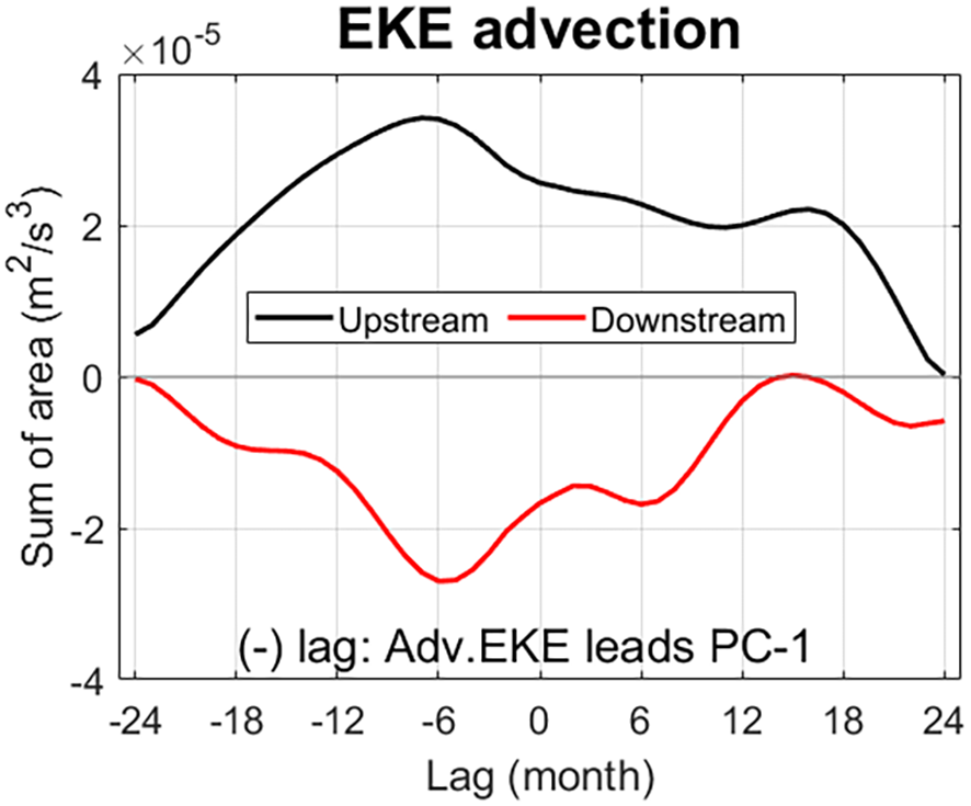
Time series of the lead–lag regression of EKE advection onto the PC-1, ranging from -24 to +24 months. The EKE advection values—where positive values indicate a gain of EKE through advection—were spatially integrated within the upstream (black) and downstream regions (red), based on regression coefficients at each lag. Negative lags indicate that PC-1 leads the EKE advection. The EKE advection is calculated based on equation (2).
Wang and Pierini (2023) proposed that eddy activity in the Kuroshio large meander (KLM) region modulates upstream EKE between 33–37°N and 142–146°E through an advective process, but they found no significant link to downstream EKE variability. This study demonstrates that the relationship of eddy activity between the upstream and downstream regions of the KE occurs on distinct spatial and temporal scales. This finding contributes to an in-depth understanding of how remote influences affect the KE jet via the downstream region, with the KE jet subsequently feeding back into the downstream region. This understanding of upstream–downstream connectivity could provide a basis for enhancing the predictability of KE states on seasonal to decadal timescales. However, the process of eddy energetics needs to be investigated more quantitatively using an eddy-resolving model with higher spatial resolution that accounts for the slower KE jet in the downstream region. Furthermore, the role of air-sea interactions, such as buoyancy forcing (Ma et al., 2016), heat flux exchange (Yang et al., 2019), and current-wind feedback (Shan et al., 2020), may also need to be considered to fully understand the redistribution process of EKE. Further investigation is required in future studies to explore how these air-sea interactions impact the KE dynamic states and advective processes in the downstream region, utilizing high-resolution coupled models.
Statements
Data availability statement
The original contributions presented in the study are included in the article/supplementary material. Further inquiries can be directed to the corresponding author.
Author contributions
SL: Formal Analysis, Visualization, Writing – original draft, Validation, Data curation, Writing – review & editing, Investigation, Methodology. HN: Supervision, Writing – review & editing, Writing – original draft, Funding acquisition, Resources, Project administration, Conceptualization. Y-GP: Writing – original draft, Resources, Conceptualization, Funding acquisition, Project administration, Supervision, Writing – review & editing. H-JP: Validation, Writing – review & editing, Methodology, Formal Analysis, Writing – original draft, Visualization. SC: Validation, Writing – original draft, Writing – review & editing.
Funding
The author(s) declare that financial support was received for the research and/or publication of this article. This research was supported by the National Research Foundation funded by the Ministry of Science and ICT (2022M3I6A1085990), and the Korea Institute of Marine Science & Technology (KIMST) funded by the Ministry of Oceans and Fisheries (RS-2023-00256330, under the “Development of risk managing technology tackling ocean and fisheries crisis around Korean Peninsula by Kuroshio Current” project, and RS-2025-02217872), Korea.
Conflict of interest
The authors declare that the research was conducted in the absence of any commercial or financial relationships that could be construed as a potential conflict of interest.
Generative AI statement
The author(s) declare that no Generative AI was used in the creation of this manuscript.
Any alternative text (alt text) provided alongside figures in this article has been generated by Frontiers with the support of artificial intelligence and reasonable efforts have been made to ensure accuracy, including review by the authors wherever possible. If you identify any issues, please contact us.
Publisher’s note
All claims expressed in this article are solely those of the authors and do not necessarily represent those of their affiliated organizations, or those of the publisher, the editors and the reviewers. Any product that may be evaluated in this article, or claim that may be made by its manufacturer, is not guaranteed or endorsed by the publisher.
References
1
Andres M. Park J. H. Wimbush M. Zhu X. H. Nakamura H. Kim K. et al . (2009). Manifestation of the Pacific decadal oscillation in the Kuroshio. Geophys. Res. Lett.36. doi: 10.1029/2009GL039216
2
Ceballos L. I. Di Lorenzo E. Hoyos C. D. Schneider N. Taguchi B. (2009). North Pacific Gyre Oscillation synchronizes climate fluctuations in the eastern and western boundary systems. J. Clim.22, 5163–5174. doi: 10.1175/2009JCLI2848.1
3
Chelton D. B. Schlax M. G. Samelson R. M. (2011). Global observations of nonlinear mesoscale eddies. Prog. Oceanogr.91, 167–216. doi: 10.1016/j.pocean.2011.01.002
4
Deser C. Alexander M. A. Timlin M. S. (1999). Evidence for a wind-driven intensification of the Kuroshio Current Extension from the 1970s to the 1980s. J. Clim.12, 1697–1706. doi: 10.1175/1520-0442(1999)012<1697:EFAWDI>2.0.CO;2
5
Di Lorenzo E. Schneider N. Cobb K. M. Franks P. Chhak K. Miller A. J. et al . (2008). North Pacific Gyre Oscillation links ocean climate and ecosystem change. Geophys. Res. Lett.35. doi: 10.1029/2007GL032838
6
Frankignoul C. Sennéchael N. Kwon Y. O. Alexander M. A. (2011). Influence of the meridional shifts of the Kuroshio and the Oyashio Extensions on the atmospheric circulation. J. Clim.24, 762–777. doi: 10.1175/2010JCLI3731.1
7
Hersbach H. Bell B. Berrisford. P. Hirahara S. Horányi A. Muñoz-Sabater J. et al . (2020). The ERA5 global reanalysis. Q J. R Meteorol Soc146, 1999–2049. doi: 10.1002/qj.3803
8
Joh Y. Di Lorenzo E. (2019). Interactions between Kuroshio Extension and Central Tropical Pacific lead to preferred decadal-timescale oscillations in Pacific climate. Sci. Rep.9, 13558. doi: 10.1038/s41598-019-49927-y
9
Kelly K. A. Small R. J. Samelson R. M. Qiu B. Joyce T. M. Kwon Y. O. et al . (2010). Western boundary currents and frontal air–sea interaction: gulf stream and kuroshio extension. J. Clim.23, 5644–5667. doi: 10.1175/2010JCLI3346.1
10
Kwon Y. O. Alexander M. A. Bond N. A. Frankignoul C. Nakamura H. Qiu B. et al . (2010). Role of the Gulf Stream and Kuroshio–Oyashio systems in large-scale atmosphere–ocean interaction: A review. J. Clim.23, 3249–3281. doi: 10.1175/2010JCLI3343.1
11
Ma X. Jing Z. Chang P. Liu X. Montuoro R. Small R. J. et al . (2016). Western boundary currents regulated by interaction between ocean eddies and the atmosphere. Nature535, 533–537. doi: 10.1038/nature18640
12
Miller A. J. Cayan D. R. White W. B. (1998). A westward-intensified decadal change in the North Pacific thermocline and gyre-scale circulation. J. Clim.11, 3112–3127. doi: 10.1175/1520-0442(1998)011<3112:AWIDCI>2.0.CO;2
13
Miller A. J. Chai F. Chiba S. Moisan J. R. Neilson D. J. (2004). Decadal-scale climate and ecosystem interactions in the North Pacific Ocean. J. Oceanogr.60, 163–188. doi: 10.1023/b:joce.0000038325.36306.95
14
Mizuno K. White W. B. (1983). Annual and interannual variability in the Kuroshio current system. J. Phys. Oceanogr.13, 1847–1867. doi: 10.1175/1520-0485(1983)013<1847:AAIVIT>2.0.CO;2
15
Na H. Kim K. Y. Minobe S. Sasaki Y. N. (2018). Interannual to decadal variability of the upper-ocean heat content in the western North Pacific and its relationship to oceanic and atmospheric variability. J. Clim.31, 5107–5125. doi: 10.1175/JCLI-D-17-0506.1
16
Newman M. Alexander M. A. Ault T. R. Cobb K. M. Deser C. Di Lorenzo E. et al . (2016). The Pacific decadal oscillation, revisited. J. Climate.29, 4399–4427. doi: 10.1175/JCLI-D-15-0508.1
17
Qiu B. (2003). Kuroshio extension variability and forcing of the pacific decadal oscillations: responses and potential feedback. J. Phys. Oceanogr.33, 2465–2482. doi: 10.1175/1520-0485(2003)033<2465:KEVAFO>2.0.CO;2
18
Qiu B. Chen S. (2005). Variability of the Kuroshio Extension jet, recirculation gyre, and mesoscale eddies on decadal time scales. J. Phys. Oceanogr.35, 2090–2103. doi: 10.1175/JPO2807.1
19
Qiu B. Chen S. (2010). Eddy-mean flow interaction in the decadally modulating Kuroshio Extension system. Deep Sea Res. Part II57, 1098–1110. doi: 10.1016/j.dsr2.2008.11.036
20
Qiu B. Chen S. Schneider N. Oka E. Sugimoto S. (2020). On the reset of the wind-forced decadal Kuroshio Extension variability in late 2017. J. Climate.33, 10813–10828. doi: 10.1175/JCLI-D-20-0237.1
21
Qiu B. Chen S. Schneider N. Taguchi B. (2014). A coupled decadal prediction of the dynamic state of the Kuroshio Extension system. J. Clim.27, 1751–1764. doi: 10.1175/JCLI-D-13-00318.1
22
Sasaki Y. N. Minobe S. (2015). Climatological mean features and interannual to decadal variability of ring formations in the Kuroshio Extension region. J. Oceanogr.71, 499–509. doi: 10.1007/s10872-014-0270-4
23
Sasaki Y. N. Minobe S. Schneider N. (2013). Decadal response of the Kuroshio Extension jet to Rossby waves: Observation and thin-jet theory. J. Phys. Oceanogr.43, 442–456. doi: 10.1175/JPO-D-12-096.1
24
Sasaki Y. N. Schneider N. (2011). Decadal shifts of the kuroshio extension jet: application of thin-jet theory. J. Phys. Oceanogr.41, 979–993. doi: 10.1175/2011JPO4550.1
25
Shan X. Jing Z. Sun B. Wu L. (2020). Impacts of ocean current–atmosphere interactions on mesoscale eddy energetics in the Kuroshio extension region. Geosci. Lett.7, 3. doi: 10.1186/s40562-020-00152-w
26
Taguchi B. Xie S. P. Schneider N. Nonaka M. Sasaki H. Sasai Y. (2007). Decadal variability of the Kuroshio Extension: Observations and an eddy-resolving model hindcast. J. Clim.20, 2357–2377. doi: 10.1175/JCLI4142.1
27
Usui N. Fujii Y. Sakamoto K. Kamachi M. (2015). Development of a four-dimensional variational assimilation system for coastal data assimilation around Japan. Mon. Weather Rev.143, 3874–3892. doi: 10.1175/MWR-D-14-00326.1
28
Usui N. Wakamatsu T. Tanaka Y. Hirose N. Toyoda T. Nishikawa S. et al . (2017). Four-dimensional variational ocean reanalysis: a 30-year high-resolution dataset in the western North Pacific (FORA-WNP30). J. Oceanogr.73, 205–233. doi: 10.1007/s10872-016-0398-5
29
Wang Q. Pierini S. (2020). On the role of the Kuroshio extension bimodality in modulating the surface eddy kinetic energy seasonal variability. Geophys. Res. Lett.47, e2019GL086308. doi: 10.1029/2019GL086308
30
Wang Q. Pierini S. (2023). Causal forcing analysis on the low-frequency variations of eddy kinetic energy in the Kuroshio Extension region. J. Clim.36, 3749–3763. doi: 10.1175/JCLI-D-22-0702.1
31
Yang H. Chang P. Qiu B. Zhang Q. Wu L. Chen Z. et al . (2019). Mesoscale air–sea interaction and its role in eddy energy dissipation in the Kuroshio Extension. J. Clim.32, 8659–8676. doi: 10.1175/JCLI-D-19-0155.1
32
Yang Y. Liang X. S. (2018). On the seasonal eddy variability in the Kuroshio Extension. J. Phys. Oceanogr.48, 1675–1689. doi: 10.1175/jpo-d-18-0058.1
33
Yang H. Qiu B. Chang P. Wu L. Wang S. Chen Z. et al . (2018). Decadal variability of eddy characteristics and energetics in the Kuroshio Extension: Unstable versus stable states. J. Geophys. Res.123, 6653–6669. doi: 10.1029/2018JC014081
34
Yang Y. San L. X. Qiu B. Chen S. (2017). On the decadal variability of the eddy kinetic energy in the Kuroshio Extension. J. Phys. Oceanogr.47, 1169–1187. doi: 10.1175/jpo-d-16-0201.1
35
Yang C. Yang H. Chen Z. Gan B. Liu Y. Wu L. (2023). Seasonal variability of eddy characteristics and energetics in the Kuroshio Extension. Ocean Dyn73, 531–544. doi: 10.1007/s10236-023-01565-9
Summary
Keywords
Kuroshio Extension, eddy kinetic energy, upstream-downstream connectivity, pacific decadal oscillation, north pacific gyre oscillation, Rossby wave
Citation
Lee S, Na H, Park Y-G, Park H-J and Cho S (2025) Eddy kinetic energy variability of the Kuroshio Extension and its upstream-downstream connectivity. Front. Mar. Sci. 12:1648295. doi: 10.3389/fmars.2025.1648295
Received
17 June 2025
Accepted
20 October 2025
Published
05 November 2025
Volume
12 - 2025
Edited by
Tomoki Tozuka, The University of Tokyo, Japan
Reviewed by
Qiang Wang, Hohai University, China; Baolan Wu, Tohoku University, Japan
Updates
Copyright
© 2025 Lee, Na, Park, Park and Cho.
This is an open-access article distributed under the terms of the Creative Commons Attribution License (CC BY). The use, distribution or reproduction in other forums is permitted, provided the original author(s) and the copyright owner(s) are credited and that the original publication in this journal is cited, in accordance with accepted academic practice. No use, distribution or reproduction is permitted which does not comply with these terms.
*Correspondence: Hanna Na, hanna.ocean@snu.ac.kr
Disclaimer
All claims expressed in this article are solely those of the authors and do not necessarily represent those of their affiliated organizations, or those of the publisher, the editors and the reviewers. Any product that may be evaluated in this article or claim that may be made by its manufacturer is not guaranteed or endorsed by the publisher.