Abstract
Broad-scale habitat mapping plays an increasingly central role in ecosystem-based marine management. Among the available products, EUSeaMap provides a consistent, large-scale representation of benthic habitats across European seas. However, modeling habitats with irregular and discontinuous distributions, such as coralligenous reefs, remains a significant challenge. This study evaluates how EUSeaMap models these complex biogenic habitats, using ground-truth data collected under the Marine Strategy Framework Directive in Italian waters. The analysis involved the spatial correspondence between EUSeaMap-predicted habitats and ground-truth observations of the habitat-forming species that structure coralligenous reefs, applying a three-zone approach (core – modeled habitat, buffer – nearby area, and gap – area beyond the buffer) in order to determine the difference between model resolution and in-situ observations. The results show that EUSeaMap successfully detected 25% of the occurrences of coralligenous reefs. This percentage increased to 40% when considering the buffer zone, indicating that many observed occurrences were located near the zones where the model predicts habitat presence. Building on these findings, the study demonstrates how this broad-scale habitat model detects distributed habitats irregularly. In particular, it also highlights both the current capabilities of EUSeaMap and the areas for improvement, thus reinforcing its role as a reliable tool for marine habitat mapping and supporting its wider application to monitoring, conservation, and spatial planning across European marine initiatives.
1 Introduction
The scope of a broad-scale seabed habitat map is to provide a spatial distribution of benthic assemblages across an extensive area. Its modeling is based on information related to environmental conditions, including sediment type, depth (and its derivatives: slope, bathymetric position index, seabed roughness), hydrodynamic energy (wave and current exposure), and light penetration, along with other relevant variables that are known to influence the distribution of marine benthic habitats. Generally, broad-scale modeling is the only approach available for producing maps covering large areas at a reasonable cost (Vasquez et al., 2015). This approach was first investigated by Roff et al. (2003), who acknowledged that benthic communities are strongly influenced by the physical characteristics of the seafloor and proposed overlaying mapped environmental variables through the Geographic Information System (GIS) to produce an integrated representation of seafloor features, using the European Nature Information System (EUNIS) classification (Populus et al., 2017). A broad-scale map is considered relevant for many applications. For example, benthic habitat maps are used for the designation of Marine Protected Areas (MPAs) under various frameworks (e.g., the Habitats Directive, 92/43/EEC, or OSPAR) according to specific criteria (Villa et al., 2002; de la Torriente et al., 2019). Furthermore, they serve as an essential tool for assessing the coherence of existing MPA networks at various governance levels, including regional and international frameworks (e.g., the European Union Natura 2000) (Vasquez et al., 2015; Foster et al., 2017; de la Torriente et al., 2019; Gottlieb et al., 2024). Broad-scale modeled maps offer several advantages that make them particularly suitable for large-scale analyses: they are cost-effective (Roff et al., 2003), provide wide spatial coverage and interoperability (Populus et al., 2017), and offer valuable predictive insights, especially in areas where observational data are lacking (Vasquez et al., 2021a). However, their application also entails limitations, including low spatial resolution, dependence on the quality of input data, limited ground-truth validation, and a tendency to oversimplify habitat complexity (Populus et al., 2017; Foster et al., 2017; Gottlieb et al., 2024).
EUSeaMap is a broad-scale habitat map produced within the framework of the European Marine Observation and Data Network (EMODnet), funded by Directorate-General Maritime Affairs and Fisheries (DG-MARE), as part of the Seabed Habitats Lot (https://emodnet.ec.europa.eu/en/seabed-habitats). It is derived from a combination of key categorical layers such as seabed substrate types (e.g., rock, sand, mud) and benthic zones (e.g., infralittoral, circalittoral). Some of the physical layers used in the EUSeaMap model are created by other EMODnet lots (i.e., bathymetry and substratum data). Currently, it represents the only broad-scale map of benthic habitats covering all the European marine seafloors in a consistent manner (Vasquez et al., 2021b; Callery and Grehan, 2023). Since 2009, different EUSeaMap versions have been developed. The broad-scale model produced within this long-term European initiative is based on the habitat modeling approach established within the framework of previous projects (INTERREG IIIB-funded MESH and BALANCE), providing a common methodology for broad-scale seabed habitat mapping across Europe (Tunesi et al., 2010). In particular, EUSeaMap supports the implementation of a wide range of marine policies and management frameworks by identifying priority areas for monitoring and conservation of marine habitats. This contributes significantly to achieving the objectives set by the European Union (EU) and international policies (Fraschetti et al., 2024; Andersen et al., 2018). Specifically, this modeled map has been used in Italian waters under the Marine Strategy Framework Directive (European Commission, 2008), which mandates achieving Good Environmental Status (GES) in all European seas. In this context, Italy has identified several benthic habitats of conservation value that require preservation, including the coralligenous habitat. Coralligenous is a Mediterranean endemic biogenic benthic assemblage, characterized by the stratification of calcareous, encrusting algae (Rhodophyceae), which is later consolidated by the growth of structuring taxa such as bryozoans, sponges, and cnidarians, primarily anthozoans (Ballesteros, 2006; Gori et al., 2017). This assemblage typically develops at depths ranging from 20 to 120 meters (upper circalittoral zone), on vertical rocky cliffs and semi-biodetritic bottoms (Ballesteros, 2006; Zapata et al., 2015; Zapata-Ramirez et al., 2016). It thrives under specific environmental conditions, including low and relatively constant temperatures, low water turbidity, moderate hydrodynamics, low sedimentation rates, and dim light conditions. Among these, light is likely the most important environmental factor for the development and growth of coralligenous frameworks on rocky bottoms (Pérès and Picard, 1964; Laubier, 1966; Ballesteros, 2006). At depths where light intensity is no longer sufficient to allow macro-algal life, animals can take over the role of the main builders, giving rise to mesophotic reefs in the offshore circalittoral (Montefalcone et al., 2021; Gimenez et al., 2022). Hard and soft corals, gorgonians, as well as sponges have also often been considered as relevant habitat-forming species (HFS) in the coralligenous, able to create 3D structures, enhancing habitat structural complexity, promoting biodiversity, and forming dense aggregations, which may contribute to a patchy distribution (Gili et al., 1989; Bramanti et al., 2017; Rossi et al., 2017; Pierdomenico et al., 2021; Lombardi et al., 2020; Rosso and DI, 2023; Angiolillo and Fortibuoni, 2020). Coralligenous reefs represent a complex habitat characterized by high structural heterogeneity and the development of multiple benthic communities (Di Iorio et al., 2021), which support high biodiversity levels (Ballesteros, 2006; Ingrosso et al., 2018). According to the MSFD requirements, Italy conducted monitoring activities at coralligenous habitats, under Descriptor 1 - Biodiversity (D1), applying a standardized protocol (MATTM-ISPRA, 2019; SNPA, 2024) that relies on multibeam echosounder, side-scan sonar, and Remotely Operated Vehicle (ROV) surveys.
This study focuses on the coralligenous habitat not only because of its high conservation value but also because of its patchy distribution, spatial heterogeneity, and the fact that it often occupies relatively small areas on broad-scale maps. These characteristics make it challenging to identify populated coralligenous surfaces using large-scale models. The effectiveness of the EUSeaMap model in predicting coralligenous habitat distribution was evaluated by comparing modeled data with ground-truth data collected during MSFD campaigns in Italian waters (Mediterranean Sea). This comparison served as a test of the EUSeaMap model, allowing for an assessment of its limitations and advantages when applied to this type of habitat.
2 Materials and methods
2.1 Data source: EUSeaMap model and MSFD observation data
This study focuses on the habitat-forming species (HFS) representative of coralligenous reefs, listed in Annex 1 of the Italian MSFD monitoring protocol (MATTM-ISPRA, 2019; SNPA, 2024). Only those HFS observed during the MSFD monitoring campaigns were included in the analysis (Table 1).
Table 1
| HABITAT FORMING SPECIES (HFS) | |||
|---|---|---|---|
| Phylum | Class | Species | Authority |
| Porifera | Demospongiae | Axinella cannabina | (Esper, 1794) |
| Porifera | Demospongiae | Axinella polypoides | Schmidt, 1862 |
| Porifera | Demospongiae | Calyx nicaeensis | (Risso, 1827) |
| Porifera | Demospongiae | Sarcotragus foetidus | Schmidt, 1862 |
| Porifera | Demospongiae | Spongia (Spongia) lamella | (Schulze, 1879) |
| Cnidaria | Hexacorallia | Antipathella subpinnata | (Ellis & Solander, 1786) |
| Cnidaria | Hexacorallia | Antipathes dichotoma | Schmidt, 1862 |
| Cnidaria | Hexacorallia | Cladocora caespitosa | (Schulze, 1879) |
| Cnidaria | Hexacorallia | Dendrophyllia cornigera | (Lamarck, 1816) |
| Cnidaria | Hexacorallia | Dendrophyllia ramea | (Linnaeus, 1758) |
| Cnidaria | Hexacorallia | Savalia savaglia | (Bertoloni, 1819) |
| Cnidaria | Octocorallia | Acanthogorgia hirsuta | Gray, 1857 |
| Cnidaria | Octocorallia | Callogorgia verticillata | (Pallas, 1766) |
| Cnidaria | Octocorallia | Corallium rubrum | (Linnaeus, 1758) |
| Cnidaria | Octocorallia | Eunicella cavolini | (Koch, 1887) |
| Cnidaria | Octocorallia | Eunicella singularis | (Esper, 1791) |
| Cnidaria | Octocorallia | Eunicella verrucosa | (Pallas, 1766) |
| Cnidaria | Octocorallia | Leptogorgia sarmentosa | (Esper, 1791) |
| Cnidaria | Octocorallia | Paramuricea clavata | (Risso, 1827) |
| Cnidaria | Octocorallia | Paramuricea macrospina | (von Koch, 1882) |
| Cnidaria | Octocorallia | Viminella flagellum | (Johnson, 1863) |
| Bryozoa | Gymnolaemata | Myriapora truncata | (Pallas, 1766) |
| Bryozoa | Gymnolaemata | Pentapora fascialis | (Pallas, 1766) |
HFS structuring coralligenous reefs recorded during the Italian MSFD monitoring campaigns (2015-2021).
A spatial analysis was conducted by comparing ground truth data on HFS, collected during the first and second cycles (2015-2021) of the Italian MSFD monitoring campaigns on coralligenous reefs, with the third iteration of EUSeaMap (Figure 1) (Vasquez et al., 2019), which is coherent with the field data used for the currently available MSFD reporting. According to the monitoring protocol, investigation areas of 25 km² were delineated within 12 nautical miles of the Italian coast and at depths ranging from 20 to 100 m, based on geomorphological analyses, bibliographic evidence of coralligenous habitat presence, and representative of different environmental conditions. In each area, three sites were selected, located at least 500 m apart. At each site, three standardized ROV transects (200 m long x 0.5 m wide) were surveyed. Along these transects, high-definition imagery was collected to quantify the occurrence and cover of HFS, assess their structural complexity, and detect potential pressures or impacts (Radicioli et al., 2022; Di Stefano et al., 2024).
Figure 1
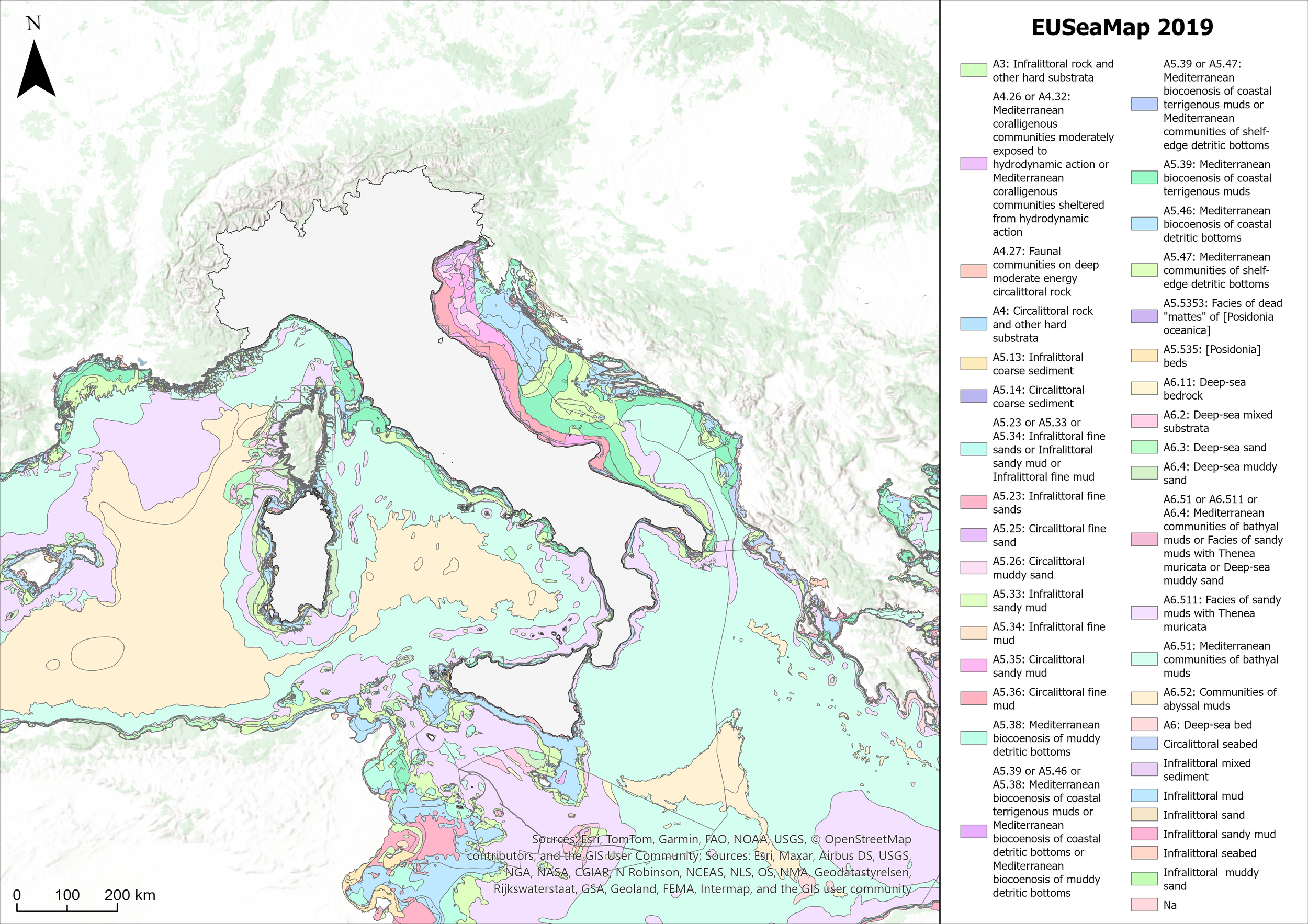
EUSeaMap 2019: modeled distribution of benthic habitats in the Mediterranean Sea based on EUNIS classification.
The analysis focused specifically on areas where the two datasets overlap, thus ensuring a reliable basis for comparison. This approach was necessary because the EUSeaMap model predicts the potential presence of suitable areas for these biocenoses throughout the Italian seas, whereas the HFS data are restricted to selected areas chosen to represent the presence of coralligenous habitat. Moreover, considering the environmental characteristics required by HFS, the following suitable habitats were selected from the EUSeaMap 2019 broad-scale map (Vasquez et al., 2019): A4 (Upper-Circalittoral rock and other hard substrata), A4.26 or A4.32 (Mediterranean coralligenous communities moderately exposed to hydrodynamic action or Mediterranean coralligenous communities sheltered from hydrodynamic action), and A4.27 (Faunal communities on deep moderate energy circalittoral rock) (Davies et al., 2004). These habitats were extracted from the modeled map and, along with the MSFD data, are organized and analyzed in the ArcGIS Pro environment (ESRI Inc.). These input data are shown in Figure 2.
Figure 2
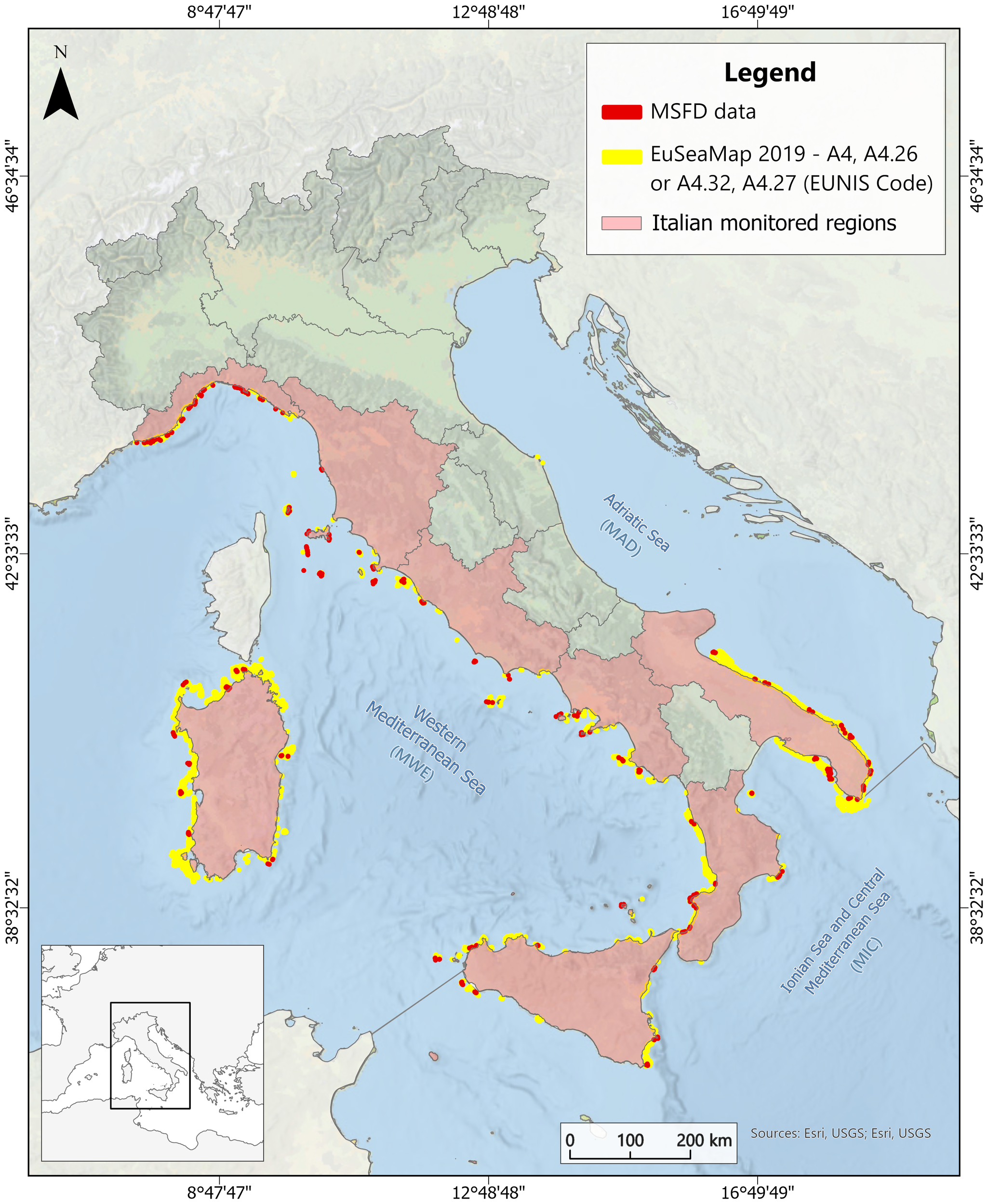
Spatial distributions showing the Italian MSFD coralligenous data (red) and the habitats (A4, A4.26, A4.27, A4.32) extracted from EuSeaMap 2019 (yellow) across the three MSFD marine sub-regions: Western Mediterranean Sea (MWE), Ionian Sea and Central Mediterranean Sea (MIC), and Adriatic Sea (MAD). The map also shows the Italian regions where MSFD coralligenous habitat monitoring was conducted.
2.2 Spatial zonation and data processing
The EUSeaMap broad-scale habitat map and its components, including substratum and bathymetry raster data (Vasquez et al., 2019; Vasquez et al., 2021b), have a resolution of at least 250 meters. Therefore, to address comparison, buffers of different sizes (500, 1000, 1500, and 2000 m) were tested around the areas where the broad-scale map identifies the presence of the habitat. For each buffer, the percentage of MSFD transects falling within the predicted habitat extent (matching) was computed (Figure 3A). To determine the most appropriate threshold, we applied the elbow (knee) method (Thorndike, 1953; Satopaa et al., 2011; Davies et al., 2020; Van Audenhaege et al., 2021; Barve et al., 2023), which combines the evaluation of marginal gains at each additional buffer step (Figure 3B) with the analysis of second-order differences, i.e., the differences between successive marginal gains (Figure 3C). The point where the curve shows a marked decrease in gain and begins to flatten, resembling an elbow, was identified at 1000 m and selected as the optimal threshold (Figure 3C).
Figure 3
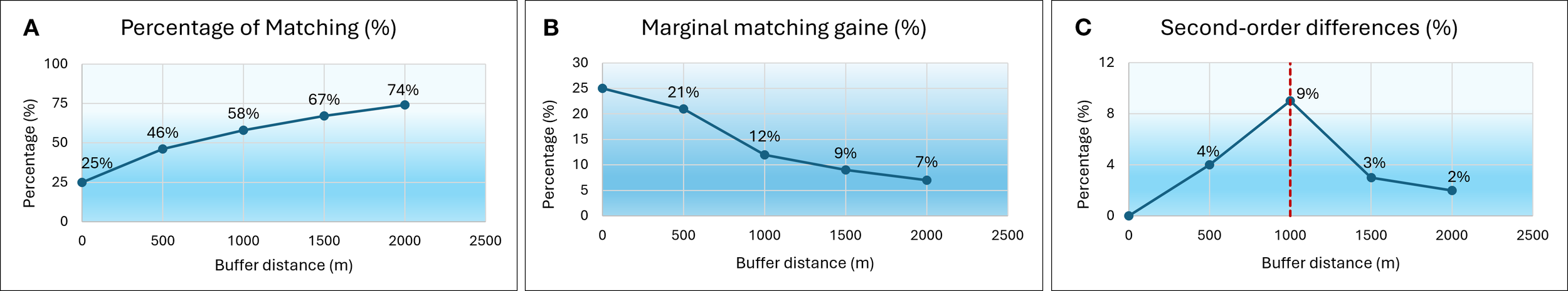
Buffer analysis evaluating the spatial correspondence between MSFD data and the EUSeaMap model. (A) Percentage of matching transects at increasing buffer distances (0–2000 m); (B) Marginal matching gain (%) at each additional buffer step; (C) Second-order differences (%) indicating the elbow point at 1000 m (red dashed line), which is identified as the optimal buffer distance.
Three scenarios were defined: i) areas where EUSeaMap identifies the presence of the selected habitats, which correspond to the core zone; ii) areas within a 1-kilometer buffer around the core zone, which define the buffer zone; and iii) the area between the 1-kilometer buffer and the 12 nautical mile limit, which is designated as the gap zone. Before data comparison, both data sources were converted to the same projection (ETRS 1989 LAEA), following the INSPIRE Directive recommendations for pan-European analyses (European Commission – INSPIRE Maintenance and Implementation Group, 2024). This projected coordinate system allowed for accurate surface and distance estimates, ensuring their suitability for the analysis. The original MSFD datasets, characterized by HFS and derived from the 687 ROV transects, were transformed into polygons by applying 5-meter buffers to ensure that all spatial data had the same spatial geometry for the GIS elaborations. The MSFD data provided not only the presence and distribution of the HFS but also additional information such as bottom type (rocky cliff – RC, biogenic boulders - BB, blocks - B, or both B-BB), slope (horizontal (H), 0°-30° and incline (I), 30°-70°). A total of 86 transects with a rocky cliff (RC) bottom type and a slope with vertical inclination (>70°) were removed from the analysis to avoid bias, as this geomorphological scenario cannot be represented on a 2D map.
2.3 Spatial intersection and scenario assignment
The resulting datasets were spatially intersected to evaluate the percentages of each transect lying within the different analysis zones. An example of an overlay among the three scenarios (core, buffer, and gap zones) and the MSFD transects hosting HFS is shown in Figure 4. Since some transects straddle the core area and/or the buffer zone, the surface of each transect portion lying in both areas was calculated. Where the portion of the transect area within the core zone is greater than 50%, the transect is considered successfully mapped in EUSeaMap (Figure 4B). The same approach is applied to the transects lying between the buffer and the gap zones. In this way, all the MSFD spatial data were matched to the three scenarios.
Figure 4
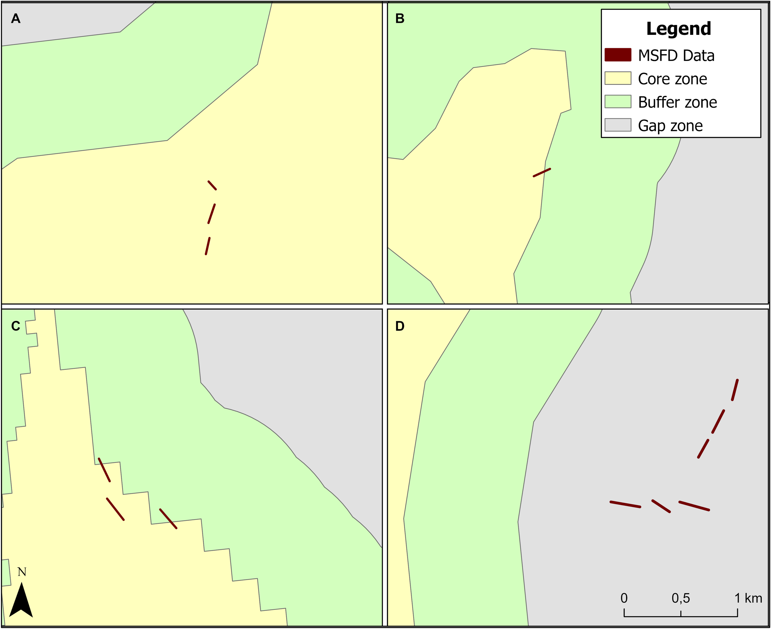
Spatial assignment of MSFD transects across the three analyzed zones: (A) Transects entirely within the core zone; (B) Transect straddling the core and buffer zones, assigned to the core zone; (C) Two transects within the core and buffer zones, and one straddling transect assigned to the buffer zone; (D) Six transects entirely within the gap zone.
The distance between the transects located within the buffer zone and the border of the core zone was calculated considering the nearest point of the geometry, which could be on the vertex, the edge, or the boundary of the polygon. If the geometries overlap, the distance is zero. The resulting spatial relationship was used to determine the percentage of transects that are in close proximity to the core zone.
2.4 Habitat characterization and seabed analysis
As part of the analysis, the frequency of occurrence outside the core zone was calculated through spatial intersection with the EUSeaMap layers, revealing the most represented habitat types (using EUNIS classification present in the modeled map) in the buffer and gap zones. Furthermore, in order to improve the investigation of the cases where the MSFD transects occur in the buffer zone, the most prevalent habitats intersected by the transects were analyzed with respect to the bottom type, seabed slope, and depth values provided by the MSFD data. The latter data (depth values) were also compared with the bathymetric raster information provided by the EMODnet Bathymetry lot. Descriptive statistics, including the mean, median, interquartile range, minimum and maximum values and outliers, were calculated and presented through box plot graphs for bathymetric data. For statistical assessment of the consistency between the two datasets, paired Student’s t-tests were performed to determine whether the mean difference significantly differed from zero. The assumption of normality was tested using the Shapiro-Wilk test. These analyses allowed investigation of the positive or negative influence of bathymetric data on habitat assignment.
3 Results
3.1 Spatial distribution of HFS transects across analysis zones
The MSFD data used in this analysis consist of a total of 601 transects, where the distribution of HFS structuring coralligenous assemblages is known. Among these, 25% of the transects align with the distribution of benthic habitats as predicted by the EUSeaMap model; 32% fall within the buffer zone; and the remaining 43% lie outside both the core and buffer zones, thereby representing data gaps. Notably, 16% of the transects assigned to the buffer zone partially intersect the core zone. If fully accounted for, this would increase compliant distribution by 5%.
As expected, the percentage of transects captured by the model progressively increases with distance from the core zone, reaching its maximum increment at 1 km, where the model captures 58% of the occurrences (Figure 3A).
3.2 EUSeaMap habitat types within the transects in buffer and gap zones
The occurrence of each habitat, as predicted by the model, was assessed within the transects located in both the buffer and gap zones (Figure 5).
Figure 5
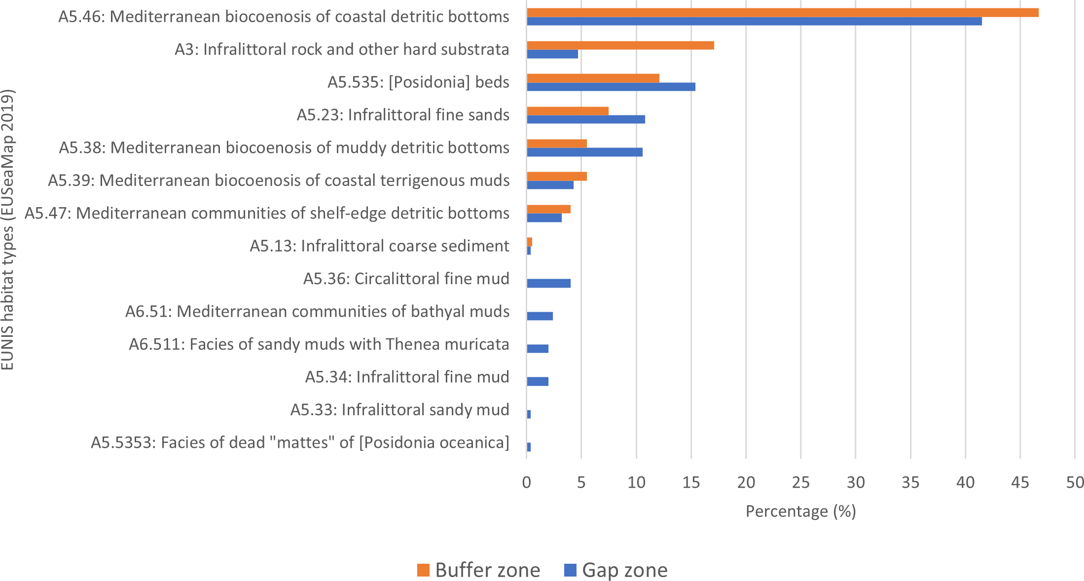
Percentage of EUSeaMap habitats overlapping with MSFD transects in the buffer and gap zones.
In the buffer zone (Figure 5), the three habitats with higher occurrence percentages are as follows: 1) “A5.46 - Mediterranean biocenosis of coastal detritic bottoms” (52%); 2) “A3 - Infralittoral rocks and other hard substrates” (20%) and 3) “A5.535 - Posidonia beds” (14%). Moreover, it is important to note that 55% of these occurrences are attributable to the substrate layer, 15% are due to the biozone, and 30% to both. The gap zone exhibits a similar scenario, where the most represented habitat is A5.46, with the only exception being the A3 percentage, which decreases dramatically. Furthermore, in this case, the most frequent issues are linked to the substratum (60%), with a few cases linked to the biozone (4.5%), and about 35% due to both.
3.3 Seabed characteristics and transects positioning in the buffer zone
For each transect falling in the most represented habitats of the buffer zone scenario, additional information on bottom type, seabed slope and depth presumed by the ground-truth data was considered. The geomorphological MSFD data suggest that these habitats are mostly characterized by the “block and biogenic boulders” bottom type and a horizontal seabed slope (Table 2).
Table 2
| Habitat codes and names (EUNIS 2019) | N° TRANSECTS | BOTTOM TYPE | SLOPE | |||
|---|---|---|---|---|---|---|
| B | BB | B-BB | H | I | ||
| A5.46: Mediterranean biocoenosis of coastal detritic bottoms | 117 | 5% | 13% | 82% | 75% | 25% |
| A3: Infralittoral rock and other hard substrata | 49 | 4% | 25% | 71% | 63% | 37% |
| A5.535: [Posidonia] beds | 28 | 21% | 4% | 75% | 57% | 43% |
Percentage occurrences of different bottom types (B, rocky blocks; BB, biogenic boulders; B–BB, combination of blocks and biogenic boulders) and slope inclinations (H: horizontal slope, 0°; I: inclined slope, 30°–70°) in the three habitats within the buffer zone.
In addition, more than 35% of the transects located entirely in the buffer zone are within 250 meters of the core zone boundary.
3.4 Bathymetric comparison
The comparison between the depth values provided by the ROV and those provided by the EMODnet Bathymetry lot (2019) is reported (Figure 6). This analysis was conducted for all three EUSeaMap habitat types, corresponding to higher transect occurrences in the buffer zone. Box plots highlighted a similar depth range corresponding to A5.46, considering both the interquartile range (IQR) and the outlier values (90th and 10th percentiles). Conversely, the infralittoral habitats A3 and A5.535 do not appear to be comparable when considering the same parameter.
Figure 6
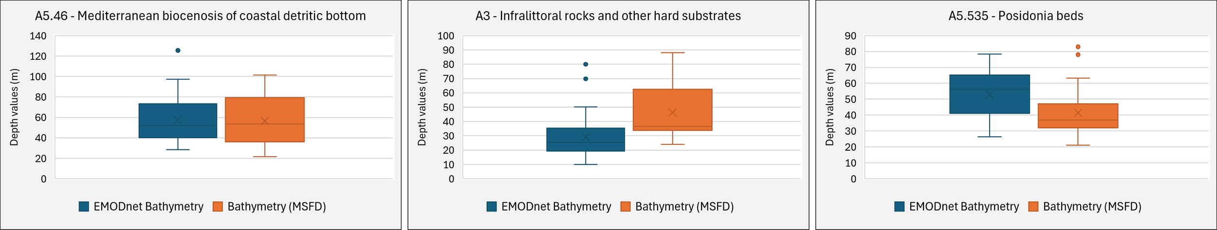
Box plots visually display the distribution of the EMODnet Bathymetry (blue), and the high-resolution (orange) values provided by the MSFD, showing the data quartiles and averages relating to the EUSeaMap 2019 Habitat.
For further assessment of these patterns, paired Student’s t-tests were performed separately for each habitat to test whether the mean differences between EMODnet and ROV depth values significantly differed from zero. The Shapiro-Wilk test indicated that the differences between A3 (n = 36) and A5.46 (n = 92) were not normally distributed (p < 0.05). Nevertheless, given the relatively large sample sizes (n > 30), the paired t-test is considered robust in cases of moderate deviations from normality (Lumley et al., 2002; Kim and Park, 2019). The differences for A5.535 (Posidonia beds, n = 27) did not deviate from normality (Shapiro–Wilk p = 0.21).
The paired t-test results (Table 3) confirmed that the mean difference between EMODnet and MSFD depth values for A5.46 was not significant (p = 0.58). Conversely, the mean differences were significant for A3 (p < 0.001) and A5.535 (p < 0.01), suggesting that the two datasets provided systematically different depth values in these habitats.
Table 3
| Habitat codes and names (EUNIS 2019) | Mean difference | t-value | df | p-value |
|---|---|---|---|---|
| A5.46: Mediterranean biocoenosis of coastal detritic bottoms | 1.0 (-2.7; 4.7) | -0.55 | 91 | 0.58 |
| A3: Infralittoral rock and other hard substrata | -17.3 (-25.0; -9.6) | -4.56 | 35 | <0.001 |
| A5.535: [Posidonia] beds | 11.4 (3.5; 19.3) | 2.96 | 26 | <0.01 |
Results of paired Student’s t-tests comparing EMODnet Bathymetry (2019) and MSFD ground-truth depth measurements for the three most represented habitat types in the buffer zone.
The table reports the mean difference with 95% confidence intervals, t-values, degrees of freedom (df), and associated p-values.
4 Discussion
4.1 Success rate of EUSeaMap vs HFS distribution
This study evaluated the effectiveness of EUSeaMap in defining the distribution of patchy habitats, such as coralligenous, in the Italian seas (Mediterranean Sea). By focusing on the core zone scenario, HFS distribution is successfully detected by the model for 25% of the occurrences. It is interesting to note that, considering the transects partially occur in the core zone (but mainly lie in the buffer zone), this percentage increases up to 30%. Additionally, by considering the transects entirely hosted by the buffer zone but located within 250 meters from the core zone, this percentage rises to 40%.
4.2 Interpreting habitat occurrences in the buffer zone
The main modeled habitats occurring along the transects must be evaluated considering the specificity of the coralligenous patterns and morphology, including their complexity and three-dimensional bioconstructions (Figure 7A), and that these assemblages can exist not only as a sole habitat on the seafloor, but also as part of mosaic patterns with other habitats, such as coastal detritic bottom and Posidonia oceanica meadows (Bracchi et al., 2017; Di Iorio et al., 2021; Varzi et al., 2023; Astruch et al., 2025). A5.46 is the predominant habitat in both the buffer and gap zones, in agreement with recent studies (Bracchi et al., 2017; Chimienti et al., 2021; Piazzi et al., 2022; Enrichetti et al., 2023a), which describe how coastal detritic bottoms often surround coralligenous outcrops, serving as reliable proxies for their presence and supporting associations with other habitat types. Therefore, HFS can thrive near and on detritic substrates, often extending across biogenic constructions (Cerrano et al., 2001; Valisano et al., 2019; Enrichetti et al., 2023b). Furthermore, as highlighted by Varzi et al. (2023), extensive areas where coralligenous outcrops and detritic bottoms coexist have been classified as coralligenous patches of detritic bottom habitats. Similarly, Astruch et al. (2023) reported that several octocorals, including Eunicella singularis (Esper, 1791), Eunicella verrucosa (Pallas, 1766), Leptogorgia sarmentosa (Esper, 1791), and large calcified bryozoan species such as Pentapora fascialis (Pallas, 1766), are frequently observed developing on coarse detritic bottom habitats, contributing to the formation of complex and interconnected ecological systems in the Mediterranean Sea (Figure 7B). These findings are in line with the results presented in Table 2, where 83% of the analyzed transects are characterized by a block and biogenic boulders bottom type. The analysis of transects in the buffer zone also revealed that, following the A5.46 habitat, the A3 - Infralittoral rocks and other hard substrates, and “A5.535 - Posidonia beds” habitats also showed significant occurrences. Regarding the A3 habitat, the choice of substrate (rocks and hard substratum) is coherent; however, the biozone boundary is inaccurate, even if some of the HFS, under specific environmental conditions, may be present in the lower infralittoral zone, characterizing a habitat that is well-known for its intermediate characteristics, between the Infralittoral and Circalittoral zones, called “pre-coralligenous” (Figure 7C) (Ballesteros, 2003; Cinelli and Tunesi, 2009; Varzi et al., 2023). For the A5.535 habitat, the biozone assignment is similarly characterized by incoherence. Nevertheless, the Posidonia layers in EUSeaMap represent input data and are derived from the integration of available survey maps, which vary significantly in resolution and age. However, Posidonia meadows, with their “mattes”, may coexist with coralligenous assemblages, since these habitats are frequently intermixed within a spatially heterogeneous rocky environment (Figure 7D) (Albano and Sabelli, 2011; Valisano et al., 2019).
Figure 7
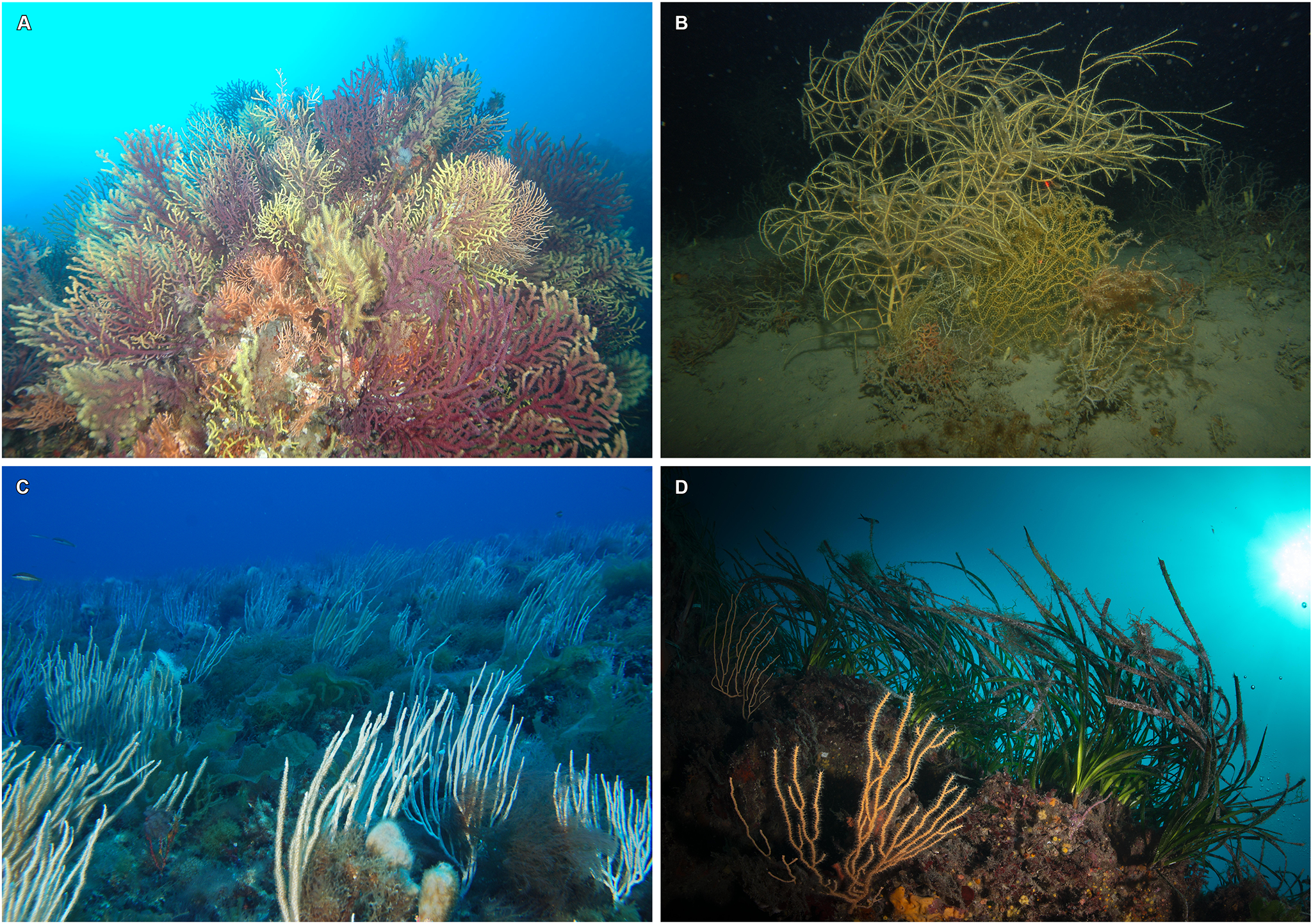
Images illustrating the distribution of HFS in different habitat types: (A) Typical coralligenous assemblage with complex three-dimensional structure; (B)Leptogorgia sarmentosa growing on coarse detritic bottoms; (C)Eunicella singularis occurring in lower infralittoral environments (“pre-coralligenous”); (D) Association of HFS (Eunicella cavolini) with Posidonia oceanica habitats (image reproduced with permission).
4.3 The role of bathymetry in habitat classification
Considering that the infra/circalittoral biozone boundary is estimated based on the light availability at the sea bottom, which is also evaluated using depth, it is easy to understand why the boundary strongly depends on the bathymetry values provided in the model (EMODnet Bathymetry Consortium, 2019; Vasquez et al., 2015). The results of the bathymetric comparison between the two datasets suggest that the A3 and A5.535 habitats show a less consistent relationship, reflecting the morphology that typically defines these habitats. The A3 habitat is often found in areas with high morphological variability and steep slopes, characterized by irregular and rugged substrates, which makes it challenging to produce reliable bathymetric representations using broad-scale data (100-meter resolution). Similarly, the bathymetric variability of the lower limit of the Posidonia oceanica meadow reflects its inherently variable nature, with a wide range of substratum typologies, and is closely linked to in situ transparency of the water (Montefalcone et al., 2014). In particular, the 100-meter resolution EMODnet Bathymetry grid, derived through pre-gridding of survey data, gap-filling interpolation, and harmonization of multiple data sources, is too coarse to portray heterogeneous morphology and, consequently, fine-scale seabed features (EMODnet Bathymetry Consortium, 2024). As a result, in complex coastal environments, depth gradients and ecological thresholds can appear shifted (i.e., Posidonia distribution deeper than expected from ecological knowledge, as illustrated in Figure 6).
Conversely, the bathymetric datasets for the A5.46 habitat appear highly consistent. This is in line with the characteristics of the substrate of this habitat, which is defined by flat and regular morphological features (Bo et al., 2009).
4.4 Implications and perspectives
The findings of this study demonstrate that a broad-scale map, such as EUSeaMap, is moderately effective in representing and identifying discontinuous habitats. Nonetheless, considering the challenges associated with environmental input variables and map scale, the outcome can be regarded as satisfactory, thereby confirming the value of this product for investigating and delineating the potential distribution of complex habitats, such as coralligenous reefs. The results also suggest which input data need to be improved in order to enhance the model’s performance. In particular, future improvements should prioritize the integration of a more detailed substrate layer from the EMODnet Geology, since the geological nature of the seabed is a critical determinant in identifying the distribution of benthic habitats (Roff et al., 2003; Valentine, 2019; Franz et al., 2021; Fraschetti et al., 2024). These, in turn, represent a fundamental environmental condition, alongside bathymetry and water transparency, for predicting the presence of habitat-forming species such as those that are characteristic of coralligenous reefs or offshore rocky outcrops (e.g., black coral assemblages) (Fiorentino et al., 2021; Lillis et al., 2021). Future technological advancements are expected to improve significantly the quality of model input data, particularly in terms of the diffuse attenuation coefficient (Kdpar) and bathymetry resolution, thereby addressing many of the current limitations and enabling more effective mapping of seabed habitats. This study represents a pioneering effort to compare and test systematically a modeled map against high-resolution data and establishes a benchmark for future applications.
Moreover, the use of EUSeaMap by various stakeholders across multiple applications (e.g., implementation of EU directives, European-scale assessments) is not only due to the product’s uniqueness but also to its overall quality as regards the identification of patchy habitats such as coralligenous assemblages and, to a greater degree, the representation of habitats with a wider and more homogeneous distribution, where its predictive capacity can be more effectively expressed.
Ultimately, the study enhances confidence in EUSeaMap, suggesting that its application can be extended and promoted in new fields, and also supports broader application to future marine management and conservation initiatives.
Statements
Data availability statement
Publicly available datasets were analyzed in this study. This data can be found here: https://emodnet.ec.europa.eu/geonetwork/srv/api/records/01bf1f24-fdcd-4ee7-af8b-e62cf72fe2f9http://www.db-strategiamarina.isprambiente.it/app/#/.
Author contributions
MR: Data curation, Software, Conceptualization, Methodology, Writing – original draft, Formal analysis. AA: Formal analysis, Software, Methodology, Resources, Writing – review & editing, Validation, Data curation. SA: Methodology, Supervision, Formal analysis, Writing – review & editing, Resources, Software, Data curation, Conceptualization, Project administration, Funding acquisition, Validation. MG: Resources, Validation, Writing – review & editing. MA: Resources, Validation, Writing – review & editing. LT: Funding acquisition, Resources, Writing – review & editing, Project administration, Validation, Supervision.
Funding
The author(s) declare financial support was received for the research and/or publication of this article. The author(s) declare that Directorate-General for Maritime Affairs and Fisheries of the European Commission (DG MARE) funded the EMODnet Seabed Habitats initiative, while ground truth data collection were funded by the Italian Ministry for the Environment under the National Marine Strategy Framework Directive monitoring program.
Acknowledgments
The authors would like to thank the Regional Agencies for Environmental Protection (Agenzie Regionali per la Protezione dell’Ambiente), for the field work. Special thanks are due to Daniele Corsini for granting permission to use the image “D” shown in Figure 7. The original image is available at: https://marevivo.it/tutela-della-biodiversita-approfondimenti/posidonia/.
Conflict of interest
The author(s) declare that the research was conducted in the absence of any commercial or financial relationships that could be construed as a potential conflict of interest.
Generative AI statement
The author(s) declare that no Generative AI was used in the creation of this manuscript.
Any alternative text (alt text) provided alongside figures in this article has been generated by Frontiers with the support of artificial intelligence and reasonable efforts have been made to ensure accuracy, including review by the authors wherever possible. If you identify any issues, please contact us.
Publisher’s note
All claims expressed in this article are solely those of the authors and do not necessarily represent those of their affiliated organizations, or those of the publisher, the editors and the reviewers. Any product that may be evaluated in this article, or claim that may be made by its manufacturer, is not guaranteed or endorsed by the publisher.
References
1
Albano P. G. Sabelli B. (2011). Comparison between death and living mollusks assemblages in a Mediterranean infralittoral off-shore reef. Palaeogeogr. Palaeoclimatol. Palaeoecol.310, 206–215. doi: 10.1016/j.palaeo.2011.07.012
2
Andersen J. H. Manca E. Agnesi S. Al-Hamdani Z. Lillis H. Mo G. et al . (2018). European broad-scale seabed habitat maps support implementation of ecosystem-based management. Open J. Ecol.8, 86–103. doi: 10.4236/oje.2018.82007
3
Angiolillo M. Fortibuoni T. (2020). Impacts of marine litter on Mediterranean reef systems: from shallow to deep waters. Front. Mar. Sci7. doi: 10.3389/fmars.2020.581966
4
Astruch P. Boudouresque C. F. Cabral M. Schohn T. Ballesteros E. Bellan-Santini et al . (2025). An ecosystem-based index for Mediterranean coralligenous reefs: A protocol to assess the quality of a complex key habitat. Mar. pollut. Bull.220, 118375. doi: 10.1016/j.marpolbul.2025.118375
5
Astruch P. Orts A. Schohn T. Belloni B. Ballesteros E. Bănaru D. et al . (2023). Ecosystem-based assessment of a widespread Mediterranean marine habitat: The Coastal Detrital Bottoms, with a special focus on epibenthic assemblages. Front. Mar. Sci10, 1130540. doi: 10.3389/fmars.2023.1130540
6
Ballesteros E. (2003). - The coralligenous in the Mediterranean Sea (Tunis, Tunisia: RAC/SPA- Regional Activity Centre for Specially Protected Areas).
7
Ballesteros E. (2006). Mediterranean coralligenous assemblages: a synthesis of present knowledge,” in Oceanography and Marine Biology: an annual review, vol. 44, 123–195. Boca Raton, FL, USA: Taylor & Francis.
8
Barve S. Webster J. M. Chandra R. (2023). Reef-insight: a framework for reef habitat mapping with clustering methods using remote sensing. Information14, 373. doi: 10.3390/info14070373
9
Bo M. Bavestrello G. Canese S. Giusti M. Salvati E. Angiolillo M. et al . (2009). Characteristics of a black coral meadow in the twilight zone of the central Mediterranean Sea. Mar. Ecol. Prog. Ser.397, 53–61. doi: 10.3354/meps08185
10
Bracchi V. A. Basso D. Marchese F. Corselli C. Savini A. (2017). Coralligenous morphotypes on subhorizontal substrate: A new categorization. Continent. Shelf. Res.144, 10–20. doi: 10.1016/j.csr.2017.06.005
11
Bramanti L. Benedetti M. C. Cupido R. Cocito S. Priori C. Erra F. et al . (2017). “ Demography of animal forests: the example of mediterranean gorgonians,” in Marine Animal Forests: The Ecology of Benthic Biodiversity Hotspots. Eds. RossiS.BramantiL.GoriA.Orejas Saco del ValleC. (Cham, Switzerland: Springer), 1–20. doi: 10.1007/978-3-319-17001-5_13-1
12
Callery O. Grehan A. (2023). Extending regional habitat classification systems to ocean basin scale using predicted species distributions as proxies. Front. Mar. Sci10. doi: 10.3389/fmars.2023.1139425
13
Cerrano C. Bavestrello G. Bianchi C. N. Calcinai B. Cattaneo-Vietti R. Morri C. et al . (2001). “ The role of sponge bioerosion in Mediterranean coralligenous accretion,” in Mediterranean Ecosystems: Structures and Processes ( Springer Milan, Milano), 235–240.
14
Chimienti G. Aguilar R. Maiorca M. Mastrototaro F. (2021). A newly discovered forest of the whip coral Viminella flagellum (Anthozoa, Alcyonacea) in the Mediterranean Sea: a non-invasive method to assess its population structure. Biology11, p.39. doi: 10.3390/biology11010039
15
Cinelli F. Tunesi L. (2009). The coralligenous domain. In Marine Bioconstructions – Nature’s Architectural Seascapes. Ed. ReliniG., (Udine, Italy: Ministero dell’Ambiente e della Tutela del Territorio e del Mare – Museo Friulano di Storia Naturale). 13–27.
16
Davies C. E. Moss D. Hill M. O. (2004). EUNIS habitat classification revised 2004. Report to: European environment agency-European topic center on nature protection and biodiversity, 127–143. Copenhagen, Denmark: European Environment Agency (EEA).
17
Davies H. N. Gould J. Hovey R. K. Radford B. Kendrick G. A. Anindilyakwa Land et al . (2020). Mapping the marine environment through a cross-cultural collaboration. Front. Mar. Sci7, 716. doi: 10.3389/fmars.2020.00716
18
de la Torriente A. González-Irusta J. M. Aguilar R. Fernández-Salas L. M. Punzón A. Serrano A. (2019). Benthic habitat modelling and mapping as a conservation tool for marine protected areas: A seamount in the western Mediterranean. Aquat. Conserv.: Mar. Freshw. Ecosyst.29, pp.732–pp.750. doi: 10.1002/aqc.3075
19
Di Iorio L. Audax M. Deter J. Holon F. Lossent J. Gervaise C. et al . (2021). Biogeography of acoustic biodiversity of NW Mediterranean coralligenous reefs. Sci. Rep.11, 16991. doi: 10.1038/s41598-021-96378-5
20
Di Stefano F. Molinari A. Radicioli M. Strollo A. Proietti R. Giusti M. et al (2024). Main results of coralligenous monitoring within the implementation of Marine Strategy Framework Directive in Italy. In: PontiM.CerranoC.WörheideG. (Eds.), Naples, Italy, Città della Scienza & Stazione Zoologica Anton Dohrn2–5, 292. doi: 10.5281/zenodo.13823192
21
EMODnet Bathymetry Consortium (2019). - High Resolution Seabed Mapping - WP2: Generate indicators in the DTM - Use of the dataset Quality Index to expand services associated to the EMODnet DTM. French Research Institute for Exploitation of the Sea (Ifremer), Brest, France.
22
EMODnet Bathymetry Consortium (2024). EMODnet Digital Bathymetry (DTM 2024). Flanders Marine Institute (VLIZ), Ostend, Belgium. doi: 10.12770/cf51df64-56f9-4a99-b1aa-36b8d7b743a1
23
Enrichetti F. Bavestrello G. Cappanera V. Mariotti M. Massa F. Merotto L. et al . (2023a). High megabenthic complexity and vulnerability of a mesophotic rocky shoal support its inclusion in a Mediterranean MPA. Diversity15, 933. doi: 10.3390/d15080933
24
Enrichetti F. Toma M. Bavestrello G. Betti F. Giusti M. Canese S. et al . (2023b). Facies created by the yellow coral Dendrophyllia cornigera (Lamarck 1816): Origin, substrate preferences and habitat complexity. Deep. Sea. Res. Part I.: Oceanogr. Res. Papers.195, 104000. doi: 10.1016/j.dsr.2023.104000
25
European Commission (2008). - Directive 2008/56/EC of the European Parliament and of the Council of 17 June 2008. Establishing a framework for community action in the field of marine environmental policy (Marine Strategy Framework Directive). Off. J. Europ. Union. L164, 19–40.
26
European Commission – INSPIRE Maintenance and Implementation Group (2024). INSPIRE Data Specification on Coordinate Reference Systems – Technical Guidelines (D2.8.I.1, version 3.4.0) (Luxembourg: Publications Office of the European Union), L164, 19–40. Publications Office of the European Union, Luxembourg City, Luxembourg. Available online at: https://inspire-mif.github.io/technical-guidelines/data/rs/dataspecification_rs.pdf (Accessed September 20, 2025).
27
Fiorentino A. Battaglini L. D’Angelo S. (2021). EMODnet collation of geological events data provides evidence of their mutual relationships and connections with underlying geology: a few examples from Italian seas. Q. J. Eng. Geol. Hydrogeolo.54, qjegh2019–147. doi: 10.1144/qjegh2019-147
28
Foster N. L. Rees S. Langmead O. Griffiths C. Oates J. Attrill M. J. (2017). Assessing the ecological coherence of a marine protected area network in the Celtic Seas. Ecosphere8, e01688. doi: 10.1002/ecs2.1688
29
Franz M. von Rönn G. A. Barboza F. R. Karez R. Reimers H. C. Schwarzer K. et al . (2021). How do geological structure and biological diversity relate? Benthic communities in boulder fields of the Southwestern Baltic Sea. Estuaries. Coasts.44, 1994–2009. doi: 10.1007/s12237-020-00877-z
30
Fraschetti S. Strong J. Buhl-Mortensen L. Foglini F. Goncalves J. Goncalez-Irusta J. M. et al . (2024). “ Marine habitat mapping. EMB Future Science Brief, 11,” in European Marine Board (Ostend, Belgium: European Marine Board), 76. doi: 10.5281/zenodo.11203128
31
Gili J. M. Murillo J. Ros J. (1989). The distribution pattern of benthic Cnidarians in the Western Mediterranean. Sci. Mar.53, 19–35.
32
Gimenez G. Corriero G. Beqiraj S. Lazaj L. Lazic T. Longo C. et al . (2022). Characterization of the coralligenous formations from the Marine Protected Area of Karaburun-Sazan, Albania. J. Mar. Sci Eng.10, 1458. doi: 10.3390/jmse10101458
33
Gori A. Bavestrello G. Grinyó J. Dominguez-Carrió C. Ambroso S. Bo M. (2017). Animal forests in deep coastal bottoms and continental shelf of the Mediterranean Sea. Mar. Anim. Forests.: Ecol. Benthic. Biodivers. Hotspots., 1–27. Cham: Springer. doi: 10.1007/978-3-319-17001-5_5-1
34
Gottlieb B. Pruckner S. Anthony B. P. (2024). An ecological coherence assessment of the Wider Caribbean Region marine protected area network. Ocean. Coast. Manage.255, 107249. doi: 10.1016/j.ocecoaman.2024.107249
35
Ingrosso G. Abbiati M. Badalamenti F. Bavestrello G. Belmonte G. Cannas R. et al . (2018). Mediterranean bioconstructions along the Italian coast. Adv. Mar. Biol.79, 61–136. doi: 10.1016/bs.amb.2018.05.001
36
Kim T. K. Park J. H. (2019). More about the basic assumptions of t-test: normality and sample size. Korean. J. Anesthesiol.72, 331–335. doi: 10.4097/kja.d.18.00292
37
Laubier L. (1966). Le coralligène des Albères. Monographie biocénotique. Annales de l’Institut Océanographique43, 137–316. Institut Océanographique, Paris, France.
38
Lillis H. Allen H. Agnesi S. Annunziatellis A. Vasquez M. (2021). A combined, harmonized data product showing the best evidence for the extent of biogenic substrate in Europe. Ref. D3.06 - EASME/EMFF/2018/1.3.1.8/Lot2/SI2.810241 – EMODnet Seabed Habitats. Available online at: https://archimer.ifremer.fr/doc/00736/84820/ (Accessed September 20, 2025).
39
Lombardi C. Taylor P. D. Cocito S. (2020). “ Bryozoans: the ‘forgotten’ bioconstructors,” in Perspectives on the marine animal forests of the world, 193–217. Springer, Cham, Switzerland. doi: 10.1007/978-3-030-57054-5_7
40
Lumley T. Diehr P. Emerson S. Chen L. (2002). The importance of the normality assumption in large public health data sets. Annu. Rev. Public Health23, 151–169. doi: 10.1146/annurev.publhealth.23.100901.140546
41
MATTM-ISPRA (2019). - Schede Metodologiche per l’attuazione delle Convenzioni stipulate tra Ministero dell’Ambiente e della Tutela del Territorio e del Mare e Agenzie Regionali per la protezione dell’Ambiente. Modulo 7 Habitat Coralligeno. Programmi di Monitoraggio per la Strategia Marina, Art. 11, D. lgs. 190/2010. ISPRA – Istituto Superiore per la Protezione e la Ricerca Ambientale, Rome, Italy.
42
Montefalcone M. Tunesi L. Ouerghi E. (2021). A review of the classification systems for marine benthic habitats and the new updated Barcelona Convention classification for the Mediterranean. Mar. Environ. Res.Elsevier, Amsterdam, Netherlands, 169–105387. doi: 10.1016/j.marenvres.2021.105387. 16.
43
Montefalcone M. Vacchi M. Schiaffino C. F. Morri C. Cristina C. Cabella R. et al . (2014). “ May. Meadow development of the seagrass Posidonia oceanica on the rocky seabed: a preliminary study in the Ligurian Sea,” In EGU General Assembly Conference Abstracts (Vol. 16, p. 8714). Göttingen, Germany: Copernicus GmbH (on behalf of the European Geosciences Union).
44
Pérès J. M. Picard J. (1964). Nouveau manuel de bionomie benthique de la mer Méditerranée (Marseille, France: Station Marine d’Endoume) 31 (47), 1–137.
45
Piazzi L. Ferrigno F. Guala I. Cinti M. F. Conforti A. De Falco G. et al . (2022). Inconsistency in community structure and ecological quality between platform and cliff coralligenous assemblages. Ecol. Indic.136, 108657. doi: 10.1016/j.ecolind.2022.108657
46
Pierdomenico M. Bonifazi A. Argenti L. Ingrassia M. Casalbore D. Aguzzi L. et al . (2021). Geomorphological characterization, spatial distribution and environmental status assessment of coralligenous reefs along the Latium continental shelf. Ecol. Indic.131, 108219. doi: 10.1016/j.ecolind.2021.108219
47
Populus J. Vasquez M. Albrecht J. Manca E. Agnesi S. Al Hamdani Z. et al . (2017). EUSeaMap. A European broad-scale seabed habitat map. French Research Institute for Exploitation of the Sea (Ifremer), Brest, France. doi: 10.13155/49975
48
Radicioli M. Angiolillo M. Giusti M. Proietti R. Fortibuoni T. Silvestri C. et al . (2022). “Monitoring coralligenous reefs in Italian coastal waters within the Marine Strategy Framework Directive,” in Proceedings of the 4th Mediterranean Symposium on the Conservation of Coralligenous & Other Calcareous Bio-Concretions (Genoa, Italy, 20–21 September 2022). UNEP/MAP – SPA/RAC, Tunis, Tunisia. 96.
49
Roff J. C. Taylor M. E. Laughren J. (2003). Geophysical approaches to the classification, delineation and monitoring of marine habitats and their communities. Aquat. Conserv.: Mar. Freshw. Ecosyst.13, 77–90. doi: 10.1002/aqc.525
50
Rossi S. Bramanti L. Gori A. Orejas C. (2017). An overview of the animal forests of the world. Mar. Anim. Forests., 1–26. doi: 10.1007/978-3-319-17001-5_1-1
51
Rosso A. DI E. M. (2023). Capturing the moment: a snapshot of Mediterranean bryozoan diversity in the early, (2023). Mediterr. Mar. Sci24, pp.426–pp.445. doi: 10.12681/mms.34329
52
Satopaa V. Albrecht J. Irwin D. Raghavan B. (2011). Finding a” kneedle” in a haystack: Detecting knee points in system behavior. Proceedings of the 31st International Conference on Distributed Computing Systems Workshops (ICDCSW). IEEE, Los Alamitos, CA, USA. doi: 10.1109/ICDCSW.2011.20
53
SNPA (2024). Schede metodologiche utilizzate nei programmi di monitoraggio del secondo ciclo della Direttiva Strategia Marina (D.M. 2 febbraio 2021) (Rome, Italy: Pubblicazione tecnica SNPA), ISBN: 978-88-448-1236-2.
54
Thorndike R. L. (1953). Who belongs in the family? Psychometrika18, 267–276. doi: 10.1007/BF02289263
55
Tunesi L. Agnesi S. Cameron A. Coltman N. Hamdi A. Lopez V. et al . (2010). EUSeaMap project: modelling European seabed habitats-a focus on the western Mediterranean. Rapp. Commun. Int. Mer. Médit.39, 686.
56
Valentine P. C. (2019). Sediment classification and the characterization, identification, and mapping of geologic substrates for the glaciated Gulf of Maine seabed and other terrains, providing a physical framework for ecological research and seabed management (No. 2019-5073) (Reston, VA: US Geological Survey). doi: 10.3133/sir20195073
57
Valisano L. Palma M. Pantaleo U. Calcinai B. Cerrano C. (2019). Characterization of North–Western Mediterranean coralligenous assemblages by video surveys and evaluation of their structural complexity. Mar. pollut. Bull.148, 134–148. doi: 10.1016/j.marpolbul.2019.07.012
58
Van Audenhaege L. Broad E. Hendry K. R. Huvenne V. A. (2021). High-resolution vertical habitat mapping of a deep-sea cliff offshore Greenland. Front. Mar. Sci8, 669372. doi: 10.3389/fmars.2021.669372
59
Varzi A. G. Fallati L. Savini A. Bracchi V. A. Bazzicalupo P. Rosso A. et al . (2023). Geomorphology of coralligenous reefs offshore southeastern Sicily (Ionian Sea). J. Maps.19, 2161963. doi: 10.1080/17445647.2022.2161963
60
Vasquez M. Agnesi S. Al Hamdani Z. Annunziatellis A. Askew N. Bekkby T. et al . (2021b). Mapping seabed habitats over large areas: prospects and limits. EMODnet Thematic Lot n° 2 – Seabed Habitats. D1.15. EASME/EMFF/2018/1.3.1.8/Lot2/SI2.810241. doi: 10.13155/78021
61
Vasquez M. Allen H. Manca E. Castle L. Lillis H. Agnesi S. et al . (2021a). EUSeaMap 2021. A European broad-scale seabed habitat map. D1.13 EASME/EMFF/2018/1.3.1.8/Lot2/SI2.810241– EMODnet Thematic Lot n° 2 – Seabed Habitats EUSeaMap 2021 - Technical Report. French Research Institute for Exploitation of the Sea (Ifremer), Brest, France French Research Institute for Exploitation of the Sea (Ifremer), Brest, France. doi: 10.13155/83528
62
Vasquez M. Manca E. Inghilesi R. Martin S. Agnesi S. Al Hamdani Z. et al . (2019). EUSeaMap 2019. A European broad-scale seabed habitat map, Technical Report. French Research Institute for Exploitation of the Sea (Ifremer), Brest, France.
63
Vasquez M. Mata Chacon D. Tempera F. O’keeffe E. Galparsoro I. Sanz Alonso J. et al . (2015). Broad-scale mapping of seafloor habitats in the north-east Atlantic using existing environmental data. J. Sea. Res.100, 120–132. doi: 10.1016/j.seares.2014.09.011
64
Villa F. Tunesi L. Agardy T. (2002). Optimal zoning of marine protected areas through spatial multiple criteria analysis: the case of the Asinara Island National Marine Reserve of Italy. Conserv. Biol.16, 1–12. doi: 10.1046/j.1523-1739.2002.00425.x
65
Zapata F. Goetz F. E. Smith S. A. Howison M. Siebert S. Church S. H. et al . (2015). Phylogenomic analyses support traditional relationships within Cnidaria. PloS One10, e0139068. doi: 10.1371/journal.pone.0139068
66
Zapata-Ramirez P. A. Huete-Stau_Er C. Scaradozzi D. Marconi M. Cerrano C. (2016). - Testing methods to support management decisions in coralligenous and cave environments. A case study at Portofino MPA. Mar. Environ. Res.118, 45–56. doi: 10.1016/j.marenvres.2016.04.010
Summary
Keywords
EMODnet Seabed Habitats, modeled map, coralligenous, Marine Strategy Framework Directive, high-resolution data, Mediterranean Sea
Citation
Radicioli M, Annunziatellis A, Agnesi S, Giusti M, Angiolillo M and Tunesi L (2025) Evaluating broad-scale habitat model against patchy benthic habitats: the case of EUSeaMap. Front. Mar. Sci. 12:1648922. doi: 10.3389/fmars.2025.1648922
Received
17 June 2025
Accepted
23 September 2025
Published
22 October 2025
Volume
12 - 2025
Edited by
Stanislao Bevilacqua, University of Trieste, Italy
Reviewed by
Patrick Astruch, GIS Posidonie, France; Silvija Kipson, SEAFAN - Marine Research & Consultancy, Croatia
Updates
Copyright
© 2025 Radicioli, Annunziatellis, Agnesi, Giusti, Angiolillo and Tunesi.
This is an open-access article distributed under the terms of the Creative Commons Attribution License (CC BY). The use, distribution or reproduction in other forums is permitted, provided the original author(s) and the copyright owner(s) are credited and that the original publication in this journal is cited, in accordance with accepted academic practice. No use, distribution or reproduction is permitted which does not comply with these terms.
*Correspondence: Martina Radicioli, martina.radicioli@isprambiente.it
Disclaimer
All claims expressed in this article are solely those of the authors and do not necessarily represent those of their affiliated organizations, or those of the publisher, the editors and the reviewers. Any product that may be evaluated in this article or claim that may be made by its manufacturer is not guaranteed or endorsed by the publisher.