Abstract
The Southern Temperate Zone (STZ, 30°S–55°S) plays a crucial role in global energy, water, and carbon cycles. While the Earth System Models (ESMs) of phase 6 of the Coupled Model Intercomparison Project (CMIP6) provide essential data for climate research focused on the Southern Hemisphere, significant inter-model discrepancies still necessitate a comprehensive evaluation, especially in the STZ. This study employs a multivariable integrated evaluation (MVIE) method to assess 17 CMIP6 ESMs in simulating the near-surface atmospheric fields and the oceanic temperature and salinity fields over the STZ, enabling holistic assessment of multiple variables. The multi-model ensemble (MME) mean of the near-surface atmospheric fields exhibits systematic biases, including overestimated westerly winds, northerly winds, and specific humidity. For the oceanic fields, pervasive warm biases in the potential temperature have been found in the deep ocean, whereas fresh biases in the salinity have been identified in the deep layer. According to the results of the MVIE, ten models show relatively good performance in simulating climatological annual means. Based on integrated statistical indices, eight models (ACCESS-ESM1-5, CanESM5, CanESM5-CanOE, CNRM-ESM2-1, GFDL-ESM4, MRI-ESM2-0, NorESM2-LM, NorESM2-MM) rank ahead among 17 CMIP6 ESMs. Evaluation of the seasonal climatology indicates that ESMs generally exhibit better performance during the austral summer than in winter. GFDL-ESM4 performs best in summer and autumn, whereas MPI-ESM1-2-HR and NorESM2-MM excel in winter, and MPI-ESM1-2-HR leads in spring. The study reveals persistent challenges in CMIP6 ESMs for simulating deep-ocean processes in the STZ.
1 Introduction
The mid-latitude region in the Southern Hemisphere, generally recognized as the Southern Temperate Zone (STZ), plays a crucial role in the global climate system (Simmonds and King, 2004; Cai et al., 2023; Fogt and Marshall, 2020). The oceans in the STZ contribute substantially to the global carbon cycle, acting as major carbon sinks that absorb excess atmospheric heat and anthropogenic carbon emissions (Khatiwala et al., 2009; Tjiputra et al., 2010; Yang et al., 2019). The northern flank of the Antarctic Circumpolar Current (ACC), recognized as the strongest current in the world’s oceans (Barker and Thomas, 2004), flows through the STZ and is associated with steeply tilted isopycnal surfaces in the meridional direction (Böning et al., 2008). Westerlies in the STZ are also the strongest time-mean oceanic winds globally (Russell et al., 2006). The intensification and poleward shift of westerlies are accompanied by a poleward and upward shift and intensification of the storm tracks. This results in more low clouds, poleward shifts in precipitation, and enhanced poleward eddy energy flux at high latitudes (Korhonen et al., 2010; Hendon et al., 2007; Thompson et al., 2011; Yin, 2005; Goyal et al., 2021; Chemke et al., 2022). Due to the complex air-sea interactions, large-scale sea surface temperature (SST) anomalies in the STZ are influenced by modes of atmospheric variability (Kushnir et al., 2002), and midlatitude SST anomalies may also affect the storm track and strength (Kushnir et al., 2002; Czaja et al., 2019). In addition, in the STZ, the ACC and westerlies also influence the marine biota and ecosystems in the Southern Ocean and beyond by regulating the distribution of nutrients and dispersals of diverse species (Sanmartín et al., 2007; Hunt et al., 2016). Due to the sparsity of observations in the Southern Ocean, ESMs provide insights into the investigations of long-term changes and predictions of the complex climate system in the Southern Ocean.
The Coupled Model Intercomparison Project (CMIP) was established for the investigation and comparisons between coupled ocean-atmosphere-cryosphere-land general circulation models (Meehl et al., 2000). The CMIP6 comprises over 100 ESMs and a series of experiments (Eyring et al., 2016), including CMIP historical simulations (1850-2014) and future scenario experiments. Compared to previous CMIP Phases, contemporary models in CMIP6 present improved estimation in simulating the surface wind stress in the Southern Hemisphere, with stronger and less equatorward-biased winds (Beadling et al., 2020). Meanwhile, the ACC transport in the CMIP6 models largely falls within observational uncertainty in the Southern Ocean (Beadling et al., 2020). By comparing historical experiments with future global warming scenarios, Fahad et al. (2020) suggested that projected intensification of southern-hemisphere subtropical anticyclones would intensify in strength at their southern flank and center. Purich and England (2021) assessed the temperature mean-state and trends of Antarctic Shelf Bottom Water (ASBW) in CMIP6 models, and a projected warming of ASBW is found to be related to high CO2 emissions in future scenarios. Using CMIP6 historical simulations and observations, Hu et al. (2024) found that the SST in the Southern Ocean (50°S-70°S) shows a remarkable cooling in the austral spring and summer in response to a positive Southern Annular Mode.
By employing the simulated results from CMIP6, previous studies have improved our understanding of the air-sea interaction in the Southern Hemisphere, yet comprehensive evaluations of the model abilities are still necessary due to the model uncertainties. For example, ESMs may severely underestimate the intensification of storm tracks in the Southern Ocean in recent decades (Chemke et al., 2022), and systematically biased warm and fresh water relative to observations remains evident in the simulated upper Southern Ocean (Beadling et al., 2020). While the Antarctic sea ice remains poorly represented (Beadling et al., 2020), the Antarctic bottom water formation is also via open-ocean deep convection in the Southern Ocean rather than via shelf processes in most CMIP6 models (Heuzé, 2021). Therefore, comprehensive assessments of ESMs’ capabilities within CMIP6 remain necessary.
Previous studies have provided some model evaluations of CMIP6 in simulating the climate system in the Southern Hemisphere. Beadling et al. (2020) assessed the representation of Southern Ocean properties across CMIP phases. Heuzé (2021) evaluates the formation, properties, and transport of Antarctic bottom water and North Atlantic deep water in CMIP6. Luo et al. (2023) assessed the biased warm SST in the Southern Ocean in CMIP6 models. Bracegirdle et al. (2020) evaluated the simulated extratropical atmospheric circulation in the Southern Hemisphere from CMIP6 models, including the representations of the westerly jet, the Southern Annular Mode, and the Amundsen Sea Low. Gao et al. (2024) evaluate the Southern Ocean SST biases in the CMIP5 and CMIP6 models. Such assessments of CMIP6 focused on the Southern Hemisphere are important to improve our understanding of the ESMs ability to represent the climate system in the broad Southern Ocean. However, the CMIP6 performance within the STZ in the Southern Hemisphere has not been separately evaluated in previous studies. Indeed, the model ability within a relatively smaller domain may be different from in the Southern Ocean. Considering the far-reaching implications of the STZ for the Southern Ocean carbon uptake, storm tracks, and ecosystems, therefore, it is important to further evaluate the representation in the STZ in ESMs that comprise the CMIP6.
In this study, we use an improved multivariable integrated evaluation method to assess the near-surface atmospheric fields and three-dimensional ocean fields in the STZ in CMIP6 models. Section 2 outlines the selected ESMs and fields from CMIP6 and describes the method. Section 3 presents the assessments of the ESMs in the STZ. Section 4 summarizes the results with a discussion.
2 Data and methods
2.1 Data
This study evaluated the historical experiments from 1850–2014 of 17 CMIP6 ESMs (Table 1). We select these ESMs because they provided full periods of the following three standard CMIP6 experiments: piControl, historical, and SSP5-8.5 experiments (Bourgeois et al., 2022). Although this study focuses on evaluating historical experiments, the assessments of these ESMs can provide benchmark results for future sensitivity studies of climate change. Table 1 shows an overview of the ESMs used in this study.
Table 1
| Serial number | Model | Institution (Country) | Resolution (atmosphere/ocean) | Ensemble member |
|---|---|---|---|---|
| 1 | ACCESS-ESM1-5 | CSIRO (Australia) | ~250km/~100km | r1i1p1f1 |
| 2 | CanESM5 | CCCma (Canada) | ~500km/~100km | r1i1p1f1 |
| 3 | CanESM5-CanOE | CCCma (Canada) | ~500km/~100km | r1i1p2f1 |
| 4 | CESM2 | NCAR (USA) | ~100km/~100km | r1i1p1f1 |
| 5 | CESM2-WACCM | NCAR (USA) | ~100km/~100km | r1i1p1f1 |
| 6 | CNRM-ESM2-1 | CNRM-CERFACS (France) | ~250km/~100km | r1i1p1f2 |
| 7 | GFDL-CM4 | NOAA-GFDL (USA) | ~100km/~25km | r1i1p1f1 |
| 8 | GFDL-ESM4 | NOAA-GFDL (USA) | ~100km/~50km | r1i1p1f1 |
| 9 | IPSL-CM6A-LR | IPSL (France) | ~250km/~100km | r1i1p1f1 |
| 10 | MIROC-ES2L | MIROC (Japan) | ~500km/~100km | r1i1p1f2 |
| 11 | MPI-ESM1-2-LR | MPI-M (Germany) | ~250km/~250km | r1i1p1f1 |
| 12 | MPI-ESM1-2-HR | MPI-M (Germany) | ~100km/~50km | r1i1p1f1 |
| 13 | MRI-ESM2-0 | MRI (Japan) | ~100km/~100km | r1i1p1f1 |
| 14 | NorESM2-LM | NCC (Norway) | ~250km/~100km | r1i1p4f1 |
| 15 | NorESM2-MM | NCC (Norway) | ~100km/~100km | r1i1p1f1 |
| 16 | UKESM1-0-LL | MOHC (UK) | ~250km/~100km | r1i1p1f2 |
| 17 | INM-CM4-8 | INM (Russian) | ~100km/~100km | r1i1p1f1 |
Evaluate 17 selected CMIP6 Earth system model information.
Since this study aims to evaluate the ESMs performance in the STZ, the spatial domain is confined within 30°S-55°S. Previous studies have documented the important roles of the atmosphere and oceans in the STZ in the climate system. Westerlies in the Southern Ocean exert wind stress on the sea surface and drive the ACC and downwelling of surface water in the STZ (Rintoul et al., 2001; Rintoul and Garabato, 2013). As surface waters are transported northward, the subduction of mode water and intermediate water can greatly contribute to the carbon sink in the STZ (Gruber et al., 2019; DeVries et al., 2017). Meanwhile, the carbon uptake in the STZ is also modulated by the SST and overlying atmospheric temperatures via air-sea heat fluxes (Frölicher et al., 2015). Overall, air-sea interactions in the STZ, including heat and freshwater fluxes, can affect the ocean stratification and water masses formation, with implications for the global climate system (IPCC, 2021). Therefore, we evaluate and compare the performance of 17 CMIP6 ESMs in terms of the zonal and meridional 10 m winds (u10m, v10m), 2 m temperature (t2m), 2 m specific humidity (q2m), precipitation (P), surface downwelling shortwave radiation (rsds), surface downwelling longwave radiation (rlds), and the oceanic potential temperature (θ) and salinity (S).
The analysis in this study utilizes a single ensemble member (r1i1p1f1 or equivalent) of the CMIP6 historical experiments. For the ESMs that have not provided the r1i1p1f1 ensemble member, equivalent ensemble members are selected.
To evaluate the simulation performance of the CMIP6 ESMs, we adopt the fifth-generation European Centre for Medium-Range Weather Forecasts (ECMWF; ERA5) atmospheric reanalysis data set to evaluate the atmospheric fields (Hersbach et al., 2020, 2023), and we adopt the objective analysis data set of the World Ocean Atlas 2023 (WOA23) to evaluate θ and S (Reagan et al., 2023).
The performance of the ERA5 reanalysis has been comprehensively evaluated by Hersbach et al. (2020). Produced by using the 4D-Var data assimilation and the ECMWF Integrated Forecasting System (IFS), the atmospheric model is coupled to a land-surface model and an ocean wave model. With a spatial resolution of 31 km and hourly outputs, ERA5 provides comprehensive atmospheric data on 37 vertical pressure levels. The ERA5 provides the reanalysis data from 1940 to the present. To assess the CMIP6 performance in the STZ, we use the ‘Surface or single level’ data category, which has been provided as 2D parameters, including u10m, v10m, t2m, q2m, P, rsds, and rlds.
The WOA23 provides climatological annual means and monthly climatology of in situ temperature and S. Building upon the fundamental framework of the Climatological Atlas of the World Ocean (Levitus, 1983), WOA23 is the latest advancement of these oceanographic climatological analyses. Compared to the last version WOA18 that is based on oceanographic casts during 1955-2017, WOA23 incorporates more hydrographic observations during 1955–2022 from the World Ocean Database 2023 (Mishonov et al., 2024). World Ocean Database 2023 includes in situ measurements from ships, autonomous floats and gliders (e.g., Argo program), and moored buoys. Based on an objective analysis of observations, WOA23 provides a climatological analysis of in situ temperature and salinity on the 0.25° × 0.25° horizontal grids, with 102 vertical layers ranging from 5 m at the sea surface to 100 m at 5500 m depth. Note that the climatological annual mean of WOA23 provides data with the full 5500 m depth range, while monthly climatology data are only provided in the upper 1500 m layers. In this study, we employ the climatological mean data with the label of ‘all’, an average of all available data, on the 0.25° × 0.25° grid resolution.
2.2 Methods
To evaluate the ESMs representation in the STZ, the climatological annual mean of every ESM is calculated, and monthly climatology data are also calculated for the evaluations across seasons. Generally, the seasonal cycle in the Southern Hemisphere is defined as the austral spring (September, October, and November), the austral summer (December, January, and February), the austral autumn (March, April, and May), and the austral winter (June, July, and August), respectively.
To show the inter-model spread, the standard deviation (SD) of climatological annual means across the 17 CMIP6 ESMs was calculated as follows (Huang et al., 2020):
where is the climatological annual mean of an ensemble from individual ESM, is the multi-model ensemble (MME) mean, and is the number of ESMs employed. The Equation 1 indicates the dispersion of CMIP6 ESMs relative to their MME.
To evaluate the model abilities of ESMs, we adopt the MVIE method. The development of the MVIE method undergoes three phases. First, Xu et al. (2016) devised the vector field evaluation (VFE) diagram, which is a generalized Taylor diagram (Taylor, 2001). The VFE diagram quantifies model skill in simulating vector fields through three statistical metrics: the root-mean-square length (RMSL), the vector similarity coefficient (VSC), and the root-mean-square vector difference (RMSVD). The RMSL can measure the magnitude and variance of vector lengths, the VSC can assess the pattern similarity of normalized vector pairs, and the RMSVD can represent overall deviations. The RMSL, VSC, and RMSVD are calculated as follows:
where A denotes a vector field that can be written as a pair of vector sequences; In Equations 2–4, , i = 1, 2,…, N. N means the number of vectors in the sequence.
where B denotes a reference vector field, and the • symbol denotes the inner product. The value of the VSC ranges from -1 and 1, with the larger value corresponding to the higher similarity between vector fields.
where the RMSVD becomes smaller when two vector fields approach more alike in both direction and vector length. The VFE diagram overcomes the limitations of scalar-based Taylor diagrams, enabling the assessments of both the directions and amplitudes of vector fields.
Second, Xu et al. (2017) have proposed the MVIE method. By normalizing and grouping scalar fields into a multidimensional vector, Xu et al. (2017) introduced the multivariable integrated evaluation index (MIEI) to summarize the model performance across simulated fields. For multiple scalar fields, the MIEI is calculated as follows:
where is the number of scalar fields, in Equation 5 denotes the ratio of the root mean square (RMS) of the m-th standardized scalar field to the reference value (Equation 6). When the RMS of the simulated scalar fields approaches the RMS of the reference data, approaches 1. is a weighting factor that adjusts the relative importance of data amplitude and data similarity in the MIEI. When , the MIEI is more sensitive to the changes of data similarity than the changes of amplitude, and vice versus. In this study, we adopt that was proposed by Xu et al. (2017) and used in Han et al. (2022).
The MIEI combined the RMSL deviations and VSC into a single metric, taking the pattern similarity of multiple scalar fields and amplitude into account. Additionally, it fulfills the requirement that a model performance index should have the monotonic property with respect to the performance of ESMs. The MIEI can comprehensively reflect the overall performance of the simulated multiple scalar fields. A smaller value of the MIEI denotes a better performance of a model in simulating multiple scalar fields.
Third, Zhang et al. (2021) further improved the MVIE method by incorporating the area-weighted statistics and the combination of multiple scalar and vector fields. The area-weighted RMSL, VSC, and RMSVD are reintroduced as follows (Equations 7–9):
where is an area-weighting factor and the sum of is equal to 1. The area-weighting statistics are more accurate for a global evaluation of ESMs (Zhang et al., 2021). Since the first term on the RHS of Equation 5 can vary from 0 to + , while the second term on the RHS of Equation 5 only ranges from 0 to 4, the MIEI may be somehow too sensitive to the RMS bias rather than the pattern bias. To further improve the representation of the evaluation index, the multivariable integrated skill score (MISS) was proposed as a normalized index (Zhang et al., 2021). The MISS is a flexible index that can adjust the relative importance of the pattern similarity and amplitude errors, which is defined as follows:
where in Equation 10 is a piecewise function determined by the value of (Equation 11). The MISS varies monotonically with the overall performance of ESMs, typically ranging from 0 to 1. If ESMs results are same as the reference values, the MISS is equal to 1.
Zhang et al. (2021) further proposed a centered mode of the above statistical metrics. Uncentered statistical metrics are calculated using the original field, while centered statistical metrics are calculated by the anomaly field generated by removing the spatial mean from each grid point of the original field. The statistical metrics in the centered mode provide insights into the evaluation of the multivariable anomalous fields. The centered RMSL, VSC, RMSVD, and the vector mean error (VME) are introduced as follows (Equations 12–15):
Indeed, the framework of the MVIE can be introduced to the evaluation of both scalar and vector fields (Han et al., 2022). In this study, we combine the multiple normalized scalar and vector fields into a single vector field for every selected ESM and reference data, respectively. Then, the VFE diagram is used to compare the combined vector fields from ESMs with reference data.
To show more details of the performance of the ESMs, we also use several statistical metrics to reveal the model ability in simulating a single scalar or vector field. For the first level of scalar and vector fields, we use the mean error (ME), root-mean-square difference (RMSD), correlation coefficient (CORR), and standard deviation (SD) to evaluate the model performance. For the second level of a multiple dimension vector field, which is composed of group scalar and vector fields, we use the VME, VSC, RMSL, and RMSVD to show the model performance. For the third level, we use the MIEI and MISS to provide a synthesized evaluation index for the model performance. Note that the SD and ME are normalized by dividing by the SD of the reference data.
In previous studies, this MVIE method has been employed in evaluations of ESMs. For example, Huang et al. (2019) used the VFE diagram and statistical quantities devised by Xu et al. (2016) to evaluate vector winds in the Asian-Australian monsoon region simulated by CMIP5 models. Building on the MVIE framework, Lv et al. (2020) assessed the overall performance of the Weather Research and Forecasting (WRF) model with various physics schemes in simulating precipitation and soil moisture over the central Tibetan Plateau. Han et al. (2022) evaluated the performance of CMIP6 models in simulating the large-scale environmental fields of tropical cyclones in the low and middle latitudes. Dai et al. (2021) diagnosed the influences of different parametrization schemes in the WRF model on the precipitation and temperature in northern China. Zhang et al. (2022) evaluated and ranked the ability of CMIP6 ESMs over coordinated regional downscaling experiment domains.
To our knowledge, the performance of the CMIP6 ESMs in the STZ has not been comprehensively evaluated in term of multiple variables, and thus we tend to assess the CMIP6 ESMs in the STZ in this study. The θ and S fields are divided into three layers, including the surface layer, the upper 1500 m layer, and the layer below 1500 m. Then, depth-averaged θ and S are calculated to derive 2D scalar fields. To assess the ability of ESMs on a uniform grid, we interpolate all the fields onto a 0.25° × 0.25° grid mesh with the bilinear interpolation method. Bilinear interpolation is a statistical method and widely used in model evaluation (e.g., Han et al., 2022; Qiu et al., 2024; Talukder et al., 2025). It is especially suitable for continuous variables such as θ, S, and winds. And this method preserves spatial gradients reasonably well while avoiding the excessive smoothing or artefacts from higher-order interpolation methods. Note that the in-situ temperature from WOA23 is converted to θ as the reference values.
3 Results
3.1 Climatological annual mean of reference data and the MME mean
Before conducting the multivariable assessment, we show the climatological annual mean of the reference fields in STZ (Figure 1). In the STZ, the u10m is generally weak around 30°S (Figure 1A), mainly dominated by trade winds (Spiridonov and Ćurić, 2021), with the wind direction from east to west. Between 35°S and 55°S, the westerlies are prevailing and strong. The v10m is dominated by north wind over higher latitudes, while strong south winds occur at the western boundaries of the mainland (Figure 1B). The t2m in the STZ has a remarkable meridional gradient (Figure 1C), with a gradual decrease as the latitude increases. The climatological annual mean of t2m typically ranges from 10 °C to 20 °C north of 50°S, whereas it cools significantly south of 50°S. The q2m decreases with increasing latitude in the STZ, with a relatively large band to the east of the mainland (Figure 1D). The P is generally low in the Southern Ocean (Figure 1E), while the strong precipitation occurs at the western boundaries of New Zealand and South America, due to the influence of westerlies and terrain features (Garreaud et al., 2009). The rsds and rlds represent the downward solar radiation reaching the Earth surface and the downward longwave radiation, respectively. They influence the surface radiation budget directly (He et al., 2023; Wild et al., 2015). As latitude increases southward, the climatological annual means of both rsds and rlds gradually decrease (Figures 1F, G), with strong radiation at 30°S and weak radiation at higher latitudes.
Figure 1
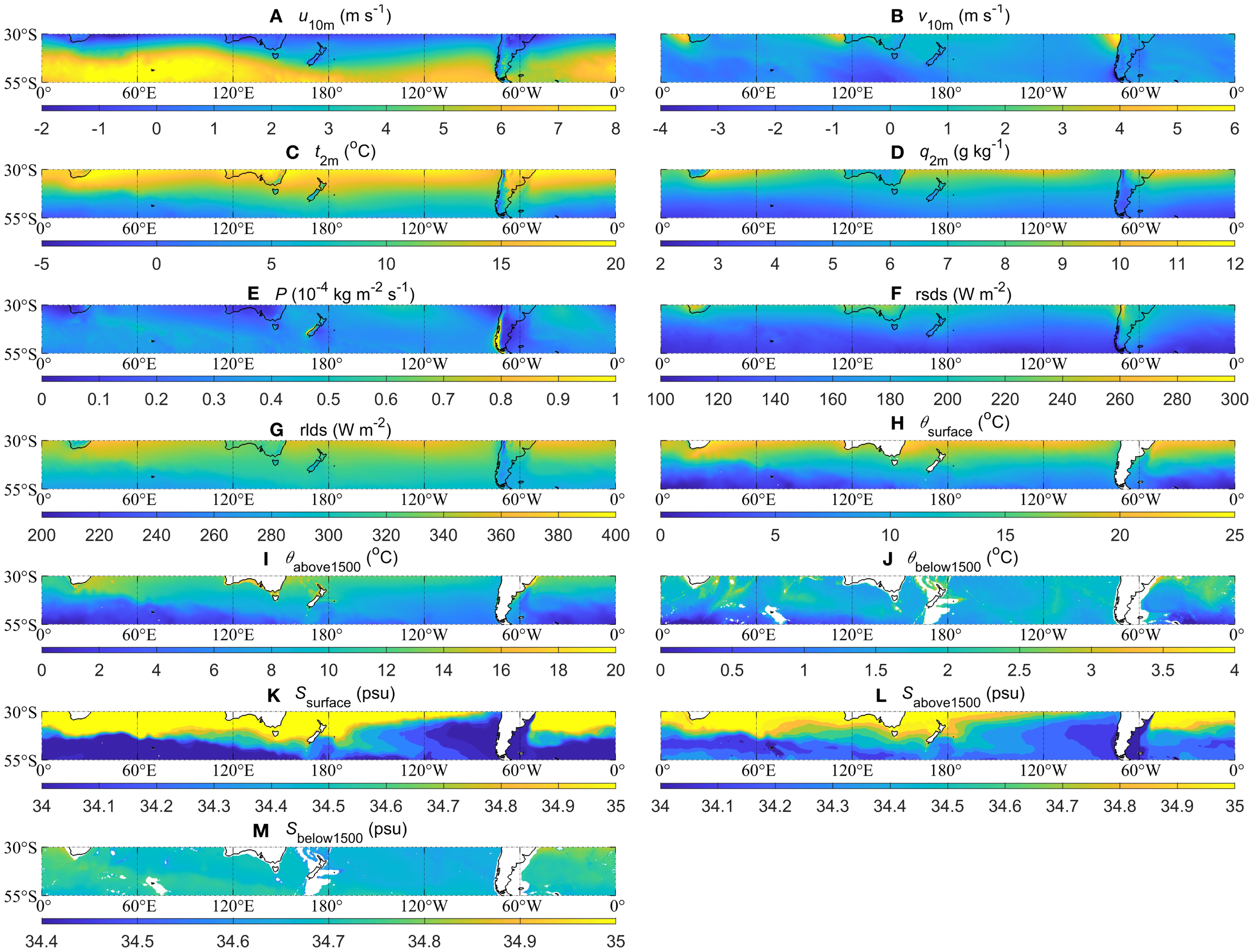
Climatological annual mean of the reference data sets. (A-G) The climatological annual (1940-2023) mean derived from ERA5: (A)u10m (m s-1), (B)v10m (m s-1), (C)t2m (°C), (D)q2m (g kg-1), (E)P (kg m-2 s-1), (F) rsds (W m-2), and (G) rlds (W m-2). (H-M) The climatological annual (1955-2022) mean derived from WOA23: (H)θsurface (°C), (I)θabove1500 (°C), and (J)θbelow1500 (°C); (K-M) similar to (H-J) but for S (psu).
The climatological mean of θsurface is higher around 30°S, typically exceeding 20 °C, and gradually decreases southward (Figure 1H). In the 50°S, θsurface approaches 0 °C. The climatological mean of θabove1500 ranges from 0 °C to 15 °C in most regions in the STZ (Figure 1I), while θbelow1500 is colder (Figure 1J). The spatial distribution of Ssurface and Sabove1500 in the STZ also exhibits noticeable meridional gradients (Figures 1K, L). As latitude increases, the climatological annual mean of Ssurface and Sabove1500 decreases, whereas the spatial gradient of Sbelow1500 is much weaker (Figure 1M).
Figure 2 shows the difference between the CMIP6 MME climatological mean and the climatological mean of two reference datasets (ERA5 and WOA23). The CMIP6 ESMs show stronger biases in westerlies (Figures 2A, B), with intensified west and north winds in the ESMs. The CMIP6 MME mean overestimates u10m by 0.5-1.5 m s⁻¹ over the STZ, particularly in the Indian Ocean sector and the southern Australian ocean. Meanwhile, the CMIP6 MME mean overestimates the negative v10m by 0.5–1 m s⁻¹ in most areas of the STZ. In terms of t2m, a cold bias of 1-2 °C dominates the simulated 2 m air temperature across most ocean surface at 30-45°S (Figure 2C). At 45-55°S, there is a warm bias of ~1 °C in the Indian and Atlantic Oceans (Figure 2C). In the STZ region, q2m is generally overestimated by about 1-1.5 g kg-1 in the CMIP6 simulations, while an underestimation occurs in the South American continent (Figure 2D). In the north of 40°S, the CMIP6 ESMs show a negative bias in the simulated climatological annual mean of P, whereas P generally presents a positive bias in the south of 40°S (Figure 2E). The biases of the rsds are generally opposite to that of the rlds bias (Figures 2F, G). The rsds shows an overestimation in the north of 40°S and an underestimation in the south (Figure 2F), while the rlds shows an opposite spatial distribution (Figure 2G). This result shows reasonable concordance with Xu et al. (2022). Xu et al. (2022) evaluated the simulated rlds by comparing the CMIP6 simulation results with CMIP5 results and ground measurements and identified the positive biases of rlds at 40-55°S.
Figure 2
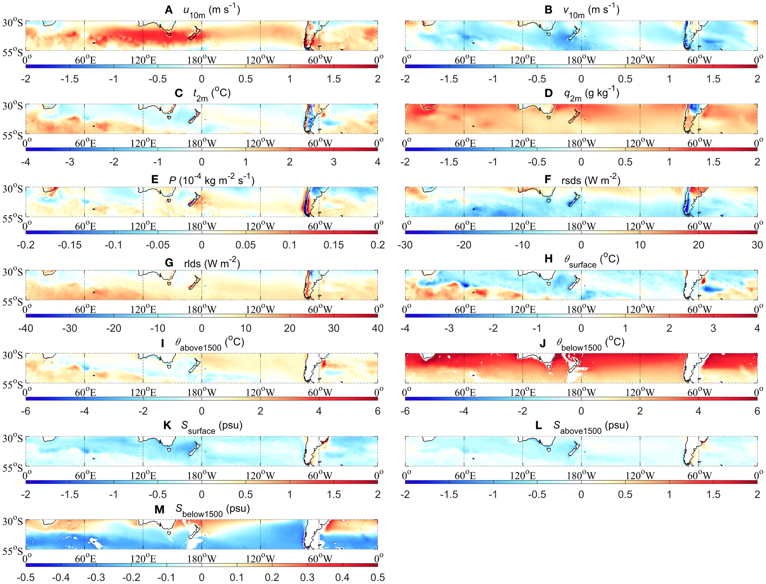
Similar to Figure 1, but for the differences of climatological mean between the MME mean and the reference data (MME mean minus the reference data). (A)u10m (m s-1), (B)v10m (m s-1), (C)t2m (°C), (D)q2m (g kg-1), (E)P (kg m-2 s-1), (F) rsds (W m-2), and (G) rlds (W m-2). (H-M) The climatological annual (1955-2022) mean derived from WOA23: (H)θsurface (°C), (I)θabove1500 (°C), and (J)θbelow1500 (°C); (K-M) similar to (H-J) but for S (psu).
The oceanic fields reveal pronounced thermal biases: the MME mean underestimates the θsurface by 1-2 °C at 40-55°S but shows 1-2 °C warm anomalies at 30-40°S (Figure 2H). In terms of θabove1500, the CMIP6 ESMs overestimate θ by 1-2 °C across most of the STZ ocean (Figure 2I). However, the simulated θbelow1500 is grossly overestimated by CMIP6 MME (Figure 2J). At 30°S, this warm deviation approaches 5 °C (Figure 2J). On the contrary, the simulated climatological annual mean of Ssurface and Sabove1500 shows a clearly fresh bias (Figures 2K, L). In terms of Sbelow1500, the fresh bias between the CMIP6 MME mean and reference data is still very large (Figure 2M).
These biases underscore the substantial discrepancies in the CMIP6 MME mean across variables. Indeed, the magnitude of biases between the CMIP6 MME mean and reference data may remarkably depend on the region analyzed.
3.2 Inter-model spread among CMIP6 ESMs
The SDESM (Equation 1) can serve as a metric to quantify the dispersion of CMIP6 ESMs outputs relative to their MME mean. The inter-model spread, quantified by the SDESM across CMIP6 simulations (Figure 3), highlights significant uncertainty in the near-surface atmospheric fields and the oceanic θ and S. The u10m shows maximum variability over the ACC region, reflecting divergent simulations of westerly jet intensity (Figure 3A). The v10m and t2m fields exhibit similar patterns with respect to the inter-model spread (Figures 3B, C), and their SDESM are generally smaller than 1 m s-1 and 1.5 °C across most regions in the STZ, respectively. In terms of q2m, CMIP6 ESMs show a greater inter-model spread at 30-40°S, especially in the coastal region (Figure 3D). Relatively larger inter-model spread of P is identified at the western Andes in South America and the western side of the New Zealand Island (Figure 3E). Compared to other variables, the rsds and rlds fields exhibit consistently higher inter-model SDESM values in CMIP6 ESMs (Figures 3F, G), underscoring systemic challenges in radiative fluxes. The inter-model spread of θsurface is less than 2 °C (Figure 3H), except for the region of the Brazil Current on the eastern side of South America. In terms of the inter-model spread of θabove1500 and θbelow1500, the CMIP6 ESMs exhibit similar spatial patterns, with a greater spread in 30-45°S, and the Southern Indian Ocean, and a relatively small spread in 45-55°S (Figures 3I, J). The distribution of the SDESM of S exhibits distinct spatial patterns in different layers: larger values of the SDESM are concentrated in subtropical regions (30-40°S) at the surface layer (Figure 3K), while there is a relatively larger inter-model spread over 45-55°S below 1500 m depths (Figure 3M). At the upper 1500 m depth, the SDESM of Sabove1500 is relatively small (Figure 3L). The maximums of the SDESM of Sabove1500 are still around the South American continent (Figures 3K-M).
Figure 3
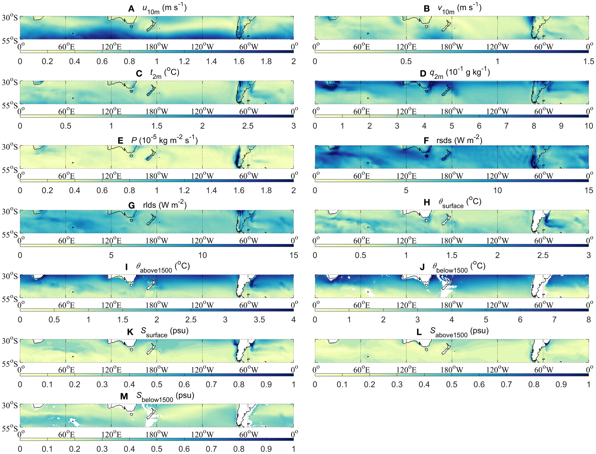
Similar to Figure 1, but for the SDESM among 17 CMIP6 ESMs. (A)u10m (m s-1), (B)v10m (m s-1), (C)t2m (°C), (D)q2m (g kg-1), (E)P (kg m-2 s-1), (F) rsds (W m-2), and (G) rlds (W m-2). (H-M) The climatological annual (1955-2022) mean derived from WOA23: (H)θsurface (°C), (I)θabove1500 (°C), and (J)θbelow1500 (°C); (K-M) similar to (H-J) but for S (psu).
Based on the inter-model spread analysis of CMIP6 ESMs, significant discrepancies still exist among simulations of these key fields. These inter-model spreads underscore persistent systematic challenges in representing the near-surface atmospheric fields, sea fields, and air-sea coupling interactions in the ESMs.
3.3 Ability of CMIP6 ESMs in simulating the climatological annual mean
As discussed in sections 3.1 and 3.2, there are notable discrepancies between the CMIP6 ESMs and the reference data, and the inter-model spread is identified in the simulated multiple variables from the CMIP6. To further analyze the simulation ability of the CMIP6 ESMs, in this section, we employ the MVIE method to systematically evaluate the individual CMIP6 ESMs in simulating multiple variables. Our evaluation focuses on the nine variables specified in section 2.1, encompassing both near-surface atmospheric fields and three-dimensional oceanic fields (denoted by θ and S fields at varying depths).
The VFE diagram uses the RMSL, RMSVD, and VSC to offer comprehensive statistics on the abilities of the ESMs, including the differences between various ESMs and the differences between ESMs and reference data. Figure 4 provides a straightforward intercomparison of 17 CMIP6 ESMs by evaluating their simulated climatological annual mean vector fields that represent all variables.
Figure 4
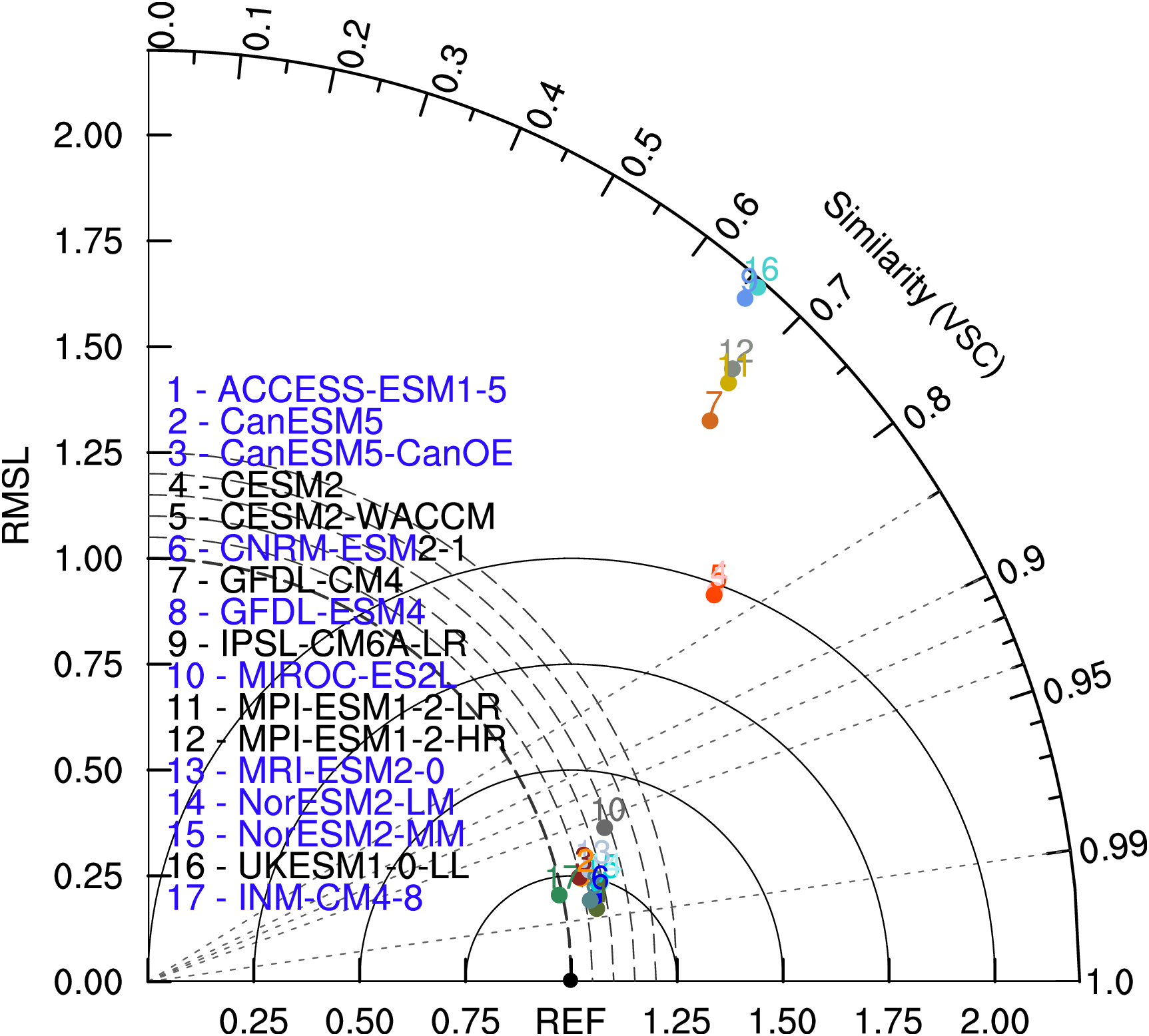
Normalized uncentered VFE diagram of climatological annual mean vector field. The azimuthal position gives the VSC, the radial distance from the origin indicates the RMSL, and the distance between the model and the reference point denotes the RMSVD. The RMSL and the RMSVD are normalized by the RMSL derived from reference data. Different colors and ID numbers represent different CMIP6 ESMs, and the matching relationship between the number and the mode is shown in the legend. The reference data is represented by ‘REF’ (the black point). The blue names of ESMs denote that the differences of the RMSL between the ESMs and reference data are less than 0.5.
In the VFE diagram, the model ability can be diagnosed by the RMSVD between the model and reference data, with a smaller distance from the REF (the black reference point in Figure 4) suggesting a good representation of an ESM. A smaller RMSVD is usually associated with a higher VSC and an RMSL approaching 1. The statistics, such as RMSVD, VSC, and RMSL, of 10 ESMs (the blue names in Figure 4) are close to the reference data, indicating that the differences between these 10 ESMs products and the reference data are relatively small over the STZ region. The VSCs of the 10 ESMs (the blue names in Figure 4) range from 0.94 to 0.99, suggesting that these ESMs can reproduce the spatial pattern of the near-surface atmospheric fields and the oceanic θ and S, with the best estimation from the ACCESS-ESM1-5. The normalized RMSLs of the 10 ESMs are generally larger than 1, indicating that these ESMs tend to overestimate the simulated climatological annual mean vector fields, with the best estimation from the INM-CM4-8.
In contrast, the VSCs of the rest 7 ESMs (the black names in Figure 4) range from 0.6 to 0.85, implying great differences in the spatial patterns of the climatological annual mean vector field between the ESMs products and the reference data. In addition, these 7 ESMs also greatly overestimate the amplitude of the climatological annual mean vector field. Furthermore, we also used the centered VFE diagram to evaluate the anomaly vector fields (Supplementary Figure S2), and the results of model evaluation are similar to those derived from the climatological annual mean vector fields.
The VFE diagram provides insights into the model abilities of ESMs by the VSC and RMSL. To show the performance of ESMs in detail, we further assess more statistical metrics (Figure 5). In addition, we calculated the cMISS to show the multivariable integrated skill, which takes the cVSC and SD into account together. The metrics table adopted the centered statistics that decompose the original fields into anomaly and mean fields. Evaluations of anomaly fields are conducted from three perspectives: the variance characteristics (SD, cRMSL), the spatial pattern consistency (CORR, cVSC), and the root-mean-square differences between the reference data and ESMs results (cRMSD, cRMSVD). The ME is also incorporated in Figure 5 to show the systematic biases of the simulated original fields of ESMs from the reference data.
In terms of the simulated spatial pattern of t2m, q2m, rsds, rlds, and θsurface, the CMIP6 ESMs generally show relatively good performance, with CORRs higher than 0.9. In contrast, with CORRs ranging from 0.1 to 0.9, the CMIP6 ESMs cannot match closely with the spatial pattern of P, θbelow1500 and S from the reference data. It is not easy for these ESMs to adequately reproduce the spatial pattern of θ and S in the deep ocean. Nonetheless, some models still perform relatively well, including CanESM5, CanESM5-CanOE, GFDL-ESM4, and MRI-ESM2-0, with CORRs larger than 0.8. Most ESMs can capture the spatial patterns of the u10m and v10m, yet CORRs of winds from four models are lower than 0.9, including MIROC-ES2L, MRI-ESM2-0, NorESM2-LM, and INM-CM4-8. To derive a comprehensive estimation of the ESMs in simulating the spatial pattern of fields in the STZ, we calculated the cVSC to evaluate the overall performance. The GFDL-ESM4 model shows the highest cVSC (~0.939) among the 17 CMIP6 ESMs, indicating that this model is the most consistent with the reference data in simulating the spatial pattern of the near-surface atmospheric fields and the oceanic θ and S in the STZ region.
The CMIP6 ESMs exhibit considerable differences in simulating the spatial SD of the different fields. For instance, most ESMs tend to overestimate the spatial variability of 10 m vector wind, with 11 out of 17 CMIP6 ESMs overestimating both u10m and v10m over the STZ region. In terms of the spatial variability of q2m, most ESMs tend to have an overestimation by 1%-35%, while the MIROC-ES2L, MPI-ESM1-2-LR, and INM-CM4–8 models tend to have an underestimation by 3%-9%. In terms of the spatial variability of θbelow1500 and Sbelow1500, characterized by an SD larger than 2, some CMIP6 ESMs have a significant overestimation, including the ACCESS-ESM1-5, CESM2, CESM2-WACCM, GFDL-CM4, IPSL-CM6A-LR, MPI-ESM1-2-LR, MPI-ESM1-2-HR, NorESM2-LM, NorESM2-MM, UKESM1-0-LL, and INM-CM4–8 models. In terms of t2m, P, rlds, θsurface, and Ssurface, most CMIP6 ESMs overestimate the spatial variability, whereas the simulated rsds tends to be systematically underestimated. Yet, the SD values of these fields are smaller than 2. As the total SD across all selected fields, the value of the normalized cRMSL larger (smaller) than 1 denotes that the ESM overestimates (underestimates) the anomaly field’s amplitude error. Most ESMs have overestimations, whereas the CNRM-ESM2–1 and MIROC-ES2L models have underestimations. Although the INM-CM4–8 model overestimates the spatial variability of Sbelow1500, it is in most agreement with the reference data, with the cRMSL approaching 1.
The CMIP6 ESMs also show remarkable diversity in simulating the ME of different variables, with ME ranging from -9.2 to 19.9 (Figure 5). Apart from IPSL-CM6A-LR and MIROC-ES2L, with the ME ranging from -0.22 to -0.02, most CMIP6 ESMs overestimate u10m over the STZ. These stronger biases are consistent with the differences between the MME mean and the reference data (Figure 2A). Conversely, apart from the IPSL-CM6A-LR model, most CMIP6 ESMs underestimate v10m, which is in agreement with the broad negative values in Figure 2B. For t2m, the ME of CESM2 has the minimal absolute value that approaches 0, whereas the MIROC-ES2L model has the largest maximum up to 0.297. The INM-CM4–8 model captures the minimum ME of P, while the MIROC-ES2L model tends to overestimate the ME of P mostly. In terms of q2m, the CMIP6 ESMs all tend to have overestimation as indicated by the positive ME. Indeed, the ME values of the near-surface atmospheric fields are all less than 1, implying the relatively good agreement with the reference data. In contrast, the θ and S in the CMIP6 ESMs show relatively larger biases in the ME, especially in the θbelow1500 and Sbelow1500. The θsurface and Ssurface still match well with the reference data, except for the INM-CM4–8 model with the ME of S up to -1.188. In terms of θabove1500 and Sabove1500, the ME values of the CESM2, CESM2-WACCM, and INM-CM4–8 models are larger than 1. Twelve ESMs show strong biases in simulating the θbelow1500, whereas the ACCESS-ESM1-5, MRI-ESM2-0, NorESM2-LM, NorESM2-MM, and INM-CM4–8 models still can have the ME values of θbelow1500 less than 1. Similarly, thirteen ESMs show strong biases in simulating the Sbelow1500, whereas the ACCESS-ESM1-5, CanESM5, CanESM5-CanOE, and CNRM-ESM2–1 models can be close to the Sbelow1500 of the reference data, with the ME values less than 1. The VME measures the differences between two vector fields, and the ACCESS-ESM1-5, CanESM5, CanESM5-CanOE, CNRM-ESM2-1, GFDL-ESM4, NorESM2-LM, NorESM2-MM, and INM-CM4–8 models have relatively smaller VME, with the values less than 0.5.
The statistics of cRMSD are similar to those of ME (Figure 5). The cRMSD values of the near-surface atmospheric fields are also less than 1, indicating statistical agreement with the reference data. The θsurface, θabove1500, Ssurface, and Sabove1500 still match well with the reference data, with the cRMSD values all less than 1. Akin to the ME values, the CMIP6 ESMs exhibit larger values of the cRMSD for the oceanic θbelow1500 and Sbelow1500. Most ESMs show strong differences in anomaly fields between the simulations and the reference data in the abyssal ocean, whereas the cRMSD values of θbelow1500 and Sbelow1500 of the CanESM5, CanESM5-CanOE, CNRM-ESM2-1, and MRI-ESM2–0 models are still less than 1. The cRMSD of multiple fields is measured by the cRMSVD, which indicates the overall difference of the anomaly field in terms of the near-surface atmospheric fields and the oceanic θ and S. Among the CMIP6 ESMs, GFDL-ESM4 has the minimal cRMSVD (0.367), indicating the smallest overall error of multiple anomaly fields.
On the whole, there is no CMIP6 ESM that performs best in every simulated field. The cRMSVD provides an overall evaluation of the model performance, with a smaller RMSVD value corresponding to a better consistency between the CMIP6 ESM and the reference data. However, improvements in the model performance may not always be associated with a monotonically decreasing RMSVD (Huang et al., 2019; Xu et al., 2017). Therefore, the values of the cMIEI and cMISS are computed to provide an overall evaluation that is monotonically associated with the model performance (Figure 5).
Figure 5
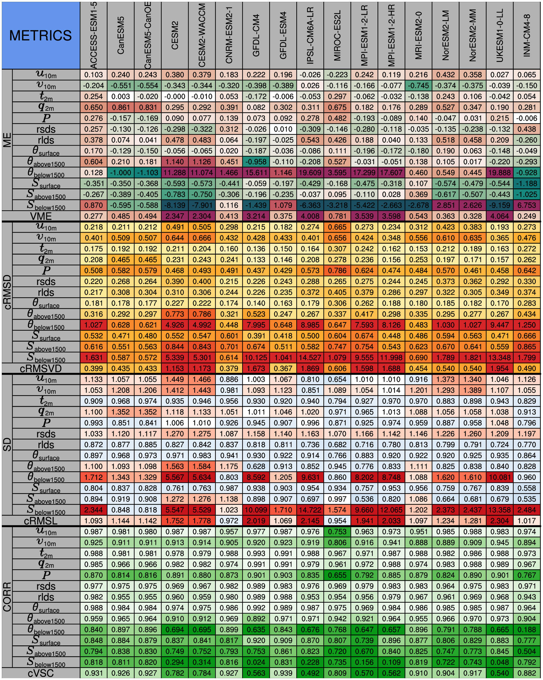
Statistical metrics measuring the abilities of CMIP6 ESMs in simulating the climatology annual mean vector field. VME (ME) quantifies the mean error of the multivariable (scalar) fields. cRMSVD (cRMSD) measures the overall difference in multivariable (scalar) anomaly fields between the CMIP6 ESMs and reference data. cRMSL (SD) and cVSC (CORR) assess the amplitude and pattern similarity of the anomaly fields for the multivariable field (individual field). The SD, cRMSD, and ME are normalized by dividing by the SD of the reference data. The darker colors represent results that are far from the reference data, and vice versa. Warm and cold colors indicate that the biases are larger and smaller than the reference data, respectively.
In order to assess the overall simulation capability for the near-surface atmospheric fields and the oceanic θ and S, we further focus on the values of the centered MIEI and MISS of the 17 CMIP6 ESMs in the STZ region (Figure 6). A better model performance is indicated by a smaller value of the cMIEI and a larger value of the cMISS. We define two benchmark thresholds for a quantitative evaluation: (i) the ESMs with cMIEI < 1 exhibit better simulation skill with respect to the climatology annual mean vector field (including the ACCESS-ESM1-5, CanESM5, CanESM5-CanOE, CNRM-ESM2-1, GFDL-ESM4, MIROC-ES2L, MRI-ESM2-0, NorESM2-LM, NorESM2-MM, and INM-CM4-8); (ii) the ESMs with cMISS > 0.9 exhibit better simulation skill (including the ACCESS-ESM1-5, CanESM5, CanESM5-CanOE, CNRM-ESM2-1, GFDL-ESM4, MRI-ESM2-0, NorESM2-LM, and NorESM2-MM).
Figure 6
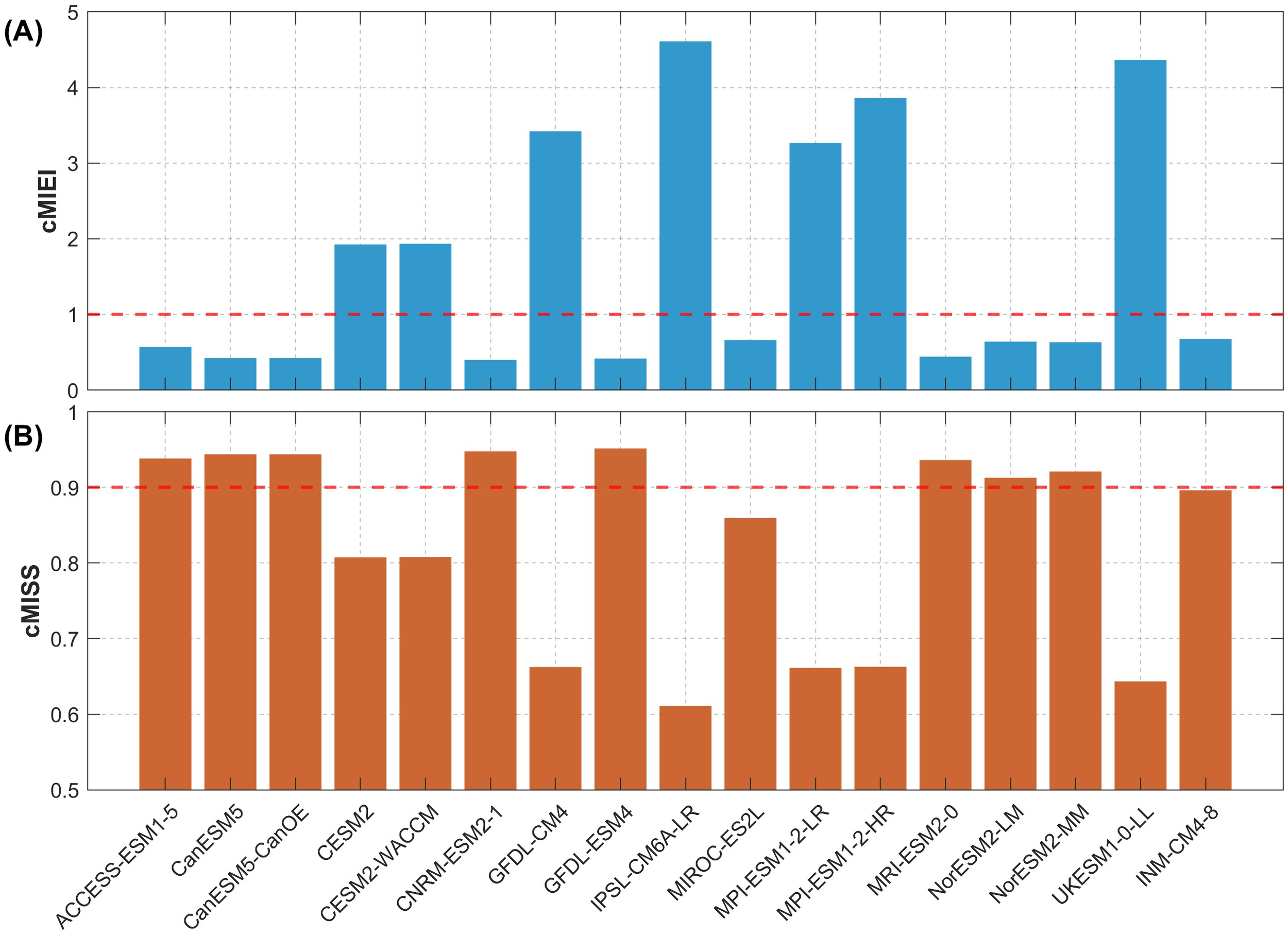
(A) cMIEI and (B) cMISS values for 17 CMIP6 ESMs in the STZ region, measuring the abilities of CMIP6 ESMs in simulating the vector field of climatology annual mean. The dashed red lines denote two selected thresholds for the cMIEI and cMISS, respectively.
The cMISS is an advance over the cMIEI in the reduced sensitivity to amplitude errors, yet we still provide the values of cMIEI for a reference. Based on these two indices, the model performance of the CMIP6 ESMs evaluated is generally consistent, except for the MIROC-ES2L and INM-CM4-8. Finally, eight ESMs (including the ACCESS-ESM1-5, CanESM5, CanESM5-CanOE, CNRM-ESM2-1, GFDL-ESM4, MRI-ESM2-0, NorESM2-LM, and NorESM2-MM) satisfy both criteria, suggesting their better representation of the near-surface atmospheric fields and the oceanic θ and S in the STZ.
3.4 Ability of CMIP6 ESMs in simulating the seasonal climatology
Notable discrepancies of climatological annual means between the CMIP6 ESMs and reference data have been discussed above. Since there is a strong seasonality in the near-surface atmospheric fields and the oceanic θ and S in the STZ (Supplementary Figure S3), a quantitative evaluation of the simulated seasonal climatology could also provide insights into the ESMs ability. Based on the classification of four seasons (DJF, MAM, JJA, SON) described in section 2.2, we further compare the CMIP6 ESMs with the reference data across seasons. Note that our assessments of the seasonality exclude the oceanic θ and S below 1500 m depth because the monthly climatology data of WOA23 only provides data in the upper 1500 m layers.
To compare the performance of various CMIP6 ESMs in reproducing multivariable fields in different seasons, Figure 7 illustrates the VFE diagram of the climatological seasonal means with multiple statistics. The VSCs of all ESMs are larger than 0.95, suggesting that these ESMs can properly replicate the spatial patterns for near-surface atmospheric fields and oceanic θ and S in different seasons. In contrast, the normalized RMSLs generally exceed 1 across seasons, indicating that most ESMs tend to overestimate the vector fields of climatological seasonal means. According to the differences of the RMSL between the ESMs and reference data, the ESMs have better representation in the austral summer (13 ESMs with blue names) and lowest model ability in the austral winter (4 ESMs with blue names).
Figure 7
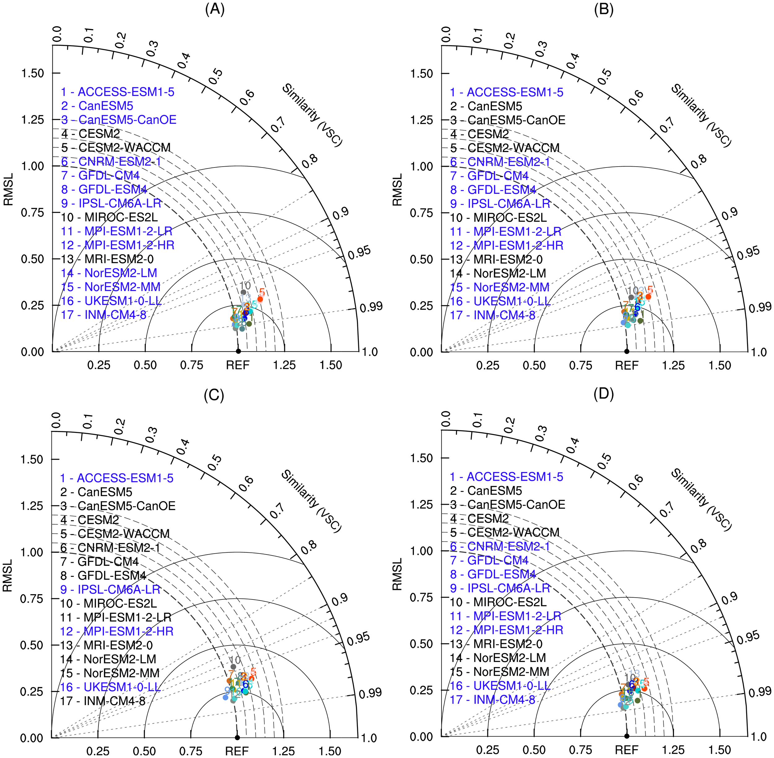
Similar to Figure 4, but for the vector fields of climatological seasonal mean. (A) the climatological seasonal mean during the austral summer (December, January, and February), (B) Similar to (A), but for the austral autumn (March, April, and May), (C) Similar to (A), but for the austral winter (June, July, and August), and (D) Similar to (A), but for the austral spring (September, October, and November). The blue names of ESMs denote that the differences of the RMSL between the ESMs and reference data are less than 0.25.
In stark contrast to the VSCs of the climatological annual mean (Figure 4), the VSCs are mostly improved in the ESMs seasonal products (Figure 7), implying better representations of the spatial patterns of the ESMs seasonal products. The better representation of the seasonal evaluation should be attributed to the exclusion of the oceanic θ and S in the deeper layer, indicating that the oceanic θ and S in the deep layer have larger uncertainties than in the upper layer in the CMIP6 ESMs. We have used the centered VFE diagram to evaluate the anomaly vector fields of seasonal climatology (Supplementary Figure S4), with the outcomes closely resembling those obtained from the uncentered VFE diagram.
The VFE diagrams preliminarily show the model abilities of ESMs through the VSC and RMSL metrics across all four seasons. To delineate the capacity of these models in detail, the 17 CMIP6 ESMs are compared with the reference data. We conduct the comparison by evaluating the VME (ME), cRMSVD (cRMSD), cRMSL (SD), and cVSC (CORR) of the seasonal climatology of the near-surface atmospheric fields and the oceanic θ and S (Figures 8, 9; see Supplementary Figures S5-S8 in the Supplementary Material for the quantitative values in detail). Consistent with the annual assessment, these metrics also employ the centered statistics decomposing seasonal fields into anomaly and mean components.
Figure 8
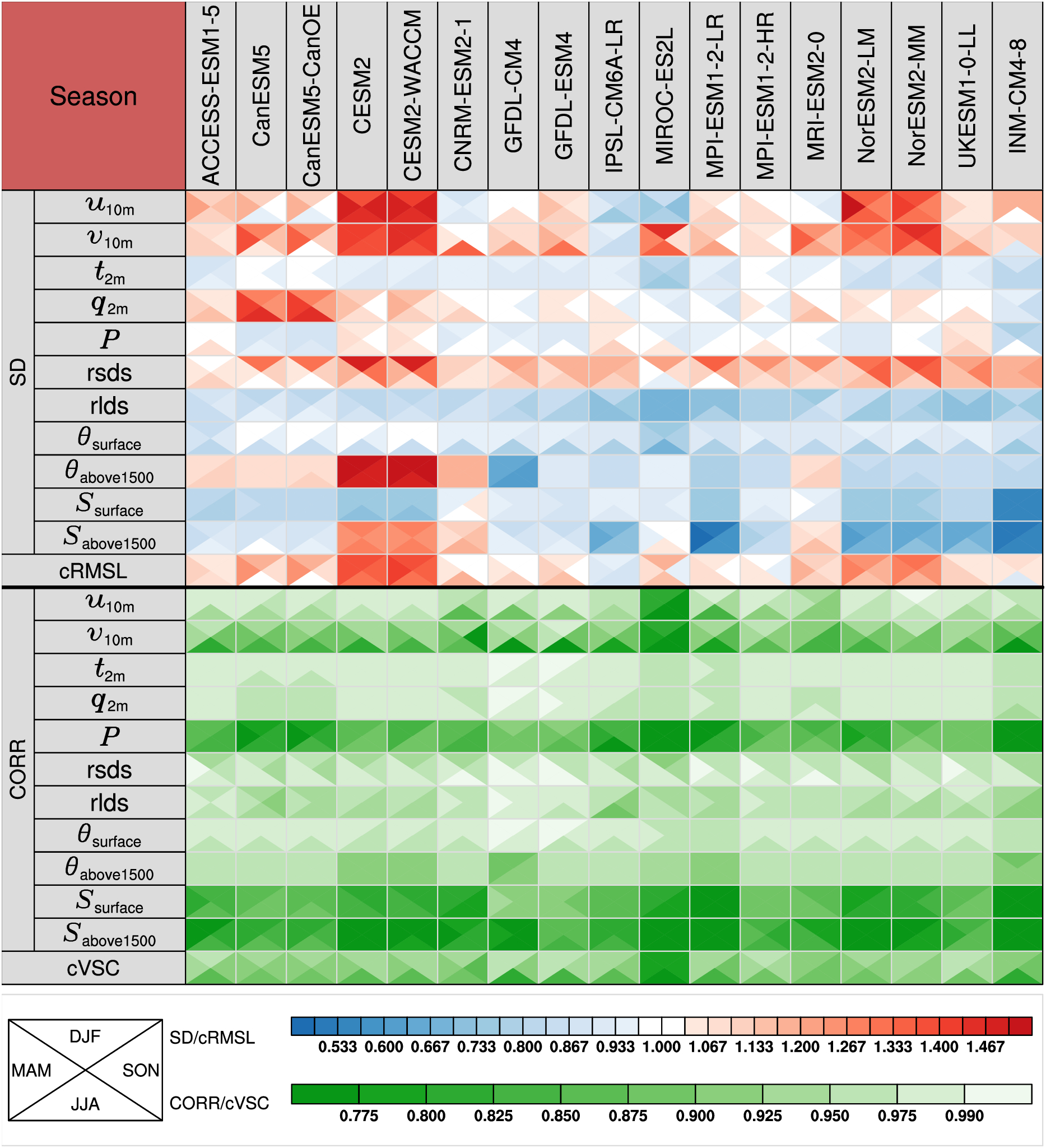
Similar to Figure 5, but measures the abilities of CMIP6 ESMs in simulating the seasonal climatology. As shown in the bottom-left legend, each square is divided into four triangles representing the ESM performance in different seasons. Below the table are shown the colored bars for different statistical metrics.
Figure 9
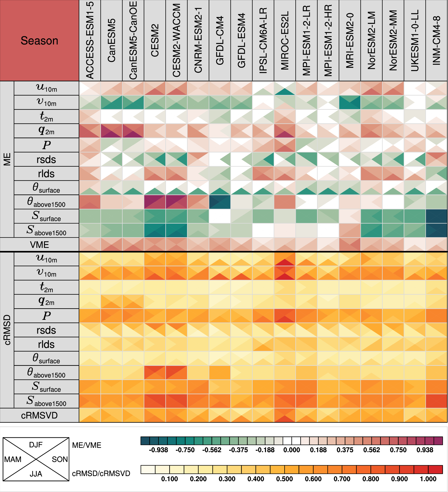
Similar to Figure 8, but for the ME and cRMSD.
Considerable differences have been identified among the CMIP6 ESMs in the simulated spatial SD of different fields and seasons (Figure 8). Across all seasons in the STZ region, a larger number of models, 10 of 17 CMIP6 ESMs, tend to overestimate the variability of 10 m winds. In terms of the spatial variability of q2m, most ESMs also tend to have an overestimation by 2%-45% in the austral summer, autumn, and winter. The CanESM5 and CanESM5-CanOE models both exhibit overestimations up to 45% in winter. In contrast, most CMIP6 ESMs have a better representation of q2m in spring. Most CMIP6 ESMs underestimate the spatial variability of t2m, rlds, θsurface, and Ssurface fields across all seasons, with the lowest estimation of Ssurface by the INM-CM4-8, while the simulation of rsds field tends to be systematically overestimated. Most CMIP6 ESMs can properly capture the spatial SD of P in different seasons. In terms of the spatial variability of θabove1500 and Sabove1500, the CESM2 and CESM2-WACCM models exhibit significant overestimation across all seasons. In contrast, the MPI-ESM1-2-LR and INM-CM4–8 models show a significant underestimation in simulating the Sabove1500. With cRMSL larger than 1, most ESMs have overestimation across all seasons, whereas the IPSL-CM6A-LR models have underestimations throughout the year. Since the CESM2 and CESM2-WACCM models have relatively larger overestimations of the spatial variability of u10m, v10m, and θabove1500, these two models have the largest cRMSL in the austral autumn, with values of 1.392 and 1.409, respectively.
For the simulated spatial pattern of t2m, q2m, rsds, rlds, θsurface, and θabove1500, the CMIP6 ESMs generally exhibit good performance across four seasons, with CORRs typically exceeding 0.9 (Figure 8). In contrast, in terms of the simulated spatial pattern of P, Ssurface, and Sabove1500, the CMIP6 ESMs show relatively poorer performance in reproducing the spatial pattern of the reference data, exhibiting CORRs between 0.5 and 0.9. While reproducing oceanic S spatial patterns remains challenging for the CMIP6 ESMs, several models, including the CanESM5, CanESM5-CanOE, GFDL-ESM4, IPSL-CM6A-LR, MPI-ESM1-2-HR, and UKESM1-0-LL show relatively good performance, with the CORRs of S exceeding 0.8 across all seasons. While most ESMs can capture the spatial patterns of the u10m and v10m during the austral summer, the MIROC-ES2L exhibits a poor wind pattern similarity with the winds of the reference data across all seasons, with the CORRs lower than 0.9. To comprehensively assess the simulated spatial patterns of the ESMs in the STZ, we calculate the cVSC metric for an overall performance evaluation. The MIROC-ES2L model shows the lowest cVSC among the 17 CMIP6 ESMs across four seasons. Most CMIP6 ESMs exhibit relatively poorer performance in simulating the spatial pattern of the near-surface atmospheric fields and the oceanic θ and S during the austral winter, with cVSC generally lower than 0.9.
Remarkable diversity exists among the CMIP6 ESMs in simulating the ME of different variables across different seasons (Figure 9). Most CMIP6 ESMs overestimate u10m over the STZ across four seasons, except for IPSL-CM6A-LR and MIROC-ES2L. In contrast, most CMIP6 ESMs underestimate v10m across four seasons, with the lowest value of -0.774 from the MRI-ESM2–0 in spring, except for the IPSL-CM6A-LR, MIROC-ES2L, and INM-CM4–8 models. Most CMIP6 ESMs have a good representation of t2m and P in simulating the ME across seasons. Yet, the MIROC-ES2L model has a relatively large estimation of the ME of P across all seasons. The ME of q2m and rlds, are generally overestimated in most CMIP6 ESMs, whereas the rsds in most CMIP6 ESMs shows negative biases in the ME. The ME of θsurface of all the CMIP6 models shows negative biases in the austral winter. In terms of Ssurface, the MPI-ESM1-2-LR, MPI-ESM1-2-HR, and NorESM2-MM models match well with the reference data, with the absolute values of ME less than 0.1 across all seasons. In terms of both Ssurface and Sabove1500, most CMIP6 ESMs exhibit underestimation as indicated by the negative ME values, while the INM-CM4–8 model shows relatively poor performance with the ME values less than -1 across all seasons. Measuring the differences between two vector fields, the VME metric shows that the MPI-ESM1-2-HR model has the minimum VME value in the austral summer, autumn, and winter, while the UKESM1-0-LL model has the minimum VME value in the austral spring.
The statistics of cRMSD exhibit similar results to the estimation of ME (Figure 9). During the austral summer, autumn, and winter, the values of cRMSD of the near-surface atmospheric fields and the oceanic θ and S are all less than 1, indicating relatively good agreement with the reference data. Yet, the MIROC-ES2L model shows relatively poor performance in simulating the u10m, v10m, and P, with the values of cRMSD larger than 0.95 in winter. Among the CMIP6 ESMs, the GFDL-ESM4 model has the minimal cRMSVD (0.242 and 0.308) in the austral summer and autumn. The MPI-ESM1-2-HR model has the minimal cRMSVD (0.361 and 0.472) in the austral spring and winter. These results indicate that these two models have the smallest overall error of multiple anomaly fields in the corresponding season.
Similar to the evaluation of the climatology annual mean vector field, we further calculate the values of the cMIEI and cMISS. These statistical metrics are used to assess the simulation capability of the 17 CMIP6 ESMs for the near-surface atmospheric fields and the oceanic θ and S in the STZ region in different seasons (Figures 9, 10). Most CMIP6 ESMs show good performance in the austral summer and relatively poor performance in the austral winter (Figure 10A). The MIROC-ES2L model has the maximum values of cMIEI across all seasons, implying a relatively poor performance. The evaluation of cMISS is largely consistent with the results of cMIEI (Figure 10B). Based on the cMIEI and cMISS metrics, GFDL-ESM4 shows the best performance during the austral summer and autumn. MPI-ESM1-2-HR and NorESM2-MM perform best in the austral winter, and MPI-ESM1-2-HR leads in the austral spring. In addition, the original vector fields are also analyzed with uncentered statistical metrics (Supplementary Figures S9-11).
Figure 10
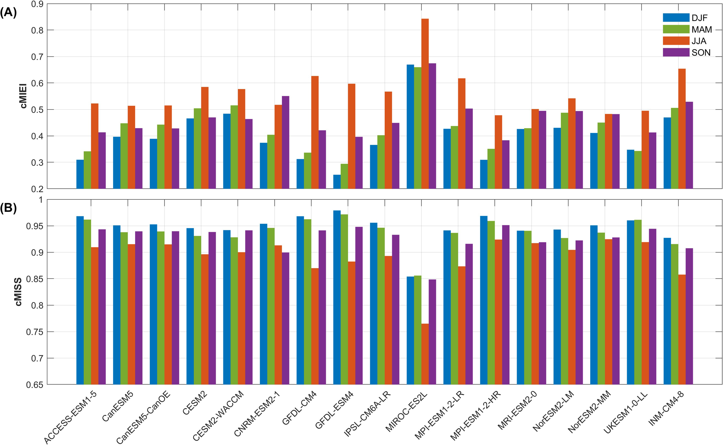
Similar to Figure 6, but measuring the abilities of CMIP6 ESMs in simulating the vector fields of climatology seasonal mean. (A) cMIEI and (B) cMISS values for 17 CMIP6 ESMs in the STZ region. Blue bars represent the austral summer, green bars represent the austral autumn, orange bars represent the austral winter, and purple bars represent the austral spring.
4 Conclusion and discussion
The critical role of air-sea interactions in the STZ, particularly the freshwater and heat fluxes, influences water mass formation and ocean stratification, which in turn affect the global climate (IPCC, 2021). However, the overall performance of the CMIP6 ESMs over the STZ remains unclear. To address this gap, the study aims to provide a comprehensive evaluation of the CMIP6 ESMs over the STZ by using the MVIE method. Unlike previous studies that focused primarily on individual variables, the MVIE method evaluates the multivariable fields as an integrated vector field. Based on the MVIE method, we evaluate the performance of 17 CMIP6 ESMs in reproducing the near-surface atmospheric fields and the oceanic θ and S fields over the STZ region. Eleven variables, including u10m, v10m, t2m, q2m, P, rsds, rlds, θsurface, θabove1500, θbelow1500, Ssurface, Sabove1500, and Sbelow1500, have been introduced as an integrated vector field for the multivariable evaluation. Our systematic evaluation identifies the advantages and limitations of these ESMs in reproducing the near-surface atmospheric fields and the oceanic θ and S fields over the STZ region.
Our evaluation shows that the MME of CMIP6 ESMs shows relatively strong biases in u10m, v10m, q2m, θsurface, θbelow1500, and Sbelow1500 over the STZ relative to the reference data (ERA5 and WOA23). For the atmospheric fields, positive biases of u10m and overestimated negative values of v10m dominate the Indian Ocean and southern Australian sectors, while q2m is overestimated across the STZ region. For oceanic fields, the simulated θsurface shows a zonally banded thermal structure, with cold biases prevalent at 40-55°S and warm biases dominating at 30-40°S in the Indian and Atlantic sectors. This pattern aligns with the warm SST biases in most CMIP6 ESMs, which may be attributed to the adiabatic AMOC transport of deep-ocean heat anomalies from the North Atlantic (Luo et al., 2023). Critically, for deeper ocean layers, θbelow1500 shows pervasive warm biases, while Sbelow1500 exhibits broad fresh biases.
A comprehensive evaluation of 17 CMIP6 ESMs in simulating climatological annual mean fields in the STZ has been conducted. Significant inter-model disparities have been identified in simulating both spatial patterns and amplitudes, with particular challenges for most models in representing θbelow1500 and Sbelow1500 in deeper layers. The GFDL-ESM4 has the best spatial pattern similarity (cVSC closest to 1), while the INM-CM4–8 shows the minimal amplitude bias (cRMSL closest to 1). We find that 10 models, including the ACCESS-ESM1-5, CanESM5, CanESM5-CanOE, CNRM-ESM2-1, GFDL-ESM4, MIROC-ES2L, MRI-ESM2-0, NorESM2-LM, NorESM2-MM, and INM-CM4-8, exhibit relatively good skill in reproducing the integrated climatological annual mean vector field, as indicated by their lower cMIEI values. Furthermore, eight models, including the ACCESS-ESM1-5, CanESM5, CanESM5-CanOE, CNRM-ESM2-1, GFDL-ESM4, MRI-ESM2-0, NorESM2-LM, and NorESM2-MM, consistently rank highest in the integrated skill. These models show both cMIEI < 1 and cMISS > 0.9, signifying relatively better overall representations of the near-surface atmospheric conditions and upper-ocean θ and S fields over the STZ.
To further evaluate the significance of the model rankings, we employed a bootstrap resampling method to show the robustness of our evaluation. The leading models still occupy top positions (Figure 11), including the GFDL-ESM4, CNRM-ESM2-1, CanESM5, CanESM5-CanOE, ACCESS-ESM1-5, MRI-ESM2-0, NorESM2-MM, NorESM2-LM, INM-CM4-8, and MIROC-ES2L models. Although the bootstrap resampling confirms the statistical significance of the superior performance of these models, there are some slight differences between the cMIEI and cMISS rankings. The differences between the cMIEI and cMISS rankings should be attributed to the adjustment of the relative importance between the pattern similarity and amplitude errors in the calculation of cMISS (Zhang et al., 2021).
Figure 11
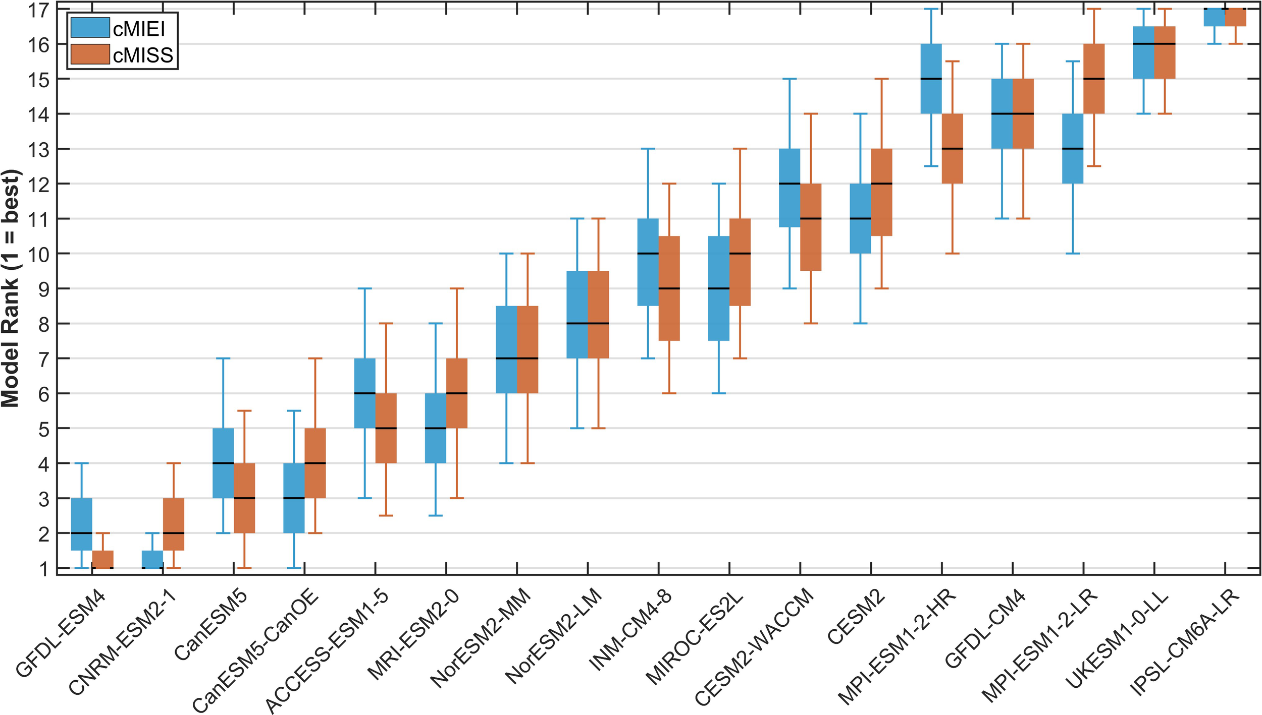
Bootstrap evaluation of the performance of ESMs based on the cMISS and cMIEI values. The boxplots illustrate ranking distributions of 17 CMIP6 models derived from the climatological annual mean (blue color denotes the cMIEI; orange color denotes the cMISS), with rankings obtained through 10,000 bootstrap resampling iterations. Each box represents the interquartile range and median, with the whiskers indicating the 90% confidence interval. Better model performance is indicated by lower rank values (numerically smaller), corresponding to lager cMISS values or lower cMIEI values. Models are ordered along the x-axis by descending cMISS values, positioning better-performing models toward the left side of the figure.
The CMIP6 ESMs also show notable differences in their ability to simulate the seasonal climatology of multiple variables in the STZ. The capabilities of the CMIP6 ESMs show seasonal dependence, with better performance during the austral summer and relatively reduced ability in the austral winter. Compared to the evaluation of the annual mean climatology, the assessments of the seasonal climatology reveal generally improved pattern similarity, suggesting more reliable model representations in the ocean upper layer. The performance of ESMs is sensitive to the vertical depth of the ocean layers involved, with particular biases in θ and S below 1500 m, which may significantly degrade the overall results of evaluation. Overall, the evaluation of the seasonal climatology underscores the importance of better resolving the oceanic θ and S in the deep layer to enhance the ability of ESMs. For the austral winter, the NorESM2-MM and MPI-ESM1-2-HR exhibit the best performance according to the cMIEI and cMISS metrics, while MPI-ESM1-2-HR leads in the spring. During the summer and autumn, GFDL-ESM4 shows better performance. These model rankings are also validated by the bootstrapping method (Supplementary Figures S5-S8).
Furthermore, to analyze potential interrelationships among biases in model variables, we calculated the pairwise correlation coefficients of cRMSD values across the ESMs (Figure 12). These high positive (low negative) correlations suggest that error patterns in these variables tend to co-occur across models: models that perform well in simulating one variable tend to perform well (poor) in the correlated variables, and conversely, models showing large errors in one typically show large (small) errors in the others. We mainly discuss the statistically significant correlations, with CORRs lager than 0.8. The bias of u10m shows a strong positive correlation with v10m, with the CORR of 0.83, indicating that the ESMs exhibiting larger errors in one wind component typically show larger errors in the other. Similarly, model bias in t2m shows particularly strong positive correlations with P, rlds, θsurface, and Ssurface, with the maximum of 0.94 with θsurface. The bias of P has a strong positive correlation with t2m, with the CORR of 0.86. The bias of θbelow1500 shows an extremely high correlation with Sbelow1500 (CORR = 0.99), yet the capability of ESMs in simulating θbelow1500 and Sbelow1500 appears relative independence of other variables. Conversely, the bias of q2m shows no significant correlation with other variables, suggesting that the representation of q2m may operate independently from other examined variables. The CMIP6 ESMs exhibit substantial biases and pronounced inter-model spread in simulating multivariable fields in the STZ region.
Figure 12
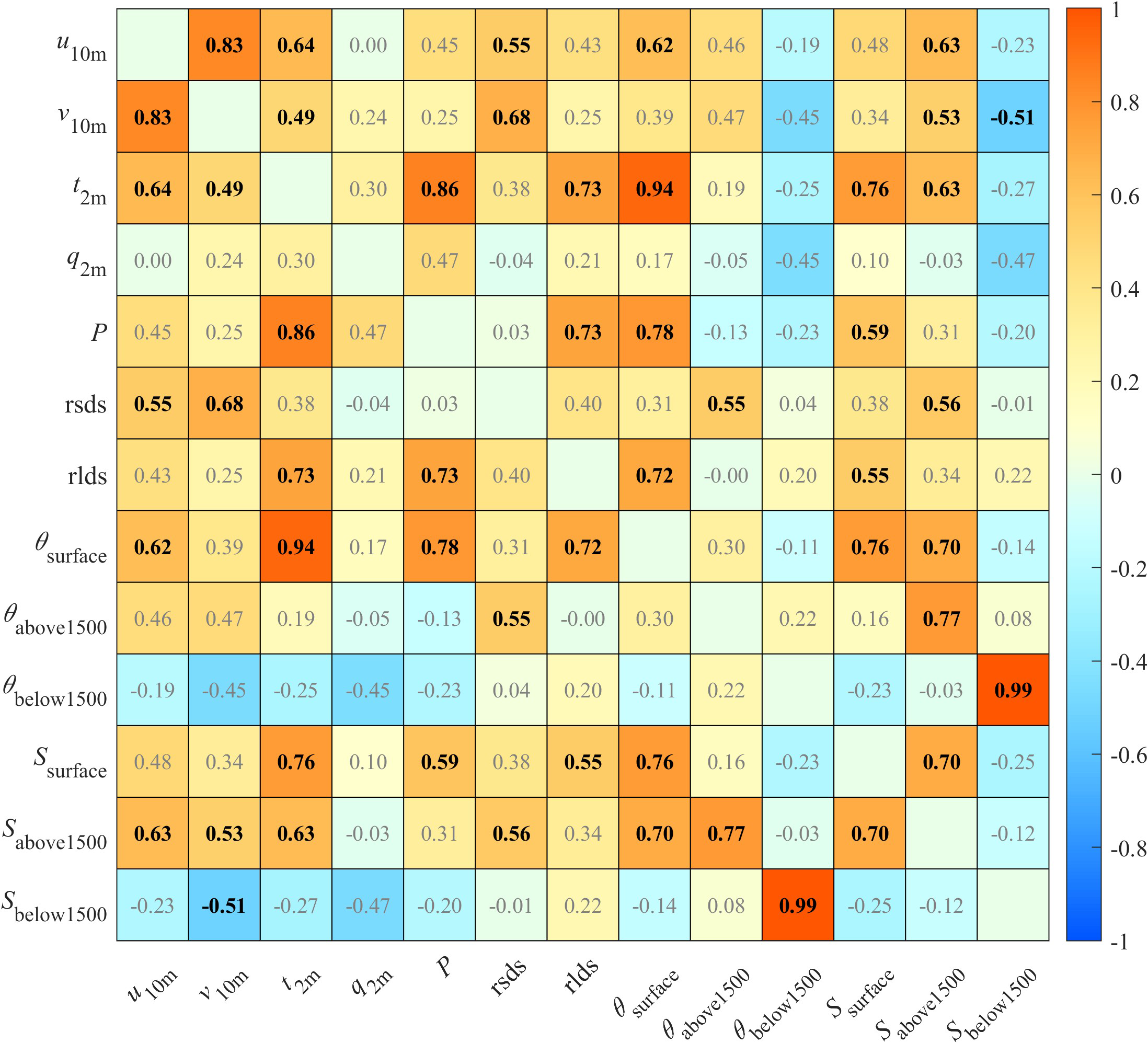
The CORR of cRMSD between pairwise variables of the climatology annual mean across 17 CMIP6 ESMs. Bold black numbers indicate that the CORR between two variables reaches the significance level of 0.05.
The warm and fresh biases in the simulated deep-ocean layers (below 1500 m) of the STZ likely stem from deficiencies in representing some key processes. A primary reason is probably the biased representation of AABW formation (Heuzé, 2021). For many ESMs, AABW forms via open-ocean convection rather than through more realistic shelf processes, leading to insufficient ventilation and incomplete isolation of the abyssal ocean from atmospheric forcing. This can result in an accumulation of heat and a failure to replicate the salinity characteristics in the deep STZ. In addition, remote processes may also contribute to these biases. The adiabatic transport of heat anomalies from the North Atlantic via the AMOC has been proposed as a mechanism for generating Southern Ocean surface warm biases (Luo et al., 2023). It is plausible that this mechanism also influences warming at depth. Moreover, uncertainties in freshwater forcing around Antarctica may contribute to the generation of overly dilute shelf waters (Purich and England, 2021). Such biases can arise from excessive precipitation, unrealistic representations of sea-ice melt and export, or underestimated basal and ice-shelf melt. These freshwater anomalies can alter the density of shelf bottom waters, reducing the efficiency of dense water formation and downslope export, and may therefore lead to the fresh bias that is simulated in the deep Southern Ocean (Purich and England, 2021). More importantly, the relatively coarse resolution in most CMIP6 models cannot adequately represent oceanic mesoscale processes (Hewitt et al., 2020), yet mesoscale eddies are critical for the accurate transport and mixing of heat and freshwater in the Southern Ocean. The influences of mesoscale eddies may not be fully represented through parameterization schemes in most CMIP6 models, and such caveats could introduce biases in the deep ocean. The combination of these local and remote processes may result in a challenge for current ESMs in reproducing the structure of θ and S in the deep region of the Southern Ocean.
This study still has several limitations. First, due to the limited observational data employed in the assimilation of ERA5 and the objective analysis in WOA23, these two reference data sets may still have uncertainties, particularly in the data-sparse Southern Ocean. Second, the three-layer classification of the oceanic fields in this study has not evaluated the thermocline and halocline structures and water masses, respectively. Therefore, a refined vertical discretization aligned with the oceanic mixed layer depth may favor the representation of ESMs in the STZ.
Statements
Data availability statement
The raw data supporting the conclusions of this article will be made available by the authors, without undue reservation.
Author contributions
XP: Investigation, Writing – review & editing, Validation, Methodology, Formal analysis, Writing – original draft, Visualization. CL: Writing – review & editing, Supervision, Investigation, Conceptualization, Funding acquisition. ZW: Writing – review & editing, Supervision, Funding acquisition. ZX: Supervision, Writing – review & editing, Methodology. XLia: Visualization, Writing – review & editing. XLi: Writing – review & editing, Data curation.
Funding
The author(s) declare financial support was received for the research and/or publication of this article. This work was supported by the Independent Research Foundation of Southern Marine Science and Engineering Guangdong Laboratory (Zhuhai) (SML2021SP306, SML2023SP201), the National Key R&D Program of China (2024YFF0506603), the China National Natural Science Foundation (NSFC) Project (42576020), the Natural Science Foundation of Guangdong Province, China (2024A1515012717), and the Southern Marine Science and Engineering Guangdong Laboratory (Zhuhai) (313021004, 313022009).
Conflict of interest
The authors declare that the research was conducted in the absence of any commercial or financial relationships that could be construed as a potential conflict of interest.
The author(s) declared that they were an editorial board member of Frontiers, at the time of submission. This had no impact on the peer review process and the final decision.
Generative AI statement
The author(s) declare that no Generative AI was used in the creation of this manuscript.
Any alternative text (alt text) provided alongside figures in this article has been generated by Frontiers with the support of artificial intelligence and reasonable efforts have been made to ensure accuracy, including review by the authors wherever possible. If you identify any issues, please contact us.
Publisher’s note
All claims expressed in this article are solely those of the authors and do not necessarily represent those of their affiliated organizations, or those of the publisher, the editors and the reviewers. Any product that may be evaluated in this article, or claim that may be made by its manufacturer, is not guaranteed or endorsed by the publisher.
Supplementary material
The Supplementary Material for this article can be found online at: https://www.frontiersin.org/articles/10.3389/fmars.2025.1651187/full#supplementary-material
References
1
Barker P. F. Thomas E. (2004). Origin, signature and palaeoclimatic influence of the Antarctic Circumpolar Current. Earth-Sci. Rev.66, 143–162. doi: 10.1016/j.earscirev.2003.10.003
2
Beadling R. L. Russell J. L. Stouffer R. J. Mazloff M. Talley L. D. Goodman P. J. et al . (2020). Representation of southern ocean properties across coupled model intercomparison project generations: CMIP3 to CMIP6. J. Clim.33, 6555–6581. doi: 10.1175/JCLI-D-19-0970.1
3
Böning C. W. Dispert A. Visbeck M. Rintoul S. R. Schwarzkopf F. U. (2008). The response of the Antarctic Circumpolar Current to recent climate change. Nat. Geosci.1, 864–869. doi: 10.1038/ngeo362
4
Bourgeois T. Goris N. Schwinger J. Tjiputra J. F. (2022). Stratification constrains future heat and carbon uptake in the Southern Ocean between 30°S and 55°S. Nat. Commun.13, 340. doi: 10.1038/s41467-022-27979-5
5
Bracegirdle T. J. Holmes C. R. Hosking J. S. Marshall G. J. Osman M. Patterson M. et al . (2020). Improvements in circumpolar Southern Hemisphere extratropical atmospheric circulation in CMIP6 compared to CMIP5. Earth Space Sci.7 (9), e2019EA001065. doi: 10.1029/2019EA001065
6
Cai W. Gao L. Luo Y. Li X. Zheng X. Zhang X. et al . (2023). Southern Ocean warming and its climatic impacts. Sci. Bull.68, 946–960. doi: 10.1016/j.scib.2023.03.049
7
Chemke R. Ming Y. Yuval J. (2022). The intensification of winter mid-latitude storm tracks in the Southern Hemisphere. Nat. Clim. Change12, 553–557. doi: 10.1038/s41558-022-01368-8
8
Czaja A. Frankignoul C. Minobe S. Vannière B. (2019). Simulating the midlatitude atmospheric circulation: what might we gain from high-resolution modeling of air-sea interactions? Curr. Clim. Change Rep.5, 390–406. doi: 10.1007/s40641-019-00148-5
9
Dai D. Chen L. Ma Z. Xu Z. (2021). Evaluation of the WRF physics ensemble using a multivariable integrated evaluation approach over the Haihe river basin in northern China. Clim. Dyn.57, 557–575. doi: 10.1007/s00382-021-05723-x
10
DeVries T. Holzer M. Primeau F. (2017). Recent increase in oceanic carbon uptake driven by weaker upper-ocean overturning. Nature542, 215–218. doi: 10.1038/nature21068
11
Eyring V. Bony S. Meehl G. A. Senior C. A. Stevens B. Stouffer R. J. et al . (2016). Overview of the Coupled Model Intercomparison Project Phase 6 (CMIP6) experimental design and organization. Geosci. Model. Dev.9, 1937–1958. doi: 10.5194/gmd-9-1937-2016
12
Fahad A. Burls N. J. Strasberg Z. (2020). How will southern hemisphere subtropical anticyclones respond to global warming? Mechanisms and seasonality in CMIP5 and CMIP6 model projections. Clim. Dyn.55, 703–718. doi: 10.1007/s00382-020-05290-7
13
Fogt R. L. Marshall G. J. (2020). The Southern Annular Mode: Variability, trends, and climate impacts across the Southern Hemisphere. WIREs Clim. Change11, e652. doi: 10.1002/wcc.652
14
Frölicher T. L. Sarmiento J. L. Paynter D. J. Dunne J. P. Krasting J. P. Winton M. (2015). Dominance of the southern ocean in anthropogenic carbon and heat uptake in CMIP5 models. J. Clim.28, 862–886. doi: 10.1175/JCLI-D-14-00117.1
15
Gao Z. Zhao S. Liu Q. Long S.-M. Sun S. (2024). Assessment of the southern ocean sea surface temperature biases in CMIP5 and CMIP6 models. J. Ocean Univ. China23, 1135–1150. doi: 10.1007/s11802-024-5808-5
16
Garreaud R. D. Vuille M. Compagnucci R. Marengo J. (2009). Present-day south american climate. Palaeogeogr. Palaeoclimatol. Palaeoecol.281, 180–195. doi: 10.1016/j.palaeo.2007.10.032
17
Goyal R. Sen Gupta A. Jucker M. England M. H. (2021). Historical and projected changes in the southern hemisphere surface westerlies. Geophys. Res. Lett.48, e2020GL090849. doi: 10.1029/2020GL090849
18
Gruber N. Clement D. Carter B. R. Feely R. A. van Heuven S. Hoppema M. et al . (2019). The oceanic sink for anthropogenic CO2 from 1994 to 2007. Science363, 1193–1199. doi: 10.1126/science.aau5153
19
Han Y. Zhang M.-Z. Xu Z. Guo W. (2022). Assessing the performance of 33 CMIP6 models in simulating the large-scale environmental fields of tropical cyclones. Clim. Dyn.58, 1683–1698. doi: 10.1007/s00382-021-05986-4
20
He J. Hong L. Shao C. Tang W. (2023). Global evaluation of simulated surface shortwave radiation in CMIP6 models. Atmospheric Res.292, 106896. doi: 10.1016/j.atmosres.2023.106896
21
Hendon H. H. Thompson D. W. J. Wheeler M. C. (2007). Australian rainfall and surface temperature variations associated with the southern hemisphere annular mode. J. Clim.20, 2452–2467. doi: 10.1175/JCLI4134.1
22
Hersbach H. Bell B. Berrisford P. Biavati G. Horányi A. Muñoz Sabater J. et al . (2023). ERA5 monthly averaged data on single levels from 1940 to present. In: Copernicus climate change service (C3S) climate data store (CDS).
23
Hersbach H. Bell B. Berrisford P. Hirahara S. Horányi A. Muñoz-Sabater J. et al . (2020). The ERA5 global reanalysis. Q. J. R. Meteorol. Soc146, 1999–2049. doi: 10.1002/qj.3803
24
Heuzé C. (2021). Antarctic bottom water and north atlantic deep water in CMIP6 models. Ocean Sci.17, 59–90. doi: 10.5194/os-17-59-2021
25
Hewitt H. T. Roberts M. Mathiot P. Biastoch A. Blockley E. Chassignet E. P. et al . (2020). Resolving and parameterising the ocean mesoscale in Earth System Models. Curr. Clim. Change Rep.6, 137–152. doi: 10.1007/s40641-020-00164-w
26
Hu Y. Tian W. Dong Y. Zhang J. (2024). Evaluating the seasonal responses of southern ocean sea surface temperature to southern annular mode in CMIP6 models. Geophys. Res. Lett.51, e2024GL108782. doi: 10.1029/2024GL108782
27
Huang F. Xu Z. Guo W. (2019). Evaluating vector winds in the Asian-Australian monsoon region simulated by 37 CMIP5 models. Clim. Dyn.53, 491–507. doi: 10.1007/s00382-018-4599-z
28
Huang F. Xu Z. Guo W. (2020). The linkage between CMIP5 climate models’ abilities to simulate precipitation and vector winds. Clim. Dyn.54, 4953–4970. doi: 10.1007/s00382-020-05259-6
29
Hunt G. L. Drinkwater K. F. Arrigo K. Berge J. Daly K. L. Danielson S. et al . (2016). Advection in polar and sub-polar environments: Impacts on high latitude marine ecosystems. Prog. Oceanogr.149, 40–81. doi: 10.1016/j.pocean.2016.10.004
30
IPCC (2021). Climate change 2021: the physical science basis. Contribution of working group I to the sixth assessment report of the intergovernmental panel on climate change. Eds. Masson-DelmotteV.ZhaiP.PiraniA.ConnorsS. L.PéanC.BergerS.CaudN.ChenY.GoldfarbL.GomisM. I.HuangM.LeitzellK.LonnoyE.MatthewsJ. B. R.MaycockT. K.WaterfieldT.YelekçiO.YuR.ZhouX. X. X. B. (Cambridge, United Kingdom and New York, NY, USA: Cambridge University Press). doi: 10.1017/9781009157896
31
Khatiwala S. Primeau F. Hall T. (2009). Reconstruction of the history of anthropogenic CO2 concentrations in the ocean. Nature462, 346–349. doi: 10.1038/nature08526
32
Korhonen H. Carslaw K. S. Forster P. M. Mikkonen S. Gordon N. D. Kokkola H. (2010). Aerosol climate feedback due to decadal increases in Southern Hemisphere wind speeds. Geophys. Res. Lett.37, , L02805. doi: 10.1029/2009GL041320
33
Kushnir Y. Robinson W. A. Bladé I. Hall N. M. J. Peng S. Sutton R. (2002). Atmospheric GCM response to extratropical SST anomalies: synthesis and evaluation. J. Clim.15, 2233–2256. doi: 10.1175/1520-0442(2002)015<2233:AGRTES>2.0.CO;2
34
Levitus S. (1983). Climatological atlas of the world ocean. Eos Trans. Am. Geophys. Union64, 962–963. doi: 10.1029/EO064i049p00962-02
35
Luo F. Ying J. Liu T. Chen D. (2023). Origins of Southern Ocean warm sea surface temperature bias in CMIP6 models. NPJ Clim. Atmospheric Sci.6, 1–8. doi: 10.1038/s41612-023-00456-6
36
Lv M. Xu Z. Yang Z.-L. (2020). Cloud resolving WRF simulations of precipitation and soil moisture over the central tibetan plateau: an assessment of various physics options. Earth Space Sci.7, e2019EA000865. doi: 10.1029/2019EA000865
37
Meehl G. A. Boer G. J. Covey C. Latif M. Stouffer R. J. (2000). The coupled model intercomparison project (CMIP). Bull. Am. Meteorol. Soc81, 313–318. doi: 10.1175/1520-0477(2000)081<0313:TCMIPC>2.3.CO;2
38
Mishonov A. V. Boyer T. P. Baranova O. K. Bouchard C. N. Cross S. Garcia H. E. et al . (2024). World ocean database 2023. C. Bouchard, technical ed. NOAA Atlas NESDIS97. doi: 10.25923/z885-h264
39
Purich A. England M. H. (2021). Historical and future projected warming of antarctic shelf bottom water in CMIP6 models. Geophys. Res. Lett.48, e2021GL092752. doi: 10.1029/2021GL092752
40
Qiu H. Zhou T. Chen X. Wu B. Jiang J. (2024). Understanding the diversity of CMIP6 models in the projection of precipitation over Tibetan Plateau. Geophys. Res. Lett.51, e2023GL106553. doi: 10.1029/2023GL106553
41
Reagan J. R. Seidov D. Wang Z. Dukhovskoy D. Boyer T. P. Locarnini R. A. et al . (2023). World ocean atlas 2023, volume 2: salinity. A. Mishonov, technical editor. NOAA Atlas NESDIS90, 51pp. doi: 10.25923/70qt-9574
42
Rintoul S. Garabato A. (2013). Dynamics of the southern ocean circulation. Int. Geophys.103, 471–492. doi: 10.1016/B978-0-12-391851-2.00018-0
43
Rintoul S. Hughes C. Olbers D. (2001). The antarctic circumpolar current system. Int. Geophys.77, 271-302. doi: 10.1016/S0074-6142(01)80124-8
44
Russell J. L. Dixon K. W. Gnanadesikan A. Stouffer R. J. Toggweiler J. R. (2006). The southern hemisphere westerlies in a warming world: propping open the door to the deep ocean. J. Clim.19, 6382–6390. doi: 10.1175/JCLI3984.1
45
Sanmartín I. Wanntorp L. Winkworth R. C. (2007). West Wind Drift revisited: testing for directional dispersal in the Southern Hemisphere using event-based tree fitting. J. Biogeogr.34, 398–416. doi: 10.1111/j.1365-2699.2006.01655.x
46
Simmonds I. King J. C. (2004). Global and hemispheric climate variations affecting the Southern Ocean. Antarct. Sci.16, 401–413. doi: 10.1017/S0954102004002226
47
Spiridonov V. Ćurić M. (2021). General circulation of the atmosphere. Int. Geophys.229–251. doi: 10.1007/978-3-030-52655-9_15
48
Talukder A. Shaid S. Hwang S. Alam E. Islam K. Kamruzzaman M. (2025). Optimizing the multi-model ensemble of CMIP6 GCMs for climate simulation over Bangladesh. Sci. Rep.15, 11343. doi: 10.1038/s41598-025-96446-0
49
Taylor K. E. (2001). Summarizing multiple aspects of model performance in a single diagram. J. Geophys. Res. Atmospheres106, 7183–7192. doi: 10.1029/2000JD900719
50
Thompson D. W. J. Solomon S. Kushner P. J. England M. H. Grise K. M. Karoly D. J. (2011). Signatures of the Antarctic ozone hole in Southern Hemisphere surface climate change. Nat. Geosci.4, 741–749. doi: 10.1038/ngeo1296
51
Tjiputra J. F. Assmann K. Heinze C. (2010). Anthropogenic carbon dynamics in the changing ocean. Ocean Sci.6, 605–614. doi: 10.5194/os-6-605-2010
52
Wild M. Folini D. Hakuba M. Z. Schär C. Seneviratne S. I. Kato S. et al . (2015). The energy balance over land and oceans: an assessment based on direct observations and CMIP5 climate models. Clim. Dyn.44, 3393–3429. doi: 10.1007/s00382-014-2430-z
53
Xu Z. Han Y. Fu C. (2017). Multivariable integrated evaluation of model performance with the vector field evaluation diagram. Geosci. Model. Dev.10, 3805–3820. doi: 10.5194/gmd-10-3805-2017
54
Xu Z. Hou Z. Han Y. Guo W. (2016). A diagram for evaluating multiple aspects of model performance in simulating vector fields. Geosci. Model. Dev.9, 4365–4380. doi: 10.5194/gmd-9-4365-2016
55
Xu J. Zhang X. Zhang W. Hou N. Feng C. Yang S. et al . (2022). Assessment of surface downward longwave radiation in CMIP6 with comparison to observations and CMIP5. Atmospheric Res.270, 106056. doi: 10.1016/j.atmosres.2022.106056
56
Yang H. Lohmann G. Shi X. Li C. (2019). Enhanced mid-latitude meridional heat imbalance induced by the ocean. Atmosphere10, 746. doi: 10.3390/atmos10120746
57
Yin J. H. (2005). A consistent poleward shift of the storm tracks in simulations of 21st century climate. Geophys. Res. Lett.32, L18701. doi: 10.1029/2005GL023684
58
Zhang M.-Z. Xu Z. Han Y. Guo W. (2021). An improved multivariable integrated evaluation method and tool (MVIETool) v1.0 for multimodel intercomparison. Geosci. Model. Dev.14, 3079–3094. doi: 10.5194/gmd-14-3079-2021
59
Zhang M.-Z. Xu Z. Han Y. Guo W. (2022). Evaluation of CMIP6 models toward dynamical downscaling over 14 CORDEX domains. Clim. Dyn.62, 4475–4489. doi: 10.1007/s00382-022-06355-5
Summary
Keywords
CMIP6 models, Southern Temperate Zone, multivariable integrated evaluation, model bias, model assessment
Citation
Pan X, Liu C, Wang Z, Xu Z, Liang X and Li X (2025) Evaluating the performance of CMIP6 models in the Southern Temperate Zone with a multivariable integrated evaluation method. Front. Mar. Sci. 12:1651187. doi: 10.3389/fmars.2025.1651187
Received
21 June 2025
Accepted
29 September 2025
Published
29 October 2025
Volume
12 - 2025
Edited by
Donglai Gong, College of William & Mary, United States
Reviewed by
Qi Shu, Ministry of Natural Resources, China; Yuanfang Chai, Zhejiang Normal University, China
Updates
Copyright
© 2025 Pan, Liu, Wang, Xu, Liang and Li.
This is an open-access article distributed under the terms of the Creative Commons Attribution License (CC BY). The use, distribution or reproduction in other forums is permitted, provided the original author(s) and the copyright owner(s) are credited and that the original publication in this journal is cited, in accordance with accepted academic practice. No use, distribution or reproduction is permitted which does not comply with these terms.
*Correspondence: Chengyan Liu, liuchengyan@sml-zhuhai.cn
Disclaimer
All claims expressed in this article are solely those of the authors and do not necessarily represent those of their affiliated organizations, or those of the publisher, the editors and the reviewers. Any product that may be evaluated in this article or claim that may be made by its manufacturer is not guaranteed or endorsed by the publisher.