Abstract
Arctic sea ice is highly heterogeneous and composed of a mosaic of different habitats. Our understanding of the impact of climate change on Arctic sea ice and especially on the ice-associated ecosystems is hindered by both a lack of data and a limited understanding of the processes associated with different sea-ice habitats. In particular sea-ice ridges are one of the most under-sampled and poorly understood components of the Arctic sea-ice system. During a spring campaign in the Arctic Ocean, we combined a number of sampling approaches to quantify: 1) the spatial variability of sea-ice algae at single floe and multiple floe scales; 2) the contribution of ridges to ice algal spatial variability; and 3) the role of ridges in shaping the sea ice as a habitat. For upscaling purposes, algal biomass retrieved from ice cores was compared with biomass estimates based on under-ice profiles covering a total of 36 km. Our results show that the level-ice spatial variability measured on a single ice floe can be representative of the larger scale variability. However, only when ridges are included in the analysis we are able to obtain a comprehensive picture of the large-scale ice algal biomass variability. In spring, ridges let more light pass through the ice due to their geometry and their effects on snow distribution, they thus offer a potentially favorable environment for algae to grow within, and they can act as funnels of light for pelagic organisms. On a large scale, ridges contribute more than 50% percent of the potential habitable space for ice algae for snow-covered Arctic sea ice in spring.
1 Introduction
Sea ice in polar regions is characterized by significant variability at many spatial and temporal scales. Such variability remains one of the greatest challenges in sea-ice studies both from an observational perspective and for modeling purposes. Variability in sea-ice physical properties is reflected in the patchiness of sea-ice biogeochemical properties (e.g., Gosselin et al., 1986; Eicken et al., 1991; Granskog et al., 2005; Steffens et al., 2006; Castellani et al., 2020), especially of sea-ice algae (Campbell et al., 2022). Indeed, the variations at different scales support various existing ecological niches. The diverse habitats that sea ice can offer for biological production are still under-sampled, thus assessing the role of sea-ice algal biomass and primary production for polar ecosystems remains a challenge. Lange et al. (2017) showed, based on samples collected during seven ice stations in the central Arctic, that ice core-based estimates of summertime ice algal chlorophyll a (chl a) do not capture the spatial variability resolved by under-ice profiling platforms (Castellani et al., 2020). The above mentioned studies mainly focus on level ice (sea ice which has not been affected by deformation, such a ridging or rafting), however sea ice includes diverse habitats such as meltponds in the Arctic summer, hummocks, ridges, and infiltration layers (e.g., van Leeuwe et al., 2018; Fernández-Méndez et al., 2018).
Pressure ridges are characteristic features of the sea-ice cover in both the Arctic and the Antarctic. They form during sea-ice deformation events, when ice floes collide and create piles of broken ice blocks (called rubble) that extend vertically in the atmosphere and ocean. The portion of ice above the water line is called the sail, and the portion below the water line is called the keel. Typically the rubble has a (macro) porosity of about 30% (e.g. Guzenko et al., 2023), that is voids between the ice blocks filled with air/snow in the sail, or seawater in the keel. Studies using sonar ice draft measurements showed that the fraction of ridged ice in the Arctic can be on the order of 30 to 70% (e.g., Williams et al., 1975; Melling and Riedel, 1996; Hansen et al., 2014; Brenner et al., 2021). The sails and keels affect the interaction of sea ice with the atmosphere (turbulence, accumulation of snow) and with the underlying ocean (drag, accumulation of melt water) (see e.g., Itkin et al., 2018; Castellani et al., 2014; Lu et al., 2011; Castellani et al., 2018; Salganik et al., 2023). After formation, ridges are a loose pile of individual ice blocks that, with time, weather and consolidate due to thermodynamic processes that cause freezing, melt, and refreezing (e.g., Shestov and Marchenko, 2016; Salganik et al., 2023; Lange et al., 2023). The edges of the ridges melt, thus assuming a rounder shape (Kovacs and Mellor, 1971; Høyland, 2002; Wadhams and Toberg, 2012). These changes in the structure of ridges affect their porosity, their strength, and their ability to transmit light. The water-filled voids create habitable spaces for ice-associated organisms. It is this complexity of structure, variable in time and space, that makes ridges a unique sea-ice environment with specific physical characteristics compared to level ice, and thus associated biological processes. The transition to younger, thinner, and more mobile sea ice in the Arctic has resulted in a decline in the proportion of multiyear ice, which typically hosts a greater number of weathered ridges (Maslanik et al., 2007, 2011). At the same time, deformation events have become more frequent in thinner ice, yet this has coincided with a reduction in both the height and density of pressure ridge sails, as recently reported by Krumpen et al. (2025).
Ridges—particularly before melting and consolidation, when they still exhibit high porosity with water-filled voids—have been identified as potential ecological hotspots (e.g., Smetacek et al., 1990; Fernández-Méndez et al., 2018, and references therein). According to Fernández-Méndez et al. (2018), ridge-associated microbes may contribute between 34% and 74% of the total sea-ice biomass, highlighting that ridges not only concentrate biomass but also support distinct microbial communities compared to level ice, thereby increasing biodiversity. Ridges also serve as refugia, feeding grounds, and dispersal platforms for organisms ranging from zooplankton to juvenile fish (Smetacek et al., 1990; Hop and Pavlova, 2008; Gradinger et al., 2010; Gulliksen and Lønne, 1989; Gradinger and Bluhm, 2004; David et al., 2015; 2016). In the Antarctic, ridges have been recognized as an important habitat for the key krill species Euphasia superba (Smetacek et al., 1990; Meyer et al., 2017). However, sampling sea-ice ridges poses significant logistical challenges. Conventional drill-based methods are often difficult and resource-intensive due to the ridges’ structural complexity and large size (Timco and Burden, 1997; Gradinger et al., 2010; Lange et al., 2017). Moreover, the water-filled voids within ridge keels are typically inaccessible using standard sampling techniques. One exception is diver-based sampling, which allows access to the outer flanks of ridges but not their internal voids (e.g., Syvertsen, 1991; Fernández-Méndez et al., 2018). As a result, only a limited number of ridge studies exist with an ecological focus. The few studies to date have mapped ice algal communities (Syvertsen, 1991; Fernández-Méndez et al., 2018) or fauna associated with ridges (Smetacek et al., 1990, Hop and Pavlova, 2008; Gradinger et al., 2010; Gulliksen and Lønne, 1989; Geoffroy et al., 2023; Meyer et al., 2017).
More recently, ridges have been targeted by under-ice profiling and modeling studies. Under-ice profile data has identified ridges as potential hotspots for sea-ice algae compared to the surrounding level ice (Lange et al., 2017, 2024). A recent conceptual modeling study suggests that ridges can be a conduit for light (Katlein et al., 2021) and thus affect light availability for primary producers. For modeling purposes, approaches exist to reproduce ridging events in large scale circulation models and their effect on the atmosphere-ice-ocean coupling (Steiner et al., 1999; Castellani et al., 2018; Martin et al., 2016), in some cases with biogeochemical modeling as focus (Castellani et al., 2017). However, the limited number of studies implies that our understanding of the role of ridges in the sea-ice ecosystem remains fragmentary, making it difficult to draw general conclusions or support large-scale assessments (which are currently based on level-ice observations). Improving our knowledge of ridge contributions is therefore essential for accurately evaluating biological productivity and ecosystem functioning in polar seas.
In the present study we combine different methodologies to conduct a multi-scale comparison of chl a (a proxy for sea-ice algae biomass) in level sea ice and ridges to asses 1) spatial variability of algae from a meter to multi-floe scale to illustrate the effectiveness of traditional ice core sampling; 2) the contribution of ridges to algal spatial variability; and 3) the characterization of ridges and their surrounds with respect to algal habitats. The sampling and the data set used are described in Section 2. Section 3 presents the results obtained that are then discussed in Section 4, followed by concluding remarks in Section 5.
2 Data and methods
2.1 Data
Data were collected during one spring-summer campaign (PS106, May-June-July 2017, Macke and Flores, 2018) on board RV Polarstern (Figure 1). The first part of the campaign (PS106.1) consisted of a drifting ice station, during which Polarstern was anchored to an ice floe for 14 days. Polarstern reached the ice floe located at 81° 57.7’ N, 10° 14.6’ E on June 3rd, and drifted with it until June 16th (Figure 1, thick red track line). Sampling conducted at the drifting ice station included a spatial variability ice coring transect, a ridge coring, and an under-ice survey conducted with a remotely Operated vehicle (ROV; see description in Katlein et al., 2017). During the second part of the campaign (PS106.2) the icebreaker sampled in a region north of Svalbard (Figure 1, maroon track line), conducting sea-ice stations (Figure 1, maroon circles) during one of which another ridge coring took place, and also under-ice hauls using the Surface and Under Ice Trawl (SUIT; Figure 1, yellow circles). The latter allows for large scale sampling of the under-ice environment.
Figure 1
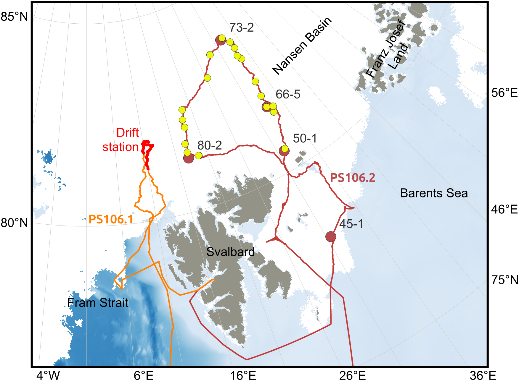
Cruise tracks during the RV Polarstern campaign PS106 superimposed on the sea-ice extent on 25th June 2017 (same date as ice station 45–1 was visited) from AMSR2 (Melsheimer and Spreen, 2019). The drift of the ice floe during PS106.1 between June 3rd and June 16th 2017 is indicated with a thick red line. The ice stations (red circles, see also labels Table 1) and SUIT trawls (yellow circles) are also indicated along the track (maroon line) during PS106.2.
2.1.1 In-situ sampling
2.1.1.1 Ice coring
During the drift station we conducted an in-situ coring study aimed at investigating the spatial variability of sea-ice habitats and associated sea-ice algal biomass, including the contribution of ridges. A transect of ~1200 m was sampled following a (mainly) straight line crossing the ice floe between two sites identified as site A and site B (Figure 2a). A total of 38 cores were extracted with a Kovacs corer (Kovacs Enterprise, Roseburg, OR, United States; inner diameter: 9 cm), all on the same day. At sites A and B, 10 ice cores at each site were taken at 1 m spacing following the nested sampling approach recommended by Miller et al. (2015). Between the two sites, cores were extracted at 100 m spacing. Ice thickness and snow depths were measured at each site where cores were extracted. The bottom 5 cm of each core was sectioned on the field, stored into polyvinyl chloride (PVC) jars and kept in the dark in a cooling box until transported back to the ship. The bottom sections were melted in the dark at +4 °C with the addition of 200 ml of 0.2 mm filtered sea water per 1 cm of ice core (Ehrlich et al., 2020; 2021). Once fully melted, samples were filtered through Whatman GF/F filters. The filters were put into liquid nitrogen and stored at -80 °C on board. After the expedition, when samples returned to the host institute in Germany, pigments including chl a were extracted from the filters with 100% Acetone and homogenized. The chl a concentrations were retrieved by measuring autotrophic pigments using High-Performance Liquid Chromatography (HPLC, for more details, see Tran et al., 2013).
Figure 2
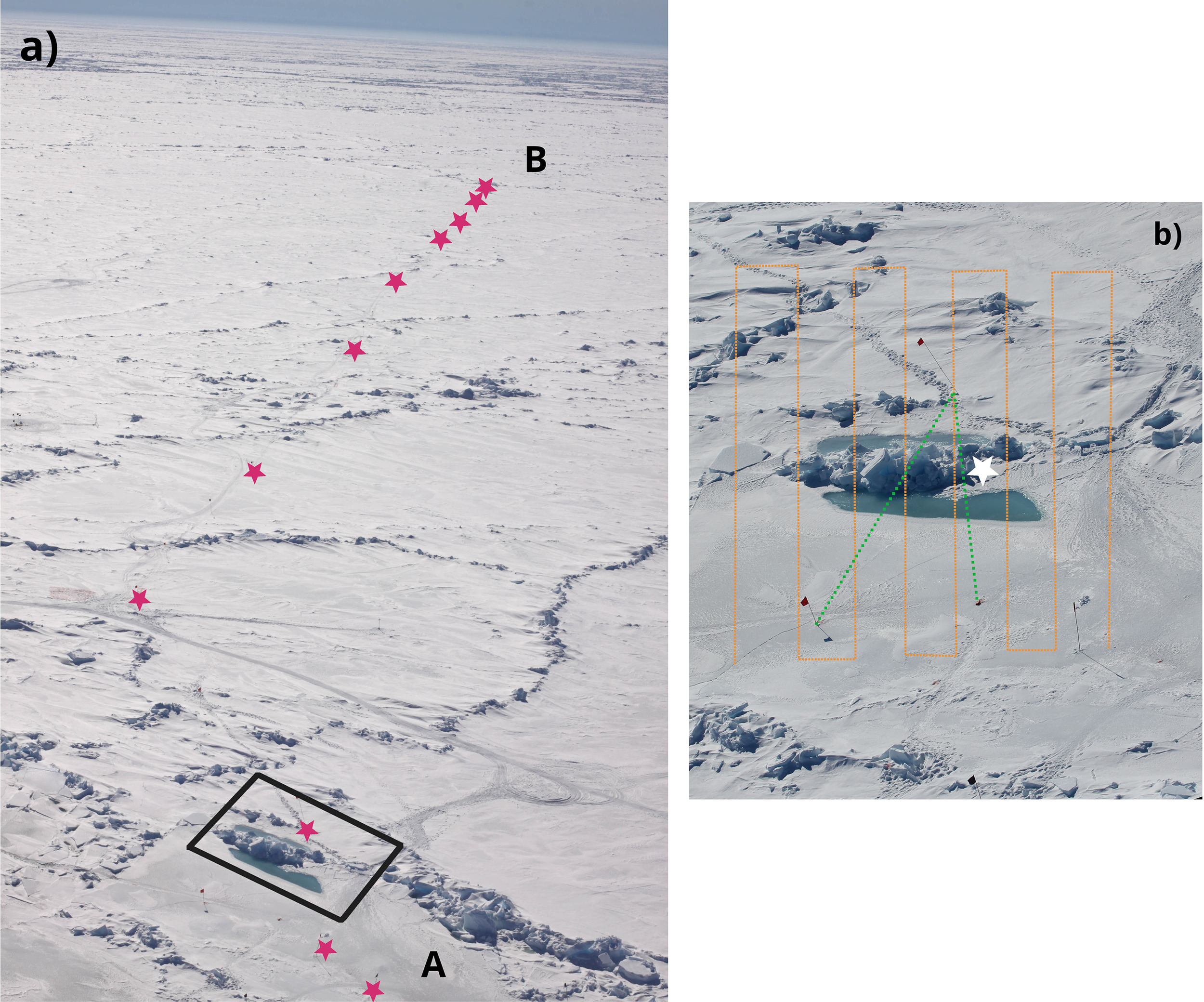
Aerial view of (a) the single-floe spatial variability study, and (b) the ridge study that were conducted at the ice drift station during RV Polarstern expedition PS106.1. The purple stars in a) mark the locations where ice cores were taken. In proximity of sites A and B, 10 cores at each site were collected with 1 m distance. The black box indicates the ridge that was chosen for the ridge study. In (b) the orange lines indicate the approximate location of the under-ice ROV dive. The green line indicates the location of the snow transect. The white star indicates the location of the ridge-specific coring event. Pictures were taken a few days after the ice-core drilling event.
On the same ice floe two cores for chl a analysis were extracted from a ridge crossing the transect (Figure 2b, white star). The ridge was formed due to the collision of a thinner ice floe (hosting site A) with a thicker ice floe (where site B was located). Differently from level ice, where algal communities in the bottom 5 cm usually dominate the total biomass (Tedesco et al., 2025), in ridges ice algae may be vertically distributed due to their complex structure (e.g. Fernández-Méndez et al., 2018). Thus in the case of ridges we sampled, melted, and filtered for chl a analysis a full core.
Five more ice stations were conducted during PS106.2 (see Table 1; Figure 1). At station 66–5 on July 3rd a second ridge was sampled. Further sampling of ridges was limited by logistical constraints related to both the coring process and subsequent sample handling.
Table 1
| Station nr. | Lat (°N) | Lon (°E) | Ice thickness (m) | Snow depth (m) |
|---|---|---|---|---|
| 45-1 | 78.11134 | 30.47859 | 0.90 ± 0.31 | 0.07 ± 0.06 |
| 50-1 | 80.50841 | 30.98369 | 1.15 ± 0.07 | 0.06 ± 0.03 |
| 66-5 | 81.65542 | 32.34167 | 3.09 ± 0.2 | 0.07 ± 0.09 |
| 73-2 | 83.66128 | 31.58055 | 1.37 ± 0.1 | 0.07 ± 0.03 |
| 80-2 | 81.30809 | 16.88646 | 1.15 ± 0.08 | 0.02 ± 0.02 |
List of ice stations sampled during PS106.2 with position, mean ice thickness and mean snow depth (± standard deviation).
2.1.1.2 Under-ice ROV survey
On June 12th (PS106.1) we conducted a survey to map the ridge and adjacent level ice (Figure 2b). A snow depth survey crossing the ridge from site A into the adjacent floe (Figure 2b, green line) was conducted with a GPS-equipped Snow Depth Probe (Magnaprobe, Snow-Hydro, USA). Before conducting the snow depth survey, when the environment was still pristine, under-ice surveys for light transmission and ice draft measurements (Figure 2b, orange line) were conducted with an ROV equipped with a RAMSES‐ACC‐VIS spectroradiometer (TriOs GmbH, Rastede, Germany). Another sensor of the same type measuring incoming radiation above the ice was used to retrieve transmittance (Katlein et al., 2017; 2019). Spectral measurements were integrated over the spectral range of the instruments from 320 to 950 nm. Sea-ice draft was measured by the difference between the ROV depth (pressure) and the distance to the ice determined by an upward looking sonar altimeter. No corrections were applied to the hyperspectral data for the water between the sensors and the ice bottom due to two factors: (1) under-ice blooms were absent (average chl a concentration: 0.59 mg m-3), and (2) a bulk water-column extinction coefficient cannot be reliably defined under a spatially inhomogeneous ice surface (Katlein et al., 2016), especially in areas with ridges where complex geometry increases heterogeneity.
2.1.2 SUIT under-ice profile data
To compare ice core point measurements with variability at the scale of hundreds to thousands of meters, we mapped the sea ice with a Surface and Under Ice Trawl (SUIT, van Franeker et al., 2009; Flores et al., 2012). The SUIT is a net towed behind the ship that maintains contact with the underside of the ice through buoyancy. Its frame is equipped with sensors to monitor sea ice and under-ice properties. A detailed description of the SUIT and the associated dataset can be found in Castellani et al. (2020) and the data are available in Castellani et al. (2019). A detailed schematic of SUIT is presented in Flores et al. (2012) and in Supplementary Figure S1 of the Supplementary Material. Our analysis here focuses on a subset of the data presented in Castellani et al. (2020), in particular: (i) the sea-ice draft for the retrieval of ridges along the transects and for calculating the light field in the ridged and in the level ice; and (ii) the within-ice chl a retrieved by spectral analysis of under-ice light as described in Castellani et al. (2020) for a comparison with the in-situ core sampling (see Section 3.1). The total distance covered by the SUIT hauls during the campaign was 36188 m, with an average ice thickness of 1.91 m (Castellani et al., 2020).
2.2 Identification of ridge keels along the SUIT profiles
Ridges feature a sail extending above the sea level and a keel protruding into the water. As the SUIT provides information on the sea-ice draft, we identified ridge keels along the hauls. Ridge identification was performed by adapting the algorithm based on previous published works which focused either on ridge sails (e.g., Castellani et al., 2014; Krumpen et al., 2025) or ridge keels (Castellani et al., 2015). For a step-by-step explanation of the algorithm see Section S1 in the Supplementary Material. Given a profile of sea-ice draft values from a single SUIT haul, the ridge identification algorithm searched for local maxima (points where the sea ice was thickest) that satisfied a prominence threshold. We set the threshold at 1.5 m below the level ice draft in that haul, as the thickness of the level ice differed based on sampling location and ice characteristics. For a given SUIT haul, the 25th percentile of ice draft value determined the level ice draft, so a topographic element was a potential ridge keel if it exceeded the level ice draft by 1.5 m. For each local maximum that satisfied the depth condition, starting from the largest and progressing in descending order, the Rayleigh criterion (Rabenstein et al., 2010; Castellani et al., 2014, 2015) was applied to determine whether the maximum represented a single ridge keel. According to this criterion, new ridge keels must be separated from previously identified ones by a point that is at least half the maximum depth. For each potential ridge, the left and right extents of the keel were determined by selecting the points at half depth along either side of the keel. We ensured that the width was larger than 5 m. The amount of ridged ice for each detected keel was defined as that portion of ice contained between the left and right extents of the keel. In some cases, a new potential ridge keel overlapped with a previously identified keel, so we resolved the conflict by imposing the following conditions:
-
If one keel’s boundaries completely contained another’s (this can be the case of a small local maximum near a larger one) we kept only the larger keel and its left and right boundaries;
-
Two local minima could conflict because they were both part of a larger ridge with a flat bottom edge. We checked if the mean ice draft between the two minima was greater than 90% of the deeper of the two ridge keels in question. If so, the two minima were merged and we kept the left and right boundaries of the union of the two, otherwise the point with minimum ice draft between them marked the separation between two ridges;
-
In the case that two ridges were separated by just a single point (i.e., only one point between two local minima satisfied the Rayleigh criterion - this was usually due to noise in the data with sudden changes in the thickness e.g., a sudden point of very thin ice compared to the neighboring data points), then the two ridges were merged.
By applying this algorithm, we ensured that there were no overlapping ridges. The applied conditions may not cover all cases for other ice draft datasets. By visual inspection, we found that for the present data set this method identified distinct keel-like features without the need to impose assumptions about their shape and size apart from those listed above. After the identification of ridges, the rest of the sea ice along the profile was assumed to be level ice. It is important to note that the percentage of ridged ice along the transect is affected by the criterion used to define the ridges. An example profile is shown in Figure 3. Median depth and width of the ridges, and median ridge frequency/spacing were computed for each SUIT haul.
Figure 3
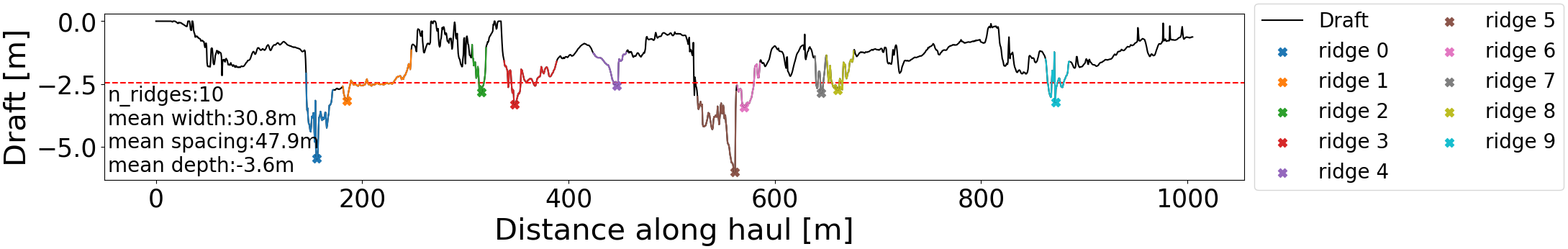
Example of sea-ice draft from SUIT haul 5 (station 66-4) along with identified ridges. The keel of the identified ridges are marked with a colored ‘x’ and the part of the draft belonging to the ridge is highlighted in the respective color. The ice categorized as level ice is plotted with a black line. The red dashed line is the minimum depth required for a local minimum to qualify as a ridge. For this haul, the level ice draft is -0.96 m and thus the keel threshold is -2.46 m.
2.3 Under-ice light field and habitable space
Transmittance T and ice draft zd measured with the ROV along the ridge transect were used to calculate bulk extinction coefficients (κb) for parameterizing light transmission through sea ice (Grenfell and Maykut, 1977) following the approach of Katlein et al. (2019):
with FT being the light transmitted through the ice integrated over the wavelength range, F0 the integrated incident irradiance, i0 the parameter accounting for the absorption in the Surface Scattering Layer (SSL, Castellani et al., 2021; Lebrun et al., 2023), and Hi (m) the ice thickness. In the present we converted ice draft to ice thickness with a correction factor of γ=1.1 (Katlein et al., 2019), and we assumed a value for the surface transmission parameter of i0 = 0.35. Bulk extinction coefficients (m-1) were thus calculated as:
After calculating the bulk extinction coefficients for all the draft points, we separated the ridges from level ice similarly to what was done for the SUIT data (Section 2.2). With this aim we first computed modal thickness along the full ROV transect. We then assigned the label ‘ridge’ to every point that was thicker than the modal thickness plus a threshold value of 1.5 m. The remainder of the transect was considered level ice.
By dividing the sea-ice environment between level and ridged, an extinction coefficient for each of the two environments could be computed. These two different extinction coefficients were then applied to the SUIT ice draft profiles with the aim to quantify the amount of habitable space for sea-ice algae. The habitable space is defined here by the depth limit at which algae still receive enough light as PAR (Photosynthetically Active Radiation, 400–700 nm) to develop a bloom. We note that a bloom is defined as the time when algal growth becomes exponential. The threshold value for light used for ice algal bloom was taken from Stroeve et al. (2024) and Castellani et al. (2017) as 1.78 μmol photons m-2 s-1. It has to be noted that the recent study by Hoppe et al. (2024) reports a value for algal growth of 0.04 ± 0.02 μmol photons m−2 s−1. However, this value was identified as a threshold for initial algal growth at the transition from polar night into spring. Considering that the season of the present study is different from the study of Hoppe et al. (2024) and algae are already acclimated to higher light levels (Michel et al., 1988; Campbell et al., 2015), and since we are interested in algal bloom rather than initial growth, we applied the threshold value from Stroeve et al. (2024). Incoming light for each SUIT haul was computed as in Castellani et al. (2020) as the modeled hourly incoming solar radiation (μmol photons m−2 s−1) above the surface (1°x1° spatial resolution, daily temporal resolution, interpolated hourly) based on the radiative transfer model SBDART (Ricchiazzi et al., 1998) as described in Laliberté et al. (2016). We then inverted Equation 1 to calculate the depth at which the transmitted light remains above the threshold value for an ice algal bloom.
3 Results
3.1 Spatial variability of sea-ice chl a
3.1.1 Ice-core based values
Based on the ice cores extracted along the spatial variability transect, the drift station ice floe had a mean ice thickness of 1.54 m and a mean snow depth of 16 cm. However, there was a significant difference between the two high resolution sites: site A (mean thickness of 0.7 m and mean snow depth of 2 cm) and site B (mean thickness of 1.72 m and mean snow depth of 13 cm). This difference in ice characteristics supports the hypothesis that the floe sampled was created by the convergence between a thicker floe (hosting site B) and a thinner one (hosting site A). This deformation event formed the ridge that was sampled for the ridge study (ice coring and ROV). The full profile showed a large variability in ice thickness and snow depth (Figure 4) with ice thickness values ranging between 0.55 and 3.20 m and snow depths ranging between 0.05 and 0.75 m. The largest ice thickness was measured for an ice core extracted close to the ridge in an area where several ice blocks piled up under the ice. Values of chl a along the entire spatial variability transect remained low and showed a lower variability than the physical parameters. The concentration of chl a varied between 0.12 and 1.2 mg chl a m-2. This range is within the variability measured at both the higher resolution site A (from 0.23 to 0.9 mg chl a m-2) and site B (from 0.01 to 0.67 mg chl a m-2). Ice cores collected during PS106.2 ice stations varied between 0.01 and 1.62 mg chl a m-2, thus remaining in a very similar range of variability as those observed during the drift station.
Figure 4
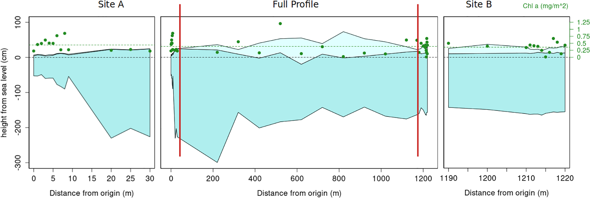
In-ice chl a along the spatial variability transect plotted as green dots on top of the corresponding locations where ice cores were extracted (reference axis on the right side of the panels). The middle panel shows the entire transect (red vertical lines indicate the position along the transect of the site A and B high resolution sampling), the left and right panels are a close-ups of the high frequency sampling sites A and B respectively. The dark blue part represents ice, whereas the light blue is the snow.
3.1.2 SUIT values
Chl a values from the SUIT data were retrieved by applying a Normalized Difference Indices (NDI) algorithm to the under-ice hyperspectral measurements collected with the Trios Ramses sensors mounted on the SUIT (see Castellani et al. (2020) for details). Derived values ranged between 0.00 and 5.77 mg chl a m-², and thus the majority of the values fall in the range of those taken during the ice stations (i.e., Figure 4), but some higher values exceed the in-situ range. A comparison between ice cores and SUIT derived data is shown in Figure 5. In order to establish a floe scale VS multiple-floes scale comparison, we compared the variability of the chl a values along the spatial variability coring transect (Figure 5a, blue dots) and those at the PS106.2 ice stations (Figure 5a, green dots), together with the ridges sampled during both legs (Figure 5a, red diamonds), to the chl a values retrieved along the individual SUIT hauls. The variability covered by the coring transect, as well as that covered by the ice stations during PS106.2, (representing multiple floes) is enough to cover most of the variability measured with the SUIT. However, along hauls 1, 5, 6, and 19 (Figure 5b) the SUIT profiles present larger values (>2 mg chl a m-2) than observed in any ice cores.
Figure 5
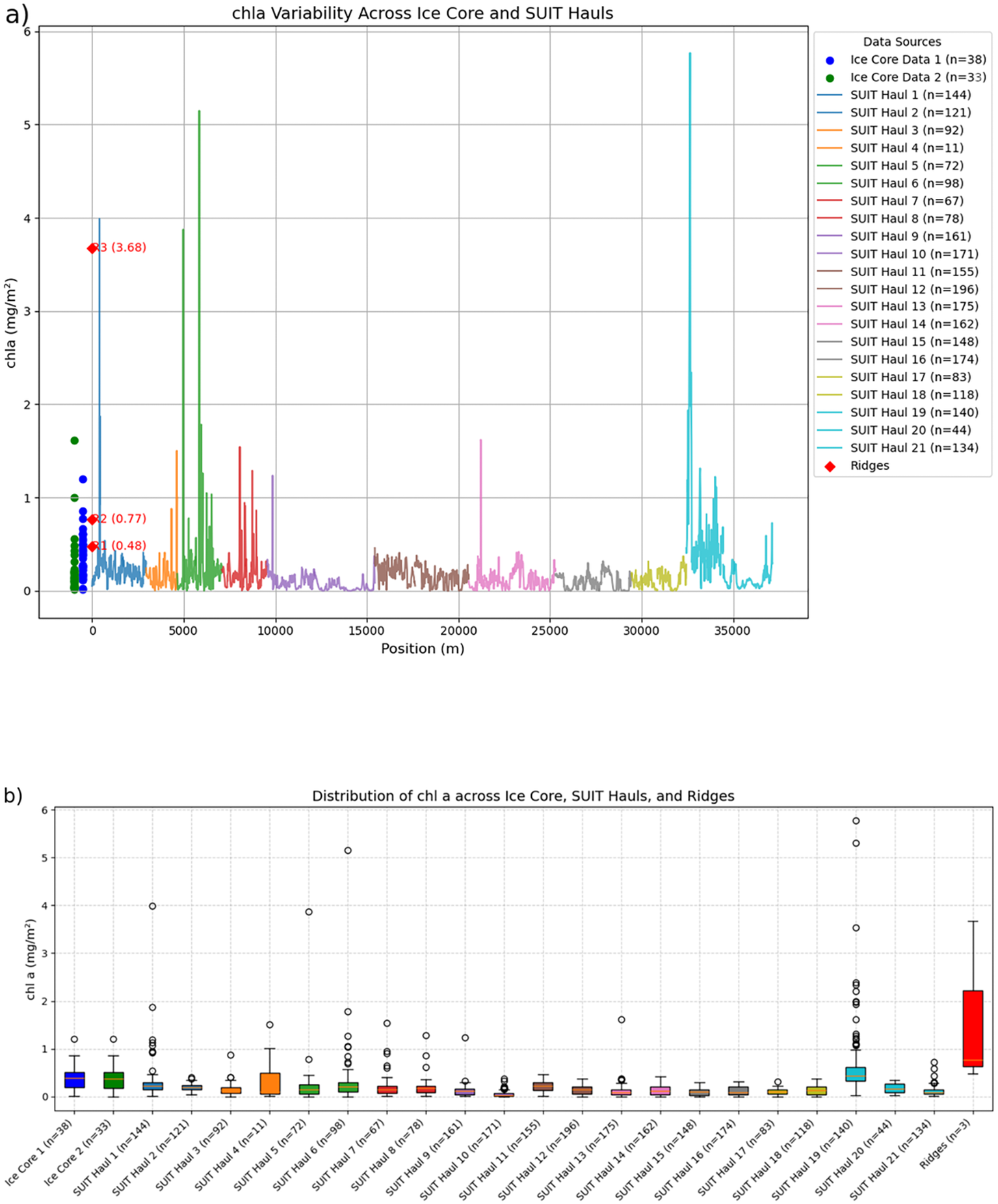
Comparison between chl a retrieved from coring and derived from SUIT under-ice profiles. (a) SUIT under-ice hyperspectral measurements (each profile is plotted as a line of different color to distinguish between the different hauls) and ice cores collected during the spatial variability experiment (blue dots), during the ridge coring (red diamonds), and at the ice stations visited during PS106.2 (green dots). (b) Box-plot of chl a values grouped according to the single-floe spatial variability (Ice Core 1), the ice stations visited during PS106.2 (Ice Core 2), the samples collected from the ridges (Ridges) and all the individual SUIT hauls.
3.2 Ridge characteristics
Chl a in the two samples collected from the ridge along the spatial variability profile was 0.48 mg chl a m-2 and 0.77 mg chl a m-2, respectively. These are within the range of the level ice cores from both PS106.1 and PS106.2. Only the third ridge sample collected at station 66-5 (PS106.2) shows higher in-ice concentration of 3.68 mg chl a m-2.
Along the ROV transect (Figure 6) maximum ridge draft was 3 m. The high heterogeneity in the spatial distribution of draft values (Figure 6b) suggests that the ridge consisted of many separated blocks, as typical for first year (FY) ice ridges. The variability in ice draft is reflected in transmittance, with values ranging from 0.0004 to 0.049, and in bulk extinction coefficients (Figures 6a, c). Extinction coefficients retrieved with Equation 2 are systematically high (> 5 m-1) for low ice thicknesses (Figures 6c, d), whereas for drafts larger than 1.5 m (classified as ridged ice) values are as low as 1.1 m-1. By splitting the ice between level and ridged we obtained an average extinction coefficient of 12.1 m-1 for level ice and of 1.9 m-1 for ridged ice. When considering both ice types together, the mean bulk extinction coefficient was 4.76 m-1. Snow depth across the ridge (Figure 6e) varies between 0 on top (crest) of the ridge and on the side of site A, and 96 cm on the level ice surrounding the ridge on the site B floe.
Figure 6
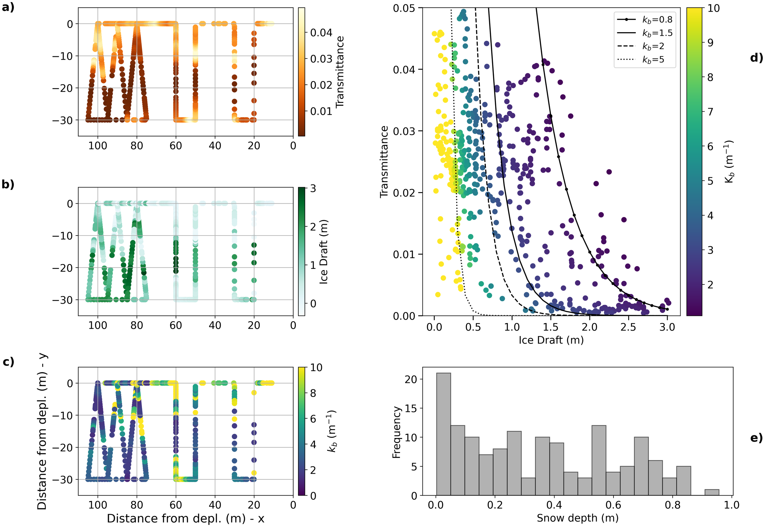
ROV survey of level ice and ridge. The left panel shows: (a) transmittance, (b) ice draft, and (c) extinction coefficient along a transect crossing the ridge multiple times. The x and y axes show the distance from the deployment point of the ROV in a local coordinate system where (0,0) is the deployment position. (d) Scatter plot of ice draft and transmittance together with calculated extinction coefficients (kb), where regressions are shown for different values of extinction coefficients; (e) Snow distribution along a transect crossing back and forth the ridge (Figure 2).
3.3 Large scale contribution of ridges to the sea-ice habitat
We applied the algorithm described in Section 2.2 to retrieve ridge statistics along each SUIT haul. The density of ridges for each SUIT profile is listed in Table 2, whereas Supplementary Figure S2 shows the probability density functions for keel depth, ridge width, and keel spacing for the entire sampling during PS106.2. Apart from haul 20, which is a short haul (626 m), ridges are present in every haul. The depth of the keels peaked at about 3 m and 5 m, with the first peak being in good agreement with what we measured on the drift station ice floe (see Section 3.2). The median keel depth was -3.7 m (mean depth -4.1 m). Maximum keel depth exceeded 8 m in only a few cases, with the deepest keel observed at 14 m. Ridge width also showed a bi-modal distribution with peaks at 20 m and 45 m, with a median width of 28.5 m (mean width 44.5 m). Most ridges were narrower than 100 m, but in a few cases they were as large as 220 m. Such large values can happen e.g., when the algorithm detects a ridged field, so several ridges are merged together. There was no distinct relationship between ridge keel depth and width, which reflects the non-parametric ridge detection algorithm. Spacing between ridges showed large variability with values as low as few meters and as large to exceed 1000 m, with a median spacing of 69 m (mean spacing 141 m). By combining information of ridge width along the transect, we were able to compute the fraction of ridged ice for each SUIT haul (Table 2); as a linear fraction along hauls, about one quarter (24.4%) of the ice is classified as ridged. We note at this point that the percentage of ridged ice is sensitive to the assumption on how the width of a ridge is defined.
Table 2
| Station nr. (haul nr.) | Haul distance (m) | No. ridges | Median keel depth (m) | Median keel width (m) | Median keel spacing (m) | Median level ice draft(m) | Median ridged ice draft (m) | Ridge ice linear fraction (%) |
|---|---|---|---|---|---|---|---|---|
| 50-5 (1) | 1691 | 7 | -3.32 | 16.5 | 57.75 | -0.91 | -3.16 | 9.85 |
| 63-1 (2) | 1309 | 10 | -2.28 | 17 | 39 | -0.78 | -1.93 | 14.67 |
| 65-4 (3) | 2213 | 9 | -4.72 | 69.5 | 202 | -1.84 | -2.37 | 36.74 |
| 66-4 (5) | 1005 | 10 | -3.2 | 26.25 | 74.5 | -1.39 | -2.39 | 30.7 |
| 67-5 (6) | 1466 | 11 | -3.47 | 19 | 46.75 | -0.91 | -1.52 | 21.07 |
| 68-5 (7) | 1320 | 4 | -4.26 | 88.5 | 126.5 | -1.71 | -4.22 | 34.99 |
| 69-2 (8) | 1158 | 8 | -3.98 | 10.75 | 37.5 | -1.11 | -2.52 | 23.09 |
| 70-1 (9) | 2627 | 7 | -3.17 | 152.5 | 202.75 | -1.71 | -2.61 | 40.01 |
| 71-5 (10) | 3304 | 10 | -4.29 | 45 | 70.5 | -2.02 | -2.82 | 25.65 |
| 72-5 (11) | 2218 | 8 | -2.46 | 39.25 | 148 | -0.89 | -1.85 | 14.88 |
| 73-7 (12) | 2948 | 21 | -4.74 | 25.5 | 46 | -1.59 | -2.83 | 21.39 |
| 74-5 (13) | 2494 | 15 | -3.78 | 18 | 80 | -1.32 | -1.83 | 20.61 |
| 75-6 (14) | 2274 | 16 | -3.87 | 38.5 | 108 | -1.59 | -2.15 | 23.35 |
| 76-4 (15) | 2400 | 19 | -4.31 | 35.5 | 55.25 | -1.61 | -2.91 | 28.48 |
| 77-2 (16) | 2014 | 12 | -4.76 | 29.75 | 62.5 | -1.95 | -1.72 | 28.41 |
| 78-5 (17) | 1422 | 10 | -4.34 | 17.25 | 36 | -1.68 | -4.23 | 19.23 |
| 79-1 (18) | 1580 | 9 | -4.33 | 42 | 91.25 | -1.99 | -2.54 | 18.1 |
| 80-3 (19) | 2020 | 10 | -3.51 | 25.5 | 66 | -1.61 | -3.07 | 14.82 |
| 83-7 (20) | 626 | 1 | -4.64 | 149.5 | – | -1.37 | -3.49 | 23.88 |
| 83-8 (21) | 2104 | 10 | -2.91 | 41.75 | 118.5 | -1.37 | -2.2 | 30.31 |
Ridge characteristics for each SUIT haul.
Columns 4, 5, and 6 present the median values for the keels identified. Columns 7 and 8 show the median thickness of the ice classified as ridged and of the level ice. The last column present the percentage of ridged ice along each transect.
Habitable space is defined as the amount of space between the ice surface and a particular depth that offers optimal light conditions for microbial growth. As optimal light conditions we considered the threshold of light for algal bloom onset chosen as 1.78 μmol photons m−2 s−1 (Stroeve et al., 2024; Castellani et al., 2017). Since the extinction coefficient for light in the ridges is lower than in level ice, the habitable space within ridges extends deeper in the ice. We calculated the habitable space in ridged ice and level ice for each SUIT haul in the two cases of maximum and minimum hourly incoming irradiance for each day. An example transect is presented in Figure 7a, where the yellow shading represents the extent of the habitable space, whereas the percentage along each SUIT haul of habitable space in the two different habitats is shown in Figure 7b. The depth at which the light threshold is still met is larger for ridges than for level ice. In some cases, the habitable space would extend further below the ridges in the water column. This implies that ridges can let enough light pass through to trigger a bloom also in the underlying water column. Figure 7b highlights that the contribution of ridges to the habitable space was always larger than that of the level ice, and in some cases the contribution of ridges was more than double.
Figure 7
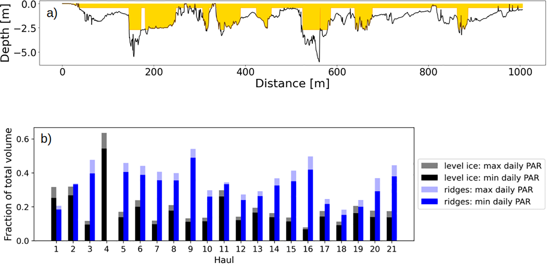
Habitable space in sea ice. (a) Example of habitable space (yellow shading) in the ridged ice and in the level ice along SUIT haul 5 (station 66-4), same as shown in Figure 3. (b) Percentage of habitable space in ridges (blue color) compared to habitable space in level ice (black) for all the SUIT hauls. Habitable space is calculated for the maximum level of PAR per day and for the minimum PAR level.
4 Discussion
4.1 Spatial variability of ice algal biomass
Along the spatial variability coring transect (~1200 m), values of chl a remained quite low everywhere, despite that the light levels were high enough to trigger algal growth and bloom (Hancke et al., 2018; Hoppe et al., 2024). This was true for both those sites characterized by a thick snow cover (especially site B) and those characterized by almost no snow (site A), suggesting that in our case snow was not the only factor controlling algal patchiness. The lack of such a relationship between low chl a and snow depth (Gosselin et al., 1986; Mundy et al., 2005) could be explained by the fact that by the time we reached the ice floe melt had not started yet, thus the snow was not solidified and was still redistributed under the action of the wind. This means that the contribution of different snow depths might have been homogenized and smoothed out by moving snow dunes (Liston et al., 2007). However, without direct measurements of snow redistribution dynamics prior to our sampling, this remains a hypothesis requiring further investigation. Low chl a values could also be due to a decrease in cellular chl a content due to light acclimation (Campbell et al., 2015; 2018), but no algal physiology studies were conducted on these samples, so we have no means to test this hypothesis. The data presented here provide only a snapshot of the biophysical system, and the lack of historical information on the ice and algae constrains our analysis and interpretation. Although light and nutrient availability are key factors controlling ice algal growth, also the past history of the environment e.g., light history (e.g. Galindo et al., 2017), melt and refreeze cycles of the ice (e.g. Yoshida et al., 2020), and ice formation and initial algal incorporation into the ice (e.g., Gradinger and Ikävalko, 1998; Niimura et al., 2000; Kauko et al., 2018; Różańska et al., 2008; Ito et al., 2025) adds to the complexity of algal build-up over time. Further, we know even less about how algae evolve in ridges that have distinctly different habitats (such as water filled voids) than level ice.
The chl a concentrations sampled during the spatial variability coring survey on a single ice floe are in agreement with the values of ice cores collected at other ice stations east and north of Svalbard during the second leg (PS106.2). This shows that the small-scale variability is similar to the large-scale variability and that only one ice floe can be representative of the larger area, if a sufficient number of ice cores is analyzed (Miller et al., 2015). It is difficult to provide a definitive minimum number of ice cores needed, since such numbers may change depending on season and geographical location, but we argue that at least 15–20 ice cores should be collected, ensuring that the spacing between cores varies following a nested design (Miller et al., 2015). With respect to ridges, we collected three ice cores for chl a samples from two locations. Two of the samples were comparable with the concentrations observed in the level-ice cores, however, one ridge had a significantly higher concentration of chl a. This result agrees with previous studies (e.g., Fernández-Méndez et al., 2018; Lange et al., 2017) showing that ridges can be biological hotspots, but not consistently so. More importantly, our results also show that the algal biomass within ridges is more variable than in level ice and ridges need to be included in field sampling if the aim is to collect representative data of sea-ice biomass.
The chl a values retrieved along the SUIT hauls (covering a total of 36 km) contain both level ice and ridged ice. The chl a from ice cores, both along the spatial variability coring transect and those from the ice stations, fall within the range of the SUIT values, however, they do not fully cover the SUIT variability. It is indeed only with the inclusion of ridges that we can really cover the full variability found by the SUIT. This result shows that ridges should be included in estimates of algal biomass if we aim at obtaining a comprehensive idea of the sea-ice biomass on a regional scale. It has to be noted that the within-ice chl a values from the SUIT were obtained by applying an NDI algorithm built on level ice samples only (Castellani et al., 2020), thus the SUIT values could underestimate the actual algal biomass in ridges. Moreover, algal communities may be different between the two environments (e.g. Fernández-Méndez et al., 2018) resulting in different signals in the spectral shape. However, no studies tackling such differences are currently available to correct any possible biases.
4.2 The role of ridges in shaping the ice scape
The mean ridge keel density for the whole SUIT sampling length (~36 km) is 5.5 per km which is in good agreement with what Krumpen et al. (2025) showed for ridge sails the same year 2017 in the Arctic Ocean across the Trans-Polar Drift stream (TPD). The mean spacing between ridge keels of 106 ± 50 m as inferred from the present data is also in good agreement with Krumpen et al. (2025). We can thus conclude that the methodology used here based on an improved algorithm applied to the SUIT under-ice draft profiles is able to capture ridge statistics representatively. There is no possibility to derive ice age from the SUIT data, however, the two peaks in keel depths at 2.5 m and 4.5 m may represent two distinct sea-ice types. From Castellani et al. (2020), their Table 4, we infer that at the stations west of 20°E (hauls 15 to 21) the ice was on average thicker than in the other hauls (in their case there is no distinction between level and ridged ice), which may explain the thicker ridges. Ridged ice accounts for between 10% and 30% of all ice along the SUIT hauls (Table 2). This is in agreement, but on the lower end, with data reported in the literature (e.g., Brenner et al., 2021). We note here that the amount of ridged ice strongly depends on the assumption made for defining the width of the ridges, thus we may introduce a bias when we use the width at half depth compared to e.g., inspecting the profiles by eye and manually identifying the two edges of the ridges relative to adjacent level ice. Another potential bias arises from the ship’s tendency to navigate through thinner, less ridged ice, which may lead to an underestimation of the actual proportion of ridged ice. Moreover, ridges are kinematic linear features that can extend for very long distances compared to their width, so the transects we collected in the present work may not be able to fully capture the total contribution of ridges to the ice scape.
This study presents a quantitative analysis of under-ice profiles collected beneath a ridge using an ROV, providing new insights into how ridge presence can alter the surrounding sea-ice environment. Due to their macroporosity and complex structure, ridges let more light pass through, indeed their extinction coefficient can be lower than the one commonly used in modeling studies for level ice (1.5 m-1, see e.g., Castellani et al., 2021 and references therein). This result is in agreement with the findings of Katlein et al. (2021), based on a radiative transfer model applied to an artificially generated ridge. Based on our observations the average bulk extinction coefficient for ridged ice is six-times smaller than for level ice. It has to be noted that the coefficients shown here are bulk coefficients (Katlein et al., 2019), so they include the effect of snow cover, which accumulates at the sides of the ridges and not on the crest (e.g., Itkin et al., 2018). This is likely why level ice, despite being much thinner than the ridges, has a larger bulk extinction coefficient. Ridges are much thicker than level ice, so light transmittance at the full depth of the keel decreases significantly with respect to the surrounding level ice. However, within the ridge light levels can remain higher than in the surrounding level ice, making the ridge rubble a favorable environment for algae to thrive (Fernández-Méndez et al., 2018; Katlein et al., 2021). This was also supported by studies conducted in the northern Baltic Sea, where high chl a biomass values were observed within the ice along the upper sides of sea-ice ridges and within the interstitial spaces, typically present within the unconsolidated aggregation of the ice blocks that form the ridge keels (Kuparinen et al., 2007). Smetacek et al. (1990) observed that ridges in Antarctica can funnel more light through the ice, attracting aggregations of krill. This suggests that the influence of ridges on light availability as observed in the present study may affect not only sea-ice algae but also higher trophic levels. The current results are based on spring data, a period when snow cover remains substantial. However, conditions can change markedly in summer after snow melt, with melt ponds becoming a dominant feature contrasting with the influence of ridges. Since spring is particularly critical for algal phenology, this study—consistent with previous findings (Castellani et al., 2017; Katlein et al., 2021)—emphasizes the importance of including ridges in both small- and large-scale modeling efforts, especially those focused on understanding sea-ice ecological processes.
4.3 Ridges as habitable space
Light is one of the main drivers for ice-associated ecosystem, especially for sea-ice algae (e.g., Michel et al., 1988; Leu et al., 2015; Arrigo, 2017). It is thus of particular importance to understand the light characteristics within ridges and whether this enhances primary production. For the first time, we introduced the concept of ‘habitable space’ in ridges defined as the depth at which algae receive enough light to develop a bloom. Due to the low extinction coefficients, light can penetrate deeper in ridges compared to the surrounding level ice. Thus, the contribution of level ice to the habitable space becomes relatively small and ridges contribute to over 50% of the habitable space for each SUIT haul, even if the areal fraction of ridged ice is 10-30%. Thus, besides offering a more stable environment less subject to melt compared to level ice, as noted by Gradinger et al. (2010), ridges also offer more space for algae to thrive. The proportion of multiyear ice and thus of old ridges is likely to reduce (Maslanik et al., 2007; 2011), whereas younger—and thus more porous—ridges are likely to make up the Arctic ice pack in the future (Wadhams and Toberg, 2012; Krumpen et al., 2025). Whether ridges will play a greater or lesser role in the future Arctic sea-ice ecosystem remains an open question. However, the present study highlights their potential to serve as important habitat for sea-ice algae—an ecological function that may have cascading effects on higher trophic levels. As the Arctic ice scape continues to change, the loss or alteration of ridge structures could therefore have far reaching implications for food web dynamics.
It was argued by Massicotte et al. (2019) that phytoplankton are exposed to a highly variable light regime while drifting under a spatially heterogeneous and sometimes dynamic sea-ice surface. In this context, the present study reveals a novel aspect related to ridges, in that they can act as funnels of light for under-ice phytoplankton communities. This is particularly important during the spring season when the (level) ice is typically snow-covered, but ridge sail crests are not, and sea-ice pack is still relatively compact with very few leads or cracks that can allow even more light to pass through (e.g., Assmy et al., 2017). The presence of ridges as ‘windows’ of light may create a favorable condition for early under-ice phytoplankton blooms, similar to how transient leads in a drifting ice pack can help to initiate an under-ice pelagic bloom (Assmy et al., 2017). The present results could be even more relevant for the Southern Ocean since snow cover is a year-round feature characterizing Antarctic sea ice.
5 Summary and conclusion
In this study, we presented a set of Arctic sea-ice cores sampled for chlorophyll a (chl a) analysis to estimate single-floe spatial variability of sea-ice algal biomass in spring, and assess the contribution of ridges. To expand our spatial coverage we took advantage of an under-ice platform, the Surface and Under Ice Trawl (SUIT), that can observe variation in sea-ice algal biomass by using optical proxies. Our results indicate that the observed spatial variability of chl a on a single ice floe can, in some cases, be representative of larger-scale patterns. However, to accurately characterize the spatial distribution of sea-ice algae, it is essential to include ridges in field sampling efforts. However, existing data points from ridges are few, given the collection of samples is much more time- and resource-demanding than working on level ice.
For the first time, we were able to quantitatively evaluate the role of ridges in shaping the sea-ice environment. In spring, ridges attenuate less light than the surrounding level ice, primarily due to snow redistribution around the ridge sails (no snow on the crest of the sail) and on adjacent level ice. Based on this, we introduced the concept of habitable space in sea ice, defined as the vertical zone between the ice surface and a given depth where light conditions are suitable for algal growth. Our findings show that in spring, ridges provide a larger habitable space for sea-ice algae than level ice. Moreover, ridges can potentially act as “light funnels” so that sunlight can reach both the sea-ice interior and the surface water, thereby supporting under-ice communities during early productive periods while sea ice is otherwise snow-covered and allows little light to be transmitted to the ocean below.
Under-ice profiling platforms such as the SUIT and ROVs have proven effective in detecting ridge structures and quantifying ridge density across spatial scales ranging from meters to kilometers. Their ability to map under-ice light fields and algal biomass distribution highlights the advantages of these techniques over traditional point-sampling methods such as ice coring, the latter also being destructive.
Future research should aim to quantify the role of ridges at larger spatial scales to determine their influence on the broader under-ice light environment and their overall contribution to the total ice algal biomass across different regions and seasons. The current lack of data from ridges hampers our capacity to predict the overall response of the Arctic sea-ice ecosystem to environmental change.
Statements
Data availability statement
The datasets generated for this study are available at https://doi.org/10.5281/zenodo.17376001.
Author contributions
GC: Conceptualization, Data curation, Formal analysis, Investigation, Methodology, Project administration, Resources, Software, Supervision, Validation, Writing – original draft, Writing – review & editing. MAG: Conceptualization, Formal analysis, Writing – original draft, Writing – review & editing. AEC: Data curation, Writing – original draft, Writing – review & editing. AC: Data curation, Writing – original draft. IaP: Data curation, Writing – original draft. HF: Conceptualization, Writing – original draft. CK: Investigation, Writing – original draft. IlP: Investigation, Writing – original draft, Writing – review & editing.
Funding
The author(s) declare financial support was received for the research and/or publication of this article. Dr. Giulia Castellani was partially supported by the BREATHE (Bottom sea ice Respiration and nutrient Exchanges Assessed for THE Arctic) project funded by the Research Council of Norway (grant no. 325405). GC also acknowledges funding by the Deutsche Forschungsgemeinschaft (DFG, German Research Foundation) through the Collaborative Research Centre TRR 181 “Energy Transfers in Atmosphere and Ocean” (project no. 274762653). I Perez received funding from the European Union’s Horizon 2020 research and innovation programme under grant agreement No 101003826 via project CRiceS (Climate relevant interactions and feedbacks: the key role of sea ice and snow in the polar and global climate system). MAG acknowledges partial support from the Research Council of Norway (grant no. 280292). CK, HF and I Peeken were funded by the POF-IV program “Changing Earth - Sustaining our Future” of the Helmholtz Association in the funding section. Part of this work was supported by the NG-VH 800 Helmholtz Young Investigators Group Iceflux. This work was supported by the BEPSII (Biogeochemical Exchange Processes at the Sea-Ice Interfaces) Expert Group (www.bepsii.org). Part of the data analysis and discussion has been conducted in the framework of the "School and Workshop on Polar Climates: Theoretical, Observational and Modelling Advances" (smr 3960) organized by the ICTP (International Centre for Theoretical Physics), Trieste (Italy).
Acknowledgments
We thank Captain Thomas Wunderlich and the crew of the RV Polarstern. We thank as well the scientific coordinators of PS106 Andreas Macke and Hauke Flores for their support with work at sea. We are also thankful to the many volunteers that helped during the field sampling, without whom the collection of so many ice samples in such a short time frame would have not been possible.
Conflict of interest
The authors declare that the research was conducted in the absence of any commercial or financial relationships that could be construed as a potential conflict of interest.
Generative AI statement
The author(s) declare that no Generative AI was used in the creation of this manuscript.
Any alternative text (alt text) provided alongside figures in this article has been generated by Frontiers with the support of artificial intelligence and reasonable efforts have been made to ensure accuracy, including review by the authors wherever possible. If you identify any issues, please contact us.
Publisher’s note
All claims expressed in this article are solely those of the authors and do not necessarily represent those of their affiliated organizations, or those of the publisher, the editors and the reviewers. Any product that may be evaluated in this article, or claim that may be made by its manufacturer, is not guaranteed or endorsed by the publisher.
Supplementary material
The Supplementary Material for this article can be found online at: https://www.frontiersin.org/articles/10.3389/fmars.2025.1653882/full#supplementary-material
References
1
Assmy P. Fernández-Méndez M. Duarte P. Meyer A. Randelhoff A. Mundy C. J. et al . (2017). Leads in Arctic pack ice enable early phytoplankton blooms below snow-covered sea ice. Sci. Rep.7 (1), 40850. doi: 10.1038/srep40850
2
Arrigo K. R. (2017). “ Sea ice as a habitat for primary producers,” in Sea Ice. Ed ThomasD. N.. John Wiley & Sons, Ltd: 352–369. doi: 10.1002/9781118778371.ch14
3
Brenner S. Rainville L. Thomson J. Cole S. Lee C. (2021). Comparing observations and parameterizations of ice-ocean drag through an annual cycle across the beaufort sea. J. Geophys. Res. Oceans126, e2020JC016977. doi: 10.1029/2020jc016977
4
Campbell K. Matero I. Bellas C. Turpin-Jelfs T. Anhaus P. Graeve M. et al . (2022). Monitoring a changing Arctic: Recent advancements in the study of sea ice microbial communities. Ambio51, 318–332. doi: 10.1007/s13280-021-01658-z
5
Campbell K. Mundy C. J. Barber D. G. Gosselin M. (2015). Characterizing the sea ice algae chlorophyll a–snow depth relationship over Arctic spring melt using transmitted irradiance. J. Mar. Syst.147, 76–84. doi: 10.1016/j.Jmarsys.2014.01.008
6
Campbell K. Mundy C. J. Belzile C. Delaforge A. Rysgaard S. (2018). Seasonal dynamics of algal and bacterial communities in Arctic sea ice under variable snow cover. Polar Biol.41, 41–58. doi: 10.1007/s00300-017-2168-2
7
Castellani G. Gerdes R. Losch M. Lüpkes C. (2015). “ Impact of sea-ice bottom topography on the Ekman pumping,” in Towards an Interdisciplinary Approach in Earth System Science. Eds. LohmannG.MeggersH.UnnithanV.Wolf-GladrowD.NotholtJ.BracherA. (Springer, Cham: Springer International Publishing), 139–148. doi: 10.1007/978-3-319-13865-7_16
8
Castellani G. Losch M. Lange B. A. Flores H . (2017). Modeling Arcticsea-ice algae: Physical drivers of spatial distribution and algae phenology,J. Geophys. Res. Oceans, 122, 7466–7487, doi: 10.1002/2017JC012828
9
Castellani G. Losch M. Ungermann M. Gerdes R. (2018). Sea-ice drag as a function of deformation and ice cover: Effects on simulated sea ice and ocean circulation in the Arctic. Ocean Model.128, 48–66. doi: 10.1016/j.ocemod.2018.06.002
10
Castellani G. Flores H. Lange B. A. Schaafsma F. L. Ehrlich J. David C. L. et al . (2019). Sea ice draft, under-ice irradiance and radiance, and surface water temperature, salinity and chlorophyl a from Surface and Under Ice Trawl (SUIT) measurements in 2012-2017 [dataset publication series]. Alfred Wegener Institute, Helmholtz Centre for Polar and Marine Research, Bremerhaven, PANGAEA. doi: 10.1594/PANGAEA.902056
11
Castellani G. Lüpkes C. Hendricks S. Gerdes R. (2014). Variability of Arctic sea-ice topography and its impact on the atmospheric surface drag. J. Geophys. Res. Oceans119, 6743–6762. doi: 10.1002/2013JC009712
12
Castellani G. Schaafsma F. L. Arndt S. Lange B. A. Peeken I. Ehrlich J. et al . (2020). Large-scale variability of physical and biological sea-ice properties in polar oceans. Front. Mar. Sci.7. doi: 10.3389/fmars.2020.00536
13
Castellani G. Veyssière G. Karcher M. Stroeve J. Banas S. N. Bouman A. H. et al . (2021). Shine a light: Under-ice light and its ecological implications in a changing Arctic Ocean. Ambio51, 307–317. doi: 10.1007/s13280-021-01662-3
14
David C. Lange B. A. Krumpen T. Schaafsma F. L. van Franeker J. A. Flores H. (2016). Under-ice distribution of polar cod Boreogadus saida in the central Arctic Ocean and their association with sea-ice habitat properties. Polar Biol.39, 981–994. doi: 10.1007/s00300-015-1774-0
15
Eicken H. Lange M. A. Dieckmann G. S . (1991). Spatial variability of sea-ice properties in the northwestern Weddell Sea, J. Geophys. Res., 96(C6), 10603–10615. doi: 10.1029/91JC00456
16
David C. Lange B. Rabe B. Flores H. (2015). Community structure of under-ice fauna in the Eurasian central Arctic Ocean in relation to environmental properties of sea-ice habitats. Mar. Ecol. Prog. Ser.522, 15–32. doi: 10.3354/meps11156
17
Ehrlich J. Schaafsma F. L. Bluhm B. A. Peeken I. Castellani G. Brandt A. et al . (2020). Sympagic fauna in and under arctic pack ice in the annual sea-ice system of the new Arctic. Front. Mar. Sci.7. doi: 10.3389/fmars.2020.00452
18
Ehrlich J. Bluhm B. A. Peeken I. Massicotte P. Schaafsma F. L. Castellani G. et al . (2021). Sea-ice associated carbon flux in Arctic spring. Elem.: Sci. Anth.9, 00169. doi: 10.1525/elementa.2020.00169
19
Fernández-Méndez M. Olsen L. M. Kauko H. M. Meyer A. Rösel A. Merkouriadi I. et al . (2018). Algal hot spots in a changing arctic ocean: sea-ice ridges and the snow-ice interface. Front. Mar. Sci.5. doi: 10.3389/fmars.2018.00075
20
Flores H. van Franeker J. A. Siegel V. Haraldsson M. Strass V. Meesters E. H. et al . (2012). The association of Antarctic krill Euphausia superba with the under-ice habitat. PloS One7, e31775. doi: 10.1371/journal.pone.0031775
21
Galindo V. Gosselin M. Lavaud J. Mundy C. J. Else B. Ehn J. et al . (2017). Pigment composition and photoprotection of Arctic sea ice algae during spring. Mar. Ecol. Prog. Ser.585, 49–69. doi: 10.3354/meps12398
22
Geoffroy M. Bouchard C. Flores H. Robert D. Gjøsæter H. Hoover C. et al . (2023). The circumpolar impacts of climate change and anthropogenic stressors on Arctic cod (Boreogadus saida) and its ecosystem. Elem.: Sci. Anth.11, 1. doi: 10.1525/elementa.2022.00097
23
Gosselin M. Legendre L. Therriault J. C. Demers S. Rochet M. (1986). Physical control of the horizontal patchiness of sea-ice microalgae. Mar. Ecol. Prog. Ser., 289–298. doi: 10.3354/meps029289
24
Gradinger R. R. Bluhm B. A. (2004). In-situ observations on the distribution and behavior of amphipods and Arctic cod (Boreogadus saida) under the sea ice of the High Arctic Canada Basin. Polar Biol.27, 595–603. doi: 10.1007/s00300-004-0630-4
25
Gradinger R. Bluhm B. Iken K. (2010). Arctic sea-ice ridges—Safe heavens for sea-ice fauna during periods of extreme ice melt? Deep Sea Res. Part II57, 86–95. doi: 10.1016/j.dsr2.2009.08.008
26
Gradinger R. Ikävalko J. (1998). Organism incorporation into newly forming Arctic sea ice in the Greenland Sea. J. Plankton Res.20, 871–886. doi: 10.1093/plankt/20.5.871
27
Granskog M. A. Kaartokallio H. Kuosa H. Thomas D. N. Ehn J. Sonninen E. (2005). Scales of horizontal patchiness in chlorophyll a, chemical and physical properties of landfast sea ice in the Gulf of Finland (Baltic Sea). Polar Biol.28, 276–283. doi: 10.1007/s00300-004-0690-5
28
Grenfell T. C. Maykut G. A. (1977). The optical properties of ice and snow in the Arctic basin. J. Glaciol.18, 445–463. doi: 10.1017/S0022143000021122
29
Gulliksen B. Lønne O. J. (1989). Distribution, abundance, and ecological importance of marine sympagic fauna in the Arctic. Rapp. P-V Reun. Cons. Int. Explor. Mer.188, 133–138.
30
Guzenko R. B. Mironov Y. U. May R. I. Porubaev V. S. Кovalеv S.М. Khotchenkov S. V. et al . (2023). Morphometry and internal structure of ice ridges and stamukhas in the kara, laptev and east siberian seas. Results of 2013–2017 field studies. SSRN Electronic J. doi: 10.2139/ssrn.4359510
31
Hancke K. Lund-Hansen L. C. Lamare M. L. Højlund Pedersen S. King M. D. Andersen P. et al . (2018). Extreme low light requirement for algae growth underneath sea ice: A case study from Station Nord, NE Greenland. J. Geophys. Res. Oceans, 123, 985–1000. doi: 10.1002/2017JC013263
32
Hansen E. Ekeberg O.-C. Gerland S. Pavlova O. Spreen G. Tschudi M. (2014). Variability in categories of Arctic sea ice in Fram Strait. J. Geophys. Res. Oceans119, 7175–7189. doi: 10.1002/2014jc010048
33
Hop H. Pavlova O . (2008). Distribution and biomass transport of ice amphipods in drifting sea ice around Svalbard. Deep Sea Res. Part II55 (20–21), 2292–2307. doi: 10.1016/j.dsr2.2008.05.023
34
Hoppe C. J. M. Fuchs N. Notz D . (2024). Photosynthetic light requirement near the theoretical minimum detected in Arctic microalgae. Nat Commun15, 7385. doi: 10.1038/s41467-024-51636-8
35
Høyland K. (2002). Consolidation of first-year sea ice ridges. JGR Oceans.107(C6). doi: 10.1029/2000JC000526
36
Itkin P. Spreen G. Hvidegaard S. M. Skourup H. Wilkinson J. Gerland S. et al . (2018). Contribution of deformation to sea ice mass balance: A case study from an N-ICE2015 storm. Geophys. Res. Lett.45, 789–796. doi: 10.1002/2017GL076056
37
Ito M. Takahashi K. D. Makabe R. Hirano D. Ohshima K. I. Tamura T. et al . (2025). Intense frazil ice production promotes high algal biomass in newly-formed sea ice. J. Geophys. Res. Oceans130, e2024JC021689. doi: 10.1029/2024jc021689
38
Katlein C. Perovich D. K. Nicolaus M (2016). Geometric Effects of an Inhomogeneous Sea Ice Cover on the under Ice Light Field. Front. Earth Sci. 4, 6. doi: 10.3389/feart.2016.00006
39
Katlein C. Arndt S. Belter H. J. Castellani G. Nicolaus M. (2019). Seasonal evolution of light transmission distributions through Arctic sea ice. J. Geophys. Res. Oceans.124, 5418–5435. doi: 10.1029/2018JC014833
40
Katlein C. Langelier J.-P. Ouellet A. Lévesque-Desrosiers F. Hisette Q. Lange B. A. et al . (2021). The three-dimensional light field within sea ice ridges. Geophys. Res. Lett.48, e2021GL093207. doi: 10.1029/2021GL093207
41
Katlein C. Schiller M. Belter H. J. Coppolaro V. Wenslandt D. Nicolaus M. (2017). A new remotely operated sensor platform for interdisciplinary observations under sea ice. Front. Mar. Sci.4. doi: 10.3389/fmars.2017.00281
42
Kauko H. M. Olsen L. M. Duarte P. Peeken I. Granskog M. A. Johnsen G. et al . (2018). Algal colonization of young arctic sea ice in spring. Front. Mar. Sci.5. doi: 10.3389/fmars.2018.00199
43
Kovacs A. Mellor M. (1971). Sea ice pressure ridges and ice islands. Ed. HanoverN. H. (New Hampshire: Crearc Inc.). Crearc Technical Note 122.
44
Krumpen T. von Albedyll L. Bünger H. J. Castellani G. Hartmann J. Helm V. et al . (2025). Smoother sea ice with fewer pressure ridges in a more dynamic Arctic. Nat. Clim. Change15, 66–72. doi: 10.1038/s41558-024-02199-5
45
Kuparinen J. Kuosa H. Andersson A. Autio R. Granskog M. A. Ikävalko J. et al . (2007). Role of sea-ice biota in nutrient and organic material cycles in the northern Baltic Sea. Ambio36, 149–154. doi: 10.1579/0044-7447(2007)36[149:ROSBIN]2.0.CO;2
46
Laliberté J. Bélanger S. Frouin R. (2016). Evaluation of satellite-based algorithms to estimate photosynthetically available radiation (PAR) reaching the ocean surface at high northern latitudes. Rem. Sens. Env.184, 199–211. doi: 10.1016/j.rse.2016.06.014
47
Lange B. A. Katlein C. Castellani G. Fernández-Méndez M. Nicolaus M. Peeken I. et al . (2017). Characterizing spatial variability of ice algal chlorophyll a and net primary production between sea ice habitats using horizontal profiling platforms. Front. Mar. Sci.4. doi: 10.3389/fmars.2017.00349
48
Lange B. A. Matero I. Salganik E. Campbell K. Katlein C. Anhaus P. et al . (2024). Biophysical characterization of summer Arctic sea-ice habitats using a remotely operated vehicle-mounted underwater hyperspectral imager. Rem. Sens. App.: Soc. Env.35, 101224. doi: 10.1016/j.rsase.2024.101224
49
Lange B. A. Salganik E. Macfarlane A. Schneebeli M. Høyland K. Gardner J. et al . (2023). Snowmelt contribution to Arctic first-year ice ridge mass balance and rapid consolidation during summer melt. Elem Sci. Anth11. doi: 10.1525/elementa.2022.00037
50
Lebrun M. Vancoppenolle M. Madec G. Babin M. Becu G. Lourenço A. et al . (2023). Light under Arctic sea ice in observations and Earth System Models. J. Geophys. Res. Oceans128, e2021JC018161. doi: 10.1029/2021JC018161
51
Leu E. Mundy C. J. Assmy P. Campbell K. Gabrielsen T. M. Gosselin M. et al . (2015). Arctic spring awakening—Steering principles behind the phenology of vernal ice algal blooms. Prog. Oceanogr.139, 151–170. doi: 10.1016/j.pocean.2015.07.012
52
Liston G. E. Haehnel R. B. Sturm M. Hiemstra C. A. Berezovskaya S. Tabler R. D. et al . (2007). Simulating complex snow distributions in windy environments using SnowTran-3D. J: Glaciol., 53 (181), 241–256. doi: 10.3189/172756507782202865
53
Lu P. Li Z. Cheng B. Leppäranta M. (2011). A parameterization of the ice-ocean drag coefficient. J. Geophys Res.116, C07019. doi: 10.1029/2010JC006878
54
Macke A. Flores H. (2018). The expeditions PS106/1 and 2 of the research vessel POLARSTERN to the arctic ocean in 2017. Berichte zur Polar- und Meeresforschung. Rep. Polar Mar. Res.719. doi: 10.2312/BzPM_0719_2018
55
Martin T. Tsamados M. Schroeder D. Feltham D. L. (2016). The impact of variable sea ice roughness on changes in Arctic Ocean surface stress: A model study. J. Geophys. Res. Oceans121, 1931–1952. doi: 10.1002/2015JC011186
56
Maslanik J. A. Fowler C. Stroeve J. Drobot S. Zwally J. Yi D. et al . (2007). A younger, thinner Arctic ice cover: Increased potential for rapid, extensive sea-ice loss. Geophys. Res. Lett.34, L24501. doi: 10.1029/2007GL032043
57
Maslanik J. Stroeve J. Fowler C. Emery W. (2011). Distribution and trends in Arctic sea ice age through spring 2011. Geophys. Res. Lett.38, L13502. doi: 10.1029/2011GL047735
58
Massicotte P. Peeken I. Katlein C. Flores H. Huot Y. Castellani G. et al . (2019). Sensitivity of phytoplankton primary production estimates to available irradiance under heterogeneous sea-ice conditions. J. Geophys. Res. Oceans.124, 5436–5450. doi: 10.1029/2019JC015007
59
Melling H. Riedel D. A. (1996). Development of seasonal pack ice in the Beaufort Sea during the winter of 1991–1992: A view from below. J. Geophys. Res.101, 11975–11991. doi: 10.1029/96jc00284
60
Melsheimer C. Spreen G. (2019). AMSR2 ASI sea ice concentration data, Arctic, version 5.4. doi: 10.1594/PANGAEA.898399
61
Meyer B. Freier U. Grimm V. Groeneveld J. Hunt B. P. V. Kerwath S. et al . (2017). The winter pack-ice zone provides a sheltered but food-poor habitat for larval Antarctic krill. Nat. Ecol. Evol.1, 1853–1861. doi: 10.1038/s41559-017-0368-3
62
Michel C. Legendre L. Demers S. Therriault J.-C. (1988). Photoadaptation of sea-ice microalgae in springtime: Photosynthesis and carboxylating enzymes. Mar. Ecol. Prog. Ser.50, 177–185. doi: 10.3354/meps050177
63
Miller L. A. Fripiat F. Else B. G. T. Bowman J. S. Brown K. A. Collins R. E. et al . (2015). Methods for biogeochemical studies of sea ice: The state of the art, caveats, and recommendations. Elem. Sci. Anthr. 3, 000038. doi: 10.12952/journal.elementa.000038
64
Mundy C. J. Barber D. G. Michel C. (2005). Variability of snow and ice thermal, physical and optical properties pertinent to sea ice algae biomass during spring. J. Mar. Syst.58, 107–120. doi: 10.1016/j.jmarsys.2005.07.003
65
Niimura Y. Ishimaru T. Taguchi S. (2000). Initial incorporation of phytoplankton into young ice in Saroma Ko lagoon, Hokkaido, Japan. Polar Bioscience13, 15–37. doi: 10.15094/00006143
66
Rabenstein L. Hendricks S. Martin T. Pfaffhuber A. Haas C. (2010). Thickness and surface-properties of different sea-ice regimes within the Arctic Trans Polar Drift: data from summers 2001, 2004 and 2007. J. Geophys. Res.115, C12059. doi: 10.1029/2009JC005846
67
Ricchiazzi P. Yang S. Gautier C. Sowle D. (1998). SBDART: a research and teaching software tool for plane-parallel radiative transfer in the Earth’s atmosphere. Bull. Am. Meteorol. Soc79, 2101–2114. doi: 10.1175/1520-0477(1998)079<2101:SARATS>2.0.CO;2
68
Różańska M. Poulin M. Gosselin M. (2008). Protist entrapment in newly formed sea ice in the Coastal Arctic Ocean. J. Mar. Syst.74, 887–901. doi: 10.1016/j.jmarsys.2007.11.009
69
Salganik E. Katlein C. Lange B. A. Matero I. Lei R. Fong A. A. et al . (2023). Temporal evolution of under-ice meltwater layers and false bottoms and their impact on summer Arctic sea ice mass balance. Elem.: Sci. Anth.11. doi: 10.1525/elementa.2022.00035
70
Shestov A. S. Marchenko A. V. (2016). Thermodynamic consolidation of ice ridge keels in water at varying freezing points. Cold Regions Sci. Technol.121, pp. doi: 10.1016/j.coldregions.2015.09.015
71
Smetacek V. Schrarek R. Nöthig E.-M. (1990). “ Seasonal and Regional Variation in the Pelagial and its Relationship to the life History Cycle of Krill,” in Antarctic Ecosystems – Ecological Change and Conservation. Eds. KerryK. R.HempelG. (Heidelberg: Springer-Verlag Pubs).
72
Steffens M. Granskog M. A. Kaartokallio H. Kuosa H. Luodekari K. Papadimitriou S. et al . (2006). Spatial variation of biogeochemical properties of landfast sea ice in the Gulf of Bothnia, Baltic Sea. Ann. Glaciology44, 80–87. doi: 10.3189/172756406781811169
73
Steiner N. Harder M. Lemke P. (1999). Sea-ice roughness and drag coefficients in a dynamic-thermodynamic sea-ice model for the Arctic. Tellus Ser. A, 51(5), 964–978. doi: 10.1034/j.1600-0870.1999.00,029.x
74
Stroeve J. C. Veyssiere G. Nab C. Light B. Perovich D. Laliberté J. et al . (2024). Mapping potential timing of ice algal blooms from satellite. Geophys. Res. Lett.51, e2023GL106486. doi: 10.1029/2023GL106486
75
Syvertsen E. E. (1991). “ Ice algae in the Barents Sea: types of assemblages, origin, fate and role in the ice-edge phytoplankton bloom,” in Proceedings of the Pro Mare Symposium on Polar Marine Ecology, Polar Research, vol. 10 . Eds. SakshaugE.HopkinsC. C.ØritslandN. A., 277–287.
76
Tedesco L. Steiner N. Peeken I. (2025). Sea-ice ecosystems, Reference Module in Earth Systems and Environmental Sciences (Amsterdam: Elsevier).
77
Timco G. W. Burden R. P . (1997). An analysis of the shapes of sea ice ridges. Cold Regions Sci. Technol.25 (1), 65–77. doi: 10.1016/S0165-232X(96)00017-1
78
Tran S. Bonsang B. Gros V. Peeken I. Sarda-Esteve R. Bernhardt A. et al . (2013). A survey of carbon monoxide and non-methane hydrocarbonsin the Arctic Ocean during summer 2010. Biogeosciences10, 1909–1935. doi: 10.5194/bg-10-1909-2013
79
van Franeker J. A. Flores H. Van Dorssen M. (2009). “ The Surface and Under Ice Trawl (SUIT),” in Frozen Desert Alive - The role of sea ice for pelagic macrofauna and its predators. Ed. FloresH. ( University of Groningen), 181–188. PhD thesis.
80
van Leeuwe M. A. Tedesco L. Arrigo K. R. Assmy P. Campbell K. Meiners K. M. et al . (2018). Microalgal community structure and primary production in Arctic and Antarctic sea ice: A synthesis. University of Groningen, the Netherlands.Elem Sci. Anth6, 4. doi: 10.1525/elementa.267
81
Wadhams P. Toberg N. (2012). Changing characteristics of arctic pressure ridges. Polar Sci.6, 71–77. doi: 10.1016/j.polar.2012.03.002
82
Williams E. Swithinbank C. de Q. Robin G . (1975). A Submarine Sonar Study of Arctic Pack Ice. J. Glac.15 (73), 349–362. doi: 10.3189/S002214300003447X
83
Yoshida K. Seger A. Kennedy F. McMinn A. Suzuki K. (2020). Freezing, melting, and light stress on the photophysiology of ice algae: ex-situ incubation of the ice diatom Fragilariopsis cylindrus (Bacillariophyceae) using an ice tank. J. Phycology56, 1323–1338. doi: 10.1111/jpy.13036
Summary
Keywords
sea-ice ridges, habitable space, algal spatial variability, light transmission, Arctic sea ice, Arctic spring
Citation
Castellani G, Granskog MA, Elias Chereque A, Chan ACY, Perez I, Flores H, Katlein C and Peeken I (2025) Arctic sea-ice ridges: a major contributor to algal habitable space in spring. Front. Mar. Sci. 12:1653882. doi: 10.3389/fmars.2025.1653882
Received
25 June 2025
Accepted
10 October 2025
Published
06 November 2025
Volume
12 - 2025
Edited by
Erin Kunisch, Norwegian University of Science and Technology, Norway
Reviewed by
Kazuhiro Yoshida, Saga University, Japan
Andrew Martin, Victoria University of Wellington, New Zealand
Updates
Copyright
© 2025 Castellani, Granskog, Elias Chereque, Chan, Perez, Flores, Katlein and Peeken.
This is an open-access article distributed under the terms of the Creative Commons Attribution License (CC BY). The use, distribution or reproduction in other forums is permitted, provided the original author(s) and the copyright owner(s) are credited and that the original publication in this journal is cited, in accordance with accepted academic practice. No use, distribution or reproduction is permitted which does not comply with these terms.
*Correspondence: Giulia Castellani, giulia.castellani@uni-bremen.de
ORCID: Giulia Castellani, orcid.org/0000-0001-6151-015X; Mats A Granskog, orcid.org/0000-0002-5035-4347; Anthony Chun Yin Chan, orcid.org/0009-0007-4485-4613; Iael Perez, orcid.org/0000-0003-2919-4171; Hauke Flores, orcid.org/0000-0003-1617-5449; Christian Katlein, orcid.org/0000-0003-2422-0414; Ilka Peeken, orcid.org/0000-0003-1531-1664
Disclaimer
All claims expressed in this article are solely those of the authors and do not necessarily represent those of their affiliated organizations, or those of the publisher, the editors and the reviewers. Any product that may be evaluated in this article or claim that may be made by its manufacturer is not guaranteed or endorsed by the publisher.