Hydro- and sediment dynamics in a cold-water coral reef: insights from a 3D numerical model

Introduction: Cold-water coral reefs shape their surrounding environment by modifying local hydrodynamics and sediment dynamics, which in turn influence reef development and mound formation.

Methods: This study employs a three-dimensional Computational Fluid Dynamics (CFD) model, implemented in OpenFOAM, to investigate how the coral colonies influence near-bed flow and sediment transport processes at centimeter-to-meter scales. The simulated coral framework, composed of twelve colonies arranged in a 3×4 grid, was exposed to steady ambient flow conditions and a uniform sediment supply, to capture velocity fields, turbulent kinetic energy (TKE), and sediment concentration patterns.

Results: Results reveal that coral structures induce spatial flow heterogeneity, generating turbulent zones near stems that drive sediment resuspension and low-velocity, where low-turbulence areas promote deposition. Inter-coral gaps emerge as primary depositional zones, where low turbulence facilitates sediment accumulation.

Discussion: This underscores the pivotal role of coral morphology in directing sediment pathways and demonstrates how small-scale hydrodynamic processes govern localized deposition. By linking small-scale hydrodynamics with sediment dynamics, these findings suggest the early stages of mound aggradation, advancing understanding of the physical processes supporting cold-water coral reef development.

1 Introduction

Framework-forming cold-water corals are known for their adaptability and resilience and play a vital role in deep-sea ecosystems. Occurring from shallow waters to depths exceeding 3,000 meters, they often form reefs, which are most common between 200 and 1000 m water depth (Roberts et al., 2009). These reefs can provide habitats for >1300 species and, thus, can form biodiversity hotspots in the deep sea (Marshall, 1954; Henry and Roberts, 2015; Orejas and Jiménez, 2017). Geographically widespread, cold-water corals are found from the Barents Sea at 71°N to the Drake passage at 60°S in the Antarctic (Roberts et al., 2009). Unlike their tropical counterparts that rely on sunlight, cold-water corals are adapted to colder, deeper environments and their reefs are important carbon sinks, influencing the global carbon cycle (Roberts et al., 2009; Mortensen et al., 2001). Over geological timescales, the continuous growth of framework-building cold-water corals can lead to the formation of coral mounds (Roberts et al., 2009). These often several tens to a few hundred meter high mounds (e.g., Wienberg and Titschack, 2017) are composed to >70% of hemipelagic sediments with corals only making a minor contribution (e.g., Titschack et al., 2016) pointing to an interdependent relationship between coral framework and sediment deposition (Wang et al., 2021). The presence of cold-water coral reefs may trigger sediment deposition, however, the processes that control the interplay between sediment dynamics and hydrodynamic forces are still poorly understood.

At the reef to mound scale (10s–100s of meters), the general hydrodynamic principles related to cold-water corals are broadly understood (Lim et al., 2020). For example, studies have shown that topographic features and reef frameworks steer accelerate bottom currents, enhance food supply, and influence mound growth (Mienis et al., 2018; Corbera et al., 2022; Hennige et al., 2021). While these observations highlight the role of hydrodynamics at the reef to mound scale (10s–100s of meters) in mound positioning and growth, they do not resolve the underlying mechanisms at the colony scale (centimeter-to-meter) that initiate sediment trapping and coral framework stabilization. As a result, much less is known about the fine-scale interactions (centimeter to meter) that occur within the coral canopy, where the cold-water coral framework, which can have a structurally complex branched geometry, significantly influences bottom water flow and sediment dynamics at the seabed. For example, altered flow patterns around individual coral branches can generate distinct hydrodynamic features, such as turbulence, enhanced sediment scour and transport on the upstream (flow-facing) side, and reduced forces promoting sediment deposition on the leeward side (Bartzke et al., 2021). Understanding these processes within the complex cold-water coral framework is critical, because they impact cold-water coral health and mound formation. For instance, increased current speeds on the upstream side may enhance coral exposure to food particle-laden waters, while sediment deposition on the lee side can contribute to framework stabilization and, thus, to mound aggradation (Wang et al., 2021). Therefore, in addition to shedding light on coral–flow–sediment interactions, it is important to understand small-scale hydrodynamic conditions (e.g., turbulence and flow speed variations at centimeter-to-meter scales) around and within cold-water coral reefs. These processes influence food supply mechanisms—such as enhanced particle flux and advection driven by local currents and reef topography—that sustain coral growth, mound formation, larval transport, and overall framework development (Mullins et al., 1981; Purser et al., 2010; Wagner et al., 2011; Jones and Berkelmans, 2010; Maier et al., 2023).

Field studies provide invaluable direct observations, yet in these remote ecosystems they face substantial logistical, technological, and ethical challenges, such as the difficulty of deploying sensor arrays among corals at the seabed. This often limits our ability to fully capture the hydrodynamics and sedimentation patterns within cold-water coral reefs, particularly on a small spatial scale. Consequently, numerical models can be useful in providing deeper insights into the fluid- and sediment dynamics that occur within cold-water coral reefs, particularly on the centimeter-to-meter scale. By accurately computing fluid- and sediment dynamics, numerical models can serve as an additional tool supporting field or laboratory investigations to refine our understanding of the governing processes within a cold-water coral reef. For this purpose, we utilize a three-dimensional (3D) numerical model to explore the hydro- and sediment dynamics surrounding a cold-water coral canopy. Building on our previous work, the present model is specifically designed to focus on the fluid- and sediment dynamics that may occur within a cold-water coral reef. Such a reef is represented by a set of twelve corals arranged in a 4x3 grid. The model also includes a sediment concentration solver. A special focus has been placed on localizing hydrodynamic features, such as turbulence and flow speed variations, which further reveal regions of sediment deposition patterns within the reef.

2 Methods

2.1 Numerical method

A numerical Computational Fluid Dynamics (CFD) model was used to simulate the flow and sediment behavior around several cold-water coral colonies. Utilizing OpenFOAM (Open Field Operation and Manipulation), a CFD open-source software suite, enabled the detailed and precise simulation of hydrodynamic processes, such as turbulence and wakes, as well as sediment dynamics. This model was specifically chosen for its capability to accurately simulate the effects of coral structures on both the flow field and sediment transport. It provided insights into interactions occurring in both the far-field and immediate vicinity of the coral assembly and was particularly effective in identifying potential regions of sediment accumulation within the cold-water coral canopy.

OpenFOAM utilizes the Finite Volume Method (FVM) for solving flow equations, a methodology with origins in the work of Godunov and Bohachevsky (1959) and further developments by Drikakis and Rider (2005). OpenFOAM provides a wide array of solvers that are pre-compiled but can also be customized for specific user requirements (Schmeeckle, 2014). In our study, we applied the driftFluxFOAM solver, designed for simulating incompressible multiphase mixtures. This approach employs a non-hydrostatic framework, solving the full incompressible Navier-Stokes equations via the solver to capture dynamic pressure and vertical steering around the coral structures. Incorporating the drift-flux model in our simulations allowed us to effectively quantify and analyze the concentration of various phases within the flow. This approach is particularly advantageous in multiphase flow scenarios, like those encountered around coral colonies, where different substances (e.g., water, sediment particles, and possibly other biological or chemical components) have distinct velocities and behaviors. The drift-flux model simplifies the representation of multiphase flows by considering the relative motion between the phases. In our study, this was critical for accurately simulating the concentration and distribution of sediments in the water surrounding the coral structures. The model calculates the velocity of each phase relative to a reference frame and allows for the determination of the concentration distribution of the dispersed phase within the continuous phase. As a result, the solver employs the drift-flux approximation to model the relative motion of the phases. The drift-flux model, integral to this solver, facilitated effective quantification and analysis of phase concentrations within the flow, a key aspect in accurately modeling the sediment dynamics around coral structures. In the driftFluxFOAM solver, three fundamental equations are implemented to model the fluid dynamics around coral structures: the Momentum Equation, the General Continuity Equation for the Mixture, and the Continuity Equation for the Dispersed Phase.

Momentum Equation for the Mixture:

$$\frac{\partial ({\rho }_{w}u)}{\partial t}+\nabla ·({\rho }_{m}UU)=-\nabla ·P_m+\nabla ·[\tau +{\tau }^t]-\nabla ·(\frac{{\alpha }_d}{1-{\alpha }_d}\frac{{\rho }_c{\rho }_d}{\rho m}{u}_{dj}{u}_{dj})+{\rho }_{m}g+M_m$$

Continuity Equation for the Mixture:

$$\frac{\partial {\rho }_m}{\partial t}+\nabla ·({\rho }_{m}u)=0$$

Continuity Equation for the Dispersed Phase:

$$\frac{\partial {\alpha }_d}{\partial t}+\nabla ·({\alpha }_{d}u)=-\nabla ·(\frac{{\alpha }_d{\rho }_c}{{\rho }_m}{u}_{dj})+\nabla ·\Gamma \nabla {\alpha }_d$$

Where ρ_w is the water density, u is the velocity vector, ρ_m is the mixture density, U is the velocity field, P_m is the pressure field, τ is the shear stress tensor, τ^t is the turbulent stress tensor, α_d is the volume fraction of the dispersed phase, ρ_c and ρ_d are the densities of the continuous and dispersed phases, respectively, u_dj is the velocity vector of the dispersed phase, g is the gravitational acceleration, M_m is the momentum source term, and Γ is the diffusion coefficient of the dispersed phase. The Momentum Equation governs the dynamics of the fluid mixture, which includes both the continuous phase (e.g., water) and the dispersed phase (e.g., sediment particles). It takes into account forces such as pressure gradients, viscous stresses, the effects of turbulence, and the interactions between the continuous and dispersed phases. This equation provides a comprehensive description of the flow behavior in the presence of multiple phases. The two continuity equations resolve separate key processes. The continuity equation for the mixture ensures the conservation of mass across the entire fluid system, encompassing both the continuous phase (e.g., water) and the dispersed phase (e.g., sediment particles). This equation maintains the total mass balance within the simulation domain. Additionally, the continuity equation for the dispersed phase specifically governs the conservation of the volume fraction of the dispersed phase. This equation accounts for the relative motion between the dispersed and continuous phases and includes terms for the diffusion of the dispersed phase within the continuous phase, essential for accurately modeling the sediment dynamics around coral structures. Consequently, sediment settling is modeled through the drift-flux approximation, where gravity induces relative velocity between phases, leading to downward motion of the dispersed sediment. (Re)suspension is facilitated by turbulent diffusion and shear stresses from the LES (Large Eddy Simulation) model, enabling particles to remain or be re-entrained in the flow based on local dynamics.

A LES Smagorinsky model was incorporated to address turbulence. We chose this model for our turbulence simulations due to its effectiveness (Smagorinsky, 1963; Germano et al., 1991) in handling complex flow dynamics around intricate structures like coral colonies. This model excels in resolving large-scale turbulent eddies, essential for accurate flow representation around corals. Its capability to compute sub-grid scale viscosity enables a detailed portrayal of turbulence, particularly important in the irregular flow patterns near coral structures. This aligns with our study’s aim to explore the complex interaction between fluid dynamics and coral morphology. LES resolves the larger energy-containing eddies directly, while the smaller subgrid-scale eddies are modeled. The Smagorinsky model computes a sub-grid scale turbulent viscosity νt based on the local rate of strain:

$$\nu t={(Cs\Delta )}^2\mid S\mid$$

Where Cs is the Smagorinsky constant (0.135 in this study, typically around 0.1-0.2), Δ is the filter width (often approximated as the local grid size), and ∣S∣ is the magnitude of the strain rate tensor. Additionally, the PISO (Pressure-Implicit with Splitting of Operators) algorithm, proposed by Issa et al. (1986), was integrated into the solver. This pressure-correction method ensures accurate velocity-pressure coupling for transient flows and is particularly efficient for incompressible flow computations. Consequently, our approach employs a non-hydrostatic approach, solving the full incompressible Navier-Stokes equations with the driftFluxFOAM solver to capture dynamic pressure and vertical accelerations around the coral structures. All simulations were run using the latest OpenFOAM available at that time (version 2112).

2.2 Model configuration and numerical experiment

The numerical model domain was designed to mimic the flow and sediment dynamics around an array of cold-water coral colonies. Within a domain of 2.0 × 0.6 × 0.3 meters, 12 coral structures were strategically arranged in a 3 by 4 array (Figure 1). This setup was chosen as a simplified and controlled configuration that allowed us to isolate and analyze the hydrodynamic and sedimentary effects induced by coral structures. The regular arrangement creates clearly defined sheltering zones in the lee of the colonies, which makes it possible to systematically evaluate flow reduction, turbulence generation, and sediment deposition in a reproducible manner. The computational mesh originated from a background mesh (600 x 200 x 100 cells), created using OpenFOAM’s blockMesh utility. Further mesh refinement, including the integration of coral structures initially modeled in the opensource CAD (Computer-Aided Design) program Blender (blender.org) and imported as STL (Stereo Lithography) files, was accomplished through the snappyHexMesh utility of OpenFOAM. The mesh was wall-modeled for LES using nutUWallFunction. Coral surfaces were refined via snappyHexMesh with level (0 0), achieving a near-boundary resolution of approximately 0.003 m, ensuring accuracy while avoiding excessive computational cost.

Figure 1

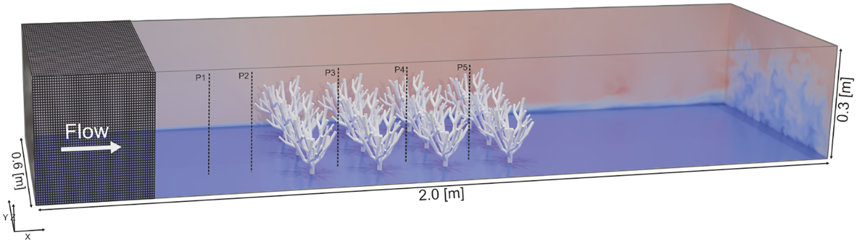
Figure 1. The numerical model is shown in three dimensions, indicating the domain size, the positioning of the cold-water coral colonies, and the mesh (in dark grey). For visual representation of the flow field in this model setup, the blue to red color gradient represents the flow velocity magnitude (U), with blue indicating lower velocities and red indicating higher velocities. P1-P5 indicate the locations of velocity and sediment concentration measurement profiles at y=0.2, along the domain’s length.

The flow in the numerical model was designed to be unidirectional, entering from the left (upstream) and exiting to the right (downstream). Therefore, the following boundary conditions were set: a fixed velocity inlet on the left face (X-min) and a velocity inlet/outlet on the right face (X-max). The front (Y-min) and back (Y-max) walls of the domain were set with zeroGradient conditions for velocity to simulate frictionless symmetry planes. The bottom (Z-min) and coral structures were set with no-slip conditions to simulate seabed and coral interactions with the flow. In contrast, the top wall (Z-max) was assigned a slip condition, enforcing zero normal velocity (preventing mass flux through this boundary) and zero shear stress, approximating a frictionless rigid lid. The inlet flow was set with no background turbulent perturbations to focus on coral-induced turbulence, with a velocity of U = 0.1 m/s, which is within the range of near-bed currents observed in cold-water coral habitats (Mienis et al., 2007). For sediment transport modeling, a sediment influx at the inlet with a concentration of 0.1 g/l was introduced, selected for consistency with validated multiphase sediment simulations in Le Minor et al. (2019), which validated the driftFluxFOAM solver against settling experiments for accurate representation of suspension and deposition processes. The minimum sediment concentration of 0.1 g/L is a direct result of the constant sediment inlet condition, which is maintained throughout the domain due to the unidirectional flow. This flow, governed by the transport equation, combined with no-slip conditions at the walls and coral structures and a slip condition at the top, prevents any reduction below this value. The introduced sediment corresponds to a medium silt grain size (17 μm particle size) and a density of 2650 kg/m³, as documented by Byun and Wang (2005). This specific type of sediment was selected due to its relevance to the environmental conditions typical for cold-water coral reefs (e.g., Wang et al., 2021).

Fluid properties were selected with a kinematic viscosity (ν) of 1e-6 m²/s and a density (ρ) of 1000 kg/m³, consistent with prior laboratory flume experiments used for model validation (Bartzke et al., 2021). These values closely approximate seawater properties at typical cold-water coral temperatures (4–12 °C), where density is approximately 1025–1027 kg/m³ and kinematic viscosity is 1.3–1.5e-6 m²/s (Sharqawy et al., 2010). The small differences have negligible impact on the simulated hydrodynamic and sediment dynamics, as the flow regime remains comparable. Each simulation represents 30 seconds of real-time with time steps of a maximum of 0.0025 seconds. The Courant–Friedrichs–Lewy (CFL) number was constantly monitored to stay below 0.1, ensuring the stability of the numerical simulations. The CFL, a measure for numerical stability and time-stepping, is defined as CFL= $\text{u}\Delta \text{t}/\Delta \text{x}$ where $u$ refers to the velocity, $\text{t }$ to the time step, and $\Delta \text{x}$ to the streamwise cell distance. A CFL below 1 is the commonly accepted criterion for such numerical stability (Courant et al., 1928; Ferziger and Perić, 2002). In addition, it needs to be noted that in previous research, this model’s accuracy was benchmarked against laboratory flume experiments (Bartzke et al., 2021). In addition, the sediment concentration dynamics computed by the present solver have been rigorously benchmarked and validated in prior works by Le Minor et al. (2019).

2.3 Post-processing of simulation data

All post-processing and visualization tasks were conducted using Matlab and paraFoam, a version of ParaView specifically adapted for OpenFOAM. Data from the simulation at t=30 seconds was used for analysis to ensure the flow had fully stabilized around the centrally located corals in the computational domain, providing a coherent and accurate representation of hydrodynamic behavior. To enhance visualization and interpretation, slices were taken along the Y and Z axes within the computational domain. These slices captured both instantaneous and mean flow conditions, as well as sediment distribution patterns, offering detailed insights into the interplay between flow and sediment dynamics near the coral structures. The mean flow refers to the time-averaged velocity field (UMean in OpenFOAM nomenclature), which was computed by averaging the instantaneous velocity fields over time. Vertical measurement profiles, indicated by the vertical dashed lines in Figure 1, were generated from the numerical model at five strategically selected spots. These profiles, all placed at Y = 0.2 m, included a position at X = 0.5 m, representing the undisturbed upstream flow, and positions at X = 0.575 m, X = 0.745 m, X = 0.915 m, and X = 1.085 m within the corals for comparative analysis. To provide a comprehensive view of the flow behavior, the mean velocity components were plotted, with a focus on the downstream velocity component (Ux). Each profile consisted of 2000 data points. Sediment concentration profiles were also generated at the same locations to thoroughly analyze sediment dynamics relative to coral placement.

To understand the resistance exerted by the coral structures on the flow, taking into account both the physical characteristics of the corals and the flow dynamics, we calculated the drag forces on all the coral colonies. This approach also served as a validation step, enabling comparisons with findings from previous studies. The pressure values facing against the flow direction were analyzed, highlighting zones of high and low normal pressure. These pressures were integrated over the coral colony surfaces using ParaView’s ‘Extract Surface Normals’ and ‘Integrate Variables’ filters. The area of the coral colony surfaces, provided as part of the field data in ParaView, was used in conjunction with the integrated pressure data to compute the drag force (Fd). The drag coefficient (Cd) was then calculated using this force data, fluid density (ρ), and velocity (U). Additionally, the Turbulent Kinetic Energy (TKE) distribution was computed using the Reynolds stresses derived from the OpenFOAM simulation, calculating the TKE magnitude as:

$TKE=0.5 (u^{\text{'}2}+v^{\text{'}2}+w^{\text{'}2})$ where $u^{\text{'}2}$, $v^{\text{'}2}$, and $w^{\text{'}2}$ are the diagonal components of the Reynolds stress tensor representing the variance of velocity fluctuations in the X, Y, and Z directions, respectively (Pope, 2000). The TKE distribution was then visualized in ParaView by applying a calculator filter to the entire Reynolds stresses field, enabling the spatial analysis of turbulence intensity across the domain.

3 Results

3.1 Flow dynamics around the cold-water corals

The instantaneous flow velocity at t=30 s and the time-averaged flow velocity around the corals are illustrated in Figure 2. The figures display slices oriented in both the Y-normal and Z-normal directions. The locations of the Z-normal slices were chosen close to the bottom of the domain, near the stems of the cold-water corals at Z = 0.005 m, as well as within the branches, which were processed at Z = 0.1 m. As a result, all slices reveal patterns in the velocity field values throughout the domain and provide representative insight into the flow dynamics, particularly in the vicinity of the coral structures.

Figure 2

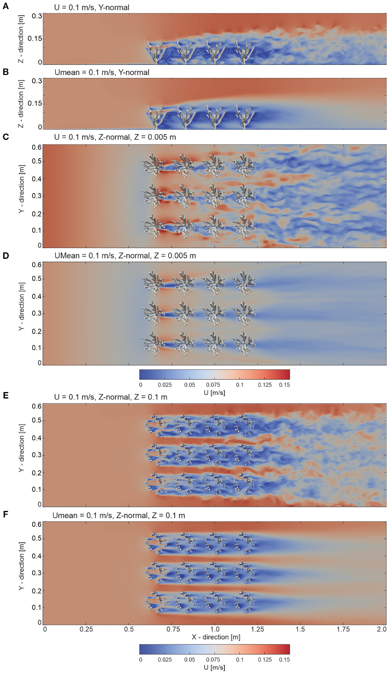
Figure 2. Overview of the instantaneous velocity field (U) at t = 30 s and the mean streamwise velocity field (time-averaged over t=0–30 s,.Umean) from the numerical model with an inlet boundary condition velocity of 0.1 m/s. Slices are presented as follows: (A) instantaneous and (B) mean velocity fields in the y-normal plane at y = 0.3 m; (C) instantaneous and (D) mean velocity fields in the z-normal plane near the bed at z = 0.005 m; and (E) instantaneous and (F) mean velocity fields in the z-normal plane within the coral canopy at z = 0.1 m.

The flow interaction with the cold-water coral structures showed a distinct pattern. From the beginning of the domain up to the first encounter with the coral structures (X = 0 to X = 0.55 m), the flow predominantly exhibited a nearly uniform character. Nonetheless, in the region before the flow encountered the cold-water corals, ranging approximately from X = 0.50 to X = 0.55 m, a noticeable decrease in flow speeds was observed. This indicated the onset of flow reduction due to the interaction with the coral structures. In the region where the flow directly interacts with the complex cold-water coral structures (X = 0.55 to X = 1.25 m), significant variations in flow speed were observed. Above the corals (X = 0.55 to X = 2.0 m and Z = 0.15 to Z = 0.3 m), the flow remained relatively unperturbed, but slightly enhanced mixing occurred at the coral–freestream boundary. Within the spaces between the corals, flow speeds decreased progressively downstream. As the flow progressed downstream of the corals (from X = 1.25 to X = 2.0 m), varying velocities were observed, a phenomenon which can be attributed to flow separation caused by the coral branches (Figure 2).

Observing the velocity field near the bed (Z = 0.005 m) and within the coral branches (Z = 0.1 m) within the coral-influenced region (X = 0.55 to X = 1.25 m) highlights notable differences. Near the bed, the flow velocity distribution showed a relatively structured pattern, with low velocities of approximately 0.02 m/s to 0.04 m/s in dominating the leeside of the coral stems. In the inter-coral gaps (i.e. the continuous long coral-free areas parallel to the flow direction), higher velocities of around 0.06 m/s to 0.09 m/s were observed, with distinct low-velocity zones behind the stems. In contrast, within the coral branches (Z = 0.1 m, X = 0.55 to X = 1.25 m), the flow field exhibited high variability due to interactions with the complex coral structure. The velocity magnitudes ranged from 0.03 m/s in low-velocity zones to 0.13 m/s in high-velocity patches, reflecting increased turbulence and disrupted flow patterns. Specifically, high velocities of 0.1 m/s to 0.13 m/s were observed in the inter-coral gaps, while low velocities of 0.03 m/s to 0.06 m/s occurred in the wake of the branches, creating highly dynamic zones of flow redistribution near the individual coral branches. This complexity underscores the cumulative effect of coral structures in obstructing and redistributing the flow as it moves downstream. The time-averaged velocity distribution, illustrated in Figure 2, showcased a similar pattern, emphasizing the differences in flow behavior between the bed and the coral canopy regions.

Consequently, the results shown in Figures 2 allow for categorizing the findings into three key regions: the undisturbed region (X = 0 to X = 0.55 m), the coral-influenced region (X = 0.55 to X = 1.25 m), and the wake region (X = 1.25 to X = 2.0 m). In the undisturbed region (from X = 0 to X = 0.55 m), the flow largely maintained a consistent velocity of around 0.1 m/s, with only minor fluctuations, indicating a uniform and stable flow unaffected by external disturbances. However, a slight flow reduction directly in front of the corals was observed. Upon entering the coral-influenced region (from X = 0.55 to X = 1.25 m and Z = 0 to Z = 0.1 m), this uniformity was disrupted. The coral branches significantly altered the flow, created localized high-velocity regions of up to 0.13 m/s near their surfaces, while intensified turbulence in the surrounding flow. Within the coral canopy, this region became a zone of complex flow interactions, characterized by eddies, vortex formations, and swirling motions. The branches disrupted the uniform flow and contributed to the formation of alternating zones of acceleration and deceleration, driven by flow obstruction and vortex shedding around the branches. These dynamics highlight the role of the branches in amplifying flow disturbance and promoting mixing within the coral-influenced region, contrasting with the relatively structured flow observed at the bed level. Yet, just above the corals, an undisturbed flow persisted, reflecting undisturbed flow patterns also observed in the undisturbed region, although slightly enhanced mixing occurred at the canopy–freestream boundary. In the wake region (from X = 1.25 to X = 2.0), the flow exhibited subtle contrasts, with velocities fluctuating between 0.07 m/s and 0.11 m/s, reflecting the ongoing influence of the corals on the flow.

3.2 Fluid flow profiles

The hydrodynamic profiles presented in Figure 3 offer a detailed insight into fluid behavior across the undisturbed region and the coral-influenced region, spanning from X = 0.5 m to X = 1.085 m, at Y = 0.2 m. In P1 (Profile 1 at X = 0.5 m), serving as a reference for undisturbed flow, and P2 (Profile 2 at X = 0.575 m), positioned closely to capture transitional velocity changes, both located in the undisturbed region, the profiles revealed a very similar pattern, with P2 showing slightly decreased velocities. They showed a distinctive logarithmic trend with an almost linear gradient in velocities from the top of the domain (Z = 0.3 m) down to near the bottom (Z = 0.025 m). As the profiles approached the bottom of the domain, a noticeable transition occurred, with the flow gradient smoothly converging towards zero velocity. Moving into the coral-influenced region, P3 (Profile 3 at X = 0.745 m), P4 (Profile 4 at X = 0.915 m), and P5 (Profile 5 at X = 1.085 m), changes in the velocity gradients were noticeable. In these profiles, the upper sections maintained linearity—specifically, up to Z = 0.15 m for P3, Z = 0.2 m for P4, and Z = 0.225 m for P5, although a slightly enhanced velocity increase occurred at these canopy–freestream boundaries. Below these heights, the linear gradients changed to a gentle, irregular pattern in flow velocities, highlighting the interplay between fluid dynamics and the coral structures. Below these heights, the linear gradients changed to a gentle, undulated pattern in flow velocities, with peaks reaching up to approximately 0.09 m/s, reflecting the dynamic interaction between the flow and the coral structures.

Figure 3

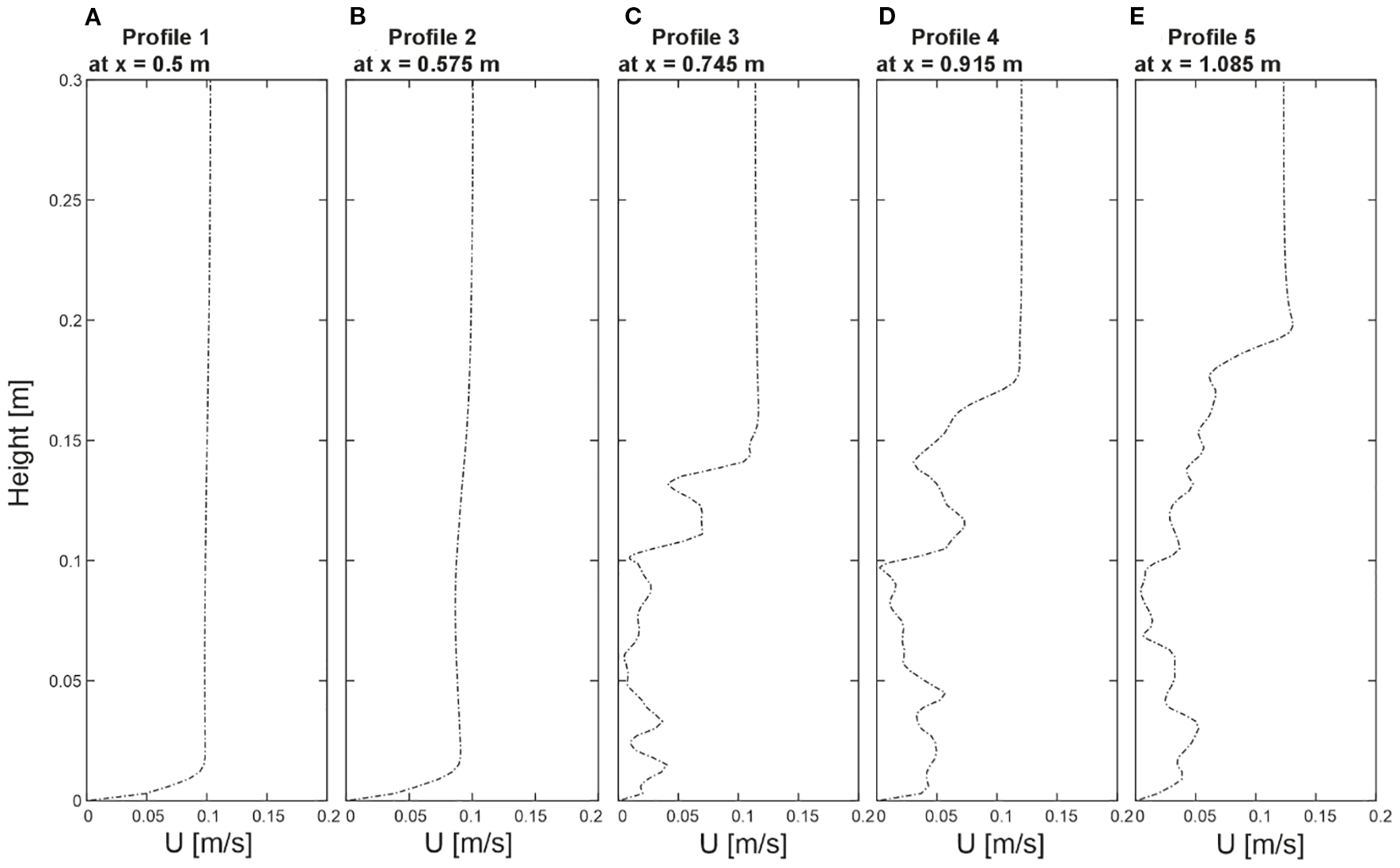
Figure 3. (A–E) Velocity profiles extracted from five positions of the numerical model. The distinct profile locations are indicated in Figure 1. Profiles are taken from Profile1 at x=0.5 m, Profile2 at x=0.575 m, Profile3 at x=0.745 m, Profile4 at x=0.915 m, and Profile5 at x=1.085 m at y=0.2 m, illustrating the flow distribution over height (Z).

3.3 Drag forces

The velocity and pressure values were used to compute the drag forces exerted on the cold-water corals in the tested flow scenario. In the tested flow velocity scenario, the drag force was calculated to be 0.30 N/m², and the computed drag coefficient (Cd) was determined to be 0.12. This result aligns with the expected relationship between flow speed and drag force, where, for example, decreases in flow speed lead to corresponding reductions in drag force.

3.4 Turbulent kinetic energy distribution and 3D turbulent structures

To show the energy distribution within the cold-water coral canopy, the turbulent kinetic energy (TKE) distribution processed from the 30-second time step is presented in Figure 4. In the upstream region of the model domain (X = 0.0 m to X = 0.55 m, Figure 4A), no turbulent kinetic energy was evident. This was related to the inflow boundary condition of the model, where no background turbulent perturbations were specified, which allowed us to focus solely on the turbulence generated by the corals themselves. Within the coral-influenced zone (X = 0.55 m to X = 1.25 m), a subsequent increase in TKE values was observed as the flow interacted with the corals. A concentrated increase in TKE values was particularly evident in the leeside of the corals close to the bottom of the domain (Z = 0.005 m), indicated by values to 0.0006 m²/s². However, within the inter-coral gaps (Figure 4B) the TKE values were lower with values in the range of 0.0001 to 0.0002 m²/s². Further upward (Z = 0.10 m), within branches of the corals (Figure 4C), a broader TKE value distribution was evident, spreading laterally and downstream. TKE values appeared to be enhanced directly in the lee side of the branches. TKE values appeared to originate directly in the lee side of the branches. Here, interaction effects between neighboring coral structures were also evident, contributing to a complex turbulent field with values ranging towards 0.0006 m²/s², trailing downstream and increasing towards the end of the domain (X = 1.55 to 2.00 m).

Figure 4

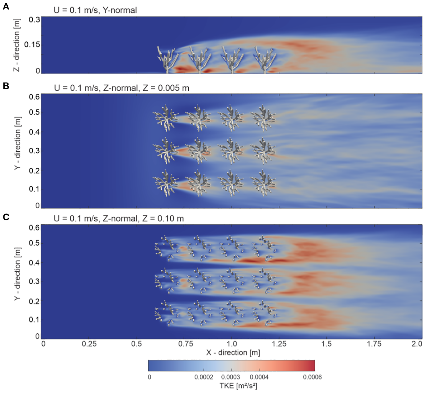
Figure 4. Visualization of turbulent kinetic energy (TKE) distribution within a cold-water coral canopy with an inlet boundary condition velocity of 0.1 m/s. The TKE is shown for three cross-sections: (A) Y-normal plane at Z = 0.33 m, (B) Z-normal plane at Z = 0.005 m, and (C) Z-normal plane at Z = 0.10 m.

3.5 Sediment dynamics around the cold-water corals

The instantaneous sediment concentration at the 30-second time step, along with the time-averaged sediment concentration field surrounding the coral structures, are illustrated in Figure 5. Slices oriented in both Y-normal and Z-normal directions, analogous to the fluid velocity fields, provide a representative view of the sediment concentration patterns across the domain. High sediment concentrations typically occurred in regions where turbulent kinetic energy is low. Conversely, areas with higher turbulence tended to exhibit lower concentrations due to increased mixing. This is consistent with the drift-flux transport formulation used in the numerical solver, where sediment accumulation results from the local balance between settling velocity and turbulence-driven mixing, as the settling velocity allows particles to deposit in low-turbulence zones while mixing disperses them in high-turbulence areas.

Figure 5

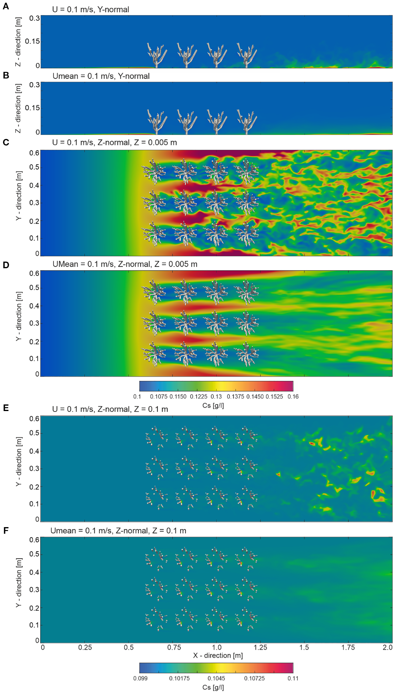
Figure 5. Overview of the instantaneous and mean sediment concentration fields from the numerical model at t=30 s with an inlet boundary condition velocity of 0.1 m/s. Slices are presented as follows: (A) instantaneous and (B) mean sediment concentration fields in the y-normal plane at y = 0.3 m; (C) instantaneous and (D) mean sediment concentration fields in the z-normal plane near the bed at z = 0.005 m; and (E) instantaneous and (F) mean sediment concentration fields in the z-normal plane within the coral branches at z = 0.1 m.

The slices shown in Figure 5, indicate that sediment distribution in the undisturbed region upstream of the cold-water corals (from X = 0 to X = 0.55 m) exhibited a uniform pattern, averaging around 0.1 g/L. The uniformity in sediment distribution suggests that the flow remained steady and relatively undisturbed before encountering the coral structures downstream. However, an increase in sediment concentration to approximately 0.13 g/L was observable close to the bed at Z = 0.005 m, from X = 0.50 to X = 0.55 m, towards the onset of the coral canopy, corresponding to the reduction in flow velocity in this region.

As the flow moved into the coral-influenced zone (X = 0.55 to X = 1.25 m), a noticeable change in sediment distribution occurred. In contrast to the uniformity observed upstream, among the corals varied sediment concentration patterns can be seen. Concentrations in the coral-influenced region varied between 0.099 and 0.16 g/L, reflecting complex sediment–structure interactions. Near the bed at Z = 0.005 m, local maxima up to 0.16 g/L were found in inter-coral gaps, where sediment concentrations increased. In contrast, lower concentrations, averaging around 0.1 g/L, occurred in the lee of individual coral stems. Within the branches at Z = 0.1 m, sediment accumulation was concentrated in the low-energy zones between coral branches, while vertically, the sediment concentration above the corals (> 0.1 m) remained relatively homogeneous at approximately 0.1 g/l. This uniformity indicated that coral-induced disturbances had a localized effect and did not significantly alter sediment concentrations in the overlying water layers. In the wake region, ranging from X = 1.25 to X = 2.0 m, the sediment distribution became increasingly complex, with concentrations fluctuating between 0.1 g/L and 0.115 g/L. Higher concentrations, reaching up to 0.115 g/L, were observed near the bed at Z = 0.005 m in depositional zones between eddies, though these values are lower than the peak concentrations in the coral-influenced zone. Conversely, concentrations remained closer to 0.1 g/L in the upper layers (Z > 0.1 m), reflecting the persistent influence of coral-fluid interactions. This pattern resulted from turbulent mixing, eddies, and vortices shed by the corals, which drive localized sediment resuspension and deposition in the wake.

3.6 Sediment concentration profiles

Building on the elevated sediment distributions in Section 3.5, this section focuses on quantitative profiles at the bed level to illustrate the near-bottom accumulation. Sediment concentration profiles revealed a complex interaction between sediment dynamics and cold-water coral structures. As illustrated in Figure 6, the profiles between X = 0.5 m and X = 1.085 m encompassed both undisturbed and coral-influenced regions at Y = 0.15 m. Note that these profiles showed concentrations at the bed (Z = 0 m), where sediment accumulation was highest, compared to the slightly elevated slices (Z = 0.005 m and Z = 0.1 m) in Figure 5. In the undisturbed region, Profile 1 (P1) at X = 0.5 recorded a sediment concentration of 0.145 g/l at Z = 0 m, while Profile 2 (P2) at X = 0.575 m showed a slightly higher concentration of 0.148 g/l. This consistent pattern in areas not yet directly influenced by coral structures reflected both the steady sediment supply from the inlet boundary and the gradual reduction in flow velocity upstream of the coral canopy, which favored early sediment settling. As the flow interacted with the coral structures, Profiles 3 (P3) at X = 0.745 m, 4 (P4) at X = 0.915 m, and 5 (P5) at X = 1.085 m revealed a slight decline in sediment concentration. For example, in Profile 3, the concentration was approximately 0.114 g/L near the bottom, decreasing with height. Profile 4 showed a similar pattern, starting at 0.115 g/L at the bottom, while Profile 5 had a slightly higher 0.116 g/L, both decreasing upward. These profiles suggest that cold-water corals significantly influence sediment dynamics, particularly by promoting sediment accumulation near the bottom, but lower compared to P1 and P2. However, as the flow progressed downstream, the overall sediment distribution began to stabilize. The consistent pattern observed across Profiles 3, 4, and 5 indicated that the coral structures exert a persistent influence on sediment transport.

Figure 6

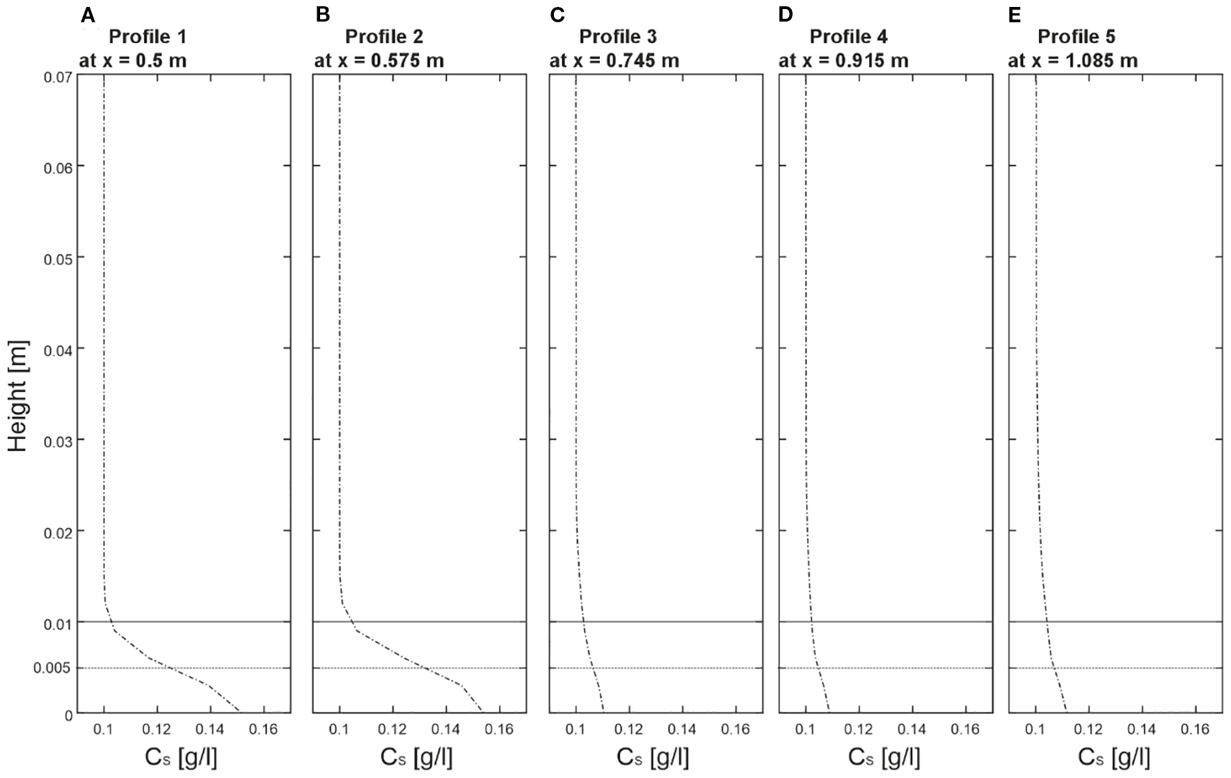
Figure 6. (A–E) Overview of the sediment concentration profiles extracted from five positions of the numerical model. Profiles are taken from Profile 1 at x=0.5 m, Profile 2 at x=0.575 m, Profile 3 at x=0.915 m, and Profile 5 at x=1.085 m at y=0.2, illustrating the sediment concentration value distribution over height.

4 Discussion

In this study we use a three-dimensional Computational Fluid Dynamics (CFD) model to analyze the interactions between fluid flow, turbulent structures, and sediment dynamics in a cold-water coral colony. The model’s hydrodynamic and sedimentological findings are interpreted to understand deposition processes potentially driving the early stages of mound aggradation. Our findings demonstrate that cold-water corals significantly alter hydrodynamic patterns and sediment dynamics, promoting sediment deposition. Distinct sediment distribution patterns were observed, with sediment preferentially deposited in inter-coral gaps near the bed where mean flow delivers particles and reduced turbulence allows their settling. In contrast, within the branches, low mean velocities combined with high turbulent kinetic energy maintain particles in suspension, resulting in more heterogeneous concentrations. The inter-coral gaps provide “spaces” where sediment can settle, playing a dominant role in shaping the observed patterns and establishing them as the primary sites of accumulation. The interplay between high TKE-driven ongoing suspension on the lee side stems, lateral transport toward the inter-coral gaps, and lower turbulence facilitating deposition in inter-coral gaps underlines the complex sediment-trapping mechanism induced by the corals. These findings highlight the capacity of coral colonies to shape sediment dynamics through their structural influence on hydrodynamics, providing insights into potential contributions to the sediment budget and the initiation of coral mound formation, particularly near the bed where accumulation is consistent.

4.1 Fluid dynamics around the cold-water corals

The use of the three-dimensional numerical model provides detailed insights into how cold-water corals influence hydrodynamics. As part of model validation, the drag coefficient (Cd) is a crucial parameter for quantifying the resistance cold-water corals impose on flow; our findings reveal a Cd value of 0.12, which aligns closely with established literature values. For example, Samuel and Monismith (2013) reported a Cd value relevant for coral colonies, potentially applicable to cold-water corals, under flow velocities between 0.02 m/s and 0.26 m/s. Similarly, Lentz et al. (2017) found a Cd range of 0.005–0.2 for coral reefs, with values around 0.12 plausible for deeper waters under flow velocities ranging from 0.05 m/s to 0.5 m/s. Comparable findings are also reported in studies of coral hydrodynamics, such as by Rosman and Hench (2011), who documented Cd values in the range of 0.01–0.8 influenced by canopy geometry, thus supporting the plausibility of a Cd of 0.12. This close agreement with previous studies confirms the validity of our model in simulating the hydrodynamic interactions of cold-water corals.

Previous research focusing on the flow dynamics around a single coral colony observed deceleration in flow due to the presence of the coral (Bartzke et al., 2021). This observation is in line with the findings of the current study, which expanded the analysis to an array of 12 coral colonies arranged in a 3 by 4 grid under flow velocities typical for cold-water coral habitats (Roberts et al., 2009). The results of the numerical model indicate that the corals exert a pronounced effect on the flow, with the changes caused by one cold-water coral affecting the flow conditions experienced by adjacent cold-water corals. This effect varies vertically: near the bed, flow deceleration is pronounced at the leeside, behind stems, creating structured low-velocity zones accompanied by high turbulent kinetic energy, while within the branches, the flow exhibits greater variability and disruption due to the complex coral structure generating elevated turbulent kinetic energy. As a result, the spatial variations in flow reduction—marked by pronounced deceleration near the bed and greater variability within the branches—lead to emergent flow patterns influenced by the arrangement and orientation of the coral colonies. These complex flow patterns around multiple corals mirror observations from research on tropical coral flow dynamics, such as those by Hench and Rosman (2013). They observed that the flow downstream from one coral colony can be significantly altered by the presence of another colony, highlighting the intricate hydrodynamic interactions between colonies. These findings also suggest that the orientation of individual coral branches relative to the flow direction can directly influence the flow’s direction.

The model results demonstrate that cold-water coral structures profoundly influence the distribution of turbulent kinetic energy (TKE) within their vicinity, playing a critical role in shaping sediment mobilization, transport, and deposition patterns across the coral canopy. Near the bed, particularly in the wake zones behind coral stems, high TKE levels were observed. This turbulence promotes the dynamic suspension of sediments from the immediate vicinity of the stems, mobilizing particles that are then transported laterally into the inter-coral gaps, where turbulence is notably lower. These low-energy zones serve as depositional areas, facilitating the accumulation of sediments, as further explored in Section 4.2. In contrast, within the coral branches, the TKE distribution is more diffuse, stemming from direct interactions between the flow and the branch structures. The localized nature of this turbulence creates protected zones immediately behind the branches, offering ideal conditions for the deposition of fine particles with minimal lateral redistribution into the inter-coral gaps. Consequently, the model reveals two distinct TKE-driven processes within the coral canopy. High TKE near the bed promotes dynamic suspension and lateral transport, enriching the inter-coral gaps as low-energy zones trap mobilized sediments. These results align with prior studies, such as Roberts et al. (2009) and Mienis et al. (2012), which highlight how cold-water corals act as obstacles, altering hydrodynamics and sediment transport, for instance by generating upwelling and downwelling that enhance nutrient delivery and sediment resuspension in ways consistent with our TKE patterns. Parallels also emerge with Wheeler et al. (2007), who noted the role of turbulent flow in redistributing sediments around coral mounds.

The results of the numerical model also demonstrate how cold-water corals modify flow patterns in their vicinity. As the flow encounters the coral structures, a marked shift occurs, transitioning from uniform to an altered flow pattern characterized by localized deceleration and acceleration zones around the corals, as evidenced by changes in flow velocity and elevated TKE values. This modification in flow, particularly intensified by interactions among multiple corals, enhances food supply by increasing both the delivery and retention of suspended particles near the coral polyps, thereby supporting their health, growth, and reproductive capacity (Frederiksen et al., 1992; Davies et al., 2009). Furthermore, the emergence of a distinct zone of stable velocities above the canopy may suggest a vertical gradient in food distribution within the coral habitat. This gradient could indicate the presence of vertical ecological niches within the coral ecosystem, consistent with observations of vertical flow structuring and food supply mechanisms in cold-water coral reefs (Thiem et al., 2006; Mienis et al., 2007). Nonetheless, the model assumes a steady, uniform, and undisturbed inflow at the inlet, emphasizing the changes in velocity induced by the coral structures themselves. In natural settings, however, the approaching flow likely exhibits pre-existing velocity variations, which could further shape the flow dynamics created by the corals.

4.2 Sediment dynamics around the cold-water corals

The model results indicate that cold-water corals significantly influence sediment dynamics in their vicinity by causing flow deceleration through physical obstruction, as supported by Mienis et al. (2007). The constant sediment introduction at the inlet ensures a steady upstream supply, contributing to additional sediment loading towards the canopy. High turbulent kinetic energy near the bed mobilizes sediment particles in the downstream of individual coral stems. These sediments are then redistributed and accumulate preferentially in the inter-coral gaps, where reduced turbulence facilitates deposition despite higher flow velocities, leading to elevated concentrations near the bed compared to the leeside zones. In contrast, within the branches, sediment deposition is more variable due to localized flow perturbations, with accumulation primarily occurring in small, sheltered zones behind the branches, while the leeside of individual branches shows lower concentrations due to turbulence-driven resuspension. Above the coral canopy, sediment concentrations remain relatively homogeneous, indicating that coral-induced disturbances are largely confined to the lower regions of the domain. This trapping and accumulation of sediment, particularly in inter-coral gaps, is critical for understanding mound formation processes and supporting the growth of cold-water coral communities by providing an elevated habitat, as postulated by Roberts et al. (2006) and Dorschel et al. (2007). Comparing these findings with previous studies, such as Bartzke et al. (2021), parallels are evident in how cold-water corals act as obstacles influencing hydrodynamics and, consequently, sediment transport, providing a foundation for further exploring their role in mound aggradation.

4.3 Implications for mound formation

The numerical model provides essential insights into the hydrodynamic and sedimentary conditions around cold-water coral colonies. We observed that sediment deposition patterns near cold-water corals are influenced by varying hydrodynamic conditions. In regions of reduced turbulence, such as the inter-coral gaps and sheltered zones behind branches, sediment trapping is enhanced. Assuming a consistent sediment supply and stable environmental conditions (e.g., appropriate temperature, nutrient availability, and limited disturbance by strong currents), these micro-scale trapping processes could contribute to the early stages of mound aggradation, particularly for fine sediments as modeled. The extent of sediment accumulation, however, depends strongly on granulometry. Coarser particles may settle more readily while finer ones remain longer in suspension, and terrigenous fractions—which often constitute a significant proportion of mound sediments—are likely to play a key role in long-term stabilization and mound buildup (Pirlet et al., 2011). Thus, regions with naturally faster water flows might experience varying degrees of sediment accumulation based on the specific sediment characteristics present, which could potentially affect the rate of mound growth. Beyond the micro-scale, recent work by van der Kaaden et al. (2021) demonstrated that the structural presence of coral mounds modulates local hydrodynamics at larger scales, including enhanced turbulent energy dissipation and the trapping of internal tides, thereby increasing particle flux toward the coral framework. While their study focused on mound-scale feedbacks, our findings illustrate a complementary process at the colony scale: coral structures act as ecosystem engineers by creating sheltered zones, reducing local turbulence, and facilitating sediment accumulation. Together, these multi-scale processes highlight the potential mechanistic pathways from small-scale trapping to mound initiation and vertical growth. While our numerical model cannot directly capture geological timescales, the results provide mechanistic insights that may inform hypotheses on early mound initiation. Therefore, continuous sediment deposition in low-flow areas could lead to substantial coral mound development over several millennia. This could particularly be the case in areas along the Atlantic Ocean’s continental margins, known for coral mounds comprising skeletal fragments and hemipelagic sediments. However, these are speculative assertions and warrant further observational or modeling studies for validation. Nonetheless, the results underscore how coral–flow–sediment interactions provide a foundation for mound formation along Atlantic margins, where sediment supply and hydrodynamic forcing drive the development of carbonate mounds composed largely of hemipelagic sediments and skeletal fragments (Wheeler et al., 2007; Wang et al., 2021).

4.4 Limitations and future steps

The present study has provided insights into the interactions between cold-water corals and their surrounding hydro and sediment dynamics. While the model employed focused on a specific coral configuration, it highlights the necessity for broader research encompassing various cold-water coral reefs. Expanding the scope of investigation would significantly deepen our understanding of coral mound formation on larger spatial scales. One promising direction for future research is the integration of detailed 3D coral scans into numerical models, allowing for a more comprehensive analysis of coral behavior under diverse flow and sedimentation conditions. However, this advanced methodology faces significant computational challenges, requiring high-performance computing clusters beyond the scope of standard computational resources. Additionally, investigating the collective effects of large-scale reefs on hydrodynamic and sedimentary processes, especially the role of sediment deposition in mound formation, remains a critical area of study. The present model assumed zero background turbulence at the inlet, thereby isolating the effects of coral-induced turbulence. In natural settings, pre-existing (inlet) turbulence may amplify or modify the observed patterns. Despite these challenges, the present research lays a solid foundation, paving the way for more extensive future studies to further unravel the complex dynamics of cold-water corals within marine ecosystems.

5 Conclusion

A three-dimensional Computational Fluid Dynamics (CFD) model was used to examine the interactions between fluid flow, turbulent structures, and sediment dynamics in the vicinity of a cold-water coral colony. The analysis employed the simulation of a setup comprising 12 coral colonies arranged in a 3x4 grid, subjected to flow velocities representative of typical cold-water coral habitats. The model assessed the influence of coral geometry on hydrodynamic patterns, as well as on the mobilization, transport, and deposition of sediments, with a constant inlet sediment concentration established as the baseline condition. The results show that cold-water corals exert a significant influence on both flow and sediment dynamics, facilitating spatially heterogeneous sediment transport and deposition patterns. Several key finding emerge: (1) the inlet concentration is modulated by coral-induced turbulence, resulting in spatially variable sediment dynamics; (2) dynamic sediment suspension is primarily associated with elevated turbulent kinetic energy (TKE) and moderate flow velocities, suggesting a consistent turbulence-driven sediment transport process; (3) deposition is markedly enhanced near the seabed and within inter-coral gaps, where reduced velocities and increased concentrations indicate sediment accumulation driven by flow retardation; and (4) intensified TKE between coral structures redistributes sediment, underscoring the pivotal role of coral geometry in modulating local hydrodynamic conditions. The geometry of the coral colonies—particularly their spacing, height, and branching complexity—creates localized funneling and open zones, which in turn determine where sediments are mobilized, retained, or redeposited. These findings underscore the profound influence of coral structures on sediment budgets and the initiation of mound formation, establishing a robust framework for advancing future investigations into the ecological dynamics of cold-water coral ecosystems.

Data availability statement

The original contributions presented in the study are included in the article. Further inquiries can be directed to the corresponding author.

Author contributions

GB: Writing – review & editing, Writing – original draft. DH: Writing – review & editing, Writing – original draft. KH: Writing – review & editing, Writing – original draft.

Funding

The author(s) declare financial support was received for the research and/or publication of this article. This work has been funded through funded through the Cluster of Excellence “The Ocean Floor – Earth’s Uncharted Interface“. G. B. was supported by the BMBF DAM MultiMAREX project (03F0952E).

Acknowledgments

We gratefully acknowledge the constructive help by Emil Rietschel.

Conflict of interest

The authors declare that the research was conducted in the absence of any commercial or financial relationships that could be construed as a potential conflict of interest.

Generative AI statement

The author(s) declare that Generative AI was used in the creation of this manuscript. Generative AI tools were used to support language editing and structural improvements of the manuscript. All scientific content, data interpretation, and conclusions were entirely generated by the authors.

Any alternative text (alt text) provided alongside figures in this article has been generated by Frontiers with the support of artificial intelligence and reasonable efforts have been made to ensure accuracy, including review by the authors wherever possible. If you identify any issues, please contact us.

Publisher’s note

All claims expressed in this article are solely those of the authors and do not necessarily represent those of their affiliated organizations, or those of the publisher, the editors and the reviewers. Any product that may be evaluated in this article, or claim that may be made by its manufacturer, is not guaranteed or endorsed by the publisher.

References

Bartzke G., Siemann L., Büssing R., Nardone P., Katinka K., Hebbeln D., et al. (2021). Investigating the prevailing hydrodynamics around a cold-water coral colony using a physical and a numerical approach. Front. Mar. Sci. 8. doi: 10.3389/fmars.2021.663304

Crossref Full Text | Google Scholar

Byun D.-S. and Wang X. H. (2005). The effect of sediment stratification on tidal dynamics and sediment transport patterns. J. Geophys. Res. 110, C09025. doi: 10.1029/2004JC002459

Crossref Full Text | Google Scholar

Corbera G., Lo Iacono C., Simarro G., Lo Iacono C., Lo Iacono C., Standish C. D., et al. (2022). Local-scale feedbacks influencing cold-water coral growth and subsequent reef formation. Sci. Rep. 12, 20389. doi: 10.1038/s41598-022-24711-7

PubMed Abstract | Crossref Full Text | Google Scholar

Courant R., Friedrichs K., and Lewy H. (1928). On the partial difference equations of mathematical physics. Math. Ann. 100, 32–74. doi: 10.1007/BF01448839

Crossref Full Text | Google Scholar

Davies A. J., Duineveld G. C. A., Lavaleye M. S. S., Bergman M. J. N., and Van Haren H. (2009). Downwelling and deep-water bottom currents as food supply mechanisms to the cold-water coral Lophelia pertusa (Scleractinia) at the Mingulay Reef complex. Limnol. Oceanogr. 54, 620–629. doi: 10.4319/lo.2009.54.2.0620

Crossref Full Text | Google Scholar

Dorschel B., Hebbeln D., Rüggeberg A., Wienberg C., and Freiwald A. (2007). Carbonate budget of a cold-water coral carbonate mound: Propeller Mound, Porcupine Seabight. Int. J. Earth Sci. 96, 73–83. doi: 10.1007/s00531-005-0493-0

Crossref Full Text | Google Scholar

Drikakis D. and Rider W. J. (2005). High-resolution methods for incompressible and low-speed flows (Berlin, Heidelberg: Springer).

Google Scholar

Ferziger J. H. and Perić M. (2002). Computational methods for fluid dynamics. 3rd ed (Berlin, Heidelberg: Springer).

Google Scholar

Frederiksen R., Jensen A., and Westerberg H. (1992). The distribution of the scleractinian coral Lophelia pertusa around the Faroe Islands and the relation to internal tidal mixing. Sarsia 77, 157–171. doi: 10.1080/00364827.1992.10413502

Crossref Full Text | Google Scholar

Germano M., Piomelli U., Moin P., and Cabot W. H. (1991). A dynamic subgrid-scale eddy viscosity model. Phys. Fluids A 3, 1760–1765. doi: 10.1063/1.857955

Crossref Full Text | Google Scholar

Godunov S. K. and Bohachevsky I. (1959). Finite difference method for numerical computation of discontinuous solutions of the equations of fluid dynamics. Mat. Sb. 47, 271–306.

Google Scholar

Hench J. L. and Rosman J. H. (2013). Observations of spatial flow patterns at the coral colony scale on a shallow reef flat. . J. Geophys. Res. Oceans 118, 1142–1156. doi: 10.1002/jgrc.20105

Crossref Full Text | Google Scholar

Hennige S. J., Larsson A. I., Orejas C., Gori A., De Clippele L. H., Lee Y. C., et al. (2021). Using the Goldilocks Principle to model coral ecosystem engineering. Proc. R. Soc. B: Biol. Sci. 288. doi: 10.1098/rspb.2021.1260

PubMed Abstract | Crossref Full Text | Google Scholar

Henry L.-A. and Roberts J. M. (2015). “Global biodiversity in cold-water coral reef ecosystems,” in Marine Animal Forests: The Ecology of Benthic Biodiversity Hotspots. Eds. Rossi S., Bramanti L., Gori A., and del Valle C. (Springer, Cham), 1–21.

Google Scholar

Issa R. I., Gosman A. D., and Watkins A. P. (1986). The computation of compressible and incompressible recirculating flows by a non-iterative implicit scheme. J. Comput. Phys. 62, 66–82. doi: 10.1016/0021-9991(86)90100-2

Crossref Full Text | Google Scholar

Jones A. M. and Berkelmans R. (2010). Potential costs of acclimatization to a warmer climate: Growth of a reef coral with heat tolerant vs. sensitive symbiont types. PloS One 5, e10437. doi: 10.1371/journal.pone.0010437

PubMed Abstract | Crossref Full Text | Google Scholar

Kaaden A.-S., Mohn C., Gerkema T., Maier S. R., de Froe E., van de Koppel J., et al. (2021). Feedbacks between hydrodynamics and cold-water coral mound development. Deep-Sea Res. Part I: Oceanographic Res. Papers 178. doi: 10.1016/j.dsr.2021.103641

Crossref Full Text | Google Scholar

Le Minor M., Bartzke G., Zimmer M., Gillis L., Helfer V., and Huhn K. (2019). Numerical modelling of hydraulics and sediment dynamics around mangrove seedlings: Implications for mangrove establishment and reforestation. Estuar. Coast. Shelf Sci. 217, 81–95. doi: 10.1016/j.ecss.2018.10.019

Crossref Full Text | Google Scholar

Lentz S. J., Davis K. A., Churchill J. H., and DeCarlo T. (2017). Coral reef drag coefficients – water depth dependence. J. Phys. Oceanogr. 47, 1049–1064. doi: 10.1175/JPO-D-16-0248.1

Crossref Full Text | Google Scholar

Lim A., Wheeler A. J., Price D. M., O’Reilly L., Harris K., and Conti L. (2020). Influence of benthic currents on cold-water coral habitats: A combined benthic monitoring and 3D photogrammetric investigation. Sci. Rep. 10, 19433. doi: 10.1038/s41598-020-76446-y

PubMed Abstract | Crossref Full Text | Google Scholar

Maier S. R., Brooke S., De Clippele L. H., de Froe E., van der Kaaden A.-S., Kutti T., et al. (2023). On the paradox of thriving cold-water coral reefs in the food-limited deep sea. Biol. Rev. 98, 1768–1795. doi: 10.1111/brv.12976

PubMed Abstract | Crossref Full Text | Google Scholar

Marshall N. B. (1954). Aspects of Deep Sea Biology (New York: Philosophical Library).

Google Scholar

Mienis F., Bouma T. J., Witbaard R., van Oevelen D., and Duineveld G. C. A. (2018). Experimental assessment of the effects of cold-water coral patches on water flow. Mar. Ecol. Prog. Ser. 609, 1–18. doi: 10.3354/meps12815

Crossref Full Text | Google Scholar

Mienis F., de Stigter H. C., White M., Duineveld G., de Haas H., and van Weering T. C. E. (2007). Hydrodynamic controls on cold-water coral growth and carbonate-mound development at the SW and SE Rockall Trough Margin, NE Atlantic Ocean. Deep-Sea Res. Part I: Oceanographic Res. Papers 54, 1655–1674. doi: 10.1016/j.dsr.2007.05.013

Crossref Full Text | Google Scholar

Mienis F., Duineveld G. C. A., Davies A. J., Ross S. W., Seim H., Bane J., et al. (2012). The influence of near-bed hydrodynamic conditions on cold-water corals in the Viosca Knoll area, Gulf of Mexico. Deep Sea Res. Part I Oceanogr. Res. Pap. 60, 32–45. doi: 10.1016/j.dsr.2011.10.007

Crossref Full Text | Google Scholar

Mortensen P. B., Hovland T., Fosså J. H., and Furevik D. M. (2001). Distribution, abundance and size of Lophelia pertusa coral reefs in mid-Norway in relation to seabed characteristics. J. Mar. Biol. Assoc. U.K. 81, 581–597. doi: 10.1017/S002531540100426X

Crossref Full Text | Google Scholar

Mullins H. T., Newton C. R., Heath K., and Van Buren H. M. (1981). Modern deep-water coral mounds north of Little Bahama Bank; criteria for recognition of deep-water coral bioherms in the rock record. J. Sediment. Res. 51, 999–1013. doi: 10.1306/212F7DFB-2B24-11D7-8648000102C1865D

Crossref Full Text | Google Scholar

Orejas C. and Jiménez C. (2017). “The builders of the oceans—Part I: Coral architecture from the tropics to the poles, from the shallow to the deep,” in Marine Animal Forests. Eds. Rossi S., Bramanti L., Gori A., and Covadonga O. (Springer, Cham), 1–30. doi: 10.1007/978-3-319-17001-5_10-1

Crossref Full Text | Google Scholar

Pirlet H., Colin C., Thierens M., Latruwe K., Van Rooij D., Foubert A., et al. (2011). The importance of the terrigenous fraction within a cold-water coral mound: A case study. Mar. Geology 282, 13–25. doi: 10.1016/j.margeo.2010.05.008

Crossref Full Text | Google Scholar

Pope S. B. (2000). Turbulent Flows (Cambridge: Cambridge University Press). doi: 10.1017/CBO9780511840531

Crossref Full Text | Google Scholar

Purser A., Larsson A. I., Thomsen L., and van Oevelen D. (2010). The influence of flow velocity and food concentration on Lophelia pertusa (Scleractinia) zooplankton capture rates. J. Exp. Mar. Biol. Ecol. 395, 55–62. doi: 10.1016/j.jembe.2010.08.013

Crossref Full Text | Google Scholar

Roberts J. M., Wheeler A. J., and Freiwald A. (2006). Reefs of the deep: The biology and geology of cold-water coral ecosystems. Science 312, 543–547. doi: 10.1126/science.1119861

PubMed Abstract | Crossref Full Text | Google Scholar

Roberts M. J., Wheeler A. J., Freiwald A., and Cairns S. D. (2009). Cold-Water Corals: The Biology and Geology of Deep-Sea Coral Habitats (Cambridge: Cambridge University Press).

Google Scholar

Rosman J. H. and Hench J. L. (2011). A framework for understanding drag parameterizations for coral reefs. J. Geophys. Res. 116, C08025. doi: 10.1029/2010JC006892

Crossref Full Text | Google Scholar

Samuel C. L. and Monismith S. G. (2013). Drag coefficients for single coral colonies and related spherical objects. Limnol. Oceanogr. Fluids Environ. 3, 201–214. doi: 10.1215/21573689-2378401

Crossref Full Text | Google Scholar

Schmeeckle M. W. (2014). Numerical simulation of turbulence and sediment transport of medium sand. J. Geophys. Res. Earth Surf. 119, 1240–1262. doi: 10.1002/2013JF002911

Crossref Full Text | Google Scholar

Sharqawy M. H., Lienhard J. H., and Zubair S. M. (2010). Thermophysical properties of seawater: A review of existing correlations and data. Desalination Water Treat 16, 354–380. doi: 10.5004/dwt.2010.1079

Crossref Full Text | Google Scholar

Smagorinsky J. (1963). General circulation experiments with the primitive equations: I. basic experiment. Mon. Weather Rev. 91, 99–164. doi: 10.1175/1520-0493(1963)091<0099:GCEWTP>2.3.CO;2

Crossref Full Text | Google Scholar

Thiem Ø., Ravagnan E., Fosså J. H., and Berntsen J. (2006). Food supply mechanisms for cold-water corals along a continental shelf edge. J. Mar. Syst. 60, 207–219. doi: 10.1016/j.jmarsys.2005.12.004

Crossref Full Text | Google Scholar

Titschack J., Fink H., Baum D., Wienberg C., Hebbeln D., and Freiwald A. (2016). Mediterranean cold-water corals—An important regional carbonate factory? Depos. Rec. 2, 74–94. doi: 10.1002/dep2.14

Crossref Full Text | Google Scholar

Wagner H., Purser A., Thomsen L., Jesus C. C., and Lundälv T. (2011). Particulate organic matter fluxes and hydrodynamics at the Tisler cold-water coral reef. J. Mar. Syst. 85, 19–29. doi: 10.1016/j.jmarsys.2010.11.003

Crossref Full Text | Google Scholar

Wang H., Titschack J., Wienberg C., Korpanty C., and Hebbeln D. (2021). The importance of ecological accommodation space and sediment supply for cold-water coral mound formation: A case study from the Western Mediterranean Sea. Front. Mar. Sci. 8. doi: 10.3389/fmars.2021.760909

Crossref Full Text | Google Scholar

Wheeler A. J., Beyer A., Freiwald A., de Haas H., Huvenne V. A. I., Kozachenko M., et al. (2007). Morphology and environment of cold-water coral carbonate mounds on the NW European margin. Int. J. Earth Sci. 96, 37–56. doi: 10.1007/s00531-006-0130-6

Crossref Full Text | Google Scholar

Wienberg C. and Titschack J. (2017). “Framework-forming scleractinian cold-water corals through space and time: A late Quaternary North Atlantic perspective,” in Marine Animal Forests. Eds. Rossi S., Bramanti L., Gori A., and del Valle C. (Springer, Cham), 1–34. doi: 10.1007/978-3-319-21012-4_16

Crossref Full Text | Google Scholar