Abstract
Coastal zones face growing threats from climate change, including sea-level rise and intensified storm activity. Accurate numerical modelling is essential to predict the impacts of anthropogenic and climate stressors on the coastal zone. However, it is also a very challenging environment due to complex coastlines, rapid topographic changes, and high spatial-temporal variability. Unstructured grid models offer a promising solution, yet their integration with advanced data assimilation (DA) methods remains limited. This study presents the implementation of a 3D variational data assimilation (3DVar) scheme (OceanVar) within an unstructured-grid ocean model (SHYFEM). A key innovation involves generalizing the first-order recursive filter for horizontal background error covariances to work with triangular unstructured meshes. An experiment was conducted over the period 2017–2018, assimilating ARGO in-situ profiles, and sea level anomaly (SLA) data from altimetry satellite missions. Results show substantial skill improvement against a control run without assimilation, particularly in the 100–500 m depth range, where the mean absolute error was reduced by 25–30% through data assimilation. SLA assimilation had a more modest effect, improving MAE by about 3% overall and up to 20% locally, without degrading temperature or salinity estimates. The study demonstrates the feasibility and benefits of applying a 3DVar scheme to unstructured grid ocean models, paving the way for more accurate and efficient coastal forecasting systems.
1 Introduction
Approximately 10% of the world’s population lives within 5km from the coastline, an area that is increasingly threathened by the effects of climate change. The rising sea levels, altering weather patterns and intensifying storms (Gruber, 2011; Masson-Delmotte et al., 2018) have significant impacts on the coastal zone, causing coastal erosion, threatening ecosystems, leading to habitat loss and endangering species. Accurate modelling of coastal dynamic processes is crucial to understand and predict the impacts of anthropogenic and climate stressors in the coastal zone. This is not an easy task, as this zone is characterised by complex coastline shapes, interactions with inland waters, rapid changes in topography and high space-time variability of the phenomena involved.
Unstructured grid ocean models are well suited for this dynamic environment, as they can provide a seamless cross-scale (from open sea to coastal regions) modelling with varying resolution. While data assimilation (DA) is a common component of regular grid modelling systems, DA on unstructured grids is less mature. Unstructured grid systems that do include DA typically use statistical methods (e.g. nudging or Kalman filters). For example, in Zhu et al. (2017) the Finite-Volume Community Ocean Model (FVCOM, Chen et al., 2006) is used, and the Ensemble Kalman Filter (EnKF) scheme (Evensen, 1994, 2003, 2009; Chen et al., 2009) accompanied by the Monte Carlo method is implemented to assimilate the coastal acoustic tomography data into the ocean model. Another example of a finite-element ocean unstructured mesh model coupled with a DA methodology is presented by Aydoğdu et al. (2018). In that study, the ocean model used is the Finite-Element Sea-ice Ocean Model (FESOM, Wang et al., 2014; Nerger et al., 2019) coupled with an ensemble-based DA framework, Data Assimilation Research Testbed (DART,Anderson et al., 2009) that includes several different stochastic and deterministic ensemble Kalman filtering algorithms. Finally, Bajo (2020) and Ferrarin et al. (2021) used the Shallow water HYdrodynamic Finite Element Model (SHYFEM) fully-baroclinic unstructured-grid model (Umgiesser et al., 2004; Cucco and Umgiesser, 2006) in the Lagoon of Venice (Italy). As DA scheme, the first implemented a unidimensional Kalman filter, while the second applied two methods based on nudging and the ensemble square root filter. A major drawback of the statistical methods is the computational time that is required, which typically scales linearly with the number of observations. For fast assimilation of large numbers of observations, variational schemes are generally preferred as they offer better scalability.
The primary objective of this study is to address this issue by coupling an unstructured grid oceanographic model with a variational DA methodology. The modelling system chosen for this study is the unstructured-grid coastal ocean forecasting system Southern Adriatic Northern Ionian coastal Forecasting System (SANIFS, Federico et al., 2017) based on SHYFEM. SANIFS is interfaced with the OceanVar software (Dobricic and Pinardi, 2008; Storto et al., 2016), which implements a state-of-the-art 3D variational data assimilation (3DVar) scheme. OceanVar is currently used in several global and regional modelling systems based on a regular grid (e.g. in the Copernicus Marine Service1 models for the Mediterranean (Coppini et al., 2023) and Black (Lima et al., 2021) Seas).
In order to succesfully use OceanVar to assimilate observations in an unstructured mesh, some components of the software have been modified. In particular, the modelling of the horizontal background covariance has been adapted, generalising the recursive filter algorithm to triangular unstructured meshes with varying resolution. To our knowledge, this is the first time that a 3DVar scheme has been interfaced to an unstructured-grid finite element ocean model.
This manuscript is organised as follows. Section 2 treats the methodological aspects, describing: the ocean model, the DA algorithm and the generalisation of the recursive filter to unstructured grids, and finally, the observational dataset used in the assimilation process. Section 3 will detail the experiment setup and discussion of the results. The conclusions are presented in Section 4.
2 Methodological aspects
2.1 SANIFS system
This study uses the parallel implementation of SHYFEM, described in Micaletto et al. (2021). SHYFEM is a 3D finite element unstructured mesh hydrodynamic model solving the Navier-Stokes equations by applying the hydrostatic and Boussinesq approximations. The unstructured grid is Arakawa-B with triangular meshes (Bellafiore and Umgiesser, 2010 and Ferrarin et al., 2013), which provides an accurate description of irregular coastal boundaries. SHYFEM solves the ocean primitive equations, assuming incompressibility in the continuity equation and advection-diffusion equation for active tracers using finite-element discretisation based on triangular elements (Umgiesser et al., 2004). A semi-implicit algorithm is used for the time integration of the free surface equation, the Coriolis term, the pressure gradient in the momentum equation, and the divergence terms in the continuity equation. Vertical eddy viscosity and vertical eddy diffusivity in the tracer equations are treated fully implicitly for stability reasons. Finally, the advective and horizontal diffusive terms in the momentum and tracer equations are treated explicitly (Micaletto et al., 2021). A turbulence closure scheme adapted from the k-ϵ module GOTM (General Ocean Turbulence Model, Burchard and Petersen, 1999) is used to compute the vertical viscosities.
As described in Maicu et al. (2021), the momentum equations, integrated over each layer, are:
where is the free surface, is the vertical layer index, are the depths of the layer interfaces at the bottom with being the free surface and the bottom interface of the deepest layer. is the depth at the middle of layer . and are the horizontal velocity components. The horizontal velocities integrated over the layer (layer transports) are defined by and where is the layer thickness. is the atmospheric pressure at the sea surface, is the gravitational acceleration, is the reference density of sea water, is the water density with representing the perturbation of the density from the reference value . is the horizontal eddy viscosity computed following the Smagorinsky formulation (Smagorinsky, 1963; Blumberg and Mellor, 1987). is the vertical velocity for layer defined at the bottom interface. and are the turbulent shear stresses defined at the bottom interface of each layer and written according to the flux-gradient theory (Maicu et al., 2021).
The continuity equation integrated over a vertical layer l is:
The continuity equation at l = 1 has an additional term representing the time variability of the 100 top layer thickness and thus it reads as:
The layer integrated salinity and temperature equations read, respectively:
where and are the horizontal and vertical turbulent diffusion coefficient respectively. and are salinity and temperature at layer . The solar irradiance is expressed by the last term on the right side of Equation 1. It express the solar irradiance at depth , parametrized with a double exponential according to Paulson and Simpson (1977).
The hydrostatic pressure is obtained by the layer integrated vertical momentum under the hydrostatic hypothesis:
Finally, the density ρ at layer l is computed from salinity, temperature and pressure according to the UNESCO equation of state (Fofonoff, 1985):
In the experiments, we used the SANIFS application of SHYFEM described by Federico et al. (2017). SANIFS is a coastal-ocean operational system providing 3-day forecasts. The operational chain is based on a downscaling approach starting from the large-scale system, MedFS (Coppini et al., 2023), which provides the open-sea fields. The SANIFS numerical domain, grid, and bathymetry are shown in Figure 1a. In the coastal waters of the eastern Italian coastlines, SANIFS has a high spatial resolution, reaching an element size of 500m, with higher resolution in specific areas (e.g. Mar Grande near Taranto) where it reaches 50m (Figure 1b). In the open sea, the resolution is approximately 3-4km, which provides a smoother nesting to the parent model MedFS (1/24°, approximately 4km). The vertical grid consists of 92 unevenly distributed z-levels with higher resolution closer to the sea surface. This is appropriate for solving the field in coastal and open-sea regions (Federico et al., 2017). Thanks to the high horizontal resolution, the model configuration has been shown to provide reliable hydrodynamics and active tracer forecasts in mesoscale-shelf-coastal waters of Southern Eastern Italy (Apulia, Basilicata, and Calabria regions, Federico et al., 2017). The SANIFS implementation includes both surface and lateral boundary conditions. The air-sea heat flux is parameterised by bulk formulas described in Pettenuzzo et al. (2010), the surface stress is computed with the wind drag coefficient according to Hellerman and Rosenstein 1983, and freshwater flux includes evaporation, precipitation, and climatological river runoff from 20 major rivers in the Adriatic and Ionian basins. River salinity is fixed at 15 psu. ECMWF products provided atmospheric forcing, interpolated to the model grid. At the open boundaries, SANIFS is nested to MedFS outputs, prescribing non-tidal sea surface elevation, temperature, salinity, and 2D velocity fields. Additionally, tidal elevations from OTPS (Oregon State University Tidal Prediction Software; Egbert and Erofeeva, 2002) with eight major constituents (M2, S2, N2, K2, K1, O1, P1, Q1) are imposed at the boundary nodes. The complete numerical model setup is extensively described in Federico et al. (2017), and its spatial features are briefly summarised in Table 1.
Figure 1
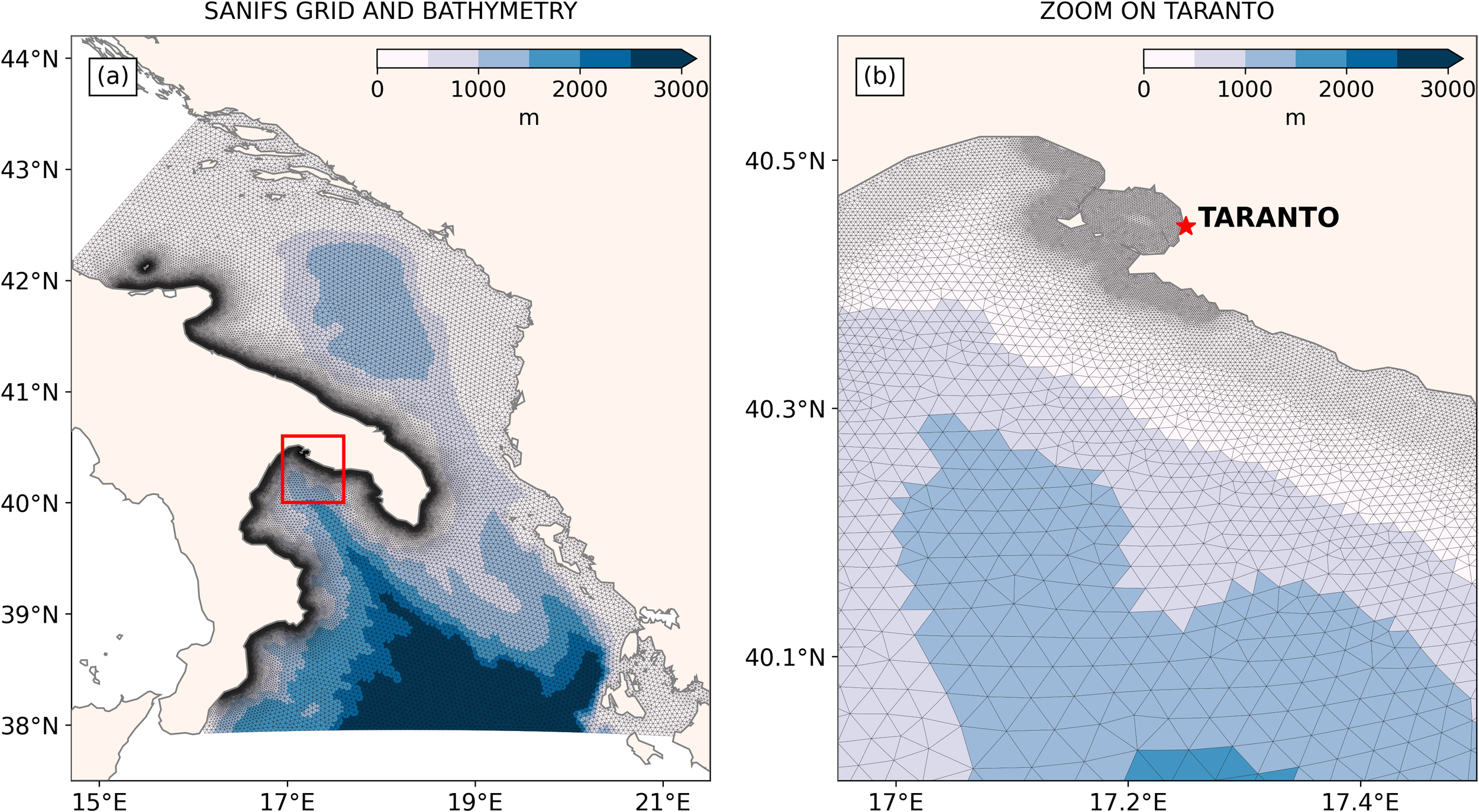
(a) SANIFS numerical domain, grid, and bathymetry. (b) Zoom on the Taranto region.
Table 1
| Model | Domain | Grid | Coastal resolution | Open sea resolution | Levels |
|---|---|---|---|---|---|
| SHYFEM SANIFS implementation Federico et al. (2017) | SANIFS (Figure 1) | Unstructured Arakawa-B triangular mesh 90351 nodes | 50 − 500 m | 3 − 4 km | 92 2 m up to 40 m stepwise up to the bottom max step 200 m |
Summary of the ocean model features.
The original SANIFS system was implemented as a pure downscaling method, re-initialising from the MedFS system every day. In this way, the model also inherits the observational data assimilated into the parent model, and there is less need for a dedicated DA system. However, as the SHYFEM model has matured, it has become feasible and desirable for future applications to run the system in a continuous way without re-initialisation. As the parent model now only provides the lateral open boundary conditions, the assimilation of observations directly into the unstructured grid model is expected to improve the forecast skill.
2.2 OceanVar DA scheme
In this work, SANIFS is interfaced to OceanVar (Dobricic and Pinardi, 2008), which implements a 3DVar data assimilation scheme. Starting from a background state xb, OceanVar aims to find the analysis state xa that corresponds to the x state which minimises the cost function:
Here B is the background covariance matrix, R the observational covariance matrix, y the observation vector and H an observation operator that projects a model state x into observation space.
The background covariance is a positive definite matrix that can be written in the form B = VVT. OceanVar expands V further into a series of distinct operators:
The operator VV models the vertical covariance within a water column by means of empirical orthogonal functions (EOFs) that are derived from the model variability over a longer period. To capture the seasonal changes in the vertical covariance, the EOFs are monthly varying. This part of the covariance is equivalent to a coordinate transformation, providing a pre-conditioned cost function and allowing to reduce the dimensionality of the minimisation problem by truncating the number EOFs. In our case, 25 EOFs are used, computed from a four-year (2017–2020) simulation of SANIFS.
The horizontal covariance operator, VH, describes the covariance between neighbouring water columns at each level. The horizontal covariance is modelled using a Gaussian function, with a correlation length that can be locally varying and is typically proportional to the Rossby radius of deformation. The VH operator is implemented using the first order recursive filter (RF) algorithm of Purser et al. (2003). However, this algorithm is designed for regular grids where neighbouring points are straightforwardly defined in two directions. In order to apply the RF on unstructured triangular meshes, the algorithm has been generalised. This novel approach and algorithm are described in detail in the next section.
Finally, is the dynamic height operator, which balances the steric sea level increment with the temperature and salinity increments in the water column to avoid incoherent analysis states that may cause model instabilities. It additionally provides OceanVar the ability to assimilate sea level observations into a state vector of temperature and salinity without explicitly including the sea level (Storto et al., 2011; Dobricic and Pinardi, 2008). As the dynamic height operator requires calculating the density integral over the water column down to a depth where horizontal velocities are negligible, it is necessary to impose a no-motion level, which we set to 700m. The system is run in offline mode, meaning that the data assimilation step is executed separately from the ocean model forecast. After each assimilation cycle, the updated ocean state is used to initialise the subsequent model run.
2.3 Generalised recursive filter algorithm
Recursive filters are often used in data assimilation to model horizontal covariances, as the covariances are typically Gaussian in shape and the recursive filter is a simple but effective method to impose a Gaussian shape on arbitrary data (Lorenc, 1992; Hayden and Purser, 1995; Purser et al., 2003). The RF is a simple iterative algorithm that requires only a few iterations to approximate the Gaussian function. The algorithm itself is 1-dimensional, but it can be straightforwardly applied in two or more dimensions by alternating dimensions between iterations (Purser et al., 2003). Furthermore, the RF has the ability to locally vary the spread of the Gaussian distribution, which gives it greater flexibility when working with inhomogeneous data. This feature will be indispensable for applying the RF to an unstructured triangular mesh such as for SANIFS.
The mathematical formulation of the RF on a regular grid is relatively straightforward: considering a 1-dimensional field Ai with i =1, 2, 3,…, n, the algorithm consists of a forward pass
followed by a backward pass
where Bi is the field after the first application of the filter, and Ci is the field after one filter pass in each direction. The RF is applied in both directions to ensure zero phase change (Lorenc, 1992).
In Equation 2 and Equation 3, αi is the smoothing factor, defined as:
with Ri the radius of the spread and N the number of iterations. The subscript i denotes the local dependence of the smoothing factor. For a grid with uniform resolution and a constant correlation radius, and the subscripts in Equation 4 can be dropped. The Gaussian spread of the approximate Gaussian is related to the correlation radius and the grid resolution as:
The RF algorithm is applied iteratively N times, and from N ≥ 2 it starts to approximate a Gaussian distribution (Purser et al., 2003). While the RF assumes an infinite domain size, boundary conditions (in open and closed boundaries) can be applied to approximate the infinite line symmetry (Hayden and Purser, 1988; Dobricic and Pinardi, 2008) on a finite domain. The 1D algorithm and its extension to 2D grids is illustrated in Figure 2. The only drawback of the RF algorithm is that with the infinite formulation it is inherently sequential, this makes it difficult to implement in parallelised code.
Figure 2
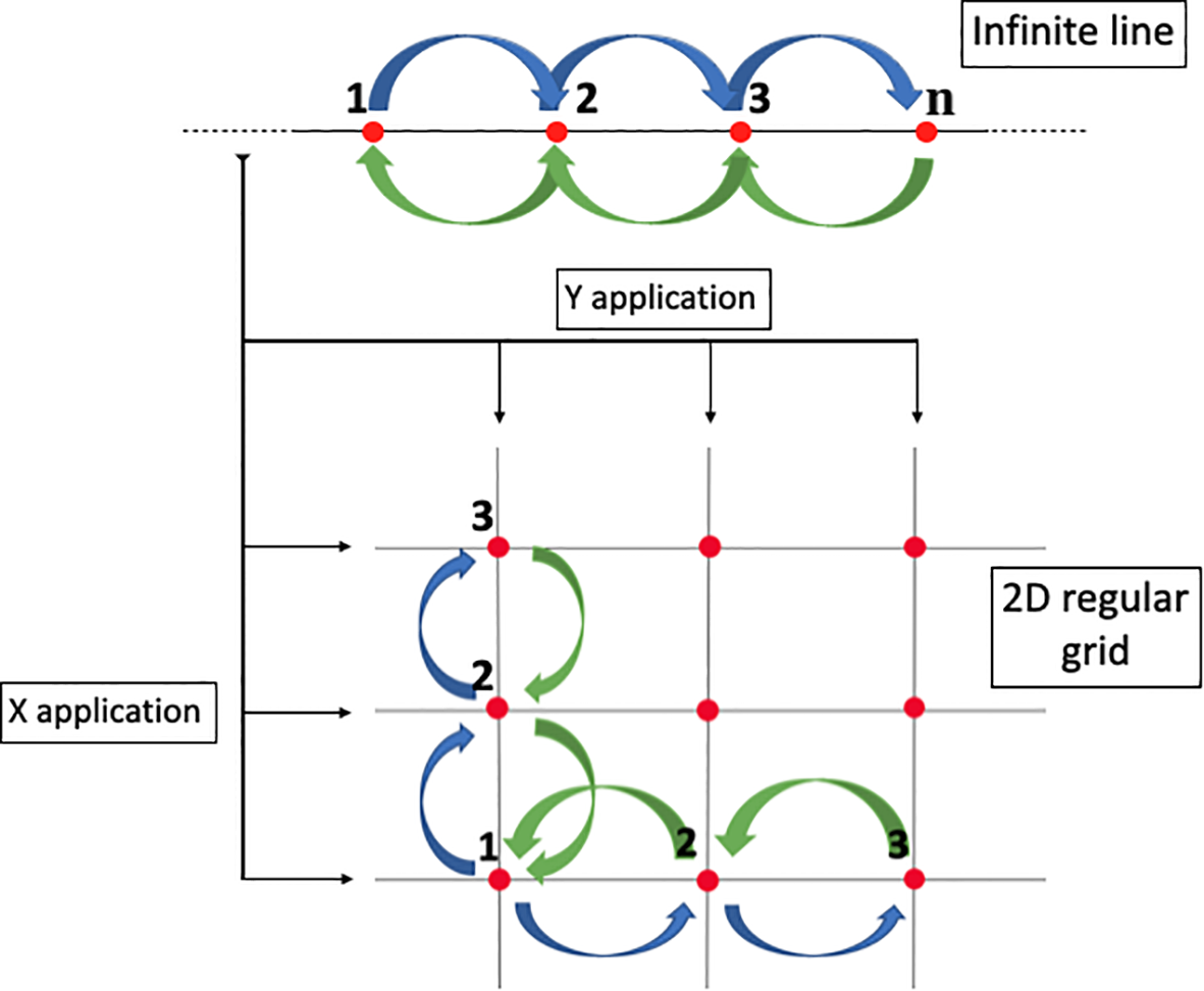
RF infinite line structure and its application on a 2D regular grid. Blue arrows represent the forward pass, and the green arrows are the backward pass.
To apply the RF algorithm to an unstructured mesh, it’s vital to recognise the importance of the node ordering. On a structured mesh, the algorithm processes neighbouring nodes in order (either 1, 2, 3,…, n in the forward pass or n, n − 1, n − 2,… , 1 in the backward pass), which ensures the main requirements for the filter are met:
Each node receives contributions from its neighbour on one side before providing a contribution to its neighbour on the other side;
The forward and backward passes complement each other; the neighbour that provides a contribution in one pass becomes a neighbour that receives a contribution in the opposite pass.
The node ordering problem is therefore really a node connectivity problem and it can be discussed more generally in terms of the mesh edges rather than the nodes themselves. A pass of the recursive filter acting on an edge, directionally propagates information along the edge from one node to the other. In this way the filter can be applied also to triangular unstructured meshes, as long as the above requirements can be met. It turns out that this can be achieved by orienting and ordering the edges appropriately.
First the edges are oriented in the direction of the filter pass, then the edges are sorted by the coordinates of the first node (i.e. the node providing the contribution). If a pass of the filter is imagined as a line of constant longitude or latitude sweeping through the unstructured mesh, these conditions ensure that information is always propagated from nodes at the filter position in the direction that the filter is moving. In this way, the algorithm satisfies the requirements outlined above. The x and y forward and backward passes can be generalised as four passes in the four cardinal directions, orienting and ordering the edges as summarised in Table 2 and in the pseudo-code in the appendix (Algorithm 1).
Table 2
| Filter direction | Edge orientation (primary, secondary) | Edge ordering (first node) |
|---|---|---|
| East (X-FW) | east to west, south to north | increasing longitude, latitude |
| West (X-BW) | west to east, north to south | decreasing longitude, latitude |
| North (Y-FW) | south to north, east to west | increasing latitude, longitude |
| South (Y-BW) | north to south, west to east | decreasing latitude, longitude |
Edge orientation and ordering for the unstructured triangular mesh RF algorithm.
Both orientation and ordering are using a primary and secondary ordering to make sure identical values do not lead to ambiguities.
At this point, the mathematical structure of the RF (Equations 2, 3) can be used, but the running index i is no longer over the nodes but over the edges and all passes of the filter can be described by:
with the ordering and orientation of the edges i as in Table 2 and the subscripts 1 and 2 referring to the first (source) and second (target) nodes of the edge i. The fields A and B are the input and output fields respectively, where B is initialised to 0. The coefficient αi follows from Equation 4, with the resolution corresponding to the length of the edge i. Hereafter, we will refer to the generalised RF algorithm as utRF (unstructured triangular Recursive Filter).
To demonstrate how the utRF reproduces the desired Gaussian symmetry on the SANIFS grid, we show test results using synthetic data with N = 6, which is also the iteration number used in the experiments. Figures 3a, b show results for Ri = R = 8km and Figures 3c, d for Ri = R = 20km. The testing locations have been chosen considering the different grid features on the SANIFS domain. The two points in the Adriatic Sea (1 and 2 in Figure 3a) test the spreading shape in locations with constant resolution, but the grid tessellation is not homogeneous. Furthermore, they are close to each other to demonstrate the spreading shape in the case of intersecting correlation radii (Figure 3c). The point in the middle of the Gulf of Taranto (3) is in a region where grid resolution and triangle tessellation are highly variable. The result on that point shows how the application of the local smoothing factor algorithm avoids extending the Gaussian shape too close to the coast. This aspect is important in real-case applications since it avoids spreading open sea information on the coast. The point in the Ionian open sea (4) is in the middle of an extended region with constant grid resolution and homogeneous triangle tessellation. Finally, a point on the coastline shows how utRF works without boundary conditions in proximity to the closed boundary.
Figure 3
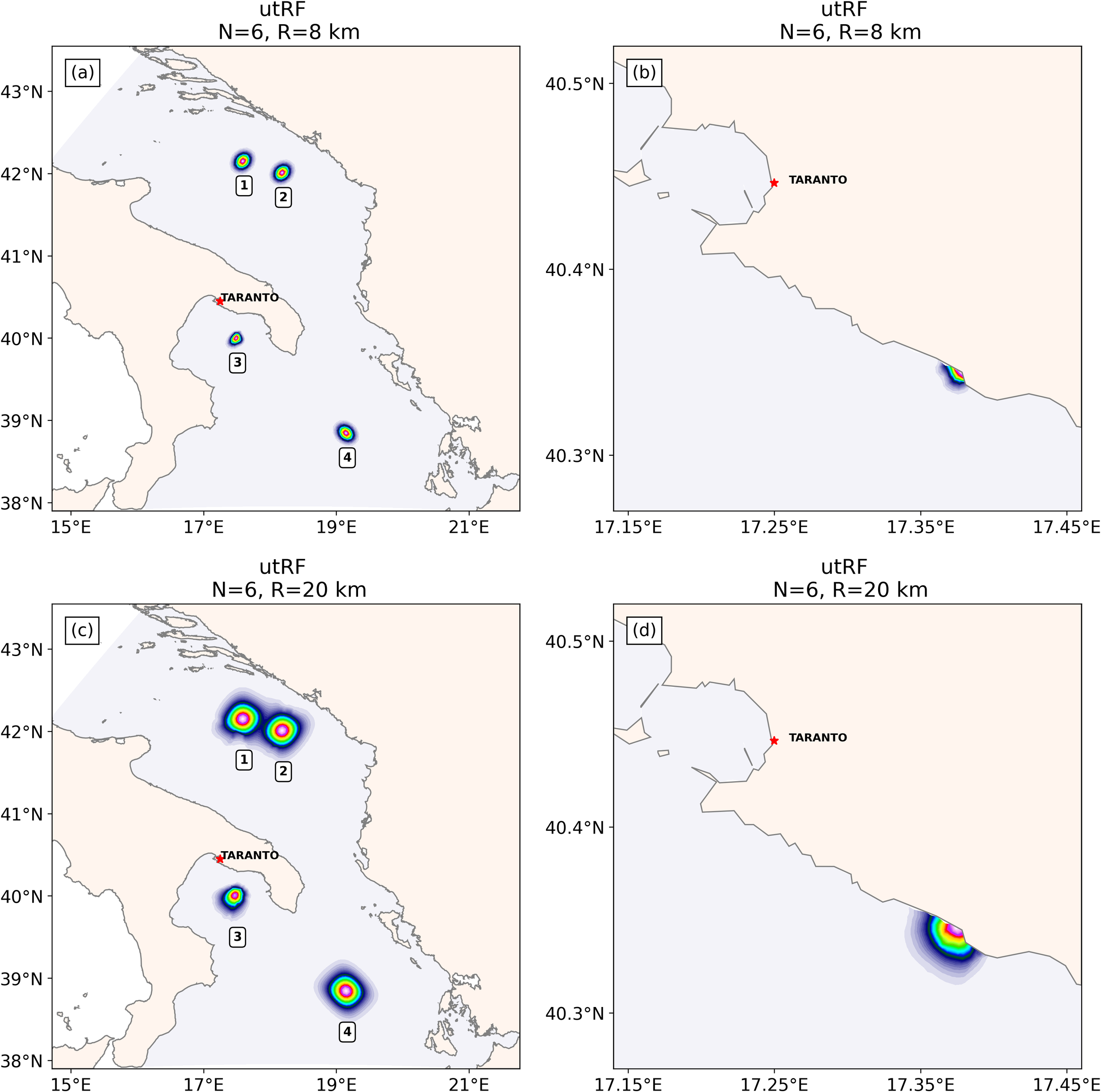
utRF test on synthetic values for different iterations number, N, and a constant correlation radius, R. Points 1–4 in panels (a, c) and the coastal point in panels (b, d) are chosen to cover different regions with different grid features.
From all the cases in Figure 3 we see how the proposed first-order recursive filter for an unstructured triangular grid well approximates the Gaussian spreading using N = 6. We also tested the utRF using different numbers of iterations, and we saw that from N = 2, it starts to approximate a Gaussian spreading as in the case of RF application on a regular grid (results not shown).
2.4 The observational dataset
In OceanVar, we assimilate temperature (T) and salinity (S) from in-situ ARGO profiling floats and sea level anomaly (SLA) from 4 satellite missions: Saral/AltiKa, CryoSat-2, Jason-3 and Sentinel-3A. Both observational products are provided by the Copernicus Marine Service.
Figures 4a, b show, respectively, the assimilated ARGO profiling floats and along-track sea level anomaly distribution over the whole experiment period (2017-2018). The average daily number of ARGO observations assimilated is about 150. 122 days have no ARGO observations. Regarding the SLA, the daily number of assimilated observations is approximately 35. 187 Days have no altimetry observations within the model domain.
Figure 4
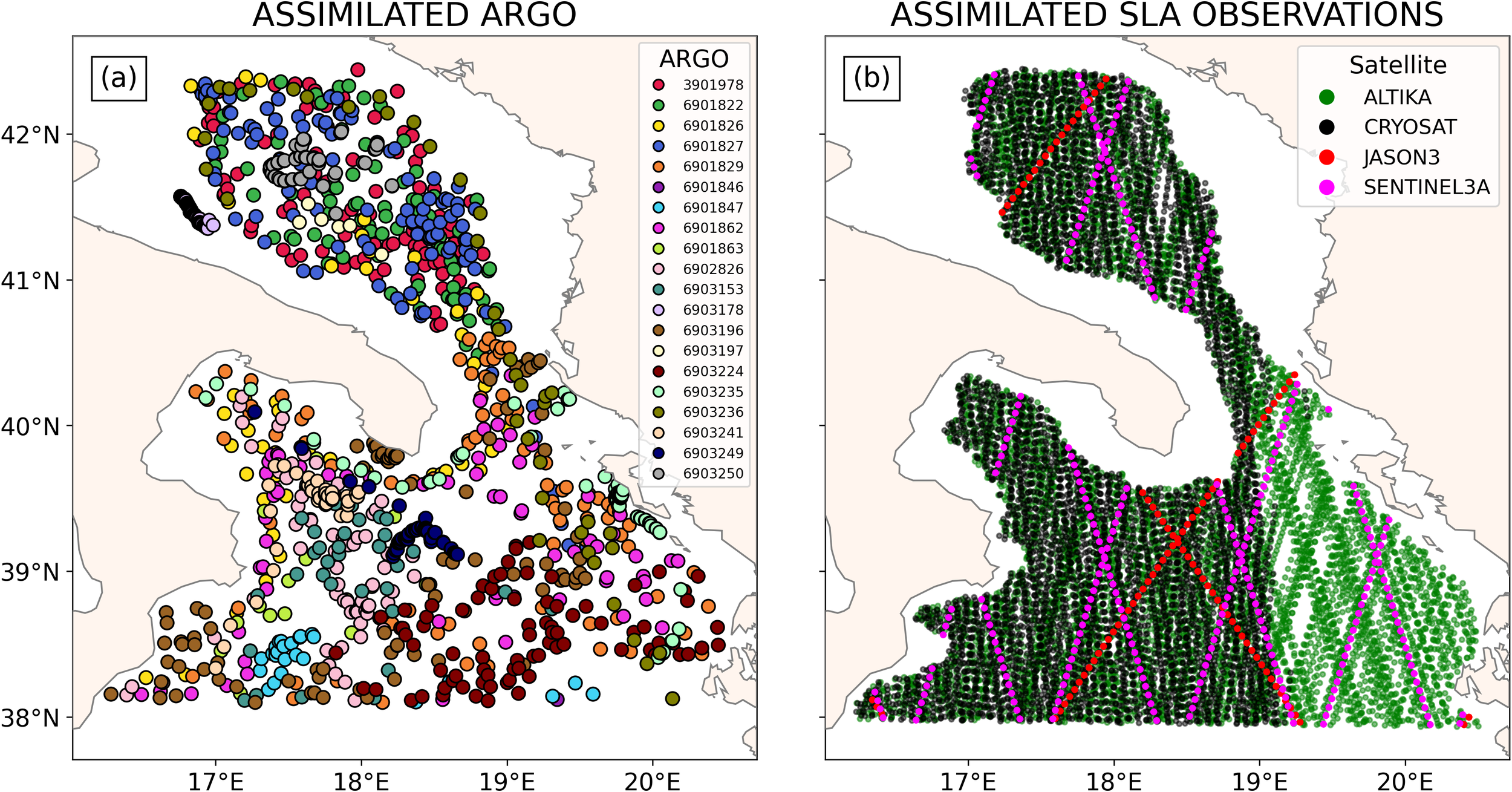
Assimilated ARGO and SLA observations over the period 2017-2018. (a) ARGO profiles (b) along-the-track L3 sea level anomaly observations from altimeter satellites. Each profiler and satellite are shown in different colours.
3 Experiment set-up and results
The data assimilation experiment is performed over the period 2017-2018, with a 10-day spin-up of the SANIFS model. T, S and SLA are assimilated using 25 trivariate EOFs. The experiment uses an assimilation window of 24 hours. The utRF was used with 6 iterations and a correlation radius set to 8km. The results are compared to a control experiment without DA.
Since the assimilation of SLA has a net positive impact on SLA and a negligible impact on the skills for T and S, the results presented here will focus on the experiment that includes all three variables. This choice enables the integrated discussion of the skill scores for all variables that are commonly assimilated in ocean models.
The SANIFS modelling system with DA alternates between running SHYFEM and OceanVar in steps of 24 hours. These form the assimilation windows in which the output of the SHYFEM model is compared to the available observations within the window. OceanVar calculates the minimum of the cost function using the model background read from the output fields and calculates the analysis increments. The increments are applied to the SHYFEM restart files at the start of the next 24-hour cycle. Figure 5 shows an example of a typical set of analysis increments on the unstructured grid, with the horizontal spread (R = 8km) modelled using the novel utRF algorithm. Similarly to the test performed on a synthetic dataset in Figure 3, the utRF implemented in OceanVar shows a good approximation of the Gaussian horizontal covariance. Moreover, the figure shows how the triradiate dynamic height operator produces increments in S and T fields from SLA observations (Figures 5a, b) and vice versa S and T observations produce increments in the SLA field (Figure 5c). The presence of SLA observations can be inferred from the spatial arrangement of the corresponding increments, which appear as regularly spaced and aligned features, reflecting the along-track structure of altimetric satellite measurements.
Figure 5
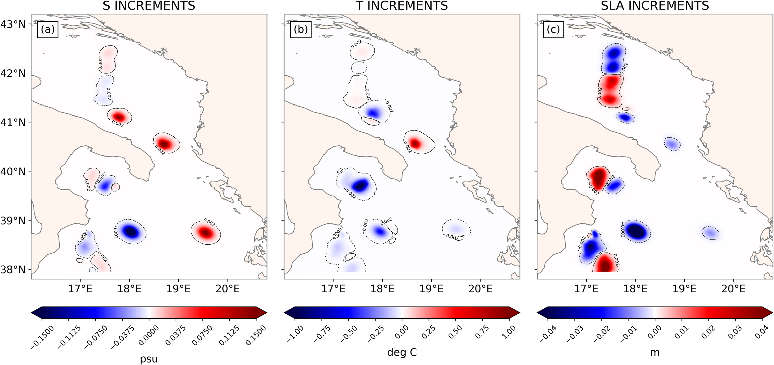
Example on 2017–09–05 of increments spreading shape for the two sources of observation assimilated (ARGO and altimetry satellites). The figure shows how the utRF approximates the Gaussian shape and how the dynamic height operator produces increments in S and T fields from SLA observations, (a, b), and vice versa S and T observations produce increments in the SLA field (c). The utRF parameters are: N = 6, R = 8km.
Following the methodology of Dobricic and Pinardi (2008), the analysis is evaluated using a quasi-independent set of measurements. In practice, this means that the same ARGO and satellite data used in the assimilation cycle were first applied for validation before being assimilated into the analysis. The evaluation relies on the misfits (observation minus background), which are computed prior to the assimilation of the corresponding observations. These misfits are expected to decrease compared to the control run without data assimilation. In addition, the residuals (observation minus analysis) are examined to quantify the magnitude of the corrections introduced into the model.
Figure 6 shows the daily mean absolute value of the misfits versus the daily mean absolute value of the residuals (observations minus analysis) for S, T and SLA. The straight line indicates a slope of 1. For S (Figures 6a–d) and T (Figures 6f-i), the results are divided in four different water column layers to investigate the improvement of various SANIFS system features:
Figure 6
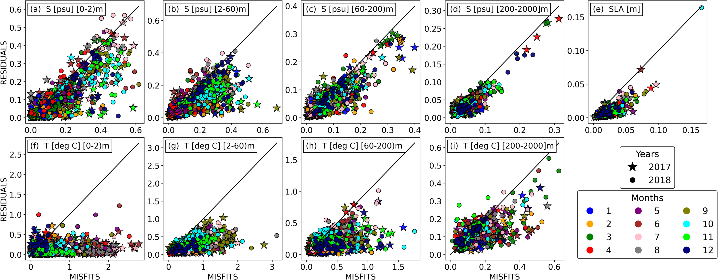
S, T and SLA mean absolute value of misfits and residuals. In (a–d) and (f–i) we show different water column layers for S and T. (e) refers to SLA. Different colours refer to different months. Stars for 2017 and circles for 2018.
(0,2]m - This layer is intended to investigate near-surface T and S features. The near-surface layer is one of the most difficult to be represented in oceanographic models. It is directly affected by atmospheric forces such as wind, solar radiation, rain, and rivers from the land.
(2,60]m - This layer is intended to investigate T and S features in the mixing layer. Like the near-surface layer, the mixing layer presents challenges in oceanographic modelling. The thermocline seasonal variability and some inputs propagating from the surface through turbulence and heat exchange complicate modelling in this layer.
(60,200]m - This layer is intended to investigate T and S features in the region of the water column that approaches the deep water layer. Here, the thermocline seasonal variability can still affect the modelling skills.
(200,2000]m - This layer is intended to investigate T and S features in the region of the water column in which there are no particular challenges and the errors are expected to be smaller.
The assumption that the model error is smaller in deep ocean layers is supported by the recent study of Benincasa et al. (2024), who showed that the atmospherically forced response in the Mediterranean Sea decreases rapidly with depth, while internal variability dominates mainly in the upper ocean. Below a few hundred meters, the system is comparatively more stable and less sensitive to external perturbations.
Results confirm this interpretation. For both T and S, the daily mean absolute values of the misfits and residuals decrease from the surface to the deeper layers. All panels show that most of the points are below the slope-1 line for both variables, meaning that our assimilation is improving the local background state. In particular, for T, it can be observed how we are introducing a consistent correction in the first three layers (Figures 6f-h). All the points are well below the diagonal line. For the layer (0,2]m (Figure 6f), we see T residuals well below 2°C of the corresponding misfit. In the two lower layers, we are introducing an improvement of about 1°C. In the layer (200-2000] m (Figures 6d-i), we see how the model well reproduces both S and T. Finally, Figure 6e refers to SLA. Here, considering that the majority of the points are below the diagonal line, we can conclude that SLA improves in a consistent way by assimilating altimetry observations.
After the evaluation of the individual corrections, the performance of the system as a whole is evaluated using only the quasi-independent measurements (i.e. misfits). The 1-day forecast skill of the system is evaluated by means of the skill score (Murphy, 1988), which is defined as:
The skill score depends on the ratio of the mean square error (MSE) of the experiment with DA (denoted exp) and the control experiment without DA (denoted ref). The skill score is constructed in such a way that it ranges from a value of 1 for an experiment that agrees perfectly with the observations to 0 for an experiment that shows no improvement over the reference model. If the experiment performs worse than the reference, the skill score can assume any negative value. The skill score is visualised in profiles for S and T (Figure 7) and maps for all variables (Figure 8) for the DA experiment in comparison with the control experiment, which does not include DA.
Figure 7
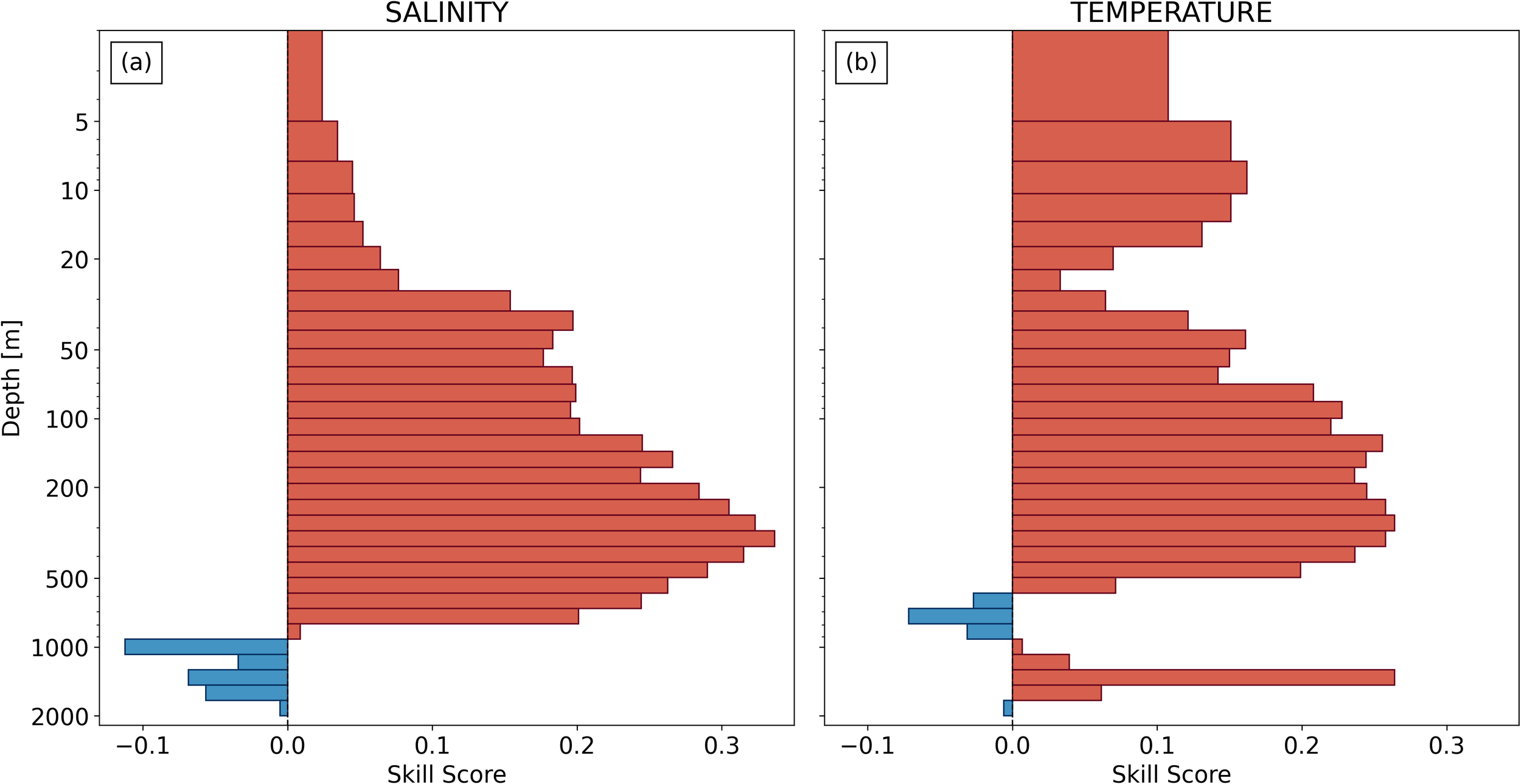
Skill scores of the data assimilation experiment compared to the control experiment without data assimilation for (a) salinity and (b) temperature as a function of depth. Positive (red) values indicate an improved model skill with data assimilation.
Figure 8
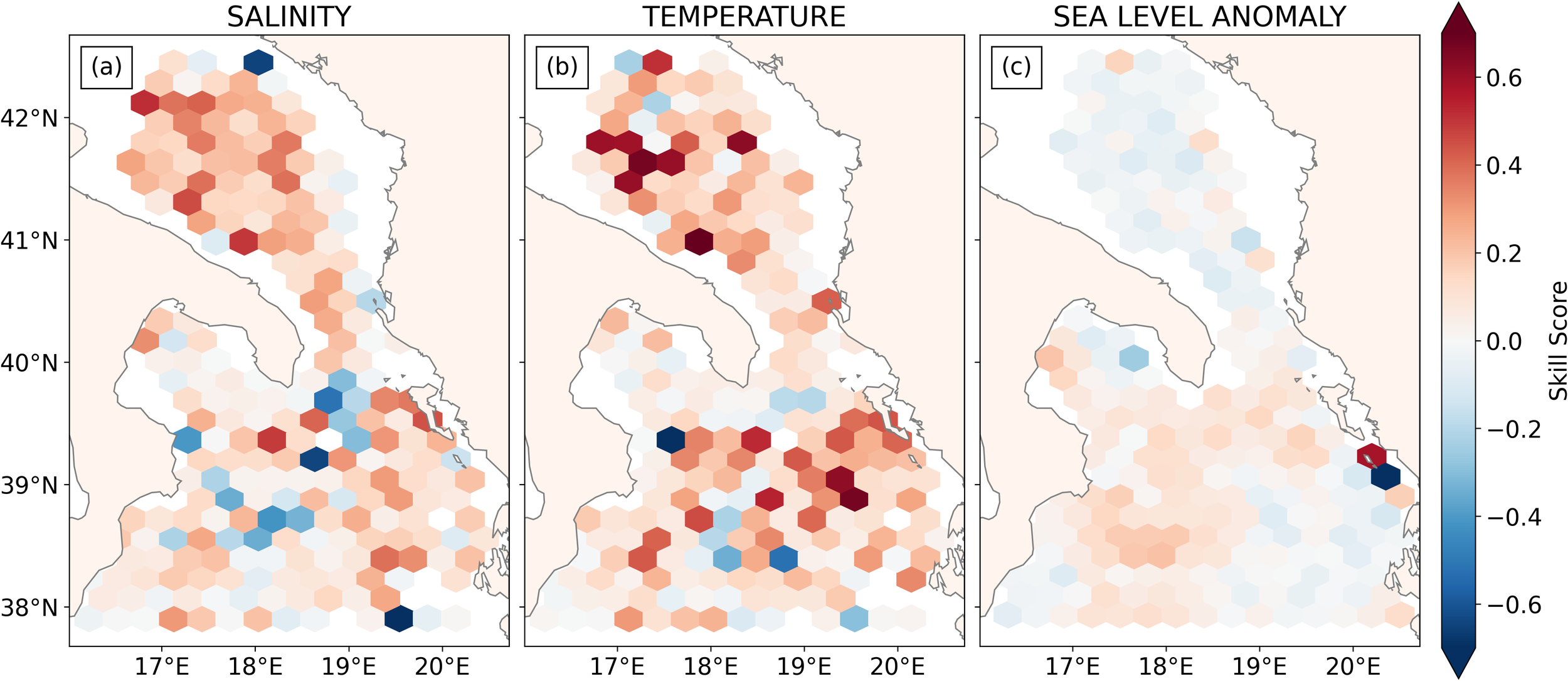
Skill scores of the data assimilation experiment compared to the control experiment without data assimilation for (a) salinity, (b) temperature, and (c) SLA projected on the model domain. Positive (red) values indicate an improved model skill with data assimilation.
The salinity skill in Figure 7a shows a consistent improvement from the surface down to a depth of around 900m. Below the thermocline the improvement in MSE is above 20%, with a maximum of almost 35% around 300m. Below 1000m some negative skills are found. This is most likely related to the fact that only about 1 in 6 ARGO profiles extend below 1000m. Increments originating from shallow profiles that are applied below 1000m depend very strongly on the correct modelling of the covariance matrix and are probably less accurate.
The temperature skill in Figure 7b exhibits a very similar improvement down to approximately 600m. In the mixed layer the MSE improves by more than 10%, while the improvement reduces somewhat around the average depth of the thermocline. The skill score reaches a maximum of over 0.2 for the layers between 100m and 500m. Below 600m some layers show a small degradation in MSE with a maximum of around 5%.
Figure 8 provides spatial maps illustrating how the improvements introduced by data assimilation are distributed across the SANIFS domain. For both S and T, positive skill scores are observed at the majority of the observation locations. Conversely, sea level anomaly (SLA) exhibits positive values predominantly in the northern Ionian region, while negative values are evident in the southern Adriatic. This discrepancy may be attributed to diurnal variations of sea level and/or the incomplete description of tides in the model.
The impact of data assimilation on the circulation is evaluated by comparing the barotropic velocities between the assimilation and control experiments. Figure 9 shows the annual mean fields for 2018. The difference in magnitude is displayed in Figure 9a, and the circulation in the experiment with data assimilation is shown in Figure 9b. The results indicate a 5–10% intensification of both the Southern Adriatic Gyre and the Western Adriatic Current. While additional differences are present at shorter timescales in other parts of the basin, these largely cancel out in the long-term averages. Importantly, the assimilation does not alter the direction or structure of the major gyres and currents, resulting in no significant impact on the overall circulation pattern.
Figure 9
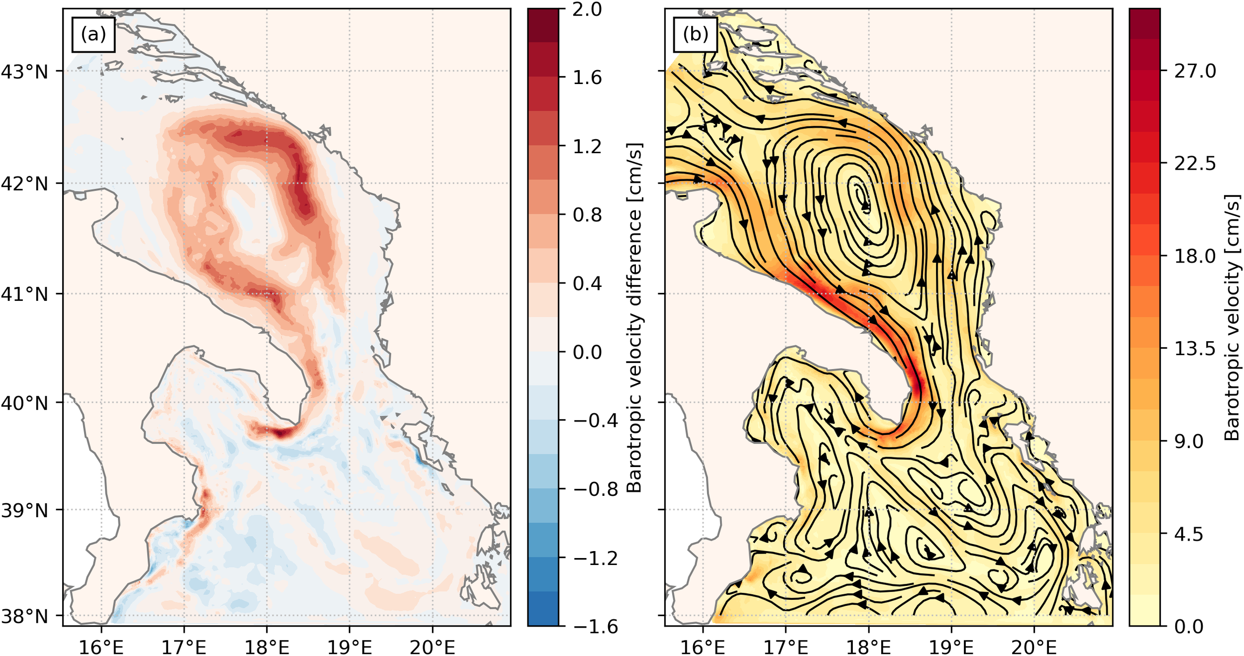
The effect of the assimilation on the mean barotropic velocity in the year 2018. Showing (a) the difference in magnitude between the assimilation and the control run, and (b) the velocity field and its absolute magnitude.
As a future improvement, we propose implementing the First Guess at Appropriate Time (FGAT) approach. FGAT would allow for comparing the SLA observations to the instantaneous model SLA at the correct time, rather than to a mean value. This enables a more correct treatment of the tidal signal, potentially addressing the observed limitations and further enhancing the performance of the system.
4 Conclusions
The OceanVar 3DVar data assimilation scheme has been successfully implemented in the SANIFS modelling system based on the SHYFEM-MPI unstructured grid model. The first-order recursive filter algorithm of Purser et al. (2003) for regular grids has been generalised to unstructured meshes and implemented in the OceanVar software. The new system has been used to assimilate ARGO in-situ profiles and SLA from satellite during the period 2017-2018. The results are compared to a control run without DA.
The results for assimilating in-situ profiles are very promising, showing a consistent improvement of the model skill over the entire domain and across nearly all depth levels. The improvement is especially notable in the 100-500m depth range, where data assimilation reduces the mean absolute error of S and T by 25–30%.
The assimilation of SLA has a much smaller impact but nevertheless shows an overall improvement of the MAE of 3% and, especially in the southern part of the domain, improvements that locally reach up to 20%. The reason for the smaller impact of SLA is believed to be primarily technical and will be the subject of future work. At present, for example, the model background estimates use average values, while in the presence of tides, instantaneous values should be preferred. Moreover, there is no mean dynamic topography calculated from the SANIFS model yet, and the SLA experiment used an interpolated low-resolution regular-grid MDT. This may be an additional source of errors.
Overall, the new implementation has been shown to work correctly and to have a positive impact on the model performance. The experiments show promise for a future operational coastal model with data assimilation using this new methodology.
Statements
Data availability statement
The raw data supporting the conclusions of this article will be made available by the authors, without undue reservation.
Author contributions
MS: Data curation, Methodology, Investigation, Software, Formal analysis, Validation, Visualization, Writing – original draft, Writing – review & editing. EJ: Conceptualization, Methodology, Software, Formal analysis, Validation, Visualization, Supervision, Writing – original draft, Writing – review & editing. AA: Conceptualization, Methodology, Software, Supervision, Writing – original draft, Writing – review & editing. IF: Funding acquisition, Resources, Conceptualization, Supervision, Project administration, Writing – original draft, Writing – review & editing. GC: Funding acquisition, Conceptualization, Supervision, Project administration, Writing – original draft, Writing – review & editing.
Funding
The author(s) declare financial support was received for the research and/or publication of this article. Part of this study was funded by the FOCCUS project (Grant Agreement No. 101133911, European Union). This study was carried out within the Space It Up project funded by the Italian Space Agency, ASI, and the Ministry of University and Research, MUR, under contract n. 2024-5-E.0 - CUP n. I53D24000060005. MS is supported by the European Union’s Horizon Europe research and innovation program under the Marie Sklodowska-Curie COFUND Postdoctoral Programme, co-funded under the grant agreement No.101081355 - SMASH and by the Republic of Slovenia and the European Union from the European Regional Development Fund.
Conflict of interest
The authors declare that the research was conducted in the absence of any commercial or financial relationships that could be construed as a potential conflict of interest.
The handling editor SB declared a past co-authorship with the authors EJ, IF and GC.
Generative AI statement
The author(s) declare that no Generative AI was used in the creation of this manuscript.
Any alternative text (alt text) provided alongside figures in this article has been generated by Frontiers with the support of artificial intelligence and reasonable efforts have been made to ensure accuracy, including review by the authors wherever possible. If you identify any issues, please contact us.
Correction note
A correction has been made to this article. Details can be found at: 10.3389/fmars.2026.1792768.
Publisher’s note
All claims expressed in this article are solely those of the authors and do not necessarily represent those of their affiliated organizations, or those of the publisher, the editors and the reviewers. Any product that may be evaluated in this article, or claim that may be made by its manufacturer, is not guaranteed or endorsed by the publisher.
Author disclaimer
Co-funded by the European Union. Views and opinions expressed are, however, those of the author(s) only and do not necessarily reflect those of the European Union or European Research Executive Agency. Neither the European Union nor the granting authority can be held responsible for them.
Footnotes
References
1
AndersonJ.HoarT.RaederK.LiuH.CollinsN.TornR.et al. (2009). The Data Assimilation Research Testbed: A community facility. Bull. Am. Meteorological Soc.90, 1283–1296. doi: 10.1175/2009BAMS2618.1
2
AydoğduA.HoarT. J.VukicevicT.AndersonJ. L.PinardiN.KarspeckA.et al. (2018). OSSE for a sustainable marine observing network in the Sea of Marmara. Nonlinear Processes Geophysics25, 537–551. doi: 10.5194/npg-25-537-2018
3
BajoM. (2020). Improving storm surge forecast in Venice with a unidimensional Kalman filter. Estuarine Coast. Shelf Sci.239, 106773. doi: 10.1016/j.ecss.2020.106773
4
BellafioreD.UmgiesserG. (2010). Hydrodynamic coastal processes in the north Adriatic investigated with a 3D finite element model. Ocean Dynamics60, 255–273. doi: 10.1007/s10236-009-0254-x
5
BenincasaR.LiguoriG.PinardiN.Von StorchH. (2024). Internal and forced ocean variability in the Mediterranean Sea. Ocean Sci.20, 1003–1012. doi: 10.5194/os-20-1003-2024
6
BlumbergA. F.MellorG. L. (1987). A description of a three-dimensional coastal ocean circulation model. Three-dimensional Coast. ocean Models4, 1–16. doi: 10.1029/CO004
7
BurchardH.PetersenO. (1999). Models of turbulence in the marine environment—a comparative study of two-equation turbulence models. J. Mar. Syst.21, 29–53. doi: 10.1016/S0924-7963(99)00004-4
8
ChenC.BeardsleyR. C.CowlesG.QiJ.LaiZ.GaoG.et al. (2006). An unstructured grid, finite-volume coastal ocean model: FVCOM user manual Vol. 6 (New Bedford, MA: SMAST/UMASSD), 78.
9
ChenC.Malanotte-RizzoliP.WeiJ.BeardsleyR. C.LaiZ.XueP.et al. (2009). Application and comparison of Kalman filters for coastal ocean problems: an experiment with FVCOM. J. Geophysical Research: Oceans114, C05011. doi: 10.1029/2007JC004548
10
CoppiniG.ClementiE.CossariniG.SalonS.KorresG.RavdasM.et al. (2023). The Mediterranean Forecasting System–part 1: Evolution and performance. Ocean Sci.19, 1483–1516. doi: 10.5194/os-19-1483-2023
11
CuccoA.UmgiesserG. (2006). Modeling the Venice Lagoon residence time. Ecol. Model.193, 34–51. doi: 10.1016/j.ecolmodel.2005.07.043
12
DobricicS.PinardiN. (2008). An oceanographic three-dimensional variational data assimilation scheme. Ocean Model.22, 89–105. doi: 10.1016/j.ocemod.2008.01.004
13
EgbertG. D.ErofeevaS. Y. (2002). Efficient inverse modeling of barotropic ocean tides. J. Atmospheric Oceanic Technol.19, 183–204. doi: 10.1175/1520-0426(2002)019<0183:EIMOBO>2.0.CO;2
14
EvensenG. (1994). Sequential data assimilation with a nonlinear quasi-geostrophic model using Monte Carlo methods to forecast error statistics. J. Geophysical Research: Oceans99, 10143–10162. doi: 10.1029/94JC00572
15
EvensenG. (2003). The ensemble Kalman filter: Theoretical formulation and practical implementation. Ocean dynamics53, 343–367. doi: 10.1007/s10236-003-0036-9
16
EvensenG. (2009). The ensemble Kalman filter for combined state and parameter estimation. IEEE Control Syst. Magazine29, 83–104. doi: 10.1109/MCS.2009.932223
17
FedericoI.PinardiN.CoppiniG.OddoP.LecciR.MossaM. (2017). Coastal ocean forecasting with an unstructured grid model in the southern Adriatic and northern Ionian seas. Natural Hazards Earth System Sci.17, 45–59. doi: 10.5194/nhess-17-45-2017
18
FerrarinC.BajoM.UmgiesserG. (2021). Model-driven optimization of coastal sea observatories through data assimilation in a finite element hydrodynamic model (SHYFEM v. 7_5_65). Geosci. Model Dev.14, 645–659. doi: 10.5194/gmd-14-645-2021
19
FerrarinC.RolandA.BajoM.UmgiesserG.CuccoA.DavolioS.et al. (2013). Tide surge-wave modelling and forecasting in the Mediterranean Sea with focus on the Italian coast. Ocean Model.61, 38–48. doi: 10.1016/j.ocemod.2012.10.003
20
FofonoffN. (1985). Physical properties of seawater: A new salinity scale and equation of state for seawater. J. Geophysical Research: Oceans90, 3332–3342. doi: 10.1029/JC090iC02p03332
21
GruberN. (2011). Warming up, turning sour, losing breath: ocean biogeochemistry under global change. Philos. Trans. R. Soc. A: Mathematical Phys. Eng. Sci.369, 1980–1996. doi: 10.1098/rsta.2011.0003
22
HaydenC. M.PurserR. J. (1988). Three-dimensional recursive filter objective analysis of meteorological fields. In Eighth Conference on Numerical Weather Prediction. Baltimore, American Meteorological Society, 185–190.
23
HaydenC. M.PurserR. J. (1995). Recursive filter objective analysis of meteorological fields: Applications to NESDIS operational processing. J. Appl. Meteorology Climatology34, 3–15. doi: 10.1175/1520-0450-34.1.3
24
HellermanS.RosensteinM. (1983). Normal monthly wind stress over the world ocean with error estimates. J. Phys. Oceanography13, 1093–1104. doi: 10.1175/1520-0485(1983)013<1093:NMWSOT>2.0.CO;2
25
LimaL.CilibertiS. A.AydogduA.EscudierR.MasinaS.AzevedoD.et al. (2021). “ The new Black Sea reanalysis system within CMEMS,” In EGU General Assembly Conference Abstracts. EGU21–E9599.
26
LorencA. (1992). Iterative analysis using covariance functions and filters. Q. J. R. Meteorological Soc.118, 569–591. doi: 10.1002/qj.49711850509
27
MaicuF.AlessandriJ.PinardiN.VerriG.UmgiesserG.LovoS.et al. (2021). Downscaling with an unstructured coastal-ocean model to the Goro Lagoon and the Po river delta branches. Front. Mar. Sci.8, 647781. doi: 10.3389/fmars.2021.647781
28
Masson-DelmotteV.ZhaiP.PörtnerH.-O.RobertsD.SkeaJ.ShuklaP. R.et al. (2018). Global warming of 1.5°C: An IPCC special report on impacts of global warming of 1.5°C above pre-industrial levels and related global greenhouse gas emission pathways, in the context of strengthening the global response to the threat of climate change, sustainable development, and efforts to eradicate poverty. Sustainable Development, and Efforts to Eradicate Poverty32.
29
MicalettoG.BarlettaI.MocaveroS.FedericoI.EpicocoI.VerriG.et al. (2021). Parallel implementation of the SHYFEM model (SANIFS_v1) ( Zenodo). doi: 10.5281/zenodo.5596734
30
MurphyA. H. (1988). Skill scores based on the mean square error and their relationships to the correlation coefficient. Monthly weather Rev.116, 2417–2424. doi: 10.1175/1520-0493(1988)116<2417:SSBOTM>2.0.CO;2
31
NergerL.TangQ.MuL. (2019). Efficient ensemble data assimilation for coupled models with the Parallel Data Assimilation Framework: Example of AWI-CM. Geoscientific Model. Dev. Discussions2019, 1–23. doi: 10.5194/gmd-2019-167
32
PaulsonC. A.SimpsonJ. J. (1977). Irradiance measurements in the upper ocean. J. Phys. Oceanography7, 952–956. doi: 10.1175/1520-0485(1977)007<0952:IMITUO>2.0.CO;2
33
PettenuzzoD.LargeW.PinardiN. (2010). On the corrections of ERA-40 surface flux products consistent with the Mediterranean heat and water budgets and the connection between basin surface total heat flux and NAO. J. Geophysical Research: Oceans115, C06022. doi: 10.1029/2009JC005631
34
PurserR. J.WuW.-S.ParrishD. F.RobertsN. M. (2003). Numerical aspects of the application of recursive filters to variational statistical analysis. Part I: Spatially homogeneous and isotropic Gaussian covariances. Monthly Weather Rev.131, 1524–1535. doi: 10.1175//1520-0493(2003)131<1524:NAOTAO>2.0.CO;2
35
SmagorinskyJ. (1963). General circulation experiments with the primitive equations: I. the basic experiment. Monthly Weather Rev.91, 99–164. doi: 10.1175/1520-0493(1963)091<0099:GCEWTP>2.3.CO;2
36
StortoA.DobricicS.MasinaS.Di PietroP. (2011). Assimilating along-track altimetric observations through local hydrostatic adjustment in a global ocean variational assimilation system. Monthly Weather Rev.139, 738–754. doi: 10.1175/2010MWR3350.1
37
StortoA.MasinaS.NavarraA. (2016). Evaluation of the CMCC Eddy-Permitting Global Ocean Physical Reanalysis System (C-GLORS 1982–2012) and its assimilation components. Q. J. R. Meteorological Soc.142, 738–758. doi: 10.1002/qj.2673
38
UmgiesserG.CanuD. M.CuccoA.SolidoroC. (2004). A finite element model for the Venice Lagoon. Development, set up, calibration and validation. J. Mar. Syst.51, 123–145. doi: 10.1016/j.jmarsys.2004.05.009
39
WangQ.DanilovS.SidorenkoD.TimmermannR.WekerleC.WangX.et al. (2014). The Finite Element Sea Ice-Ocean Model (FESOM) v. 1.4: formulation of an ocean general circulation model. Geoscientific Model. Dev.7, 663–693. doi: 10.5194/gmd-7-663-2014
40
ZhuZ.-N.ZhuX.-H.GuoX.FanX.ZhangC. (2017). Assimilation of coastal acoustic tomography data using an unstructured triangular grid ocean model for water with complex coastlines and islands. J. Geophysical Research: Oceans122, 7013–7030. doi: 10.1002/2017JC012715
Appendix
Algorithm 1 implements the directional iterative recursive filter algorithm for triangular unstructured grids, referred to as utRF in the text and discussed in section 2.3.
Algorithm 1
Data: Nodes with longitude/latitude; edges referencing two nodes; input field input(·)
Result:output(·) after iterative directional utRF application as Equation 5
1 struct node
2            float lon, lat
3        struct edges
4            float alpha; node nodes[2]
56 foreachedge ∈ edgesdo7            # Calculate α using Equation 4 and use the node distance as δ
              edge.alpha ← alpha_from_distance (edge.node[0], edge.node[1])
8 foriteration ← 1toNdo9        foreachdirection ∈ {east, west, north, south}do10output•) ← 0
11             ifdirection == eastthen12                   foreachedge ∈ edgesdo13                          sort edge.nodes by increasing node[0].lon (then node[0].lat)
14            else ifdirection == westthen15                    foreachedge ∈ edgesdo16                      sort edge.nodes by decreasing node[1].lon (then node[1].lat)
17            else ifdirection == norththen18                    foreachedge ∈ edgesdo19                       sort edge.nodes by increasing node[0].lat (then node[0].lon)
20            else ifdirection == souththen21                    foreach edge ∈ edges do22                   sort edge.nodes by decreasing node[1].lat (then node[1].lon)
23            foreachedge ∈ edgesdo24output(edge.nodes[1]) ← edge.alpha • output (edge.nodes[0]) + (1 − edge.alpha) •
                         input(edge.nodes[1])
25input(•) ← output (•)
Summary
Keywords
coastal ocean, variational data assimilation, unstructured grid ocean modelling, 3DVAR, unstructured grid first order recursive filter algorithm, recursive filter
Citation
Stefanelli M, Jansen E, Aydoğdu A, Federico I and Coppini G (2025) Data assimilation for advanced cross-scale unstructured grid ocean modelling. Front. Mar. Sci. 12:1656879. doi: 10.3389/fmars.2025.1656879
Received
30 June 2025
Accepted
30 September 2025
Published
17 November 2025
Corrected
28 January 2026
Volume
12 - 2025
Edited by
Simone Bonamano, University of Tuscia, Italy
Reviewed by
Yuntao Wang, Ministry of Natural Resources, China
Fernando Barreto, OceanPact Servicos Maritimos, Brazil
Updates
Copyright
© 2025 Stefanelli, Jansen, Aydoğdu, Federico and Coppini.
This is an open-access article distributed under the terms of the Creative Commons Attribution License (CC BY). The use, distribution or reproduction in other forums is permitted, provided the original author(s) and the copyright owner(s) are credited and that the original publication in this journal is cited, in accordance with accepted academic practice. No use, distribution or reproduction is permitted which does not comply with these terms.
*Correspondence: Marco Stefanelli, marco.stefanelli@cmcc.it; marco.stefanelli@fmf.uni-lj.si
Disclaimer
All claims expressed in this article are solely those of the authors and do not necessarily represent those of their affiliated organizations, or those of the publisher, the editors and the reviewers. Any product that may be evaluated in this article or claim that may be made by its manufacturer is not guaranteed or endorsed by the publisher.